Assessing competitive balance in the English Premier League for over forty seasons using a stochastic block model

Abstract

Competitive balance is the subject of much interest in the sports analytics literature and beyond. In this paper, we develop a statistical network model based on an extension of the stochastic block model to assess the balance between teams in a league. Here we represent the outcome of all matches in a football season as a dense network with nodes identified by teams and categorical edges representing the outcome of each game as a win, draw or a loss. The main focus and motivation for this paper is to provide a statistical framework to assess the issue of competitive balance in the context of the English First Division / Premier League over more than $40$ seasons. The Premier League is arguably one of the most popular leagues in the world, in terms of its global reach and the revenue which it generates. Therefore it is of wide interest to assess its competitiveness. Our analysis provides evidence suggesting a structural change around the early 2000’s from a reasonably balanced league to a two-tier league.

Keywords Bayesian statistics  $\cdot$ sports analytics  $\cdot$ Markov Chain Monte Carlo  $\cdot$ stochastic block model  $\cdot$ competitive balance

1 Introduction

Uncertainty in the outcome in sporting events would, on the face of it, appear to be an essential ingredient of attractive team sports (Szymanski, 2001). The study of competitive balance is one which has interested researchers for some time, particularly in fields as diverse as economics to sports science. For example, there is much interest to investigate relationships between the competitiveness of a sporting league and the distribution of revenue within the league. For example, Brandes and Franck (2007) study the effect which competitiveness of the Bundesliga in Germany has on attendance while Manasis et al. (2022) study the effect of competitiveness for several European leagues; see also (Penn and Berridge, 2019) and (Plumley et al., 2018) who present a perspective in the context of the English Premier League. More generally, competitive balance is of vital interest and used as an argument by sports governing bodies to ensure that, for example, revenue streams are allocated proportionately. In fact, in the context of soccer, that was partly the reason for introducing the UEFA Financial Fair Play Regulations (FFP) to limit excessive spending and investments by club owners together with the intention to ensure that clubs budgets are regulated, reducing debts from season to season and creating profit. The new regulations were agreed in 2009 and put in practice three years later.

In the literature of sports analytics, several authors have proposed statistical measures of competitive balance. Most of these indices are based on intuition about the notion of competitiveness. These are typically descriptive statistics based on summarising the spread of points or wins achieved by each team at the end of the league, see (Evans, 2014) and references therein. For example, the Herfindahl–Hirschman index of competitive balance is adapted from the Herfindahl-Hirschman index which is used to measure the spread of market share by firms in a given industry. Other definitions are based on the idea of entropy among many others. We refer the reader to (Manasis et al., 2013) for a statistical perspective on this topic; see also (Evans, 2014) for a comprehensive review of this literature. A thorough search of the related methodology reveals very few publications with competitive balance indexes which are based on solid statistical models or techniques. Some exceptions include the approach of Koning (2000) based on multinomial probit type of model with response the game outcome (win, draw, loss), the index introduced by Haan et al. (2008) based on a regression model for the goal difference, and the autoregressive win percentage by Vrooman (1995) which is based on an auto-regressive model. Further, model-based approaches are the variance decomposition measure (Eckard, 1998) and CBR (Humphreys, 2002a), which are based on ANOVA type models. Finally, two applications of Markov models provided measures of competitive balance of sports leagues: (a) the statistical test of theoretical and actual transitional probabilities which allows for the testing of a wide range of hypothesis regarding competitive balance relating to strata of a league structure (Koop, 2004) and (b) a ‘Gini type’ single statistic measure of the competitive balance of a league system (Buzzacchi et al., 2003).

The notion of competitiveness in sports is multidimensional with many qualitative characteristics. This has generated a considerable number of different indexes and measures of competitiveness. One of the characteristics, well explained in the Economics literature is the so-called three-dimensional factorization of competitive balance; see for example (Cairns, 1987). These three dimensions are: a) the match uncertainty, which refers to a particular game, b) the seasonal dimension, which focuses on the relative quality of teams in the course of a particular season and c) the between-seasons dimension, which focuses on the relative quality of teams across seasons. Another aspect that has recently been considered by Manasis et al. (2013) is the multi-levelled nature of European leagues offering multiple awards as opposed to the common single prize offered by North American ones. These multiple awards are related with qualification positions (of different quality) for playing at UEFA Champions League, Europa League and to league positions leading to relegation. The attention of the economic analysis of competitive balance is the effect on the fans’ behaviour, which is the longstanding “Uncertainty of Outcome Hypothesis” (Fort and Maxcy, 2003).

The statistical model which we develop is based on the idea of a stochastic block model (SBM) which is popular in the analysis of relational network data (Nowicki and Snijders, 2001). The central idea of an SBM is to partition the nodes of a network (or graph) into blocks (or clusters) so that every pair of nodes within a block tends to have the same probability of being connected by an edge and that this connection probability varies by block. But also, the connection probability of any two nodes in different blocks depends on the blocks to which each node belongs. We extend this framework to data arising from a football league. By analogy, we conceptually consider teams as being nodes of a complete graph, where every pair of nodes is connected by an edge and also that the relational edge between two teams is the categorical outcome, a win, draw or loss, resulting from when they play against each other. In particular and by analogy to a standard SBM, we aim to partition teams into blocks so that the outcome (a win, draw or loss) when two teams from a same block play each other follows the same multinomial distribution, the parameters of which vary according to the block label of each team. Effectively, teams within a block are considered to be balanced as the outcome for each game follows the same multinomial probability mass function. Additionally, the SBM framework also models edges involving teams in different blocks with a multinomial probability mass function which depends on the blocks to which each team belongs. Effectively, the assumption that the multinomial probability mass function for any pair of nodes depends on the block to which each team belongs to incapsulates the concept of stochastic equivalence, first introduced by Nowicki and Snijders (2001). As such, an important aspect of our modelling framework is to infer both the number of blocks, but also to assign probability to the membership or allocation of each team to a block. In particular, if we infer that a single block is most likely, this suggests that the league is balanced. While additionally estimating the number of teams in the strongest block, integrating over the posterior uncertainty in the number of blocks, provides a further means to quantify competitiveness. For example, if we find that a two block model has most support, but that the weakest block contains only two teams, then there is evidence that the league is quite competitive for the teams in the top block.

Hence, in this paper we offer an innovative implementation of an SBM for football (which can be used also for other competitive sports between two opponents). First of all, we should emphasize that the proposed method relies on more granular data than other methods in the literature which only use the information from the final league table. Importantly, relational information of each individual game is considered instead. By considering the game specific outcome, we directly consider competitiveness in multiple dimensions: for each game separately and in terms of seasonal dimension. Moreover, the across season competitiveness can be also evaluated by analysing the main outcomes of SBM across different seasons. Our proposed method is solely based on a solid statistical model and not on intuition leading to multiple outcomes for measuring different characteristics of competitive balance. To be more specific:

1. Primarily, the number of groups specify whether the teams can be classified in different blocks/levels of competitiveness. This can be also related with the different levels of awards offered in a league. An SBM consisting of one group correspond to leagues where all teams have similar probabilities to win against each other, implying a balanced league.

2. The number of teams belonging in the top block/cluster is also an important index that can be evaluated in terms of competitiveness. Even in cases of two groups, a top-team block with many members indicate high competitiveness for the higher league positions. Note that, as Manasis et al. (2013) have indicated, the competitiveness for top league positions is more important for the fans than competition for bottom league positions (leading to relegation).

3. The persistence of specific teams appearing in the top-teams group is an important measure of across-seasons competitiveness.

Note that our proposed SBM method evaluates the overall competitiveness of a league and not the competition for the overall champion each season, which is very important from the point of view of fans; see (Manasis et al., 2013) for a related discussion and empirical evidence.

The motivation for this paper was specifically to analyse the top league in English football, namely the First Division / Premier League, to try to shed light on the question of whether this league has become more imbalanced over time. The English football league is one of the oldest football leagues in the world dating back to $1888$ when the league consisted of only $12$ clubs. It grew rapidly with the introduction of a second division in $1892$ and today consists of $4$ divisions. Interestingly, no club has been ever present in top division. Everton holds the record of most seasons in the top division, missing only $4$ seasons in total, while Arsenal and Aston Villa have both amassed over $100$ seasons. A persistent feature of the English football leagues is that of relegation from the First Division and promotion from the Second Division; similarly, for the other lower divisions. In the more recent past, encompassing the study period of this paper, the English First Division has undergone several changes in its structure and format. We outline these briefly here. In $1978/79$, at the beginning of our study period, the First Division consisted of $22$ teams. This was reduced to $21$ teams for a single season in $1987/88$ before reducing further to $20$ teams until $1990/91$. It then reverted to $22$ teams from $1991/92$ to $1994/95$, before changing once again in $1995/96$ to $20$ teams where it has remained to date. Another important change which occurred over the period of study in this paper was the adoption of 3-points-for-a-win in $1981/82$. The motivation for this change was to encourage more attacking playing tactics than the previous 2-points-for-a-win as it was widely accepted that teams would often settle for a draw since the difference was only one point compared to a win. We note that this change occurred towards the beginning of our study, so this might have minimal effect on the conclusions which we make. Although on the other hand, our model does not account for the number of points won, so may be agnostic to this change in any case. However, perhaps the most significant change has been the introduction of the English Premier League in $1992/93$. This heralded massive increases in revenue primarily through satellite television payments to clubs. The first TV deal between the Premier League and the television companies generated revenue of around $40$ million pounds. This has increased dramatically over time to $5.14$ billion between $2016$ and $2019$ (Ernst $\&$ Young, 2017). As such it is not an understatement to say that the introduction of the Premier League has had a transformative effect on football.

There is speculation in the literature that competitive balance is associated positively with increased fans’ interest eventually leading to increased income or ticket sales; see for example (Manasis et al., 2022). Nevertheless, the results of empirical studies on the relationship between competitive balance and audience demand are mixed. In a large number of such studies, the evidence of a positive association between match uncertainty and demand is either relatively weak or even contradictory; see (Borland and MacDonald, 2003), (Pawlowski, 2013) and (Coates et al., 2014). While, evidence concerning the existence of an effect of the seasonal and between-seasons competitive balance measures on demand is more systematic; see, for example, (Humphreys, 2002b), and (Manasis et al., 2022).

The perceived wisdom appears to be that the First Division / Premier league has gradually become more imbalanced especially since the inception of the Premier League in $1991$. Moreover, it is commonplace to see discussion in the media regarding the big-six teams, usually referring to Arsenal, Chelsea, Liverpool, Manchester City, Manchester United and Tottenham Hotspur, as having emerged in the recent past. The reason for this is usually explained by the fact that there is strong competition for the first six places as the teams in these positions qualify for the European competitions, notably the UEFA Champions League, which in turn generates more income for these teams. Yet, it is not immediately clear how grounded in reality this notion of a big-six actually is. To the best of our knowledge, there has been no statistical modelling framework in place to answer these and other questions. Our aim is to fill this gap.

To address these questions, we apply our model to over $40$ seasons of the old English First Division / Premier league. Our findings are that the league was relatively balanced until the early part of the $2000$s, but that it has become quite imbalanced since then. Over the first half of our study from $1978/79$ to around $2002/03$ we find many seasons for which a single block model is preferred and that in seasons where a two block is estimated to have highest posterior probability, that there is often considerable support for a single block model. Additionally, we find that the number of teams in the strongest block is typically large, again suggesting that the league was relatively balanced for the majority of seasons prior to $2000$. This is in contrast with our findings for the second half of the study period. In particular, we find that since the $2003/04$ season a two block model is typically best supported by the data and that membership to each block has become quite sharp or polarised, in the sense that the probability of allocation of any team to the strongest block is either very high or very low. Moreover, since $2003/04$ the number of teams in the top block varies between $2$ and $8$ teams (with the exception of only three seasons, $2010/11$, $2015/16$ and $2020/21$).

This paper is structured as follows. We begin in Section 2 by providing a brief summary of two measures of competitive balance and indicate their shortcoming. We present the form of the data which we analyse in Section 3 pointing out that the data can be considered as an adjacency matrix of a complete network. Section 4 develops the stochastic block model for this type of data. While Section 5 outlines an MCMC algorithm which we use to sample from our Bayesian model. The substantive application of our model to $42$ seasons spanning the old English First Division through to the present day Premier League is presented in Section 6. The paper concludes with Section 7 and outlines some potential extensions of this framework to incorporate a statistical changepoint analysis and also temporal dependence between seasons.

2 Statistical approaches to assess competitive balance

The notion of competitive balance is complicated, having multiple different perspectives commonly referred as dimensions or factors. In fact, there has been considerable debate in the relevant literature about the nature of competitive balance in football or other sports over recent decades. For this reason, many different measures of competitive balance or imbalance have been introduced in the bibliography trying to capture these different characteristics; see, for example, (Vrooman, 1996), (Zimbalist, 2002), (Fort, 2003), (Szymanski, 2003) and (Pawlowski and Nalbantis, 2019). One popular notion in competitive balance is the three-dimensional factorization (see, for example, Quirk and Fort, 1997; Czarnitzki and Stadtmann, 2002; Borland and MacDonald, 2003; Brandes and Franck, 2007) which is composed of a) the match uncertainty, b) the within season or seasonal uncertainty, and c) the between-seasons uncertainty.

A wide range of measures have been introduced which have been designed to capture the degree and the different characteristics of competitive balance and imbalance. Each of these measures has advantages and disadvantages which try to encapsulate a complicated notion with a single summary index. In the end, there is no single optimal measure of competitive balance which is widely accepted as “correct” or most appropriate for each problem, league or sport. Indeed, each competitive balance measure focuses on a different feature of the problem.

Within season uncertainty is focused on measuring the differences in the relative quality or strength of teams during a particular season. Some selected seasonal competitive balance indices include the National Measure of Seasonal Imbalance (Goossens, 2006) the Herfindahl-Hirschman Index (Depken, 1999) and its standardized version (Owen et al., 2007), the Adjusted Gini Coefficient (Schmidt, 2001; Utt and Fort, 2002), and the specially designed indices introduced by Manasis et al. (2013). Between-seasons indices focus on the ranking differences of the final result between subsequent seasons and they include measures such as the index of Dynamics of Haan et al. (2008), and the special indices of Manasis and Ntzoufras (2014). For a more thorough review and detailed discussion concerning the applicable indices to European football see (Manasis and Ntzoufras, 2014).

Here we focus on two indicative popular indices used to measure specific aspects of competitiveness in sports leagues and then we proceed with our proposed method. The first index is the Herfindahl–Hirschman index (HHI) which was originally used to measure the dominance of a firm or company to a specific industrial field and, hence, it is an indicator of the amount of competition among them Hirschman (1945); Herfindahl (1950); Hirschman (1964). HHI naturally lends itself to the context of competitive balance in sports (Owen et al., 2007) since some of the basic notions are in common with company dominance in industry. Indeed we note that the framework which we subsequently develop may in turn find use in terms of measuring company dominance in settings where relational data involving interactions between companies is present, for example trade flows from one company to another, noting that extensions to numerical edges would be relevant in this context. The second measure we explore is relative entropy which is an asymmetrical measure of similarity between the relative frequencies of the data and a theoretical distribution. Here the relative frequencies are replaced by the proportion of points won by each team and this is compared with the proportion of points expected in a perfectly balanced league. Both of these measures are representative of a group of competitive balance measures that focus on the spread of points or wins at the end of the season. Hence all the relevant information is taken from the final league table; see (Manasis et al., 2013) and (Evans, 2014) for a comprehensive review of relative measures. Note that the relative entropy can be also adopted to represent game-by-game uncertainty but, to the best of our knowledge, it has not been used in this context in the competitive balance literature.

Here, we introduce a sophisticated statistical approach based on network modelling in order to analyse the competitiveness between teams in a football league. Our proposed method accounts for individual games and automatically identifies groups/clusters of different strength. Single block leagues are indicative of high competitiveness where every team can beat every opponent. This is, intuitively, a seminal characteristic of the Premier league for specific seasons according to the perspective of football fans and sports media. On the other hand, two block leagues may indicate a two-stage competition between teams of different strength (but not always – this depends on which and how many teams are separated from the main body of the league and the posterior uncertainty in the number of blocks).

2.1 Herfindahl–Hirschman index of competitive balance

Perhaps the most widely used means to assess competitive balance within a season in a sporting league is the Herfindahl–Hirschman index of competitive balance (Owen et al., 2007). This index is based on assessing a measure of the spread of points share in a given season. Suppose that team $i$ scored $s_{i}$ points over the course of a season in a league involving $n$ teams. Then one defines the HHICB index of competitive balance (HHICB) in terms of $p_{i}:=s_{i}/\sum_{1}^{n}s_{i}$, the proportion of points achieved by team $i$, as

$$\mbox{HHICB}=n\sum_{i=1}^{n}p_{i}^{2}.$$

It is therefore simply a measure of the variability of the vector $(p_{1},\dots,p_{n})$. When each team has an identical proportion of points so that $p_{i}=1/n$, then HHICB=1. While the higher the value of NNICB, the more imblanced the league is. In Figure 1 (a) the HHICB statistic is plotted for each season from $1978/79$ to $2021/22$, the duration of the study in this paper. We remark that there is a general trend that the HHICB statistic is increasing over time lending some evidence to the hypothesis that the league has become more imbalanced over time.

2.2 Relative entropy as a measure of competitive balance

A natural approach to summarise the vector of proportion of points share among all $n$ teams in a league, $(p_{1},\dots,p_{n})$, is to use the concept of entropy (Horowitz, 1997). Here one may define the relative entropy for a given season as:

$$\frac{\sum_{i=1}^{n}p_{i}\log(p_{i})}{\log(1/n)}.$$

This statistic takes a maximum value of $1$ in the case where $p_{i}$, the proportion of points share for team $i$ is $1/n$ for all $n$ teams and this corresponds to the case of a perfectly balanced league. While lower values of relative entropy correspond to a more imbalanced league. Figure 1 (b) displays the relative entropy statistic for each season over the course of this study. Here there is a general trend towards lower relative entropy over time, once again coherent with the hypothesis that Premier league has generally become more imbalanced over time.

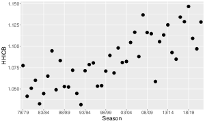
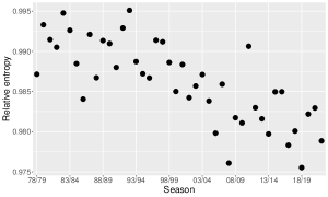
(a)	(b)

Figure 1: (a) The Herfindahl–Hirschman index of competitive balance (HHICB) is plotted for each season. This illustrates a general trend that HHICB is increasing over time and so consistent with the notion that the Premier League has become more imbalanced over time. (b) Relative entropy is plotted for each season. Here high values of relative entropy correspond to more balanced league and this plot suggests that the Premier League is gradually becoming more imbalanced over time.

2.3 The proposed statistical modelling approach

Each of the two measures of competitive balance outlined in the previous sections are somewhat limited as it is not straightforward to make any qualitative conclusions such as whether a season is balanced. Moreover, if there is evidence to suggest that a season is imbalanced, it would be useful to give an indication as to the nature of this imbalance, for example, which teams, if any, are stronger than the rest. To date, to the best of our knowledge, there is no literature which provides such a statistical framework. We aim to address this shortcoming here and develop a fully probabilistic model of competitive balance using a stochastic block modelling framework. The proposed network model offers multiple outcomes with information about the quality of the leagues and the relative competitiveness. Generally, the method we propose is more computationally demanding but richer in terms of results and inference we obtain from the final output it offers. Essentially the idea, which we now develop, is based on a statistical model which probabilistically partitions teams into blocks (or clusters) where the outcome (a win, draw or loss) for the home team follows the same multinomial probability mass function when any two teams in the same block play one another. Similarly, the outcome when any two teams which belong to different blocks play one another follows a multinomial probability mass function whose parameters depend on the blocks to which each team belong. In this way if we estimate that a single cluster (consisting of all teams) is most probable, then this provides evidence that the league is balanced. Moreover, in the case where the model estimates support for a league with more than one cluster, we assign probabilities of membership (or allocation) for each team to any of the blocks. This in turn would allow one to assess the presence of blocks or clusters of teams which are broadly competitive with each other. Additionally, by integrating over the uncertainty in the number of blocks we can estimate the number of teams in the strongest block and this provides another means to assess competitive balance. This perspective is particularly important for seasons in which there is broadly equal support for a one or a two block model, hence accounting for this uncertainty is an important factor to accommodate. Assessing the constituent teams in the strongest block of teams over time is of interest in the context of the English Premier League as there is anecdotal evidence of the emergence of a big-six block of teams over the past decade or so, namely, a collection of teams which are stronger than the remaining teams leading to a competitively imbalanced league. Our work aims to provide Bayesian framework to tackle these types of questions.

3 Representing the outcome for a season as a results matrix

To begin, we introduce the format of the data which we analyse each season. In particular, we represent the entire collection of results for every game in a single season in the form of a matrix. Here we consider the typical league scenario where each team plays every other team twice, once at home and once away from home. Therefore in a league with $N$ teams, there are $N\times(N-1)$ fixtures. The results of all these fixtures can be summarised in a $N\mathsf{x}N$ matrix, $R$. Each cell $r_{ij}$ contains the result of team $i$ playing against team $j$ when team $i$ plays at home. Clearly, the diagonal entries are missing as no team plays against itself. The matrix for the season $2021/22$ is displayed in Figure 2 (a).

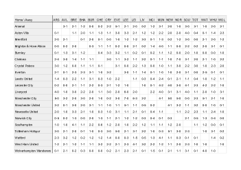
(a)	(b)

Figure 2: The matrix of results of the 2021/22 Premier League season. (a) Cell entries correspond to the result when a home team (row) plays an away team (column). (b) The results in (a) summarised in a results matrix by categorising each result as a win, draw or loss corresponding to the colour green, yellow or red, respectively.

In the modelling framework considered in this paper we take as outcome variable for every game, the three categorical variables, "win", "draw" or "loss" for the home team, denoted by $1,2$ or $3$, respectively. Therefore this leads us to summarise the matrix $R$ with a transformed matrix $\bm{y}$ which we term a results matrix,

$$\bm{y}=\begin{pmatrix}-&y_{12}&\dots&y_{1j}&\dots&y_{1N}\\ y_{21}&-&\dots&y_{2j}&\dots&y_{2N}\\ \dots&\dots&-&\dots&\dots\\ y_{i1}&y_{i1}&\dots&-&\dots&y_{iN}\\ \dots&\dots&\dots&\dots&-&\dots\\ y_{N1}&y_{N2}&\dots&y_{Nj}&\dots&-\end{pmatrix}\,,$$ (1)

where $y_{ij}\in\{1,2,3\}$, for $i=1,\dots,N;\quad j=1,\dots,N;j\neq i.$ The categorical outcomes for season $2021/22$ are displayed in Figure 2 (b), where the categorical variables "win", "draw" or "loss" are displayed using the colours green, yellow and red, respectively.

We remark that the results matrix $\bm{y}$ can be considered as an adjacency matrix of a directed network where each node represents a team and the outcome of a match between home team $i$ and away team $j$ is represented by the weight of the edge $y_{ij}$, where the weight takes a value in the set $\{1,2,3\}$. In many networks, we observe sparsity in the relational variable. For example, in a social network where the dyadic relational variable is binary, for instance a friendship relationship recorded as $1$ if the two nodes are friends, and $0$ otherwise, typically most dyads will take the value $0$. However this is not the case here as we always record a categorical outcome between each pair of nodes in the network. Hence, the network under study is dense and complete but does not allow self-loops.

4 A modification of the stochastic block model

The stochastic block model (SBM) of Nowicki and Snijders (2001) has proven to be incredibly useful in the analysis of relational network data. The core idea of an SBM, which we make precise in the subsequent section, in the context of a binary network is to partition the nodes of the network into blocks such that the probability of an edge between any two nodes depends on an unobserved (or latent) variable assigning each node to one of $K$ blocks or clusters in the network. One of the contributions of this paper is to explain how this framework can be extended to the context of football results data by developing a Bayesian stochastic block model which can be applied to the results matrix illustrated in the previous section.

Note that the model which we develop falls within the general framework of Aicher et al. (2015) where a generalisation of an SBM is presented for edge weights drawn from a exponential family distribution. We also note that in common with the generative weighted SBM approach of Aicher et al. (2015) we consider the case where the observed network is fully observed and is dense. That is to say that all possible interactions between each pair of teams are observed as each season each pair of teams plays each other twice, at home and away.

4.1 Specification of the block model

As outlined before, the aim of our stochastic block model is to partition the $N$ teams in a league, into $K$ blocks in such a way that the probability of a win, draw or loss for the home team is, broadly speaking, similar when any two teams in the same block play against one and other. But equally, that the probability outcome between teams belonging to different blocks, that is, where any team from one block plays at home against another team from a different block also has a similar probability of a win, draw or a loss. Essentially we wish to model the following scenarios. Matches involving teams within a block tend to have similar outcomes, while matches between teams from different blocks tend also to have similar outcomes. Crucially, the probability of a given outcome depends on the blocks to which each team is assigned. One of the key objectives is to infer the most likely value of $K$. In particular, if we deem that $K=1$ has most support, then we have some evidence that the league is balanced.

Here we develop the model and introduce some notation. We interchangeably use the terms nodes and teams, as from before there is an analogy between $\bm{y}$, the results matrix (1), and an adjacency matrix of a network. We make two main assumptions:

• For a $K$ block (or cluster) model, each node (or team), $i$ for $i=1,\dots,N$, belongs to one of the blocks with membership or allocation label, $z_{i}\in\{1,\dots,K\}$.

• The distribution of the relational structure $\bm{y}=(\bm{y_{ij}})_{1\leq i\neq j\leq N}$ is assumed to be conditionally independent given the latent variable of cluster memberships, $\bm{z}:=(z_{1},\dots,z_{N})$.

We now describe the various elements of our model.

Distribution for the allocation vector $\bm{z}$:

We assume that the entries of $\bm{z}$ are independent and identically distributed following a multinomial distribution:

$$z_{i}|\bm{\theta},K\stackrel{{\scriptstyle iid}}{{\sim}}Multi(1,\bm{\theta}=(\theta_{1},\theta_{2},\ldots,\theta_{K})),\ \text{for}\ i=1,\ldots,N,$$ (2)

where $P(z_{i}=k|\bm{\theta},K)=\theta_{k}$ is the probability that node $i$ belongs to cluster $k$, $\theta_{k}>0,\ k=1,\ldots,K$ and $\scriptstyle\sum_{k=1}^{K}\theta_{k}=1.$ We can write this probability mass function compactly as:

$$p(z_{i}|\bm{\theta},K)=\prod_{k=1}^{K}\theta_{k}^{I\left(z_{i}=k\right)},$$

where $I(A)$ is the indicator function $I$ defined as $1$ if condition $A$ is satisfied and $0$ otherwise. Thus, the distribution of the partition of the $N$ nodes into $K$ clusters conditional on $\bm{\theta}=(\theta_{1},\theta_{2},\ldots,\theta_{K})$ is:

$$\pi(\bm{z}|\bm{\theta},K)=\prod_{i=1}^{N}Multi(z_{i};1,\bm{\theta})=\prod_{i=1}^{N}\prod_{k=1}^{K}\theta_{k}^{I\left(z_{i}=k\right)}.$$ (3)

Prior for $\bm{\theta}$:

We assume a vague conjugate prior for the vector $\bm{\theta}$ following a Dirichlet distribution of dimension $K$ with vector of concentration parameters $\bm{\gamma}$:

$$\bm{\theta}|K\sim Dir(\bm{\gamma}=(\gamma_{1},\gamma_{2},\ldots,\gamma_{k},\ldots,\gamma_{K})).$$

We choose to set all concentration parameters to the same value, thus resulting in a symmetric prior. In particular, we set all $\gamma_{k}$’s equal to $\gamma_{0}=1$ yielding a uniform prior. Another possibility would be to set $\gamma_{0}=\frac{1}{2}$ corresponding to a non informative Jeffrey’s prior.

Blocks interaction probabilities:

Following the stochastic block model framework, the relational pattern of the nodes depends on the block probabilities of each game outcome. The $K\times K\times 3$ array, $\bm{p}$, encoding the block interaction probabilities is therefore of the form:

$$\bm{p}=\begin{pmatrix}\underline{p}^{11}&\underline{p}^{12}&\dots&\underline{p}^{1l}&\dots&\underline{p}^{1K}\\ \underline{p}^{21}&\underline{p}^{22}&\dots&\underline{p}^{2l}&\dots&\underline{p}^{2K}\\ \vdots&\vdots&\ddots&\vdots&\ddots&\vdots\\ \underline{p}^{k1}&\underline{p}^{k2}&\dots&\underline{p}^{kl}&\dots&\underline{p}^{kK}\\ \vdots&\vdots&\ddots&\vdots&\ddots&\vdots\\ \underline{p}^{K1}&\underline{p}^{K2}&\dots&\underline{p}^{Kl}&\dots&\underline{p}^{KK}\\ \end{pmatrix}$$

where,

$$\underline{p}^{kl}=(p_{1}^{kl},p_{2}^{kl},p_{3}^{kl})\;\;\mbox{and}\;\;\sum_{\omega=1}^{3}p_{\omega}^{kl}=1,$$

for all $k=1,\dots,K$ and $l=1,\dots,K$. In other words, $p_{1}^{kl},p_{2}^{kl}$ or $p_{3}^{kl}$ is the probability that a team allocated to block $k$ playing at home against a team allocated to block $l$, wins, draws or loses, respectively. Therefore, the random variable denoting the result (win, draw or loss) for any given team in block $k$ playing at home against any team in block $l$, playing away, has the same probability mass function $\underline{p}^{kl}$.

Distribution of the relational pattern of $\bm{y}$:

As in (Nowicki and Snijders, 2001), we model the distribution of edges between nodes conditionally on the block memberships. Additionally, we model that edges between nodes are identically distributed with parameters given by the interaction matrix $\bm{p}$. In contrast to (Côme and Latouche, 2015), where a Bernoulli distribution is chosen, the dyadic relation in our scenario takes categorical values. Here we model the observation $y_{ij}$ conditional on the latent allocations $z_{i},z_{j}$ as a multinomial distribution,

$$f(y_{ij}|z_{i},z_{j},\bm{p},K) = \prod_{k=1}^{K}\prod_{l=1}^{K}Multi(y_{ij};1,\underline{p}^{kl})^{I{\left(z_{i}=k\right)I\left(z_{j}=l\right)}}$$

$$= \prod_{k=1}^{K}\prod_{l=1}^{K}\left\{\prod_{\omega=1}^{3}\left(p_{\omega}^{kl}\right)^{I(y_{ij}=\omega)}\right\}^{I{\left(z_{i}=k\right)I\left(z_{j}=l\right)}}$$

for $i,j=1,\dots,N$, $i\neq j$.

Thus, given the latent structure $\bm{z}$, the block interactions array $\bm{p}$ and $K$, we can write the likelihood of the relational pattern $\bm{y}$ as

$$f(\bm{y}|\bm{z},\bm{p},K) = \prod_{i=1}^{N-1}\prod_{\underset{j\neq i}{j=1}}^{N}f(y_{ij}|z_{i},z_{j},\bm{p},K)$$ (4)

$$= \prod_{i=1}^{N-1}\prod_{\underset{j\neq i}{j=1}}^{N}\prod_{k=1}^{K}\prod_{l=1}^{K}\left\{\prod_{\omega=1}^{3}\left(p_{\omega}^{kl}\right)^{I(y_{ij}=\omega)}\right\}^{I{\left(z_{i}=k\right)I\left(z_{j}=l\right)}}.$$

Prior for the block interaction probabilities:

We assume that the entries of $\bm{p}$ are mutually independent and that each $\underline{p}^{kl}$ follows a conjugate prior from a 3-dimensional Dirichlet distribution:

$$\underline{p}^{kl}\sim Dir(\bm{\beta}=(\beta_{1},\beta_{2},\beta_{3})),\quad\mbox{for}\;\;k=1,\dots,K,\quad\mbox{and}\;\;l=1,\dots,K.$$

We set all the hyperparameters $\beta_{1},\beta_{2},\beta_{3}$ to $1$ leading to a uniform distribution.

Prior for $K$:

We treat the number of blocks or clusters as a random variable and choose a probability mass function for $K$ which is distributed as a zero-truncated Poisson random variable with $\lambda=1$ restricted to $1\leq k\leq K_{max}$, where $K_{max}$ is a user specified upper limit on the plausible number of blocks. We note that the justification for this prior was developed in (Nobile, 2005) in the context of mixture models and used in several papers including (Nobile and Fearnside, 2007), (Wyse and Friel, 2012) and (Geng et al., 2019). It consists of a Poisson distribution with rate parameter equal to $1$ conditioned on $K>0$:

$$K\sim Poi(1|K>0),$$

that is,

$$\pi(K|K>0)=\frac{Poi(1)}{1-Poi(K=0)}=\frac{1}{K!(e-1)}.$$ (5)

Therefore this prior probability mass function is proportional to $\frac{1}{K!}.$ As such, this prior reflects the fact that an SBM with $K$ block contains $K!$ permutations of the block labels, due to the label switching phenomena which is well understood for finite mixture models. This prior therefore assigns equal prior mass to each of these $K!$ possible relabellings. We return to the issue of label switching in Section 5.4. Note that we also explore the case of a discrete uniform prior on $K$ between $1$ and a user specified $K_{max}$. We detail the results of this analysis in application to the English first division/ Premier league in the supplementary material and show that the qualitative results remain largely unchanged compared to using truncated Poisson prior above.

4.2 Collapsing the stochastic block model

Following the specification of stochastic block model, we can write out the full joint posterior distribution of all model parameters as

$$\pi(\bm{z},\bm{p},\bm{\theta},K|\bm{y})\propto f(\bm{y}|\bm{p},\bm{z},K)\pi(\bm{p}|K)\pi(\bm{z}|\bm{\theta},K)\pi(\bm{\theta}|K)\pi(K).$$ (6)

Our interest here is primarily the joint posterior distribution of the latent allocation vector and number of blocks, $\pi(\bm{z},K|\bm{y})$. By virtue of the fact that we have chosen a conjugate prior for $\bm{\theta}$ and $\bm{p}$ we can integrate out both of these vectors from the posterior distribution yielding a collapsed posterior distribution,

$$\pi(\bm{z},K|\bm{y}) =\int_{\Theta}\int_{\bm{P}}f(\bm{y}|\bm{p},\bm{z},K)\pi(\bm{p}|K)\pi(\bm{z}|\bm{\theta},K)\pi(\bm{\theta}|K)\pi(K)d\bm{\theta}d\bm{p}$$

$$=\int_{\bm{P}}f(\bm{y}|\bm{p},\bm{z},K)\pi(\bm{p}|K)d\bm{p}\times\int_{\Theta}\pi(\bm{z}|\bm{\theta},K)\pi(\bm{\theta}|K)d\bm{\theta}\times\pi(K)$$ (7)

$$=f(\bm{y}|\bm{z},K)\pi(\bm{z}|K)\pi(K).$$

Details of the integration carried out in (7) are explained in Appendix A. Following (21) and (24) the collapsed posterior of the model has the form:

$$\pi(\bm{z},K|\bm{y})\propto\prod_{k=1}^{K}\prod_{l=1}^{K}\Gamma(3)\frac{\prod_{\omega=1}^{3}\Gamma(N_{kl}^{\omega}+1)}{\Gamma(\sum_{\omega=1}^{3}\left(N_{kl}^{\omega}+1)\right)}\cdot\prod_{k=1}^{K}\Gamma(n_{k}+1)\frac{\Gamma(K)}{\Gamma(N+K)}\times\frac{1}{K!},$$ (8)

where we define

$$N_{kl}^{\omega}=\sum_{i=1}^{N-1}\sum_{\underset{j\neq i}{j=1}}^{N}{I(y_{ij}=\omega)I\left(z_{i}=k\right)I\left(z_{j}=l\right)},$$

for $\omega=1,2,3$ and for $k,=1,\dots,K$ and $l,=1,\dots,K$, therefore allowing for the possibility that $k=l$. Also,

$$n_{k}=\sum_{i=1}^{N}{I\left(z_{i}=k\right)},\ k=1,\ldots,K.$$

Therefore $N_{kl}^{\omega}$ counts the number of times that the outcome $\omega$ was observed for all games involving a team allocated to block $k$ playing at home against a team allocated to block $l$. While $n_{k}$ accounts for the number of nodes/teams allocated to block $k$.

5 Bayesian estimation of the stochastic block model

Over time, many inferential strategies have been developed for the stochastic block model and its variants. For example, variational Bayes EM algorithm or integrated likelihood variational Bayes (Latouche et al., 2012). Moreover, model selection criteria based on the integrated complete likelihood (Biernacki et al., 2000) have been developed for bipartite and binary networks (Rastelli et al., 2018). Additionally, McDaid et al. (2013) developed a novel MCMC algorithm for an SBM for a network with binary edges and this is the framework which we develop here for our model.

The overall objective is to develop an algorithm to sample from the posterior distribution $\pi(\bm{z},K|\bm{y})$ (8). In so doing, this will allow us to estimate the posterior distribution of the number of blocks, $\pi(K|\bm{y})$, but also to estimate the posterior distribution $\pi(\bm{z}|K,\bm{y})$, so that we can assign probabilities to the allocation of teams to each of $K$ blocks. We also highlight, similar to Nobile and Fearnside (2007) that although our objective is to estimate the posterior distribution of $K$, we do not require a dimension changing MCMC algorithm such as reversible jump MCMC. This is because the dimension of the model is encoded in the vector $\bm{z}$ which is of fixed dimension $N$. We note that this strategy has also been employed in Wyse and Friel (2012) in the context of the latent block model.

We now describe the MCMC algorithm used to sample from (8), the posterior distribution $\pi(\bm{z},K|\bm{y})$. The algorithm is based on three move types:

Move type MK:

Metropolis move to insert or remove an empty cluster. This move changes the current state of $K$ but not the allocation vector $\bm{z}$.

Move type M-GS:

Metropolis-within-Gibbs move that updates all components of the allocation vector $\bm{z}$ but does not change the number of clusters.

Move type AE:

Metropolis-Hastings move to absorb or eject a cluster. This move affects both $\bm{z}$ and $K$.

We now present an overview of the pseudocode in Algorithm 1 before providing more details on each move type in turn.

Algorithm 1 MCMC algorithm to sample from $\pi(\bm{z},K|\bm{y})$.

1:We begin with an initial state $(\bm{z}^{1},K^{1})$.

2:while iteration $s<S$ do

3:     With equal probability select a move type MK, M-GS or AE.

4:     if MK is selected then:

5:         if an insert attempt is selected and accepted then

6:              $K$ is updated and increased by $1$ and an empty cluster is added

7:              $\bm{z}^{(s+1)}=\bm{z}^{(s)}$ and $K^{(s+1)}=K^{(s)}+1$          

8:         if a remove attempt is selected and accepted then

9:              $K$ is updated and decreased by $1$ and an empty cluster (if there is one) is removed.

10:              $\bm{z}^{(s+1)}=\bm{z}^{(s)}$ and $K^{(s+1)}=K^{(s)}-1$          

11:         otherwise

12:         The new state is set equal to the current state: $\bm{z}^{(s+1)}=\bm{z}^{(s)}$ and $K^{(s+1)}=K^{(s)}$      

13:     if M-GS is selected then:

14:         The value of $K$ is unchanged: $K^{(s+1)}=K^{(s)}$

15:         The allocation vector is updated to $\bm{z}^{(s+1)}$      

16:     if AE is selected then:

17:         With probability $p_{K}^{e}$ or $1-p_{K}^{e}$ select an absorption attempt or ejection attempt, respectively.

18:         if an absorption attempt is selected and accepted then

19:              $K^{(s+1)}=K^{(s)}-1$ and $\bm{z}$ is updated to $\bm{z}^{(s+1)}$          

20:         if an ejection attempt is selected and accepted then

21:              $K^{(s+1)}=K^{(s)}+1$ and $\bm{z}$ is updated to $\bm{z}^{(s+1)}$.          otherwise

22:         $\bm{z}^{(s+1)}=\bm{z}^{(s)}$ and $K^{(s+1)}=K^{(s)}$      

5.1 Move-type MK

When this move is chosen, the algorithm selects with probability $0.5$ to increase or decrease the number of clusters by inserting or deleting an empty cluster, respectively. In the case of an insert proposal, an empty cluster is added and the label with smallest value available is set to this cluster. This move is accepted with probability (9). When the current number of clusters $K$ is equal to the maximum allowed, $K_{max}$, an insert proposal is rejected with probability $1$ and the number of clusters remains at $K=K_{max}$. When proposing to delete a cluster, the algorithm first checks if some clusters are empty and the cluster with highest label value is selected. This move is accepted with probability (10). Otherwise, if $K=1$, the proposal to delete a cluster is rejected and the number of clusters remains at $K=1$. Notice that the move-type MK affects $K$ but leaves the allocation vector $\bm{z}$ unchanged. If the proposal to insert an empty cluster is accepted, there will be an additional label but no nodes will be assigned to this new cluster. In case of a remove proposal, the number of clusters decreases, but again the allocation vector $\bm{z}$ will remain unchanged. Below we provide an algorithmic description of this move type. For more details of the derivation of the acceptance probabilities below, see Appendix B.1.

At iteration $s$ with current state $(\bm{z}^{(s)},K^{(s)})=(\bm{z},K)$:

1. An insertion or a removal of an empty cluster is proposed with probability $0.5$.

2. If the insertion attempt is selected:
   

   • If $K=K_{max}$, the new state is set equal to the current state: $K^{(s+1)}=K_{max}$.

   • If $K<K_{max}$, we accept $K^{(s+1)}=K+1$ as the new state with acceptance probability: $min\left[1,\alpha\right]$, where:

     $$\alpha=\frac{K}{(N+K)(K+1)}$$ (9)

3. If the delete attempt is selected:
   

   • If $K=1$, the new state is set equal to the current state: $K^{(s+1)}=1$.

   • If $K>1$, we always accept $K^{(s+1)}=K-1$ as the new state since the acceptance probability in this case is $min\left[1,\alpha\right]$, where:

     $$\alpha=\frac{K(N+K-1)}{K-1},$$ (10)

     which is always greater than $1$. In other words, we automatically accept the proposal to delete an empty cluster, if there is one.

Notice that in all cases the new state for $\bm{z}^{(s+1)}$ will be equal to the current state $\bm{z}^{(s)}$.

5.2 Move-type M-GS

This move-type involves a standard Metropolis-within-Gibbs update of each element of the allocation vector $\bm{z}$. This sweep consists of updating the allocation of each node sequentially from $z_{1}$ through to $z_{N}$. Recall that this move-type does not change the current value of $K$. We describe this move type below and provide details of the calculation involved in (11) in Appendix B.2 .

At iteration $s$, we carry out a sweep of $\bm{z}^{(s)}$ yielding an updated allocation vector $\bm{z}^{(s+1)}=(z_{1}^{(s+1)},z_{2}^{(s+1)},\ldots,z_{N}^{(s+1)})$. To do this, we update each element $z_{i}$ of $\bm{z}^{(s)}$ using a Metropolis kernel, for $i=1,\dots,n$, as follows:

1. Set $\bm{z}^{(s+1)}=\bm{z}^{(s)}$.

2. For $\{i=1,\dots,n\}$

   1. Suppose the current state of $z^{(s)}_{i}=k_{0}$. Propose a new state $z_{i}^{\prime}$ for $z^{(s)}_{i}$ by sampling a new cluster label uniformly from the set $\{1,\dots,K\}\setminus k_{0}$.

   2. Denote the proposed new allocation vector as $\bf{z}^{\prime}$, which is identical to the current state of the allocation vector, $\bm{z}^{(s+1)}$, except for its $i$th element, which is $z_{i}^{\prime}$.

   3. The proposed new allocation vector $\bf{z}^{\prime}$ is accepted with probability

      $$\alpha=\min\left(1,\frac{\pi(\bm{z}^{\prime},K|\bm{y})}{\pi(\bm{z}^{(s+1)},K|\bm{y})}\right)$$ (11)

      in which case, $z^{(s+1)}_{i}=z_{i}^{\prime}$. Otherwise, $z^{(s+1)}_{i}=z^{(s)}_{i}$.

5.3 Move-type AE

This move was originally proposed in Nobile and Fearnside (2007) and is designed to allow a change to the number of blocks, $K$ as well as to the allocation vector $\bm{z}$. It consists of a Metropolis-Hastings pair of absorption/ejection moves. Here we choose to attempt an ejection with probability $p_{K}^{e}$, depending on the current number of blocks. In particular we set,

$$p_{K}^{e}=\begin{cases}1,\text{ if }K=1,\\ 1/2,\text{ if }1<K<K_{max},\\ 0\ ,\text{ if }K=K_{max}.\end{cases}$$

Otherwise, an absorption move is proposed.

Ejection attempt

A block $j_{1}$ is randomly selected as the ejecting block among the $K$ available blocks. The ejected block is assigned the label $j_{2}=K+1$. Each of the nodes in the block $j_{1}$ are then randomly assigned to a new block $j_{2}$ or remain in the original block $j_{1}$. The probability for each node to be allocated to the new block $j_{2}$, that is the probability of a node to be ejected, is constant and indicated with $p_{E}$, where $p_{E}\sim U(0,1)$. Note, that instead of specifying an ejection probability $p_{E}$, we integrate over the $p_{E}$ in much the same manner as collapsing. The details of this are outlined in Appendix B.3.

Absorption attempt

Here both the absorbing and absorbed block, $j_{1}$ and $j_{2}$, respectively, are randomly chosen from the $K$ available labels. All nodes allocated in block $j_{2}$ are reallocated to block $j_{1}$.

This move type, as pointed out in Nobile and Fearnside (2007), leads to improved mixing. Reversibility requires that the ejected block is a random draw from the resulting $K+1$ clusters. To achieve this, at the end of the ejection move we perform a swap between the label $j_{2}=K+1$ and a randomly selected label from the set of all available ones, $\mathcal{K^{\prime}}=\{1,2,\ldots,K+1\}$. The candidate state $(\bm{z}^{\prime},K^{\prime})$ is accepted with probability min$(1,\alpha)$, where $\alpha$ is the product of the joint probability ratio and the proposal ratio as detailed below.

We detail the proposal ratios and probabilities for the ejection and absorption moves below. We refer the reader to Appendix B.3 for precise details of the derivation of these quantities.

The ratio of posterior densities for ejection attempt is:

$$\frac{P_{prop}((\bm{z}^{\prime},K^{\prime})\rightarrow(\bm{z},K))}{P_{prop}((\bm{z},K)\rightarrow(\bm{z}^{\prime},K^{\prime}))}=\frac{(1-p_{K}^{e})}{p_{K}^{e}}\cdot(n_{j_{1}}+n_{j_{2}}+1),$$ (12)

where,

$$n_{j_{1}} =\sum_{i=1}^{N}I(z^{\prime}_{i}=j_{1})\text{ is the number of nodes in the ejecting cluster after reallocation,}$$

$$n_{j_{2}} =\sum_{i=1}^{N}I(z^{\prime}_{i}=j_{2})\text{ is the number of nodes in the ejected cluster.}$$

To obtain $\alpha$, we multiply (12) by:

$$\frac{\pi(\bm{z}^{\prime},K^{\prime}|\bm{y})}{\pi(\bm{z},K|\bm{y})}=\frac{\prod_{k=1}^{K+1}\prod_{l=1}^{K+1}\Gamma(3)\frac{\prod_{\omega=1}^{3}\Gamma(N_{kl}^{{}^{\prime}\omega}+1)}{\Gamma(\sum_{\omega=1}^{3}\left(N_{kl}^{{}^{\prime}\omega}+1)\right)}\times\prod_{k=1}^{K+1}\Gamma(n^{\prime}_{k}+1)}{\prod_{k=1}^{K}\prod_{l=1}^{K}\Gamma(3)\frac{\prod_{\omega=1}^{3}\Gamma(N_{kl}^{\omega}+1)}{\Gamma(\sum_{\omega=1}^{3}\left(N_{kl}^{\omega}+1)\right)}\times\prod_{k=1}^{K}\Gamma(n_{k}+1)}\cdot\frac{K}{(N+K)(K+1)}$$ (13)

and accept this move with probability $\min(1,\alpha)$.

For the absorption attempt the proposal ratio takes the form:

$$\frac{P_{prop}((\bm{z}^{\prime},K^{\prime})\rightarrow(\bm{z},K))}{P_{prop}((\bm{z},K)\rightarrow(\bm{z}^{\prime},K^{\prime}))}=\frac{p_{K}^{e}}{(1-p_{K}^{e})}\cdot\frac{1}{(n_{j_{1}}+n_{j_{2}}+1)}.$$ (14)

The corresponding posterior density ratio appears as:

$$\frac{\pi(\bm{z}^{\prime},K^{\prime}|\bm{y})}{\pi(\bm{z},K|\bm{y})}=\frac{\prod_{k=1}^{K-1}\prod_{l=1}^{K-1}\Gamma(3)\frac{\prod_{\omega=1}^{3}\Gamma(N_{kl}^{{}^{\prime}\omega}+1)}{\Gamma(\sum_{\omega=1}^{3}\left(N_{kl}^{{}^{\prime}\omega}+1)\right)}\times\prod_{k=1}^{K-1}\Gamma(n^{\prime}_{k}+1)}{\prod_{k=1}^{K}\prod_{l=1}^{K}\Gamma(3)\frac{\prod_{\omega=1}^{3}\Gamma(N_{kl}^{\omega}+1)}{\Gamma(\sum_{\omega=1}^{3}\left(N_{kl}^{\omega}+1)\right)}\times\prod_{k=1}^{K}\Gamma(n_{k}+1)}\cdot\frac{K(N+K-1)}{K-1}.$$ (15)

Once again, $\alpha$ is then the product of (14) and (15) and the move is accepted with probability $\min(1,\alpha)$.

5.4 Label switching phenomenon and correction

In the framework outlined above, the discrete labels in the allocation vector $\bm{z}$ are not identifiable by the model. This is because the likelihood is invariant to permutations of the labels of $\bm{z}$, leading to the well-known label switching phenomenon. This scenario arises naturally when using MCMC methods and, as a result, it is necessary to employ an algorithm to correct for this. In particular we use the online relabelling algorithm proposed in Nobile and Fearnside (2007) which relies on the algorithm of Carpaneto and Toth (1980) to correct the output of a sample from the posterior distribution of $\bm{z}$ from the MCMC algorithm described above. The relabeling algorithm which we use first orders this sample by the number of non-empty blocks in increasing order to yield an ordered sample $\bm{Z}:=\{\bm{z}^{(1)},\bm{z}^{(2)},\ldots,\bm{z}^{(S)}\}$. The algorithm then iterates over $\bm{Z}$ comparing the current allocation vector to all previously relabeled states. The current state is then relabeled by permuting its labels so that a distance to all the preceding relabeled states is minimised. Here we define a distance between any two allocation vectors, $\bm{z}$ and $\bm{z}^{\prime}$ as

$$D(\bm{z},\bm{z}^{\prime})=\sum_{i=1}^{N}I(z_{i}\neq z_{i}^{\prime}),$$ (16)

where $I$ is the usual indicator function used previously, so that this distance records the number of locations where the entries of $\bm{z}$ and $\bm{z}^{\prime}$ differ. Further, let $\sigma$ denote a permutation of the integers $1,\dots,K$, that is, a bijection from the set $\{1,\dots,K\}$ onto itself, and let $\sigma\bm{z}$ denote the relabeled allocation vector by applying the permutation to the labels of the vector $\bm{z}$. This algorithm was implemented using the R package collpcm and can be briefly described as follows:

1. The sample of $S$ allocation vectors from the MCMC algorithm are ordered by the number of non-empty blocks and in decreasing order with respect to the number of labels used yielding an sequence of allocation vectors $\{\bm{z}^{(1)},\bm{z}^{(2)},\ldots,\bm{z}^{(S)}\}$.

2. Set $\sigma^{(1)}$ to be the identity permutation.

3. For $\{s=2,\dots,S\}$
   Find the permutation $\sigma^{(s)}$ which minimises the sum of distances from the permuted allocation vector $\bm{z}^{(s)}$ to all preceding permuted allocation vectors,

   $$\sigma^{(s)}=\arg\min_{\sigma}\sum_{t=1}^{s-1}D(\sigma\bm{z}^{(s)},\sigma^{(t)}\bm{z}^{(t)}),$$

   where $D(\sigma\bm{z}^{(s)},\sigma^{(t)}\bm{z}^{(t)})$ is the distance function (16).

4. The relabeled sequence of allocation vectors

   $$\{\sigma^{(1)}\bm{z}^{(1)},\dots,\sigma^{(S)}\bm{z}^{(S)}\}$$

   is returned.

6 Analysis of over $40$ seasons of the English First Division/ Premier League

In this section, we present a detailed analysis for the 2021/22 Premier League season, highlighting some of the important aspects of the output from the model. In particular, for this season, the SBM partitioned the teams into two blocks where one can visually see structure within and between each block – namely that teams within each block are quite competitive while when a team plays another from a different block, the result usually favours the team from the strongest block. We then extend our analysis to each season over the past $44$ years from $1978/79$ to $2021/22$ encompassing the end of the old English First Division through to the inception of the Premier League. Analysing each season over this length of time will allow us to provide insights into changes in competitive balance. For each season, the MCMC algorithm described in Section 5 was run for $200,000$ iterations, discarding the first $50,000$ as burn-in iterations and took approximately $3$ minutes to complete. This was followed by the label switching correction algorithm which took only a few seconds to run. The MCMC algorithm was coded in R and a link to this code and the data used in this paper can be found here https://github.com/francescabasini/Football_SBM.

6.1 Analysis of the 2021/22 Premier League season

Here we present a detailed analysis of the $2021/22$ season as this provides us with the opportunity to discuss some of the salient features of our model. To begin we present in Figure 3 a summary of the outcome for each team in terms of the percentage of wins, draws and losses over the course of the season. As expected, this illustrates that teams that finish higher in the league tend to have more wins. While the opposite happens for teams which are placed lower in the league. It also illustrates the disparity in terms of percentage of wins (and losses) between teams with a high final position in the league compared to those whose final position was towards the bottom of the league.

As before, the data for this season is presented in Figure 4 (a) in the form of a results grid.

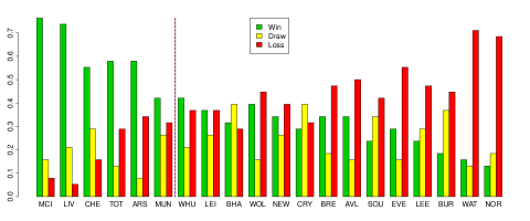
Figure 3: Barplot of the percentage of overall outcomes (win, draw, loss) for each team for Season 2021/22. Teams are listed in decreasing order from left to right according to their position in the final league table. The dotted line corresponds to where teams are separated into their most likely block.

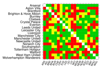
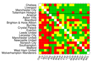
(a)	(b)

Figure 4: Match grid for the 2021/22 season. Each entry of this grid corresponds to a match where a home team (row entry) plays against an away team (column entry). The outcome of each match is represented using green, yellow and red colours corresponding to a win, draw and loss, respectively, for the home team. (a) Teams listed in alphabetical order. (b) Teams listed by most likely block membership, a posteriori. The solid horizontal and vertical lines (which also coincides with final league position) separates each team in their most likely block.

The MCMC algorithm 1 was implemented using each of the three moves types, MK, GS and AE following the description in Section 5. The posterior probability of $K=1$, $K=2$ and $K=3$ was estimated to be $0.0$, $0.97$ and $0.03$, respectively. This indicates that there is overwhelmingly most support, a posteriori, for a model with two blocks. While the posterior distribution of the allocation variable $\bm{z}$ conditional on $K=2$ indicates that the strongest block is comprised of Chelsea, Liverpool, Manchester City, Tottenham. We also also illustrate this in Table 1 by presenting the estimated posterior probability that each team belongs to the strongest block, conditional on $K=2$, together with the overall points total for each team at the end of the season.

Note that further output of the model for this season is presented in Appendix C of the supplementary material. We also note that permuting the rows and columns of the match grid matrix in Figure 4 (b) by final league position reveals the block structure of the results. Here the solid vertical and horizontal lines separate the two blocks of teams. We make the following remarks to illustrate some important features of the estimated block structure in Figure 4 (b). The top right quadrant corresponds to when a team in the strongest block plays at home against a team in the weakest block. Here the colours are predominately green, indicating that the home team generally won. While the bottom left quadrant corresponds to the opposite situation, when a team in the weakest block plays at home against a team in the strongest block. Here the colours are predominately red, indicating the away team (in the strongest block) generally won. Finally, note that the top left and bottom right quadrants, corresponds to the within-block matches for the strong block and weak blocks, respectively. Each block contains a reasonably balanced mix of all three colours, indicating that these teams were generally quite balanced.

	Points	$P(\mbox{top block}|\bm{y},K=2)$
Manchester City	93	1.00
Liverpool	92	0.99
Chelsea	74	0.88
Tottenham Hotspur	71	0.74
Arsenal	69	0.38
Manchester United	58	0.02
West Ham United	56	0.01
Leicester City	52	0.00
Brighton & Hove Albion	51	0.01
Wolverhampton Wanderers	51	0.01
Newcastle United	49	0.00
Crystal Palace	48	0.00
Brentford	46	0.00
Aston Villa	45	0.00
Southampton	40	0.00
Everton	39	0.00
Leeds United	38	0.00
Burnley	35	0.00
Watford	23	0.00
Norwich City	22	0.00

Table 1: Final league table for the Premier League Season 2021/22 showing the number of points for each team. For comparison, the estimated posterior probability of allocation of each team to the top block is also presented. The solid horizontal line separates the $4$ teams most likely to be in the top block, a posteriori.

6.1.1 Analysing the posterior distribution of $\underline{p}^{kk}$ to assess evidence of a home effect

It is possible to use the output of the model to infer the posterior distribution of $\bm{p}$ conditional on the latent allocation $\bm{z}$ and $K$. It particular, this allows us to address the question of whether there is an advantage to playing at home, by analysing the posterior distribution of the within block probability vector, $\underline{p}^{kk}$, for $k=1,\dots,K$. It is useful to do so, as teams within a block should be balanced and so any effect of playing at home should be more apparent. It turns out that this posterior distribution of $\bm{p}$ is proportional to the likelihood (given by equation (4) in the text),

$$\pi(\bm{p}|\bm{y},\bm{z},K)\propto\prod_{i=1}^{N-1}\prod_{\underset{j\neq i}{j=1}}^{N}\prod_{k=1}^{K}\prod_{l=1}^{K}\left\{\prod_{\omega=1}^{3}\left(p_{\omega}^{kl}\right)^{I(y_{ij}=\omega)}\right\}^{I{\left(z_{i}=k\right)I\left(z_{j}=l\right)}}.$$

In turn, this allows us to sample the within block multinomial probabilities, $\underline{p}^{kk}$ by conditioning on teams only allocated to block $k$. In the context of the $2021/22$ season, it turns out that since block $1$ consists of only $4$ teams, there are only $12$ games involving teams from this block of which there were $3$ home wins, $6$ draws and $3$ home losses. In turn, this is reflected in the inferred posterior distribution of $\underline{p}^{11}$ presented in Table 2 which shows that the posterior density for $p^{11}_{1}$ is identical to $p_{3}^{11}$. By contrast, block $2$ contains many more teams. From Table 2 we see that the posterior density of $p^{22}_{1}$ has a $95\%$ credible interval of $[0.36,0.49]$ which is much greater than the corresponding $95\%$ credible interval for $p^{22}_{3}$ which is estimated to be $[0.25,0.37]$. This indicates the presence of a home effects within this block of teams.

	mean	sd	$2.5\%$	$97.5\%$
$p_{1}^{11}$	0.26	0.11	0.08	0.50
$p_{2}^{11}$	0.47	0.12	0.24	0.71
$p_{3}^{11}$	0.27	0.11	0.09	0.50
$p_{1}^{22}$	0.42	0.03	0.36	0.49
$p_{2}^{22}$	0.27	0.03	0.22	0.33
$p_{3}^{22}$	0.31	0.03	0.25	0.37
$p_{1}^{12}$	0.75	0.05	0.64	0.84
$p_{2}^{12}$	0.13	0.04	0.06	0.22
$p_{3}^{12}$	0.12	0.04	0.05	0.21
$p_{1}^{21}$	0.15	0.04	0.08	0.24
$p_{2}^{21}$	0.16	0.05	0.08	0.26
$p_{3}^{21}$	0.69	0.06	0.57	0.79

Table 2: Posterior summaries (mean, standard deviation, $2.5$th and $97.5$th percentiles) of the multinomial probability vectors, $\underline{p}^{11}$, $\underline{p}^{22}$,$\underline{p}^{12}$ and $\underline{p}^{21}$, respectively.

Additionally, as one might expect, the posterior density for $\underline{p}^{12}$ indicates that the probability of a win, when a home team in block $1$ plays a team in block $2$, is very high, with a $95\%$ credible interval $[0.64,0.84]$. While the opposite is the case when a team in block $2$ plays at home against a team in block $1$. Here the $95\%$ credible interval for $p^{21}_{1}$ is $[0.08,0.24]$.

6.2 Analysis of four decades of the English first division/ Premier League

Here we extend our analysis to each season over the past $44$ years from $1978/79$ to $2021/22$. This period of time encompasses the end of the old English First Division and the inception of the Premier League in $1992/93$ and allows an examination of any changes in the competitive balance of the league. We begin by providing a summary of the output of our model for each season exploring the posterior probability of $K$ for each season. A summary of the output of our analysis on a season-by-season basis is presented in Table 3 where we displayed the estimated posterior probability for a one block model through to a four block model. We then extend this analysis in Section 6.2.1 to provide more detail on the block structure for each season by analysing the marginal posterior probability of allocation of teams to the strongest block. This allows us to explore how the number of teams in the strongest block has changed over time. In particular, in Section 6.3 we explore which teams have persisted in the strongest block over the past two decades of our study. This then facilitates an assessment of whether there is evidence to suggest that a big-six group of teams emerged over this time period.

Number of clusters Season 1 2 3 4 78/79 1.17 96.74 2.08 0.01 79/80 97.57 2.39 0.04 0.00 80/81 30.55 69.10 0.35 0.00 81/82 97.25 2.72 0.02 0.00 82/83 99.80 0.20 0.00 0.00 83/84 99.15 0.85 0.00 0.00 84/85 42.34 57.22 0.44 0.00 85/86 0.00 99.81 0.19 0.00 86/87 99.49 0.51 0.00 0.00 87/88 12.41 87.26 0.33 0.00 88/89 99.20 0.79 0.01 0.00 89/90 98.66 1.32 0.02 0.00 90/91 49.31 50.07 0.61 0.00 91/92 94.10 5.89 0.01 0.00 92/93 98.85 1.15 0.00 0.00 93/94 27.98 71.08 0.94 0.00 94/95 22.19 74.59 3.21 0.01 95/96 48.05 51.68 0.27 0.00 96/97 99.63 0.37 0.00 0.00 97/98 98.14 1.85 0.01 0.00 98/99 0.07 99.78 0.16 0.00 99/00 64.34 35.27 0.39 0.00

Number of clusters Season 1 2 3 4 00/01 88.26 11.06 0.68 0.00 01/02 0.13 99.37 0.49 0.01 02/03 59.29 40.19 0.52 0.01 03/04 6.45 88.39 5.12 0.04 04/05 0.00 99.79 0.21 0.00 05/06 0.15 97.08 2.73 0.04 06/07 5.45 92.37 2.17 0.01 07/08 0.00 93.81 5.92 0.27 08/09 0.00 99.24 0.76 0.00 09/10 0.00 95.30 4.67 0.03 10/11 79.87 20.09 0.05 0.00 11/12 1.68 96.91 1.40 0.02 12/13 0.00 99.64 0.36 0.00 13/14 0.00 98.96 1.04 0.00 14/15 7.30 88.70 3.98 0.03 15/16 75.37 24.38 0.25 0.00 16/17 0.00 98.99 1.01 0.00 17/18 0.00 97.95 2.03 0.02 18/19 0.00 97.94 2.04 0.02 19/20 2.10 96.47 1.41 0.01 20/21 15.86 81.85 2.25 0.04 21/22 0.04 96.58 3.35 0.03

Table 3: Posterior probability of $K$, expressed as a percentage, over the last $44$ seasons. The block model with highest posterior probability is coloured accordingly.

Overall, Table 3 indicates there was most support each season, a posteriori, for either a one block or a two block model, however the number of seasons where a two block model has most support, a posteriori, increases considerably over the past two decades. In particular, over the first half of this study period there is no strong support for either a one or a two block model. In fact for some seasons there is broadly equal posterior support for either model, for example, seasons $1984/85$, $1990/91$, $1995/96$. In fact, of note is season $1984/85$ where the second block consisted of a single team, Stoke City, who were bottom of the league in that season recording only $3$ wins from a possible $42$ matches. This situation changes considerably when we analyse the final two decades of this study. The right hand side of Table 3 indicates that there is typically most support from a two block model, but further that the posterior probability for a two block model is over $0.8$ for almost every season since $2003/04$, providing strong evidence that the league has become more competitively imbalanced since then. There are a few exceptions to this, most notably, season $2015/16$ when Leicester City famously won their first league title. However, in general, this analysis suggests a structural change in the nature of the competitiveness of the league since the turn of the millennium.

Additionally, there was quite limited support for a three block model, for example, from the beginning of the study until $2002/03$ almost all seasons presented very little, if any, posterior support for this model, with the exception of season $1994/95$, for which a three block model was attributed $0.03$ probability. Conversely, from $2003/04$ to the end of the study, there were some seasons which gave some modest support to a three block model. For example, in seasons $2003/04$, $2007/08$, $2009/10$, there was approximately $0.05$ posterior probability for this model. Again, this is consistent with the idea that the league was more imbalanced over the past two decades.

6.2.1 Marginal posterior allocation of a team to the strongest block

It is informative to estimate the marginal probability that a team belongs to the strongest block by integrating over the uncertainty in the number of blocks. This is particularly important for seasons where there is broadly equal support for a one or a two block model. For each value of $k$, post label switching we associate the block label $1$ with the strongest block of teams. We estimate the marginal posterior probability that team $i$ is in the strongest block averaging over all possible number of blocks as follows,

$$\pi(z_{i}=1|\bm{y}) = \sum_{k=1}^{K_{max}}\pi(z_{i}=1,K=k|\bm{y})$$ (17)

$$= \sum_{k=1}^{K_{max}}\pi(z_{i}=1|\bm{y},K=k)\pi(K=k|\bm{y}).$$

In Figure 5 we display the estimated marginal posterior allocation of each team to the strongest block following (17) for each season. Moreover, we again use the convention to colour each season according to the block model with most support (sand and blue corresponding to seasons in which a one block model or a two block model, respectively, has most support). Notice in Figure 5 that for seasons from $1978/79$ to around $2002/03$ the spread of posterior probability of allocation to the top block for each team is quite different to that of the seasons which follow. In particular, from $2003/04$ to $2021/22$ we see that there are typically a relatively large group of teams (in a two block season) which have very small posterior probability of being allocated to the strongest block, indicated in the bottom right hand corner of Figure 5. In other words, there is a strong separation of teams in terms of posterior allocation to the strongest block, compared to the first half of seasons in this study. In addition, we make the important remark that the number of teams allocated the strongest block for each of the seasons from $2003/04$ to $2021/22$, that is to say, those with high posterior probability of allocation to the strongest block, typically consists of a small number of teams. This analysis leads us in Section 6.3 to explore the composition of teams in the strongest block over the past two decades.

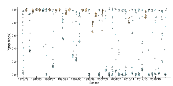
Figure 5: The posterior allocation probability of belonging to the strongest group of teams over the $44$ seasons under study. For each season the colour indicates whether the league was partitioned into a single cluster (sand colour) or two (light blue). Each point represents the estimated posterior probability of allocation for a team. Note that within each season the points have been jittered.

Following from the analysis presented above we can explore the number of teams estimated to belong to the strongest block, by again integrating over the uncertainty in $k$. To do this, we simply examine (17) for each team and investigate if this posterior probability is greater than $0.5$. If so, we assign this team to the strongest block of teams. For each season, this allows one to estimate the size of the strongest block of teams for each season in turn. This number serves as a useful alternative index of competitive balance for each season. This information is presented in Figure 6. We highlight for certain seasons that although a two block model has most posterior support, the estimated number of teams in the strongest block can be close to or equal to the total number of teams in the league that season. This is the case for seasons $1990/91$ and $1995/96$ where there was broadly equal posterior support for a one and a two block model, integrating over the uncertainty in the number of blocks indicates that all $20$ are estimated to be in the strongest block suggesting quite a balanced league for these seasons.

An overall analysis of Figure 6 indicates that the number of teams in the strongest block is quite large for the majority of seasons in the first half of the study period until around $2003/04$. From $1978/79$ to $2003/04$ the estimated size of the top block contained more than half the total number of teams in the league each season, ranging from $11$ to $22$ teams for $20$ out of $25$ season. This is in stark contrast with the seasons which followed, where the size of the top block ranged from $2$ to $8$ teams for $15$ out of $18$ season. A notable exception is season $2020/21$, where the size of top block was $15$ teams. In this season COVID-19 had an impact on the league, particularly through the absence of crowds for the majority of games in this season.

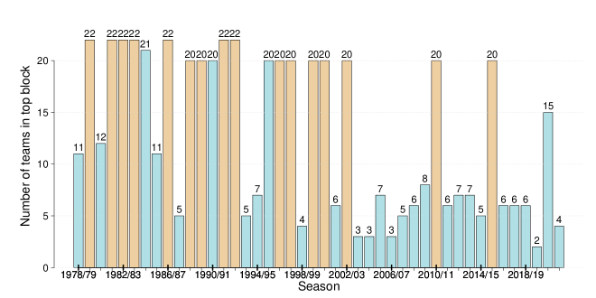
Figure 6: Barplot displaying the posterior estimate of the number of teams allocated to the strongest block each season. Single and two block seasons are coloured sand and blue, respectively. This illustrates that the size of the strongest block has generally decreased during the second half of the study period.

We supplement more detail to the analysis above in Figure 13 by displaying the posterior probability of allocation to the strongest block for each season for Arsenal, Chelsea, Liverpool, Manchester city, Manchester United, Tottenham Hotspur over the entire course of the study. This provides additional information by illustrating that the posterior probability of allocation to the strongest team can vary considerably for each team and over each season. For example, in $2017/18$ there is much less support for Arsenal’s inclusion in the strongest block (the estimated probability in this case turns out to be $0.63$).

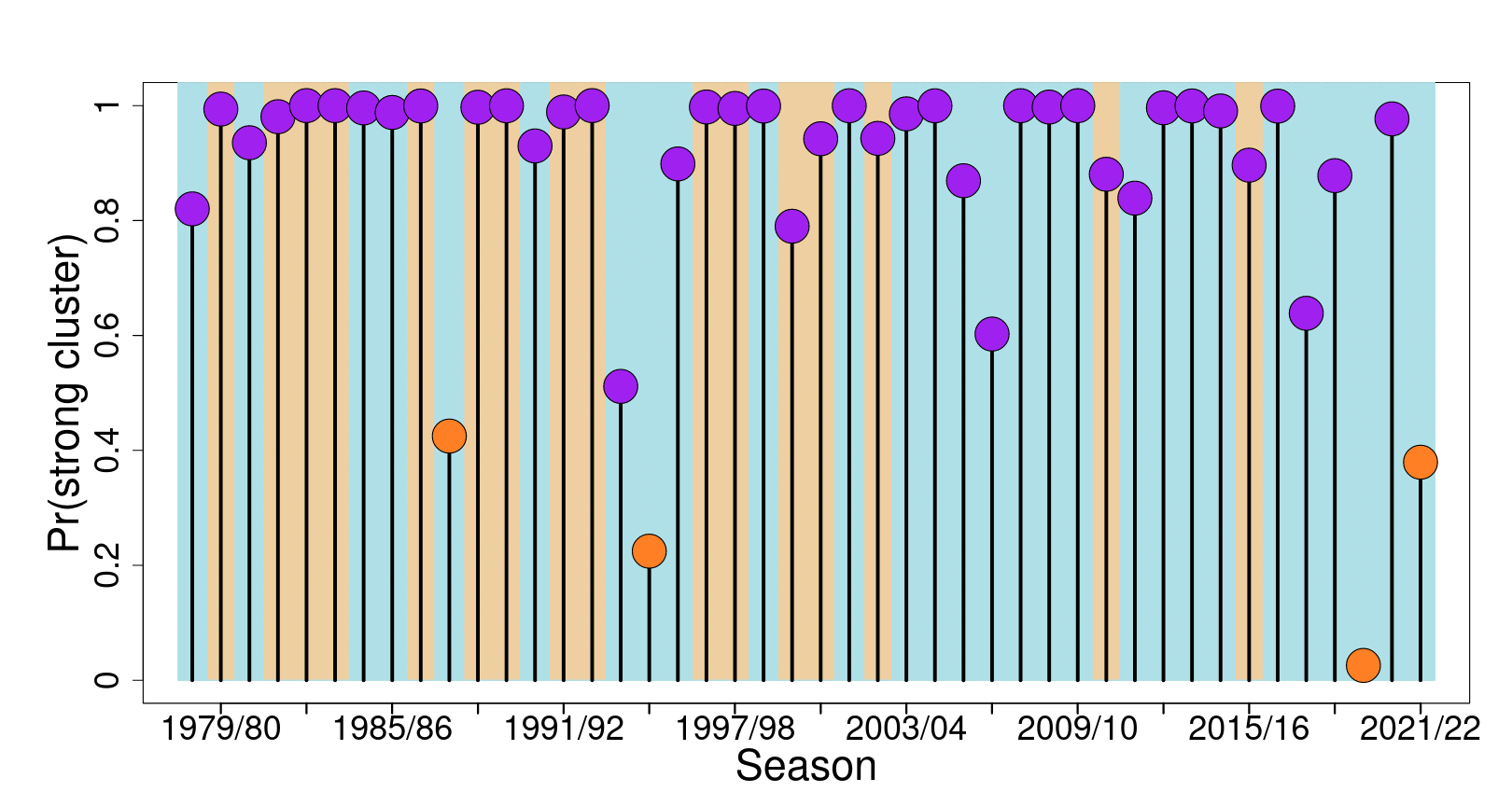
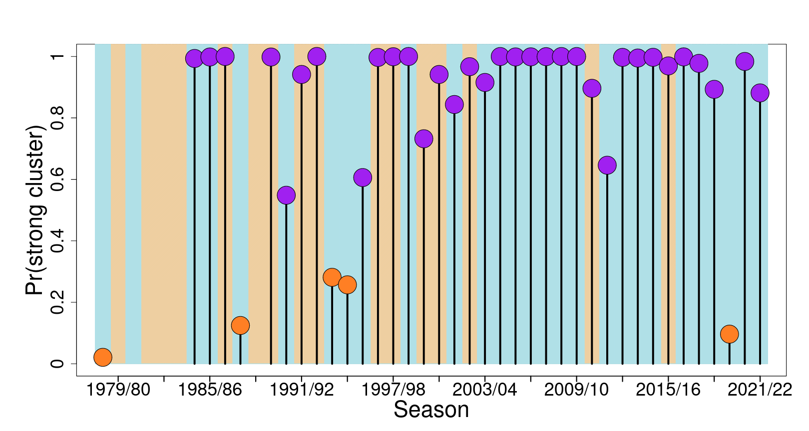
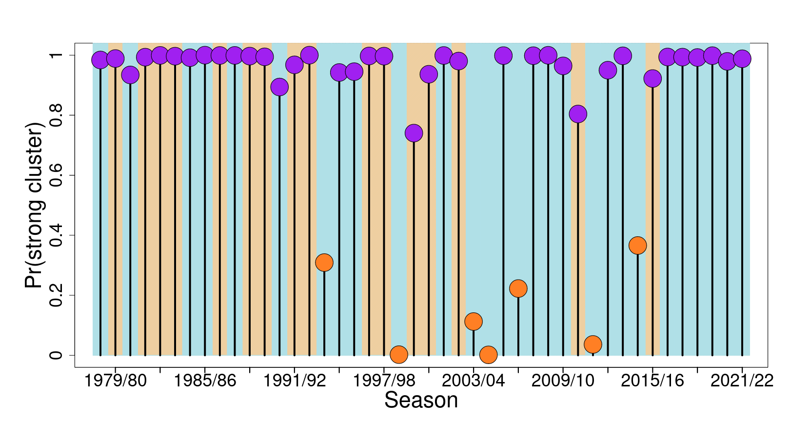
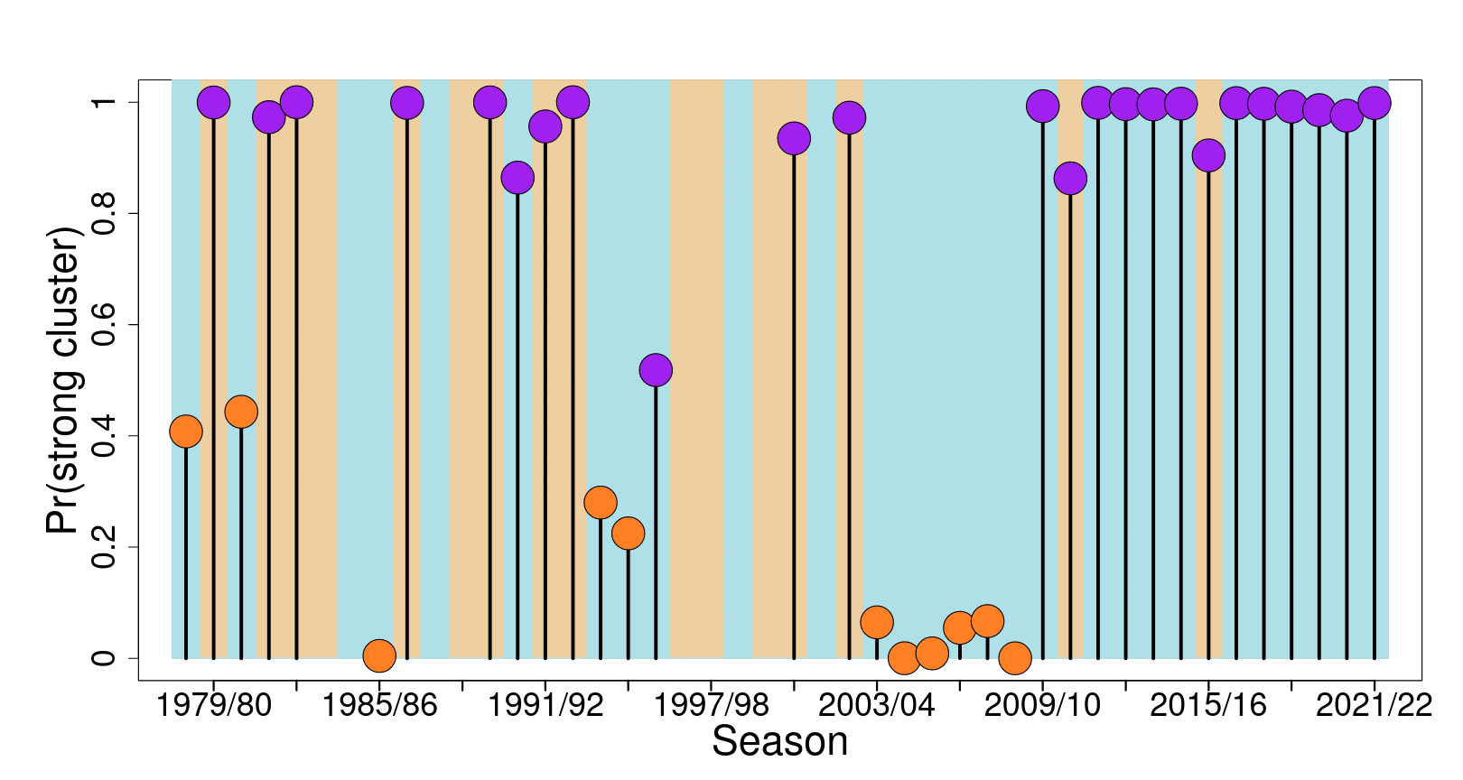
- figure [2] [] [] [2] [] [] [2] [] []

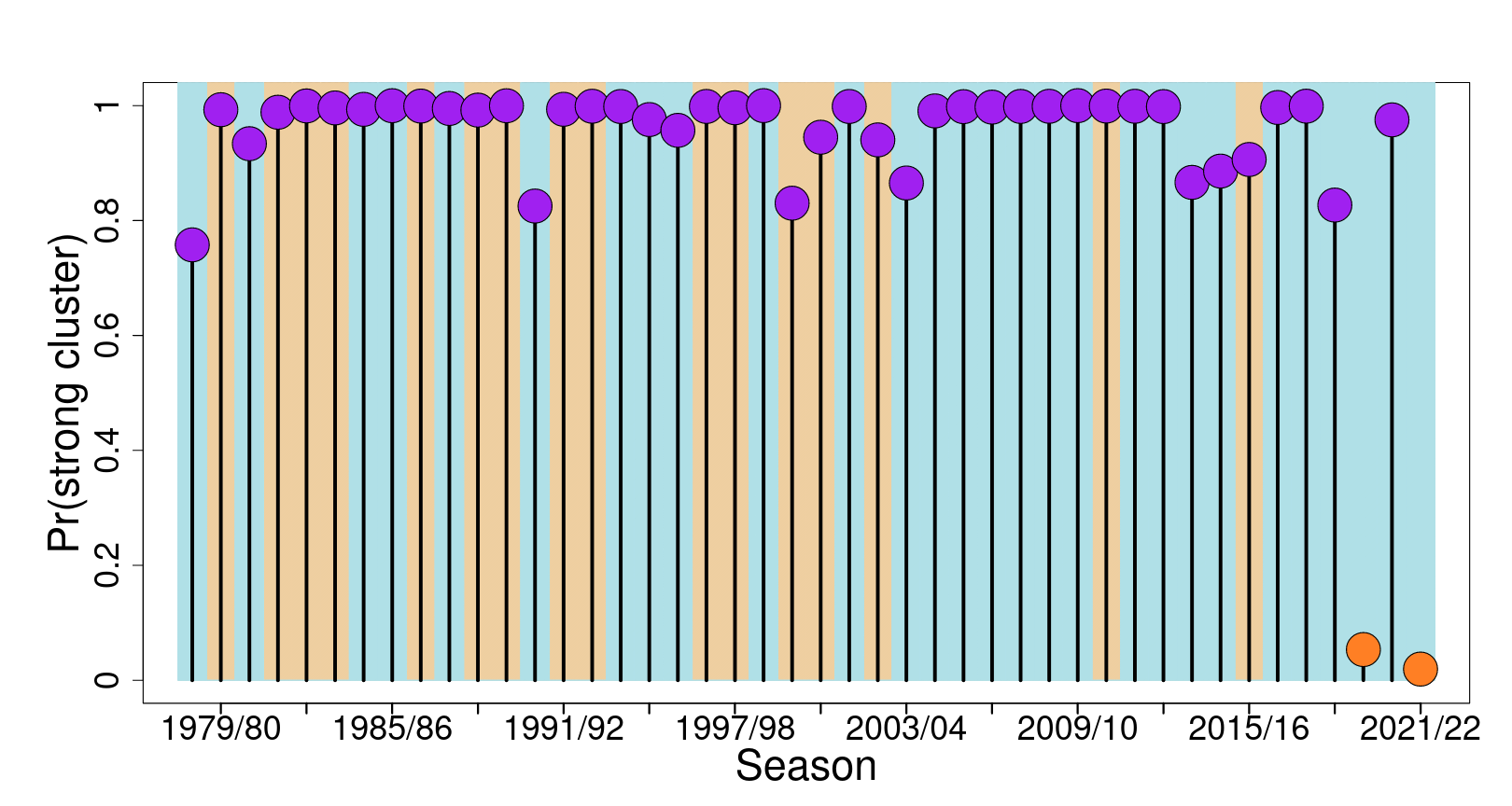
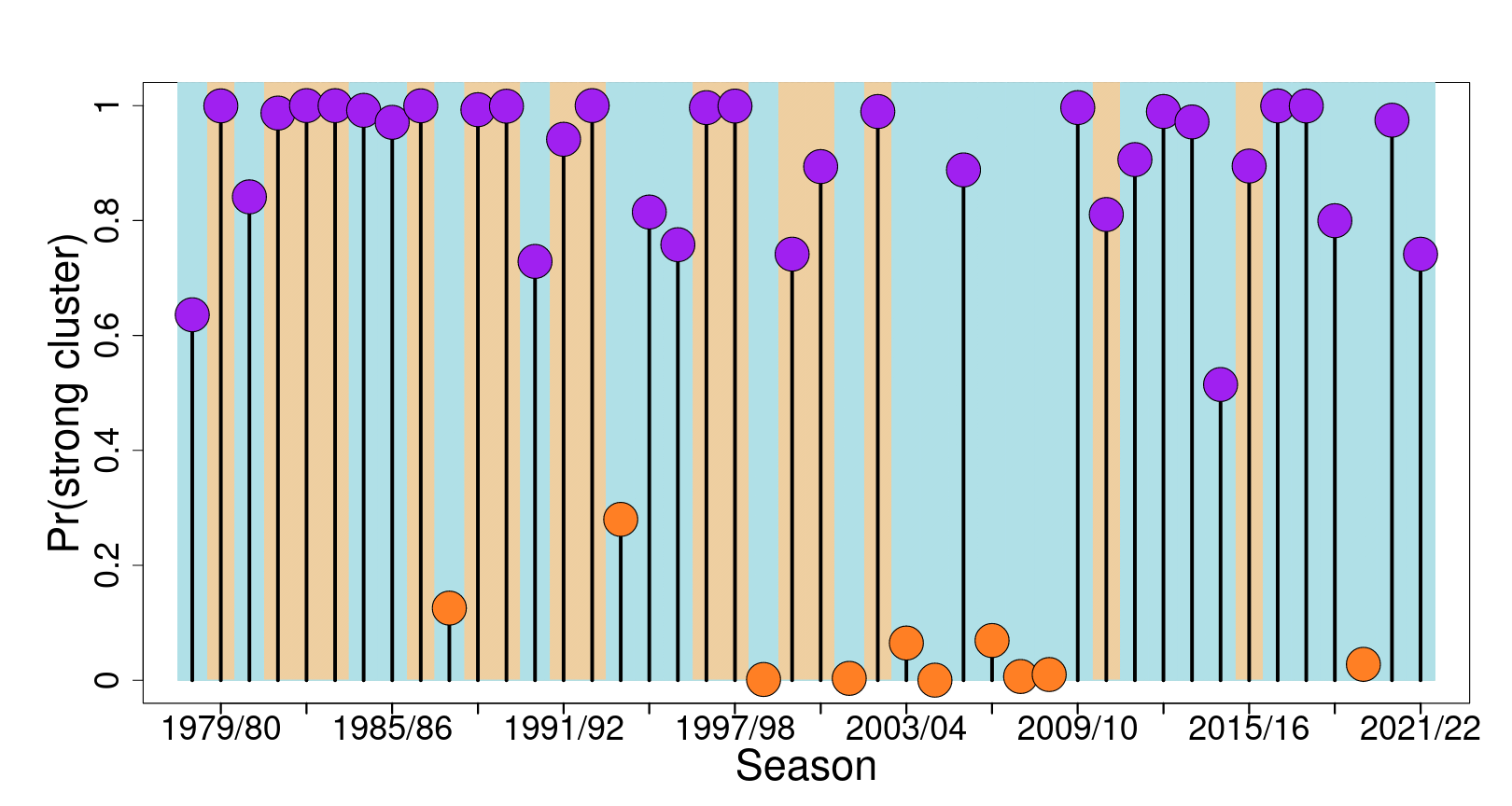
Figure 7: Arsenal.

Figure 8: Chelsea.

Figure 9: Liverpool.

Figure 10: Manchester City.

Figure 11: Manchester United.

Figure 12: Tottenham Hotspur.

Figure 13: Plot of posterior probability of allocation to the strongest block for some selected teams over the entire study period. The x-axis indicates each season in chronological order, while the y-axis displays the posterior probability of inclusion in the strongest block where each team is indicated with a purple dot if its posterior allocation probability is greater than 0.5 or with an orange one otherwise. If no dot is present for any time period it means that team was not playing in the First division/Premier League for that season. The background indicates how many blocks have been chosen with highest posterior probability. In particular, a sand coloured background is used for single-block model and a light blue colour is for a two block model.

6.2.2 Validation of the SBM approach using two standard indices

Here we revisit the statistics outlined in Section 2. We once again display both HHICB and relative entropy for each season. But now, in Figure 14 we overlay the posterior probability of $K=1$ for each season. We see both plots illustrate that, in general, seasons with a lower HHICB score (higher relative entropy, respectively) tend to correspond to seasons where a single block had the most posterior support. Effectively, the HHICB and relative entropy scores are broadly in agreement with the results of our stochastic block model and provide a validation of our SBM approach.

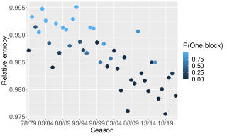
(a)	(b)

Figure 14: (a) The Herfindahl–Hirschman index of competitive balance (HHICB) and (b) the relative entropy are plotted for each season, while the posterior probability of a one block model, $\pi(K=1|\bm{y})$, is overlaid for each season. Both plots illustrates that, in general, seasons with a lower HHICB score (higher relative entropy, respectively) tend to correspond to seasons where a single block had the most posterior support.

6.3 Evidence for the emergence of a big-six groups of teams

In this section we explore if there is some statistical evidence for two well known phenomena in popular discourse: the dominance of the big-four (a group of four teams, namely, Arsenal, Chelsea, Liverpool and Manchester United) during the mid-2000’s and the emergence of a big-six from 2010 with the addition of Manchester City and Tottenham Hotspur. To investigate this, consider Table 4 where we present the posterior allocation of teams to the strongest block of teams for the past two decades from $2003/04$ to $2021/22$ following Section 6.2.1.

From $2002/03$ to $2008/09$:

Analysing Table 4 from $2002/03$ to $2008/09$ indicates that Arsenal, Chelsea and Manchester United were ever present in the top block over this time period, while Liverpool were present in four of these seasons. This gives some credence to the notion of a big-four block of teams during this period.

From $2009/10$ to $2021/22$:

By contrast, season $2009/10$ onwards, signified the emergence of Manchester City and Tottenham Hotspur in the top block. In fact, $2009/10$ is when the former was purchased by the Abu Dhabi United Group. Since then, both teams have consistently been allocated to the top block of teams with the exception of Tottenham Hotspur in $2019/20$. In terms of the period from $2009/10$ to $2021/22$, the collection of teams in the strongest block has been remarkable consistent until $2018/19$. However, over the past three seasons, Arsenal and Manchester United have been absent from the strongest block. While Chelsea have been absent in $2019/20$. This tentatively suggests that Arsenal and Manchester United may no longer be considered to among the strongest block of teams and that there is a re-emergence of a top-four. Of course, more seasons are needed to validate this. Finally, it is worth noting that there are some seasons where some teams appear for a couple of consecutive seasons in the strongest block, for example, Everton from $2007/08$ to $2009/10$ and again from $2012/13$ to $2013/14$. We also remark that $2020/21$ was an exceptional season in the sense that the number of teams in the strongest block contained $15$ teams. This season was, of course, impacted by the COVID-19 pandemic when the majority of matches were played behind closed doors and the fact that the strongest block was so large, may suggest that the absence of crowds had the effect of increasing competitive balance.

	Arsenal	Chelsea	Liverpool	Man City	Man Utd	Tottenham	Additional teams
02/03	✓	✓	✓		✓	✓
03/04	✓	✓	✗	✗	✓	✗
04/05	✓	✓	✗	✗	✓	✗
05/06	✓	✓	✓	✗	✓	✓	Blackburn, Newcastle
06/07	✓	✓	✗	✗	✓	✗
07/08	✓	✓	✓	✗	✓	✗	Everton
08/09	✓	✓	✓	✗	✓	✗	Everton, Aston Villa
09/10	✓	✓	✓	✓	✓	✓	Everton, Aston Villa
10/11	✓	✓	✓	✓	✓	✓
11/12	✓	✓	✗	✓	✓	✓	Newcastle
12/13	✓	✓	✓	✓	✓	✓	Everton
13/14	✓	✓	✓	✓	✓	✓	Everton
14/15	✓	✓	✗	✓	✓	✓
16/17	✓	✓	✓	✓	✓	✓
15/16	✓	✓	✓	✓	✓	✓
17/18	✓	✓	✓	✓	✓	✓
18/19	✓	✓	✓	✓	✓	✓
19/20	✗	✗	✓	✓	✗	✗
20/21	✓	✓	✓	✓	✓	✓	$9$ additional teams
21/22	✗	✓	✓	✓	✗	✓
Total no. of Seasons in
the top block (out of 20)	17/20	19/20	15/20	13/20	17/20	14/20

Table 4: Posterior allocation of teams to the strongest block for each season since $2003/04$. Here the symbols ✓and ✗  denote allocation or not, respectively, to the strongest block. Seasons with the highest probability of a single block model are highlighted in colour. Additional teams which were allocated to the strongest block are also listed per season.

7 Conclusions

In this paper we have developed a stochastic block model to allow a probabilistic assessment of competitive balance in the English football league. The important aspect of this model is that it allows one to assess the likely number of blocks of teams in a league, where a block consists of a number of teams such that the probability mass function of the outcome (a win, draw, or loss) is estimated to be the same for a match involving any two teams in that block. Similarly, a match involving a team from one block playing against any team from another block has its own between-block probability mass function for the outcome of that match. In contrast to previous approaches, our model approach yields a richer understanding of the nature of the competitiveness of a league through estimation of the posterior probability of the number of blocks, together with the most likely allocation of teams to each block. But also it allows one to estimate the number of teams allocated to the strongest block of teams, by integrating over the posterior uncertainty in the number of blocks.

In terms of our analysis of the English Premier League, we have uncovered evidence that the league was quite balanced from around $1980$ to $2003$. However, subsequent to that, there is strong evidence that the league has become more imbalanced since from $2003/04$ we see an emergence of seasons where two blocks are most probable, a posteriori. This is further supported by our analysis which shows that the estimated number of teams in the strongest block of teams is typically quite large from $1980$ to around $2003$, in contrast to the second half of the study period where the number of teams estimated to be in strongest block is, in general, much smaller. Our findings may serve to provide the Premier League with quantitative evidence of a lack of competitiveness over the past two decades which in turn may inform policy around potential reform of the league structure to address this issue. For example, it would be of interest to understand the effect which a more equal redistribution of television revenue may have on competitive balance.

This paper could be extended in several directions. For example, the stochastic block model does not directly model for the number of goals scored by either team. In fact, there is a steady literature on statistical models for football match data beginning with (Dixon and Coles, 1997), where a Poisson GLM framework is used to model the number of goals scored by either team. This has been extended by several authors, including Karlis and Ntzoufras (2003) to the bivariate Poisson setting. While Rue and Salvesen (2000) extend the Dixon and Coles framework to a Bayesian dynamic GLM setting. There would therefore be interest in extending our modified stochastic block model to accommodate models for the number of goals scored by both teams using some of these frameworks. A further extension would be the development of a statistical changepoint model to assess the uncertainty around the season where a changepoint has occured. Finally we note that it would be natural to extend our SBM to incorporate temporal dependence across seasons.

Datasets and code

All of the datasets and R code used to reproduce the results and figures in this paper can be found at https://github.com/francescabasini/Football_SBM

Appendix A Calculation of the collapsed SBM

A.1 Collapsing p

$\displaystyle f(\bm{y}|\bm{z},K)$ $\displaystyle=\int_{\bm{p}}f(\bm{y}|\bm{z},\bm{p},K)\pi(\bm{p}|K)d\bm{p}$ $\displaystyle=\int_{p_{\omega}^{kl}\in\underline{p}^{kl}\in\bm{p}}\prod_{i=1}^{N-1}\prod_{\underset{j\neq i}{j=1}}^{N}\prod_{k=1}^{K}\prod_{l=1}^{K}\left(\prod_{\omega=1}^{3}\left(p_{\omega}^{kl}\right)^{I(y_{ij}=\omega)}\right)^{I\left(z_{i}=k\right)I\left(z_{j}=l\right)}\cdot\prod_{k=1}^{K}\prod_{l=1}^{K}\frac{1}{B(\bm{\beta})}\prod_{\omega=1}^{3}\left(p_{\omega}^{kl}\right)^{\beta_{\omega}-1}dp_{\omega}^{kl}$ $\displaystyle\begin{aligned} =\int_{p_{\omega}^{kl}\in\underline{p}^{kl}\in\bm{p}}\prod_{k=1}^{K}\prod_{l=1}^{K}\prod_{\omega=1}^{3}\left(p_{\omega}^{kl}\right)^{\sum_{i=1}^{N-1}\sum_{\underset{j\neq i}{j=1}}^{N}I(y_{ij}=\omega){I\left(z_{i}=k\right)I\left(z_{j}=l\right)}}\prod_{k=1}^{K}\prod_{l=1}^{K}\frac{1}{B(\bm{\beta})}\prod_{\omega=1}^{3}\left(p_{\omega}^{kl}\right)^{\beta_{\omega}-1}dp_{\omega}^{kl}\end{aligned}$ (18)

Here we define

$$N_{kl}^{\omega}=\sum_{i=1}^{N-1}\sum_{\underset{j\neq i}{j=1}}^{N}{I(y_{ij}=\omega)I\left(z_{i}=k\right)I\left(z_{j}=l\right)},$$ (19)

for $k=1,\dots,K$ and $l=1,\dots,K$, so that $N_{kl}^{\omega}$ counts the number of times that the outcome $\omega$ was observed for all games involving a team allocated to block $k$ playing at home against a team allocated to block $l$. Thus, we can rewrite (18) as:

$$f(\bm{y}|\bm{z},K) =\int_{p_{\omega}^{kl}\in\underline{p}^{kl}\in\bm{p}}\prod_{k=1}^{K}\prod_{l=1}^{K}\prod_{\omega=1}^{3}\left(p_{\omega}^{kl}\right)^{N_{kl}^{\omega}}\cdot\prod_{k=1}^{K}\prod_{l=1}^{K}\frac{1}{B(\bm{\beta})}\prod_{\omega=1}^{3}\left(p_{\omega}^{kl}\right)^{\beta_{\omega}-1}dp_{\omega}^{kl}.$$

$$= \prod_{k=1}^{K}\prod_{l=1}^{K}\frac{1}{B(\bm{\beta})}\int_{p_{\omega}^{kl}\in\underline{p}^{kl}\in\bm{p}}\prod_{\omega=1}^{3}\left(p_{\omega}^{kl}\right)^{N_{kl}^{\omega}+\beta_{\omega}-1}dp_{\omega}^{kl},$$ (20)

Inside (20), we recognise the kernel of a 3-dimensional Dirichlet distribution of the form:

$$(p_{1}^{kl},p_{2}^{kl},p_{3}^{kl})\sim Dir(N_{kl}^{\omega=1}+\beta_{1},N_{kl}^{\omega=2}+\beta_{2},N_{kl}^{\omega=3}+\beta_{3}).$$

Therefore, we can re-write the right hand side of equation (20) as:

$$\prod_{k=1}^{K}\prod_{l=1}^{K}\frac{1}{B(\bm{\beta})}\frac{\prod_{\omega=1}^{3}\Gamma(N_{kl}^{\omega}+\beta_{\omega})}{\Gamma(\sum_{\omega=1}^{3}\left(N_{kl}^{\omega}+\beta_{\omega})\right)},$$

where

$$\frac{1}{B(\bm{\beta})}=\frac{\Gamma(\sum_{\omega=1}^{3}\beta_{\omega})}{\prod_{\omega=1}^{3}\Gamma(\beta_{\omega})}.$$

This yields the expression

$$f(\bm{y}|\bm{z},K)=\prod_{k=1}^{K}\prod_{l=1}^{K}\frac{\Gamma(\sum_{\omega=1}^{3}\beta_{\omega})}{\prod_{\omega=1}^{3}\Gamma(\beta_{\omega})}\frac{\prod_{\omega=1}^{3}\Gamma(N_{kl}^{\omega}+\beta_{\omega})}{\Gamma(\sum_{\omega=1}^{3}\left(N_{kl}^{\omega}+\beta_{\omega})\right)}.$$

Recall that in our framework the concentration parameters of the prior Dirichlet distribution of $\underline{p}^{kl}\text{ for }k,l=1,\ldots,K$ are all set to be equal to have a uniform prior,

$$\beta_{\omega}=1,\;\;\mbox{for}\;\;\ \omega=1,2,3\ ,$$

resulting in,

$$f(\bm{y}|\bm{z},K)=\prod_{k=1}^{K}\prod_{l=1}^{K}\Gamma(3)\frac{\prod_{\omega=1}^{3}\Gamma(N_{kl}^{\omega}+1)}{\Gamma(\sum_{\omega=1}^{3}\left(N_{kl}^{\omega}+1)\right)}.$$ (21)

A.2 Collapsing theta

$$\pi(\bm{z}|K) =\int_{\bm{\Theta}}\pi(\bm{z}|\bm{\theta},K)\pi(\bm{\theta}|K)d\bm{\Theta}$$

$$=\int_{\bm{\Theta}}\prod_{i=1}^{N}Multi(z_{i};1,\bm{\theta})\cdot Dir(\bm{\theta};\bm{\gamma})d\bm{\Theta}$$

$$=\int_{\bm{\Theta}}\prod_{i=1}^{N}\prod_{k=1}^{K}\theta_{k}^{I\left(z_{i}=k\right)}\cdot\frac{\Gamma(\sum_{k=1}^{K}\gamma_{k})}{\prod_{k=1}^{K}\Gamma\left(\gamma_{k}\right)}\prod_{k=1}^{K}\theta_{k}^{\gamma_{k}-1}d\bm{\Theta}$$

$$=\Gamma(\sum_{k=1}^{K}\gamma_{k})\int_{\bm{\Theta}}\prod_{k=1}^{K}\theta_{k}^{\sum_{i=1}^{N}I\left(z_{i}=k\right)}\frac{1}{\prod_{k=1}^{K}\Gamma(\gamma_{k})}\prod_{k=1}^{K}\theta_{k}^{\gamma_{k}-1}d\bm{\Theta}$$

$$=\Gamma(\sum_{k=1}^{K}\gamma_{k})\int_{\bm{\Theta}}\prod_{k=1}^{K}\theta_{k}^{\sum_{i=1}^{N}I\left(z_{i}=k\right)+\gamma_{k}-1}\frac{1}{\Gamma(\gamma_{k})}d\bm{\Theta}$$ (22)

We set

$$n_{k}=\sum_{i=1}^{N}{I\left(z_{i}=k\right)},\ k=1,\ldots,K,$$ (23)

where each $n_{k}$ accounts for the number of nodes/teams allocated to block $k$. Therefore we can rewrite the right hand side of (22) as:

$$\Gamma(\sum_{k=1}^{K}\gamma_{k})\int_{\bm{\Theta}}\prod_{k=1}^{K}\theta_{k}^{n_{k}+\gamma_{k}-1}\frac{1}{\Gamma(\gamma_{k})}d\bm{\Theta}$$

$$=\frac{\Gamma(K\cdot\gamma_{0})}{\prod_{k=1}\Gamma(\gamma_{0})}\int_{\bm{\Theta}}\prod_{k=1}^{K}\theta_{k}^{n_{k}+\gamma_{0}-1}d\bm{\Theta}\ .$$

We recognise the integral above as the density of a $Dir(n_{1}+\gamma_{0},\ldots,n_{K}+\gamma_{0})$ distribution, thus we can write:

$$\pi(\bm{z}|K) =\frac{\Gamma(K\cdot\gamma_{0})}{\prod_{k=1}^{K}\Gamma(\gamma_{0})}\frac{\prod_{k=1}^{K}\Gamma(n_{k}+\gamma_{0})}{\Gamma(\sum_{k=1}^{K}(n_{k}+\gamma_{0}))}$$

$$=\frac{\prod_{k=1}^{K}\Gamma(n_{k}+\gamma_{0})}{\Gamma^{K}(\gamma_{0})}\frac{\Gamma(K\cdot\gamma_{0})}{\Gamma(N+K\gamma_{0})}\ .$$

Setting the hyperparameter $\gamma_{0}=1$, leads to

$$\pi(\bm{z}|K)=\prod_{k=1}^{K}\Gamma(n_{k}+1)\frac{\Gamma(K)}{\Gamma(N+K)}.$$ (24)

Collapsed posterior

Using (21) and (24) results in the expression for the collapsed posterior,

$$\pi(\bm{z}|\bm{y},K) \propto f(\bm{y}|\bm{z},K)\pi(\bm{z}|K)\pi(k)$$

$$=\prod_{k=1}^{K}\prod_{l=1}^{K}\Gamma(3)\frac{\prod_{\omega=1}^{3}\Gamma(N_{kl}^{\omega}+1)}{\Gamma(\sum_{\omega=1}^{3}\left(N_{kl}^{\omega}+1)\right)}\cdot\prod_{k=1}^{K}\Gamma(n_{k}+1)\frac{\Gamma(K)}{\Gamma(N+K)}\times\frac{1}{K!}\,.$$ (25)

.

Appendix B Details of the MCMC move types

B.1 Acceptance probabilities of the MK move

Insert attempt

The proposal probabilities formulated in terms of an insert attempt are:

$$P_{prop}((\bm{z},K)\rightarrow(\bm{z}^{\prime},K^{\prime})) =P_{prop}((\bm{z},K)\rightarrow(\bm{z},K+1))$$

$$=Pr(\text{Insert an empty cluster})$$

$$=\begin{cases}0.5,\ \text{if }K<K_{max}\\ 0,\text{ if }K=K_{max}.\end{cases}$$

$$P_{prop}((\bm{z}^{\prime},K^{\prime})\rightarrow(\bm{z},K)) =P_{prop}((\bm{z},K+1)\rightarrow(\bm{z},K))$$

$$=Pr(\text{Delete an empty cluster})$$

$$=0.5$$

Recall that the algorithm will reject the move to increase the number of clusters when $K=K_{max}$ and also that this move does not propose to change $\bm{z}$. Here, when $K<K_{max}$ the ratio of the posterior density at the proposed and current states can be written as:

$$\frac{\pi(\bm{z},K^{\prime}|\bm{y})}{\pi(\bm{z},K|\bm{y})} =\frac{f(\bm{y}|\bm{z})\pi(\bm{z}|K^{\prime})\pi(K^{\prime})}{f(\bm{y}|\bm{z})\pi(\bm{z}|K)\pi(K)}$$

$$=\frac{\pi(\bm{z}|K+1)}{\pi(\bm{z}|K)}\times\frac{\pi(K+1)}{\pi(K)}$$

$$=\frac{\left(\prod_{k=1}^{K+1}\Gamma(n_{k}+1)\frac{\Gamma((K+1))}{\Gamma(N+(K+1))}\right)}{\left(\prod_{k=1}^{K}\Gamma(n_{k}+1)\frac{\Gamma(K)}{\Gamma(N+K)}\right)}\times\frac{K!}{(K+1)!}\ .$$ (26)

Note that since the newly inserted cluster is not allocated any nodes,

$$\prod_{k=1}^{K+1}\Gamma(n_{k}+1)=\prod_{k=1}^{K}\Gamma(n_{k}+1)$$

and so (26) reduces to

$$\frac{\pi(\bm{z},K^{\prime}|\bm{y})}{\pi(\bm{z},K|\bm{y})} =\frac{\left(\frac{\Gamma((K+1)}{\Gamma(N+(K+1)}\right)}{\left(\frac{\Gamma(K)}{\Gamma(N+K)}\right)}\times\frac{1}{K+1}$$

$$=\frac{K}{(N+K)(K+1)}.$$ (27)

Since we have symmetric proposal probabilities when $K<K_{max}$, the acceptance probability of the insert attempt is:

$$\alpha=\frac{K}{(N+K)(K+1)}$$ (28)

Delete attempt

For the delete attempt, provided that $K>1$, the proposal probabilities are:

$$P_{prop}((\bm{z},K)\rightarrow(\bm{z}^{\prime},K^{\prime})) =P_{prop}((\bm{z},K)\rightarrow(\bm{z},K-1))$$

$$=Pr(\text{delete an empty cluster})$$

$$=\begin{cases}0.5,\ \text{if }K>1\\ 0,\text{ if }K=1.\end{cases}$$

$$P_{prop}((\bm{z}^{\prime},K^{\prime})\rightarrow(\bm{z},K)) =P_{prop}((\bm{z},K-1)\rightarrow(\bm{z},K))$$

$$=Pr(\text{Insert an empty cluster})$$

$$=0.5$$

Notice again that, due to the way the algorithm is built, we will prevent a delete move from taking place if $K=1$. Here, when $K>1$ the ratio of the posterior density at the proposed and current states can be written as:

$$\frac{\pi(\bm{z},K^{\prime}|\bm{y})}{\pi(\bm{z},K|\bm{y})} =\frac{f(\bm{y}|\bm{z})\pi(\bm{z}|K^{\prime})\pi(K^{\prime})}{f(\bm{y}|\bm{z})\pi(\bm{z}|K)\pi(K)}$$

$$=\frac{\pi(\bm{z}|K-1)}{\pi(\bm{z}|K)}\times\frac{\pi(K-1)}{\pi(K)}$$

$$=\frac{\left(\prod_{k=1}^{K-1}\Gamma(n_{k}+1)\frac{\Gamma((K-1))}{\Gamma(N+(K-1))}\right)}{\left(\prod_{k=1}^{K}\Gamma(n_{k}+1)\frac{\Gamma(K)}{\Gamma(N+K}\right)}\times\frac{K!}{(K-1)!}\ .$$ (29)

Since a delete move involves removing an empty cluster,

$$\prod_{k=1}^{K-1}\Gamma(n_{k}+1)=\prod_{k=1}^{K}\Gamma(n_{k}+1)$$

and so (29) reduces to

$$\frac{\pi(\bm{z},K^{\prime}|\bm{y})}{\pi(\bm{z},K|\bm{y})}=\frac{K(N+K-1)}{K-1}\,.$$

The acceptance probability of delete attempt when $K>1$, since this results in symmetric proposal probabilities, is:

$$\alpha=\frac{K(N+K-1)}{K-1}.$$ (30)

B.2 Acceptance probability for Metropolis-within-Gibbs move

Here we provide some details on the acceptance probability outlined in equation (11) in the manuscript. We can express this as

$$\frac{\pi(\bm{z}^{\prime},K|\bm{y})}{\pi(\bm{z}^{(s+1)},K|\bm{y})}=\frac{\prod_{k=1}^{K}\prod_{l=1}^{K}\frac{\prod_{\omega=1}^{3}\Gamma(N_{kl}^{\omega^{\prime}}+1)}{\Gamma(\sum_{\omega=1}^{3}\left(N_{kl}^{\omega^{\prime}}+1)\right)}}{\prod_{k=1}^{K}\prod_{l=1}^{K}\frac{\prod_{\omega=1}^{3}\Gamma(N_{kl}^{\omega}+1)}{\Gamma(\sum_{\omega=1}^{3}\left(N_{kl}^{\omega}+1)\right)}}\times\frac{\prod_{k=1}^{K}\Gamma(n_{k}^{{}^{\prime}}+1)}{\prod_{k=1}^{K}\Gamma(n_{k}^{{}^{\prime}}+1)},$$ (31)

where $N_{kl}^{\omega^{\prime}}$ is the equivalent quantity calculated in (19), but applied to the proposed allocation vector $\bm{z}^{\prime}$,

$$N_{kl}^{\omega^{\prime}}=\sum_{i=1}^{N-1}\sum_{\underset{j\neq i}{j=1}}^{N}{I(y_{ij}=\omega)I\left(z_{i}^{{}^{\prime}}=k\right)I\left(z_{j}^{{}^{\prime}}=l\right)}.$$

However, recall that proposed allocation vector $\bf{z}^{\prime}$ is identical to the current state of the allocation vector, $\bm{z}^{(s+1)}$, except for its $i$th element, $z_{i}^{\prime}$, which we suppose is allocated the label $k_{1}$. Further, suppose that the current state $z_{i}^{(s+1)}=k_{0}$. It turns out that this leads to some simplification in the first term in the right hand side of (31), since in this case,

$$N_{kl}^{\omega^{\prime}}=\begin{cases}N_{kl}^{\omega^{\prime}},\text{ if }k=k_{0}\ or\ k=k_{1}\ or\ l=k_{1}\ or\ l=k_{0},\\ N_{kl}^{\omega}\ ,\ \text{otherwise.}\end{cases}$$ (32)

This leads to a significant saving in the calculation of this term in (31). The second term on the right hand side of (31) can also be simplified. Since in this case, we note that $n_{k}^{{}^{\prime}}$ is defined similar to (23) as

$$n_{k}^{{}^{\prime}}=\sum_{i=1}^{N}{I\left(z_{i}^{{}^{\prime}}=k\right)},\ k=1,\ldots,K,$$ (33)

and again we remark that $\bm{z}^{\prime}$ is identical to the current state of the allocation vector, $\bm{z}^{(s+1)}$, except for its $i$th element, $z_{i}^{\prime}=k_{1}$. This implies that

$$n_{k}^{{}^{\prime}}=\begin{cases}n_{k_{1}}+1,\text{ if }k=k_{1},\\ n_{k_{0}}-1,\text{ if }k=k_{0},\\ n_{k}\ ,\ \text{otherwise.}\end{cases}$$ (34)

consequently, the second term on the right hand side of (31) can be written as

$$\frac{\prod_{k=1}^{K}\Gamma(n^{\prime}_{k}+1)}{\prod_{k=1}^{K}\Gamma(n_{k}+1)} =\frac{\Gamma(n_{k_{0}})\Gamma(n_{k_{1}}+2)}{\Gamma(n_{k_{1}}+1)\Gamma(n_{k_{0}}+1)}$$

$$=\frac{n_{k_{1}}+1}{n_{k_{0}}}\ .$$ (35)

B.3 Acceptance probabilities of the AE move

B.3.1 Ejection attempt

The proposal probabilities of an ejection attempt can be written as:

$$P_{prop}((\bm{z}^{\prime},K^{\prime})\rightarrow(\bm{z},K)) =P_{prop}((\bm{z}^{\prime},K+1)\rightarrow(\bm{z},K))$$

$$=Pr(\text{absorb a cluster})\times\frac{1}{\begin{subarray}{c}\text{ \# labels for}\\ \text{absorbing cluster}\end{subarray}}\times\frac{1}{\begin{subarray}{c}\text{ \# labels for}\\ \text{absorbed cluster}\end{subarray}}$$

$$=(1-p_{K}^{e})\frac{1}{K+1}\frac{1}{K}.$$

While the reverse proposal probability is detailed as:

$$P_{prop}((\bm{z},K)\rightarrow(\bm{z}^{\prime},K^{\prime})) =P_{prop}((\bm{z},K)\rightarrow(\bm{z}^{\prime},K+1))$$

$$=Pr(\text{eject a cluster})\times\frac{1}{\begin{subarray}{c}\text{ \# labels for}\\ \text{ ejecting cluster}\end{subarray}}\times\frac{1}{\begin{subarray}{c}\text{\# labels for}\\ \text{ejected cluster}\end{subarray}}\times Pr(\text{new allocation for }\bm{z})$$

$$=p_{K}^{e}\times\frac{1}{K+1}\times\frac{1}{K}\times\binom{n_{j_{1}}+n_{j_{2}}}{n_{j_{1}}}p_{E}^{n_{j_{2}}}(1-p_{E})^{n_{j_{1}}}\cdot\frac{p_{E}^{a-1}(1-p_{E})^{a-1}}{B(a,a)}$$ (36)

for $p_{E}\sim Beta(a,a)$ and where,

$$n_{j_{1}} =\sum_{i=1}^{N}I(z^{\prime}_{i}=j_{1})\text{ is the number of nodes in the ejecting cluster after reallocation,}$$

$$n_{j_{2}} =\sum_{i=1}^{N}I(z^{\prime}_{i}=j_{2})\text{ is the number of nodes in the ejected cluster.}$$

After integrating out with respect to the distribution of $p_{E}$, the resulting proposal probability in (36) reduces to:

$$p_{K}^{e}\times\frac{1}{K+1}\times\frac{1}{K}\times\binom{n_{j_{1}}+n_{j_{2}}}{n_{j_{1}}}\frac{1}{B(a,a)}\int_{0}^{1}p_{E}^{n_{j_{2}}+a-1}(1-p_{E})^{n_{j_{1}}+a-1}dp_{E}$$

$$=p_{K}^{e}\times\frac{1}{K+1}\times\frac{1}{K}\times\frac{(n_{j_{1}}+n_{j_{2}})!}{n_{j_{1}}!n_{j_{2}}!}\frac{\Gamma(2a)}{\Gamma(a)\Gamma(a)}\frac{\Gamma(n_{j_{1}}+a)\Gamma(n_{j_{2}}+a)}{\Gamma(n_{j_{1}}+n_{j_{2}}+2a)}$$

$$=p_{K}^{e}\times\frac{1}{K+1}\times\frac{1}{K}\times\frac{1}{n_{j_{1}}+n_{j_{2}}+1}.$$

The final equation above follows from setting $a=1$, so that $p_{E}\sim U(0,1)$, as in McDaid et al. (2013).

The posterior probability ratio for the ejection attempt takes the following form:

$$\frac{\pi(\bm{z}^{\prime},K^{\prime}|Y)}{\pi(\bm{z},K|Y)} =\frac{f(Y|\bm{z}^{\prime})\pi(\bm{z}^{\prime}|K^{\prime})\pi(K^{\prime})}{f(Y|\bm{z})\pi(\bm{z}|K)\pi(K)}$$

$$=\frac{f(Y|\bm{z}^{\prime})\pi(\bm{z}^{\prime}|K+1)\pi(K+1)}{f(Y|\bm{z})\pi(\bm{z}|K)\pi(K)}$$

$$=\frac{\prod_{k=1}^{K+1}\prod_{l=1}^{K+1}\frac{\prod_{\omega=1}^{3}\Gamma(N_{kl}^{\omega^{\prime}}+1)}{\Gamma(\sum_{\omega=1}^{3}\left(N_{kl}^{\omega^{\prime}}+1)\right)}}{\prod_{k=1}^{K}\prod_{l=1}^{K}\frac{\prod_{\omega=1}^{3}\Gamma(N_{kl}^{\omega}+1)}{\Gamma(\sum_{\omega=1}^{3}\left(N_{kl}^{\omega}+1)\right)}}\times\frac{\prod_{k=1}^{K+1}\Gamma(n_{k}^{{}^{\prime}}+1)\frac{\Gamma(K+1)}{\Gamma(N+K+1)}}{\prod_{k=1}^{K}\Gamma(n_{k}+1)\frac{\Gamma(K)}{\Gamma(N+K)}}\times\frac{K!}{(K+1)!}$$

$$=\frac{\prod_{k=1}^{K+1}\prod_{l=1}^{K+1}\frac{\prod_{\omega=1}^{3}\Gamma(N_{kl}^{\omega^{\prime}}+1)}{\Gamma(\sum_{\omega=1}^{3}\left(N_{kl}^{\omega^{\prime}}+1)\right)}}{\prod_{k=1}^{K}\prod_{l=1}^{K}\frac{\prod_{\omega=1}^{3}\Gamma(N_{kl}^{\omega}+1)}{\Gamma(\sum_{\omega=1}^{3}\left(N_{kl}^{\omega}+1)\right)}}\times\frac{\prod_{k=1}^{K+1}\Gamma(n_{k}^{{}^{\prime}}+1)}{\prod_{k=1}^{K}\Gamma(n_{k}+1)}\times\frac{K}{(N+K)(K+1)}$$

B.3.2 Absorption attempt

The proposal probabilities of the absorption move are:

$$P_{prop}((\bm{z}^{\prime},K^{\prime})\rightarrow(\bm{z},K)) =P_{prop}((\bm{z}^{\prime},K-1)\rightarrow(\bm{z},K))$$

$$=Pr(\text{absorb a cluster})\times\frac{1}{\begin{subarray}{c}\text{ \# labels for}\\ \text{absorbing cluster}\end{subarray}}\times\frac{1}{\begin{subarray}{c}\text{ \# labels for}\\ \text{absorbed cluster}\end{subarray}}$$

$$=(1-p_{K}^{e})\frac{1}{K-1}\frac{1}{K}.$$

$$P_{prop}((\bm{z},K)\rightarrow(\bm{z}^{\prime},K^{\prime})) =P_{prop}((\bm{z},K)\rightarrow(\bm{z}^{\prime},K+1))$$

$$=Pr(\text{eject a cluster})\times\frac{1}{\begin{subarray}{c}\text{ \# labels for}\\ \text{ ejecting cluster}\end{subarray}}\times\frac{1}{\begin{subarray}{c}\text{\# labels for}\\ \text{ejected cluster}\end{subarray}}\times Pr(\text{new allocation for }\bm{z})$$

$$=p_{K}^{e}\times\frac{1}{K-1}\times\frac{1}{K}\times\binom{n_{j_{1}}+n_{j_{2}}}{n_{j_{1}}}p_{E}^{n_{j_{2}}}(1-p_{E})^{n_{j_{1}}}\cdot\frac{p_{E}^{a-1}(a-p_{E})^{a-1}}{B(a,a)}$$

$$=p_{K}^{e}\times\frac{1}{K-1}\times\frac{1}{K}\times\frac{1}{n_{j_{1}}+n_{j_{2}}+1}\,.$$

Where, as before, the final equation above results from setting $a=1$. The posterior probability ratio is given by:

$$\frac{\pi(\bm{z}^{\prime},K^{\prime}|Y)}{\pi(\bm{z},K|Y)} =\frac{f(Y|\bm{z}^{\prime})\pi(\bm{z}^{\prime}|K^{\prime})\pi(K^{\prime})}{f(Y|\bm{z})\pi(\bm{z}|K)\pi(K)}$$

$$=\frac{f(Y|\bm{z}^{\prime})\pi(\bm{z}^{\prime}|K-1)\pi(K-1)}{f(Y|\bm{z})\pi(\bm{z}|K)\pi(K)}$$

$$=\frac{\prod_{k=1}^{K-1}\prod_{l=1}^{K-1}\frac{\prod_{\omega=1}^{3}\Gamma(N_{kl}^{\omega^{\prime}}+1)}{\Gamma(\sum_{\omega=1}^{3}\left(N_{kl}^{\omega^{\prime}}+1)\right)}}{\prod_{k=1}^{K}\prod_{l=1}^{K}\frac{\prod_{\omega=1}^{3}\Gamma(N_{kl}^{\omega}+1)}{\Gamma(\sum_{\omega=1}^{3}\left(N_{kl}^{\omega}+1)\right)}}\times\frac{\prod_{k=1}^{K-1}\Gamma(n_{k}^{{}^{\prime}}+1)\frac{\Gamma(K-1)}{\Gamma(N+K-1)}}{\prod_{k=1}^{K}\Gamma(n_{k}+1)\frac{\Gamma(K)}{\Gamma(N+K)}}\times\frac{K!}{(K-1)!}$$

$$=\frac{\prod_{k=1}^{K+1}\prod_{l=1}^{K+1}\frac{\prod_{\omega=1}^{3}\Gamma(N_{kl}^{\omega^{\prime}}+1)}{\Gamma(\sum_{\omega=1}^{3}\left(N_{kl}^{\omega^{\prime}}+1)\right)}}{\prod_{k=1}^{K}\prod_{l=1}^{K}\frac{\prod_{\omega=1}^{3}\Gamma(N_{kl}^{\omega}+1)}{\Gamma(\sum_{\omega=1}^{3}\left(N_{kl}^{\omega}+1)\right)}}\times\frac{\prod_{k=1}^{K-1}\Gamma(n_{k}^{{}^{\prime}}+1)}{\prod_{k=1}^{K}\Gamma(n_{k}+1)}\times\frac{K(N+K-1)}{K-1}$$

Appendix C Additional results for season $2021/22$

We reproduce the table from Table 1 in the manuscript presenting $\pi(K|\bm{y})$ for $K=1,2,3$. Here we have omitted $\pi(K=4|\bm{y})$ as this had an estimated probability of $3\times 10^{-4}$.

$K$	1	2	3
$\pi(K|\bm{y})$	$0.0$	$0.97$	$0.03$

Table 5: Posterior probabilities for values of $K$

Table 6: Model $K=2$: Posterior allocation probability (as a percentage) for each team

	ARS	AVL	BRE	BHA	BUR	CHE	CRY	EVE	LEE	LEI
Cluster 1	38.29	0.00	0.02	0.50	0.00	89.11	0.03	0.00	0.00	0.15
Cluster 2	61.71	100.00	99.98	99.50	100.00	10.89	99.97	100.00	100.00	99.85
	LIV	MCI	MUN	NEW	NOR	SOU	TOT	WAT	WHU	WOL
Cluster 1	100.00	100.00	1.95	0.04	0.00	0.01	74.75	0.00	0.86	0.53
Cluster 2	0.00	0.00	98.05	99.96	100.00	99.99	25.25	100.00	99.14	99.47

Table 7: Model $K=3$: Posterior allocation probability (as a percentage) for each team

	ARS	AVL	BRE	BHA	BUR	CHE	CRY	EVE	LEE	LEI
Cluster 1	27.52	0.27	0.80	1.25	0.00	60.68	0.01	0.00	0.00	0.36
Cluster 2	16.28	0.57	1.51	4.99	0.37	18.86	1.22	1.27	0.60	0.48
Cluster 3	56.21	99.17	97.69	93.75	99.63	20.47	98.76	98.73	99.40	99.17
	LIV	MCI	MUN	NEW	NOR	SOU	TOT	WAT	WHU	WOL
Cluster 1	64.54	95.47	0.52	0.33	0.00	0.12	56.80	0.00	1.19	0.61
Cluster 2	35.46	4.53	1.30	0.39	4.23	0.66	36.40	5.22	3.99	1.04
Cluster 3	0.00	0.00	98.18	99.28	95.77	99.22	6.80	94.78	94.81	98.35

Appendix D Comparison using a Uniform prior for K

D.1 Details of the MCMC move type when using a Uniform prior for K

Uniform prior for $K$:

We choose a discrete uniform prior for $K$ between 1 and $K_{max}$, where $K_{max}$ is again a user specified upper limit on the plausible number of blocks,

$$K\sim U(1,K_{max})\,.$$

The choice of a different prior leads to the follwing changes for the acceptante probabilities:

D.1.1 Acceptance probabilities of the MK move

Insert attempt

Under the uniform prior, all states of $K$ have the same probability thus the ratio of the posterior density at the proposed and current states can be simplified as:

$$\frac{\pi(\bm{z},K^{\prime}|\bm{y})}{\pi(\bm{z},K|\bm{y})} =\frac{f(\bm{y}|\bm{z})\pi(\bm{z}|K^{\prime})}{f(\bm{y}|\bm{z})\pi(\bm{z}|K)}$$

$$=\frac{\pi(\bm{z}|K+1)}{\pi(\bm{z}|K)}$$

$$=\frac{\prod_{k=1}^{K+1}\Gamma(n_{k}+1)\frac{\Gamma((K+1))}{\Gamma(N+(K+1))}}{\prod_{k=1}^{K}\Gamma(n_{k}+1)\frac{\Gamma(K)}{\Gamma(N+K)}}\ .$$ (37)

Hence, similarly to (27), (37) reduces to:

$$\frac{\pi(\bm{z},K^{\prime}|\bm{y})}{\pi(\bm{z},K|\bm{y})} =\frac{\frac{\Gamma((K+1)}{\Gamma(N+(K+1)}}{\frac{\Gamma(K)}{\Gamma(N+K)}}$$

$$=\frac{K}{N+K}.$$ (38)

Finally, since we have symmetric proposal probabilities for $K<K_{max}$, the acceptance probability of the insert attempt is:

$$\alpha=\frac{K}{N+K}$$ (39)

Delete attempt

In an analous way, the probability ratio of the probability density at the proposed and current states under a uniform prior for $K$ is:

$$\frac{\pi(\bm{z},K^{\prime}|\bm{y})}{\pi(\bm{z},K|\bm{y})} =\frac{f(\bm{y}|\bm{z})\pi(\bm{z}|K^{\prime})}{f(\bm{y}|\bm{z})\pi(\bm{z}|K)}$$

$$=\frac{\pi(\bm{z}|K-1)}{\pi(\bm{z}|K)}$$

$$=\frac{\prod_{k=1}^{K-1}\Gamma(n_{k}+1)\frac{\Gamma((K-1))}{\Gamma(N+(K-1))}}{\prod_{k=1}^{K}\Gamma(n_{k}+1)\frac{\Gamma(K)}{\Gamma(N+K})}\ .$$ (40)

Using the same argument as for (29), (40) reduces to

$$\frac{\pi(\bm{z},K^{\prime}|\bm{y})}{\pi(\bm{z},K|\bm{y})}=\frac{N+K-1}{K-1}\,.$$

The acceptance probability of delete attempt when $K>1$, since this results in symmetric proposal probabilities, is:

$$\alpha=\frac{N+K-1}{K-1}.$$ (41)

D.1.2 Acceptance probabilities for the Metropolis-within-Gibbs move

This move and thus its associated acceptance probabilities is unchanged under the use of a different prior for $K$.

D.1.3 Acceptance probabilities of the AE move

Ejection attempt

Similar to Appendix D.1.1, the posterior probability ratio for the ejection attempt takes the following form:

$$\frac{\pi(\bm{z}^{\prime},K^{\prime}|Y)}{\pi(\bm{z},K|Y)} =\frac{f(Y|\bm{z}^{\prime})\pi(\bm{z}^{\prime}|K^{\prime})}{f(Y|\bm{z})\pi(\bm{z}|K)}$$

$$=\frac{f(Y|\bm{z}^{\prime})\pi(\bm{z}^{\prime}|K+1)}{f(Y|\bm{z})\pi(\bm{z}|K)}$$

$$=\frac{\prod_{k=1}^{K+1}\prod_{l=1}^{K+1}\frac{\prod_{\omega=1}^{3}\Gamma(N_{kl}^{\omega^{\prime}}+1)}{\Gamma(\sum_{\omega=1}^{3}\left(N_{kl}^{\omega^{\prime}}+1)\right)}}{\prod_{k=1}^{K}\prod_{l=1}^{K}\frac{\prod_{\omega=1}^{3}\Gamma(N_{kl}^{\omega}+1)}{\Gamma(\sum_{\omega=1}^{3}\left(N_{kl}^{\omega}+1)\right)}}\times\frac{\prod_{k=1}^{K+1}\Gamma(n_{k}^{{}^{\prime}}+1)\frac{\Gamma(K+1)}{\Gamma(N+K+1)}}{\prod_{k=1}^{K}\Gamma(n_{k}+1)\frac{\Gamma(K)}{\Gamma(N+K)}}$$

$$=\frac{\prod_{k=1}^{K+1}\prod_{l=1}^{K+1}\frac{\prod_{\omega=1}^{3}\Gamma(N_{kl}^{\omega^{\prime}}+1)}{\Gamma(\sum_{\omega=1}^{3}\left(N_{kl}^{\omega^{\prime}}+1)\right)}}{\prod_{k=1}^{K}\prod_{l=1}^{K}\frac{\prod_{\omega=1}^{3}\Gamma(N_{kl}^{\omega}+1)}{\Gamma(\sum_{\omega=1}^{3}\left(N_{kl}^{\omega}+1)\right)}}\times\frac{\prod_{k=1}^{K+1}\Gamma(n_{k}^{{}^{\prime}}+1)}{\prod_{k=1}^{K}\Gamma(n_{k}+1)}\times\frac{K}{N+K}\,.$$

Absorption attempt

The posterior probability ratio is given by:

$$\frac{\pi(\bm{z}^{\prime},K^{\prime}|Y)}{\pi(\bm{z},K|Y)} =\frac{f(Y|\bm{z}^{\prime})\pi(\bm{z}^{\prime}|K^{\prime})}{f(Y|\bm{z})\pi(\bm{z}|K)}$$

$$=\frac{f(Y|\bm{z}^{\prime})\pi(\bm{z}^{\prime}|K-1)}{f(Y|\bm{z})\pi(\bm{z}|K)}$$

$$=\frac{\prod_{k=1}^{K-1}\prod_{l=1}^{K-1}\frac{\prod_{\omega=1}^{3}\Gamma(N_{kl}^{\omega^{\prime}}+1)}{\Gamma(\sum_{\omega=1}^{3}\left(N_{kl}^{\omega^{\prime}}+1)\right)}}{\prod_{k=1}^{K}\prod_{l=1}^{K}\frac{\prod_{\omega=1}^{3}\Gamma(N_{kl}^{\omega}+1)}{\Gamma(\sum_{\omega=1}^{3}\left(N_{kl}^{\omega}+1)\right)}}\times\frac{\prod_{k=1}^{K-1}\Gamma(n_{k}^{{}^{\prime}}+1)\frac{\Gamma(K-1)}{\Gamma(N+K-1)}}{\prod_{k=1}^{K}\Gamma(n_{k}+1)\frac{\Gamma(K)}{\Gamma(N+K)}}$$

$$=\frac{\prod_{k=1}^{K+1}\prod_{l=1}^{K+1}\frac{\prod_{\omega=1}^{3}\Gamma(N_{kl}^{\omega^{\prime}}+1)}{\Gamma(\sum_{\omega=1}^{3}\left(N_{kl}^{\omega^{\prime}}+1)\right)}}{\prod_{k=1}^{K}\prod_{l=1}^{K}\frac{\prod_{\omega=1}^{3}\Gamma(N_{kl}^{\omega}+1)}{\Gamma(\sum_{\omega=1}^{3}\left(N_{kl}^{\omega}+1)\right)}}\times\frac{\prod_{k=1}^{K-1}\Gamma(n_{k}^{{}^{\prime}}+1)}{\prod_{k=1}^{K}\Gamma(n_{k}+1)}\times\frac{N+K-1}{K-1}\,.$$

D.1.4 Comparison of posterior results

In order to compare the use of a uniform prior for $K$ (where $K_{max}=20$) with respect to the truncated Poisson prior in the paper, we report the most relevant posterior summaries, namely the posterior probability density of $K$ (equivalent to Table 4 in the manuscript) and the barplot displaying the posterior estimate of the number of teams allocated to the strongest block each season (equivalent to Figure 5 in the manuscript).

Number of clusters Season 1 2 3 4 5 78/79 0.44 91.01 8.37 0.18 0.00 79/80 93.73 5.77 0.48 0.02 0.00 80/81 12.85 85.84 1.29 0.02 0.00 81/82 93.65 6.23 0.12 0.00 0.00 82/83 99.56 0.43 0.01 0.00 0.00 83/84 97.82 2.07 0.11 0.00 0.00 84/85 26.39 70.83 2.71 0.07 0.00 85/86 0.04 99.44 0.52 0.00 0.00 86/87 98.92 1.05 0.02 0.00 0.00 87/88 5.84 92.85 1.28 0.03 0.00 88/89 97.99 2.00 0.01 0.00 0.00 89/90 96.40 3.04 0.27 0.27 0.01 90/91 28.68 68.36 2.82 0.13 0.00 91/92 84.32 15.55 0.13 0.00 0.00 92/93 97.38 2.55 0.07 0.00 0.00 93/94 13.75 82.72 3.42 0.10 0.00 94/95 9.96 78.15 11.49 0.40 0.01 95/96 27.60 71.47 0.91 0.02 0.00 96/97 99.17 0.83 0.00 0.00 0.00 97/98 95.60 4.24 0.15 0.01 0.00 98/99 0.03 99.34 0.62 0.01 0.00 99/00 40.73 56.89 2.36 0.02 0.00

Number of clusters Season 1 2 3 4 5 00/01 65.10 26.23 7.41 1.18 0.08 01/02 0.05 98.46 1.46 0.03 0.00 02/03 41.73 55.06 3.08 0.14 0.00 03/04 2.13 82.00 15.38 0.49 0.01 04/05 0.00 99.26 0.74 0.00 0.00 05/06 0.16 91.44 7.61 0.78 0.01 06/07 3.36 88.53 7.92 0.19 0.00 07/08 0.00 78.36 18.88 2.71 0.05 08/09 0.00 96.59 3.30 0.11 0.00 09/10 0.00 81.66 17.59 0.74 0.01 10/11 65.80 33.75 0.43 0.02 0.00 11/12 0.56 94.38 4.99 0.07 0.00 12/13 0.00 98.55 1.44 0.01 0.00 13/14 0.00 96.06 3.86 0.08 0.00 14/15 3.92 83.77 12.03 0.28 0.00 15/16 57.24 41.58 1.14 0.04 0.00 16/17 0.00 96.65 3.29 0.06 0.00 17/18 0.00 92.84 6.88 0.28 0.01 18/19 0.00 92.84 6.92 0.25 0.00 19/20 0.96 94.25 4.73 0.06 0.00 20/21 6.89 84.59 8.13 0.37 0.01 21/22 0.04 88.61 10.85 0.50 0.00

Table 8: Posterior probability of $K$, expressed as a percentage, over the last $44$ seasons, under a uniform prior assumption for $K$. The block model with highest posterior probability is coloured accordingly.

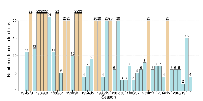
Figure 15: Barplot displaying the posterior estimate of the number of teams allocated to the strongest block each season under a uniform prior assumption for $K$.

The most substantial differences by comparing the posterior results for each season with the two priors are the following:

• Season $1990/91$: For this season, both posterior distributions of $K$ give stronger evidence for $K=2$. However the posterior of allocation of teams $\bm{z}$ in the top block under the uniform prior, integrating over the uncertainty in $K$, places $10$ teams in the strongest block. This constrasts with the corresponding situation for the trunctated Poisson prior where all $20$ teams are placed in the strongest block. However, for the truncated Poisson prior, the posterior probability for $K=2$ is only slighly higher than for $K=1$, which explains the difference in the posterior allocation to the top block after integrating out $K$.

• Season $1993/94$: The uniform prior allocates $4$ teams in the top block instead of $5$ following the truncated Poisson. Note that the posterior probabilities of $K$ under the two priors are in agreement with each other.

• Season $1995/96$: There are $9$ teams in the top block according to the Uniform prior instead of $20$ following the trunctated Poisson prior. A similar comment applies as for Season $1990/91$ above.

• Season $1999/2000$ and $2002/03$: both priors allocate all $20$ teams in the top block but the posterior of $K$ under the Uniform prior gives highest posterior probability to $K=2$, while for the truncated Poisson prior, the highest posterior probability corresponds to $K=1$.

• Season $2014/2015$: There are $4$ teams in the top block instead of $5$ truncated Poisson prior. In both cases, the highest posterior probability for $K$ corresponds to $K=2$.

We can conclude that the Uniform prior generally leads to more blocks, a posteriori, than the truncated Poisson prior, as one would expect. However, despite this, it does not lead to many substantial differences in the posterior allocation of teams to the strongest block, after integrating out the uncertainty in $K$. However, the truncated Poisson prior finds a methodological justification as discussed in Nobile and Fearnside (2005), essentially reflecting the fact that an SBM with $K$ blocks, there are $K!$ permutations of the block labels. For this reason, we restate our preference for the use of a truncated Poisson prior for $K$.

Appendix E Team abbreviations (Season $2021/22$)

ARS	Arsenal
AST	Aston Villa
BRE	Brentford
BHA	Brighton
BUR	Burnley
CHE	Chelsea
CRY	Crystal Palace
EVE	Everton
LEE	Leeds United
LEI	Leicester City
LIV	Liverpool
MCI	Manchester City
MUN	Manchester United
NEW	Newcastle United
NOR	Norwich City
SOU	Southampton
TOT	Tottenham Hotspur
WAT	Watford
WHU	West Ham United
WOL	Wolverhampton Wanderers

References

- Aicher et al. (2015) Aicher, C., A. Z. Jacobs, and A. Clauset (2015). Learning latent block structure in weighted networks. Journal of Complex Networks 3(2), 221–248.
- Biernacki et al. (2000) Biernacki, C., G. Celeux, and G. Govaert (2000). Assessing a mixture model for clustering with the integrated completed likelihood. Pattern Analysis and Machine Intelligence, IEEE Transactions on 22(7), 719–725.
- Borland and MacDonald (2003) Borland, J. and R. MacDonald (2003). Demand for sport. Oxford Review of Economic Policy 19, 478–502.
- Brandes and Franck (2007) Brandes, L. and E. Franck (2007). Who made who? an empirical analysis of competitive balance in European soccer leagues. Eastern Economic Journal 33(3), 379–403.
- Buzzacchi et al. (2003) Buzzacchi, L., S. Szymanski, and T. Valletti (2003). Equality of opportunity and equality of outcome: Open leagues, closed leagues and competitive balance. Journal of Industry, Competition and Trade 3(3), 167–186.
- Cairns (1987) Cairns, J. (1987). Evaluating changes in league structure: the reorganization of the Scottish football league. Applied Economics 19(2), 259–275.
- Carpaneto and Toth (1980) Carpaneto, G. and P. Toth (1980). Algorithm 548: Solution of the assignment problem [H]. ACM Transactions on Mathematical Software (TOMS) 6(1), 104–111.
- Coates et al. (2014) Coates, D., B. Humphreys, and L. Zhou (2014). Reference-dependent preferences, loss aversion, and live game attendance. Economic Inquiry 52, 959–973.
- Côme and Latouche (2015) Côme, E. and P. Latouche (2015). Model selection and clustering in stochastic block models based on the exact integrated complete data likelihood. Statistical Modelling 15(6), 564–589.
- Czarnitzki and Stadtmann (2002) Czarnitzki, D. and G. Stadtmann (2002). Uncertainty of outcome versus reputation: Empirical evidence for the first german football division. Empirical Economics 27, 101–112.
- Depken (1999) Depken, C. (1999). Free-agency and the competitiveness of major league baseball. Review of Industrial Organization 14, 205–217.
- Dixon and Coles (1997) Dixon, Mark, J. and G. Coles, Stuart (1997). Modelling Association Football scores and inefficiences in the football betting market. Applied Statistics 46(2), 265–280.
- Eckard (1998) Eckard, E. W. (1998). The NCAA cartel and competitive balance in college football. Review of Industrial Organization 13(3), 347–369.
- Ernst Young (2017) Ernst Young (2017). Stoke City Football Club: Economic and social impact assessment.
- Evans (2014) Evans, R. (2014). A review of measures of competitive balance in the ‘analysis of competitive balance’ literature. Birkbeck Sport Business Centre Research Paper Series 7(2).
- Fort (2003) Fort, R. (2003). Thinking (some more) about competitive balance. Journal of Sports Economics 4, 280–283.
- Fort and Maxcy (2003) Fort, R. and J. Maxcy (2003). Competitive balance in sports leagues: An introduction. Journal of Sports Economics 4(2), 154–160.
- Geng et al. (2019) Geng, J., A. Bhattacharya, and D. Pati (2019). Probabilistic community detection with unknown number of communities. Journal of the American Statistical Association 114(526), 893–905.
- Goossens (2006) Goossens, K. (2006). Competitive balance in european football: Comparison by adapting measures: National measure of seasonal imbalance and top 3. Rivista di Diritto ed Economia Dello Sport II, 77–122.
- Haan et al. (2008) Haan, M., R. H. Koning, and A. van Witteloostuijn (2008). Competitive balance in national European soccer competitions. In J. Albert and R. Koning (Eds.), Statistical Thinking in Sports, pp. 63–76. Taylor & Francis Group.
- Herfindahl (1950) Herfindahl, O. C. (1950). Concentration in the U.S. steel industry.
- Hirschman (1945) Hirschman, A. O. (1945). National Power and the Structure of Foreign Trade. Berkeley.
- Hirschman (1964) Hirschman, A. O. (1964). The paternity of an index. The American Economic Review 54(5), 761–762.
- Horowitz (1997) Horowitz, I. (1997). The increasing competitive balance in Major League Baseball. Review of Industrial Organization 12, 373–387.
- Humphreys (2002a) Humphreys, B. (2002a). Alternative measures of competitive balance. Journal of Sports Economics 3(2), 133–148.
- Humphreys (2002b) Humphreys, B. (2002b). Alternative measures of competitive balance in sports leagues. Journal of Sports Economics 3, 133–148.
- Karlis and Ntzoufras (2003) Karlis, D. and I. Ntzoufras (2003). Analysis of sports data by using bivariate Poisson models. Journal of the Royal Statistical Society: Series D (The Statistician) 52(3), 381–393.
- Koning (2000) Koning, R. H. (2000). Balance in competition in Dutch soccer. Statistician 49(3), 419–431.
- Koop (2004) Koop, G. (2004). Modelling the evolution of distributions: An application to Major League Baseball. Journal of the Royal Statistical Society. Series A (Statistics in Society) 167(4), 639–655.
- Latouche et al. (2012) Latouche, P., E. Birmele, and C. Ambroise (2012). Variational Bayesian inference and complexity control for stochastic block models. Statistical Modelling 12(1), 93–115.
- Manasis et al. (2013) Manasis, V., V. Avgerinou, I. Ntzoufras, and J. Reade (2013). Quantification of competitive balance in European football: development of specially designed indices. IMA Journal of Management mathematics 24(3), 363–375.
- Manasis and Ntzoufras (2014) Manasis, V. and I. Ntzoufras (2014). Between-seasons competitive balance in european football: Review of existing and development of specially designed indices. IMA Journal of Management mathematics 10, 139–152.
- Manasis et al. (2022) Manasis, V., I. Ntzoufras, and J. Reade (2022). Competitive balance measures and the uncertainty of outcome hypothesis in European football. IMA Journal of Management Mathematics 33(1), 19–52.
- McDaid et al. (2013) McDaid, A. F., T. B. Murphy, N. Friel, and N. J. Hurley (2013). Improved Bayesian inference for the stochastic block model with application to large networks. Computational Statistics & Data Analysis 60, 12–31.
- Nobile (2005) Nobile, A. (2005). Bayesian finite mixtures: a note on prior specification and posterior computation. Technical report, University of Glasgow.
- Nobile and Fearnside (2007) Nobile, A. and A. T. Fearnside (2007). Bayesian finite mixtures with an unknown number of components: The allocation sampler. Statistics and Computing 17(2), 147–162.
- Nowicki and Snijders (2001) Nowicki, K. and T. A. B. Snijders (2001). Estimation and prediction for stochastic blockstructures. Journal of the American statistical association 96(455), 1077–1087.
- Owen et al. (2007) Owen, P. D., M. Ryan, and C. R. Weatherston (2007). Measuring Competitive Balance in Professional Team Sports Using the Herfindahl-Hirschman Index. Review of Industrial Organization 31(4), 289–302.
- Pawlowski (2013) Pawlowski, T. (2013). Testing the uncertainty of outcome hypothesis in european professional football: A stated preference approach. Journal of Sports Economics 14, 341–367.
- Pawlowski and Nalbantis (2019) Pawlowski, T. and G. Nalbantis (2019). Competitive balance: Measurement and relevance. In P. Downward, B. Frick, B. Humphreys, T. Pawlowski, J. Ruseski, and B. Soebbing (Eds.), The Sage Handbook of Sports Economics. SAGE Publications Ltd.
- Penn and Berridge (2019) Penn, R. and D. Berridge (2019). Competitive balance in the English Premier League. European Journal for Sport and Society 16(1), 64–82.
- Plumley et al. (2018) Plumley, D., G. Ramchandani, and R. Wilson (2018). Mind the gap: an analysis of competitive balance in the English Football League system. International Journal of Sport Management and Marketing 18(5), 357–375.
- Quirk and Fort (1997) Quirk, J. and R. Fort (1997). Pay Dirt: The Business of Professional Team Sports. Princeton, New Jersey: Princeton University Press.
- Rastelli et al. (2018) Rastelli, R., P. Latouche, and N. Friel (2018). Choosing the number of groups in a latent stochastic blockmodel for dynamic networks. Network Science 6(4), 469–493.
- Rue and Salvesen (2000) Rue, H. and O. Salvesen (2000). Prediction and retrospective analysis of soccer matches in a league. Journal of the Royal Statistical Society: Series D (The Statistician) 49(3), 399–418.
- Schmidt (2001) Schmidt, M. (2001). Competition in major league baseball: the impact of expansion. Applied Economics Letters 8, 21–26.
- Szymanski (2001) Szymanski, S. (2001). Income inequality, competitive balance and the attractiveness of team sports: Some evidence and a natural experiment from english soccer. Economic Journal 111, 69–84.
- Szymanski (2003) Szymanski, S. (2003). The economic design of sporting contests. Journal of Economic Literature XLI, 1137–1187.
- Utt and Fort (2002) Utt, J. and R. Fort (2002). Pitfalls to measuring competitive balance with gini coefficients. Journal of Sports Economics 3, 367–73.
- Vrooman (1995) Vrooman, J. (1995). A general theory of professional sports leagues. Southern Economic Journal 61(4), 971–990.
- Vrooman (1996) Vrooman, J. (1996). The baseball players’ labor market reconsidered. Southern Economic Journal 63, 339–360.
- Wyse and Friel (2012) Wyse, J. and N. Friel (2012). Block clustering with collapsed latent block models. Statistics and Computing 22(2), 415–428.
- Zimbalist (2002) Zimbalist, A. (2002). Competitive balance in sports leagues: An introduction. Journal of Sports Economics 3, 111–121.