Stock Movement Prediction with Financial News using Contextualized Embedding from BERT

Abstract

News events can greatly influence equity markets. In this paper, we are interested in predicting the short-term movement of stock prices after financial news events using only the headlines of the news. To achieve this goal, we introduce a new text mining method called Fine-Tuned Contextualized-Embedding Recurrent Neural Network (FT-CE-RNN). Compared with previous approaches which use static vector representations of the news (static embedding), our model uses contextualized vector representations of the headlines (contextualized embeddings) generated from Bidirectional Encoder Representations from Transformers (BERT). Our model obtains the state-of-the-art result on this stock movement prediction task. It shows significant improvement compared with other baseline models, in both accuracy and trading simulations. Through various trading simulations based on millions of headlines from Bloomberg News, we demonstrate the ability of this model in real scenarios.

C67, G11, G14

1 Introduction

Stock movement prediction has attracted a considerable amount of attention since the beginning of the financial market, although the stock prices are highly volatile and non-stationary. Fama (1965) showed that the movement of stock prices can be explained jointly by all known information.

With the development of Internet, there is a rapid increase in the amount of financial news data (Figure 1), and more studies have been done to use computational methods to predict stock price changes based on financial news (Oliveira et al., 2013; Si et al., 2013; Xie et al., 2013; Nguyen and Shirai, 2015; Luss and d’Aspremont, 2015; Rekabsaz et al., 2017; Ke et al., 2019; Li et al., 2020; Coqueret, 2020). Following previous works, we explore an accurate method to transform textual information into stock movement prediction signal.

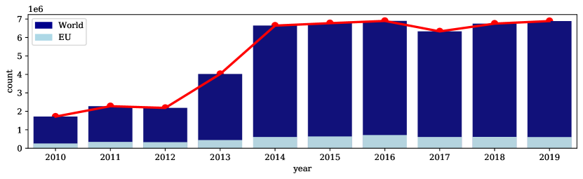
Figure 1: The number of news recorded by Bloomberg each year. For both world and European countries, there is a significant increase in the number of news from 2014.

Schumaker and Chen (2009) use a classical feature engineering method to predict the market behavior. More recently, deep learning methods are more frequently applied on this task. Ding et al. (2014, 2015) employ structured representations to normalize a news then apply a Convolutional Neural Network (CNN) on this formulation. Hu et al. (2018) apply an improved Transformer model (Vaswani et al., 2017) to handle all the words in the raw text simultaneously to predict the forward return. Luss and d’Aspremont (2015) propose a statistical learning method to combine text data and the historical returns. Xu and Cohen (2018) improve the idea from Luss and d’Aspremont (2015) by designing a deep neural network. Ke et al. (2019) adopts a simple but effective classification method combining both regression and Term-Frequency Inversed Document Frequency (TF-IDF) model (Jones, 1972). Del Corro and Hoffart (2020) further introduce an unsupervised method to extract market moving events from text data, which overcomes the problem of lacking reliable labels in financial data.

Before applying computational models mentioned above, the first step usually involves converting words into fixed-length vectors (these fixed-length vectors are called embeddings in natural language processing, details are presented in Section 2.2). Mikolov et al. (2013) propose Word2Vec model to embed words based on words co-occurrence prediction and Pennington et al. (2014) propose a similar GloVe model based on words co-occurrence frequencies. However, both methods can only generate static non-contextualized embeddings. It means that a word is converted to the same vector no matter its meaning or its context. This approach ignores the fact that the meaning of a word can change significantly in different contexts, which impacts the performance of the model. As most of the previous researches rely heavily on static non-contextualized embedding such as Word2Vec or GloVe, there can be accuracy loss.

Cer et al. (2018) and Peters et al. (2018) propose methods to generate contextualized embeddings by jointly considering all the words together. They published their models trained on large English corpus. Although effective, the model is fixed and does not contain domain-specific knowledge in finance.

Devlin et al. (2018) introduce a general-use language model called Bidirectional Encoder Representations from Transformers (BERT). It is one of the most promising models in natural language processing and it showed significant improvement on multiple benchmarks (Wang et al., 2018). The BERT model is pre-trained on a very large scale of textual data to leverage all the features in natural languages, and it also provides the ability to fine-tune this pre-trained model with domain-specific data without needing to start from the scratch. As we have a large amount of financial texts, we can use them to add financial knowledge to the BERT model and generate contextualized embeddings with domain-specific knowledge in finance from BERT.

In addition, previous researches evaluate the performance of the models based on the accuracy calculated on all the news (Ding et al., 2015; Xu and Cohen, 2018; Hu et al., 2018). However, this evaluation metric does not reflect the real capability of the model since investors only care about the news which can move the market significantly. The news identified as neutral have little impact on investors’ decisions, as investors will simply ignore the news if they are classified as neutral.

In this paper, aiming to solve the problems mentioned above, we want our research to have the following characteristics:

• It adopts the contextualized embeddings instead of the static embeddings.

• The contextualized embeddings contain financial domain-specific knowledge.

• Our model has a better prediction on the news which can move the market significantly.

Hence, based on previous work (Sec. 2), we propose Fine-Tuned Contextualized-Embedding Recurrent Neural Network (FT-CE-RNN) to predict the stock price movement based on the headlines (Sec. 3). Using Bloomberg News dataset (Sec. 4), this model generates contextualized embeddings with domain-specific knowledge using all the hidden vectors from the BERT model fine-tuned on financial news. Then FT-CE-RNN uses a recurrent neural network (RNN) to make use of the generated embeddings. (Sec. 5) We also introduce a new evaluation metric which calculates the accuracy on various percentiles of the prediction scores on the test set instead of the whole test set to better incorporate investors’ interests. Our experiments show that our FT-CE-RNN achieves a state-of-the-art performance compared with other baseline models. We also evaluate our model by running trading simulations with different trading strategies. (Sec. 6)

2 Related Work

2.1 Stock Movement Prediction

Stock movement prediction is a widely discussed topic in both finance and computer science communities. Researchers predict the stock market using all available information, including historical stock price, company fundamentals, third-party news sentiment score, financial news, social media texts and even satellite images.

The most classical method is to use the historical stock prices to predict the future prices. Kraft and Kraft (1977); Sonsino and Shavit (2014); Ariyo et al. (2014); Kroujiline et al. (2016); Jiang et al. (2018) use time series analysis techniques to extract the patterns of historical returns, and predict the future stock movement based on these patterns. More recently, researchers start to use neural networks to analyze this pattern (Kohara et al., 1997; Adebiyi et al., 2012; Tashiro et al., 2019; Chen and Ge, 2019; Mäkinen et al., 2019; Bai and Pukthuanthong, 2020).

Financial analysts usually use companies’ fundamental indicators from their financial reports to predict the stocks’ prices in the future (Zhang and Yan, 2018). This includes the use of earnings per share (EPS) (Patell, 1976), debt-to-equity (D/E) ratio (Bhandari, 1988), cash flow (Liu et al., 2007), etc. Nonejad (2021) builds a conditional model to jointly consider historical prices and financial indicators.

With the rapid development of the natural language processing and deep learning, researchers start to focus on predicting stock movement based on textual data, such as financial news and social media texts, which were viewed as difficult to process systematically. Financial news data vendors such as Bloomberg, ThomsonReuters and RavenPack all include their proprietary sentiment analysis on the news. Coqueret (2020) thoroughly analyzes the sentiment classification given by Bloomberg and finds disappointing results on its predicting power. Ke et al. (2019) include the RavenPack’s proprietary score as a benchmark and find it less performing than other models.

Hence, more researchers propose their own natural language processing models to improve the predictability based on financial news. Luss and d’Aspremont (2015) propose an improved Kernel learning method to extract the features in the texts. Ke et al. (2019) use statistical learning methods to determine the sentiment of the words in the news. More recently, computer scientists begin using state-of-the-art deep learning techniques to solve this problem. Ding et al. (2015); Hu et al. (2018); Xu and Cohen (2018); Li et al. (2020) propose different deep learning models to extract information from both financial news and social media texts.

There are also other researches which use uncommon data to predict future stock prices. The data includes key people compensation (Cooper et al., 2016), satellite images (Donaldson and Storeygard, 2016) and the pictures included in the news (Obaid and Pukthuanthong, 2021).

2.2 Contextualized Embedding

In the natural language processing, the first step usually involves transforming words or sentences into fixed-length vectors to allow numerical computations. These fixed-length vectors are known as the embeddings of the words or the sentences.

Historically, researchers use one-hot embeddings (Stevens et al., 1946) to encode words. However, the dimension of the one-hot embedding is large since each unique word takes one dimension. Hence, researchers start to develop methods to make the word embeddings denser.

The most widely used methods for word embedding are Word2Vec (Mikolov et al., 2013) and GloVe (Pennington et al., 2014), both of which are based on word co-occurrences. Such models take in a large number of texts and output a fixed vector for each word in the texts. The more frequently the two words co-occur, the more correlated two embeddings are. Once the model is trained, the embeddings of the words no long change, therefore we call these embeddings static embeddings. Such model generates the same embedding for one word no matter its context, although the meanings of the words can depend on the context in which this word occurs.

Researchers propose contextualized embeddings to solve this issue. Instead of taking only one words as input, the contextualized embedding model accepts the whole sentence as its input. The model then generates the embeddings for each word in the sentence by jointly considering the word and all the other words in the sentence. Cer et al. (2018) proposes Universal Sentence Encoder (USE) to encode the whole sentence contextually. However, USE only gives the embedding of the sentence as a vector without specifying the embedding of each word. Peters et al. (2018) proposed Embeddings from Language Models (ELMo) to embed words based on their linguistic contexts, but ELMo is trained on general English language, making the generated embeddings lack of financial domain-specific knowledge. However, Yang et al. (2020) showed domain-specific model outperforms general models in most of the tasks.

Recent researches on general-use language model such as BERT (Devlin et al., 2018) and XLNet (Yang et al., 2019) reported impressive result on all natural language processing tasks. More interestingly, these models propose a way to fine-tune its pre-trained model on general English with domain-specific data.

Hence, we propose FT-CE-RNN to complement existing researches. FT-CE-RNN generates contextualized embeddings with domain-specific knowledge from the BERT model, it then makes the stock movement prediction based on this more advanced embedding.

3 Problem Formulation

Suppose that we have a stock $s$ with a headline $h_{s,t}$ recorded at time $t$, and the headline has $N$ words, we denote them by $w_{1},...,w_{N}$. We first need to transform them into fixed-length embeddings. Suppose that the length of the embedding is $l_{e}$, this process can be written as:

$$Emb_{i}=f_{s}(w_{i})$$ (1)

where $Emb_{i}\in\mathbb{R}^{l_{e}}$ is the embedding of the word $w_{i}$ and $f_{s}$ denotes the static embedding encoder. In this case, each word has a fixed embedding independent of its context.

A contextualized embedding encoder has the same function of converting a word into a vector, unless it considers all the words in a sentence together. We use $f_{c}$ to denote this contextualized embedding encoder, it can be written as:

$$Emb_{i}=f_{c}(w_{i}|w_{1},...,w_{N})$$ (2)

We concatenate the embeddings of all words to get the embedding of the headline $h_{s,t}$. We define the embedding of this headline as:

$$Emb_{h_{s,t}}=[Emb_{1},...,Emb_{N}]$$ (3)

where $Emb_{h_{s,t}}\in\mathbb{R}^{l_{e}\times N}$.

Following the work of Luss and d’Aspremont (2015); Ding et al. (2015); Xu and Cohen (2018); Ke et al. (2019), we formulate the stock movement prediction as a binary classification task. It means that we predict if a news has a positive impact or a negative impact on the related stock.

We define its market-adjusted return $r_{s,t}$ as

$$r_{s,t}=\frac{P_{s,t+\Delta t}}{P_{s,t}}-\frac{P_{m,t+\Delta t}}{P_{m,t}}$$ (4)

where $P_{s,t}$ denotes the price of stock $s$ at time $t$ and $P_{m,t}$ denotes the value of the equity index at time $t$.

We notice that it is necessary to use market-adjusted return instead of the simple return, as the information contained in the price change is partially due to the information related to this stock (such as news), and also partially due to the information related to other macroeconomic information (such as interest rate, fiscal policies, etc.). As the macroeconomic effect impacts all stocks, it can be explained by a weighted sum of all stocks, such as market index. We can simply remove this impact by subtracting the index return from the stock return, and this adjusted return can better explain the impact of the news.

Most researches in the stock movement prediction based on news simply suppose that all the news induce the market change in the same way (Luss and d’Aspremont, 2015; Xu and Cohen, 2018; Hu et al., 2018; Ke et al., 2019), and therefore use the same $\Delta t$ to calculate the forward returns of all news. However, Fedyk (2018) suggests that the news during the trading hours and the news outside the trading hours have different market impact.

Hence, for different news, we choose different $\Delta t$. For example, for the news published during the trading hours, the price can change in several minutes after the arrival of the news. In this case, we can choose a smaller $\Delta t$ of several minutes or several hours. However, for the news published out of the trading hours, as the market is already closed, we cannot observe the effect of the news until the next market open. Therefore, we need to choose a $\Delta t$ of several days.

We define the stock price movement as:

$$Y_{s,t}=\begin{cases}1,&r_{s,t}>0\\ 0,&r_{s,t}\leq 0\\ \end{cases}$$ (5)

The goal is to predict $Y_{s,t}$ from the embeddings of the headlines $Emb_{h_{s,t}}$. It can be written as:

$$\hat{Y}_{s,t}=g(Emb_{h_{s,t}})$$ (6)

where $g$ represents the prediction model.

4 Data

4.1 Data Description

The dataset that we use is Bloomberg News. In this dataset, each entry contains a timestamp showing when this news is published, a ticker which tells the stock related to this news and the headline of this news. In addition to the necessary information above, there are two fields given by Bloomberg’s proprietary classification algorithm. The score is among -1, 0 and +1, which indicates if the news is either negative, neutral or positive. Confidence is a value between 0 and 100 related to score. A higher confidence value means that Bloomberg’s model is more sure about its score. Bloomberg’s classification will serve as one of the benchmarks for our prediction model. We present a sample dataset in Table 4.1.

A small sample from the Bloomberg News dataset Headline TimeStamp Ticker Score Confidence 1st Source Corp: 06/20/2015 - 1st Source announces the promotion of Kim Richardson in St. Joseph 2015-06-20T05:02:04.063 SRCE -1 39 Siasat Daily: Microsoft continues rebranding of Nokia Priority stores in India opens one in Chennai 2015-06-20T05:14:01.096 MSFT 1 98 Rosneft, Eurochem to cooperate on monetization at east urengoy 2015-06-20T08:01:53.625 ROSN RM 0 98

We need to address that in our dataset, we only have the headlines of the news instead of the whole article.

In our experiment, we use the news data on all the stocks from the STOXX Europe 600 index which represents the 600 largest stocks of the European market. In order not to overfit, we select a short period (from 01/01/2016 to 30/06/2018) as our training set and another short period (from 01/07/2018 to 31/12/2018) as our development set. We tune the parameters of the models only based on this subset of the data, we then test on the whole period (from 01/01/2011 to 31/12/2019) on a 3-year rolling basis. It means that we generate the classification result of the year $y$ using model trained between $y-3$ and $y-1$, without varying the parameters initially obtained. Detailed statistics of the dataset are in Table 4.1. We can also find the number of news in each year from Figure 1.

Statistics of the Bloomberg News dataset Train Dev Test^a Total news 1,616,922 316,944 5,253,345 Word counts 17,650,629 3,554,324 55,410,309 From date 01/01/2016 01/07/2018 01/01/2011 End date 30/06/2018 31/12/2018 31/12/2019

^a Note that we do not simply apply our model trained on the training set on the test set. The training set and the development set are only used to find the hyper-parameters for our models. We generate the scores on test set using different models trained on a 3-year rolling basis, as described in section 4.1

In addition to the Bloomberg news dataset, we also use the cooperate action adjusted share prices at market close and intraday minute bar share prices for all the stocks. The share prices are used to label our data and simulate our trading strategies.

4.2 Data Labelling

For this supervised learning task, we need to provide our model with the ground-truth as its target. However, our data is simply the headlines of the financial news, it does not tell us if a news is positive or negative. Hence, we need to give each news in the training set a label (positive or negative) before training our model.

The intuition behind our labelling method is simply that if a news is positive, the investors will start to overbuy the related stocks, the stock should therefore outperform the market and vice versa. We use Equation 4 to calculate the market adjusted return for each news. As discussed in Section 3, we consider the different effects of the news which occur during the trading hour and those outside the trading hour. We use different $\Delta t$ (Eq. 4) for the news during the trading hours and outside the trading hours. For the news inside trading hours, we choose $\Delta t_{i}$ and for the news outside the trading hours, we use $\Delta t_{e}$. We show an example of the distribution of the returns for all the news in Figure 2.

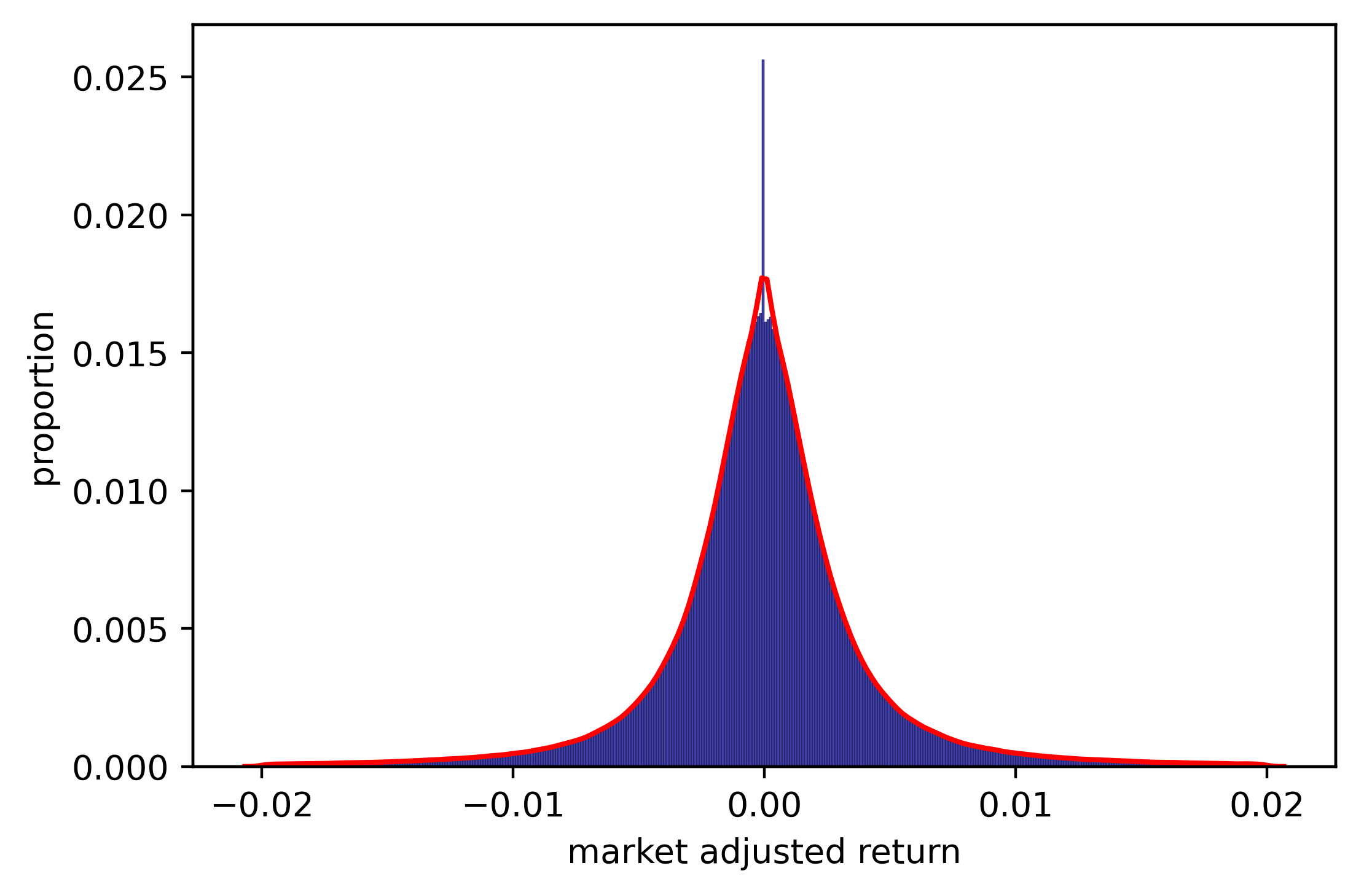
(a) In trading hours

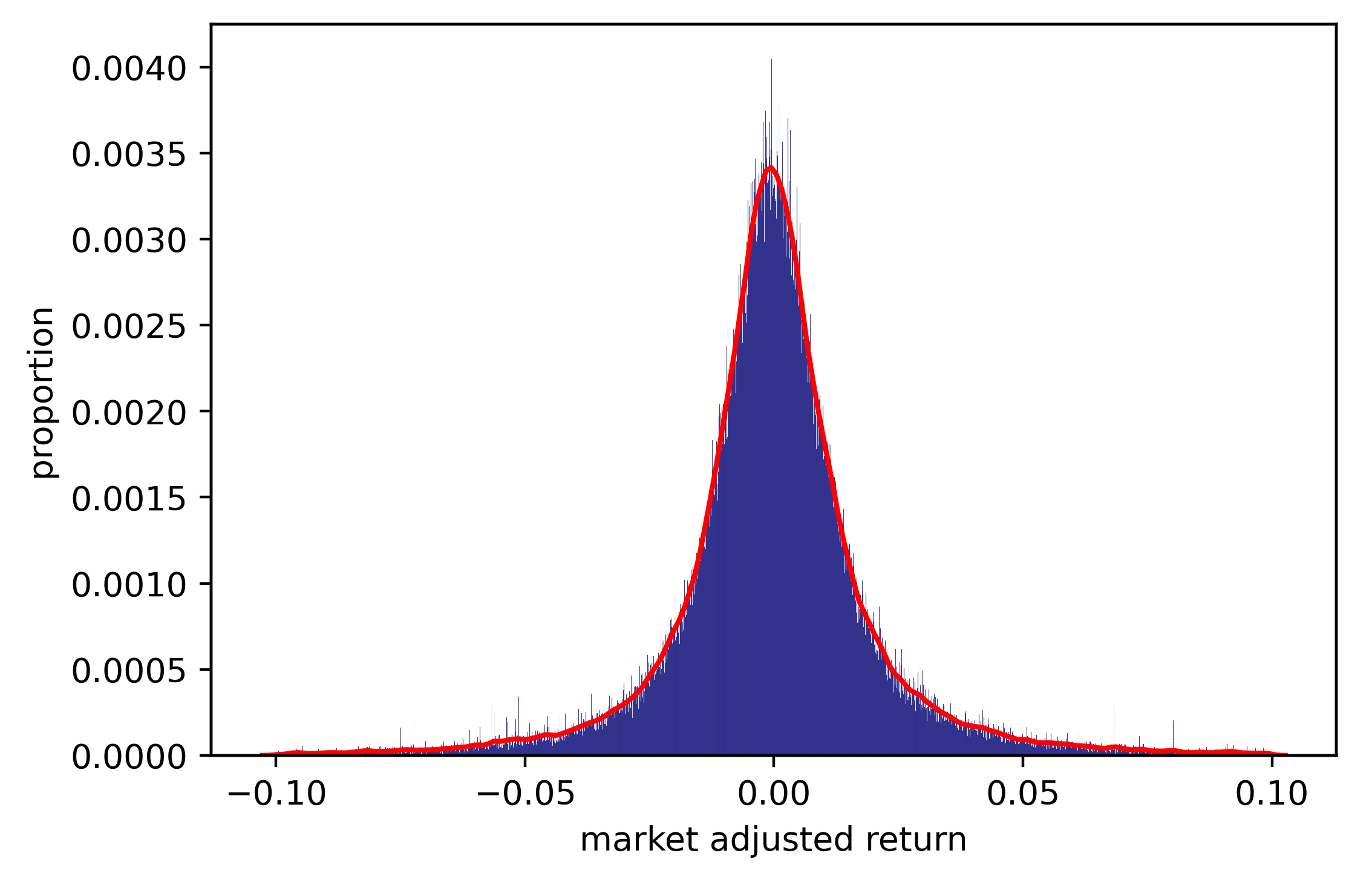
(b) Outside trading hours

Figure 2: The distribution of the $r_{s,t}$ for both the news in the trading hour and those outside the trading hour. The returns are calculated on all the news in the training set. For the news in the trading hour (Figure (a)), we use the forward return of 30 minutes ($\Delta t_{i}=30minutes$), and for those outside the trading hour (Figure (b)), we use the forward return of 1 day($\Delta t_{e}=1day$). We can see that the market adjusted returns are symmetrically distributed.

We label the data based on the market-adjusted return mentioned above. As our task is to identify market-moving news which investors focus on, we need to remove news which do not have significant impact on the price. As we found that the return distribution is quite balanced for the training set (Figure 2), we simply label the 15% news with most positive return as 1 and the 15% news with most negative return as 0. This can be written as:

$$Y_{s,t,train}=\begin{cases}1,&r_{s,t}\ in\ top\ 15\%\\ 0,&r_{s,t}\ in\ bottom\ 15\%\\ removed,&otherwise\\ \end{cases}$$ (7)

where $Y_{s,t,train}$ is the label for the news $e_{s,t}$ for stock $s$ recorded at time $t$ in the training set.

However, for development and test sets, we label all news with positive return as 1 and all news with negative return as 0. This can be written as:

$$Y_{s,t,dev/test}=\begin{cases}1,&r_{s,t}>0\\ 0,&r_{s,t}\leq 0\\ \end{cases}$$ (8)

This difference in labelling is simply to avoid the information leakage. In real-life scenario we cannot know the forward return of a news when it is published. Therefore, we cannot know if the news is in the top 15-percentile or the bottom 15-percentile. We are supposed to give each news a score when it is published regardless its forward return.

However, we can choose to exclude a news according to its score when calculating the metrics, as this information is available immediately after we receive the news. We use this idea to construct different test sets to evaluate of model. We present the details in Section 6.2.

5 Prediction Model

There are two main components in our model: a contextualized embedding encoder from BERT model and a Recurrent Neural Network (RNN) which takes the contextualized embedding as input and outputs the classification probability for both classes.

5.1 Contextualized Embedding Encoder from BERT

The Bidirectional Encoder Representations from Transformers (BERT) proposed by Devlin et al. (2018) is a widely used language model in the natural language processing applications. It is first pre-trained on very large scale data (WikiBooks and Wikipedia) to learn the basic characteristics of a language. After this pre-training phase, we can obtain a pre-trained base BERT model for all other downstream tasks (such as text classification). This pre-training process is computationally intensive, we simply use the pre-trained BERT model published by Google.

Figure 3 shows the structure of BERT model. It has $L$ layers and each layer has $N$ nodes, each node is a Transformer (Vaswani et al., 2017). The first layer takes a tokenized headline as input and the BERT model generates $N\times L$ hidden vectors, denoted by $T_{i,j}$. The first token at the first layer is a special [CLS] token reserved for fine-tuning.

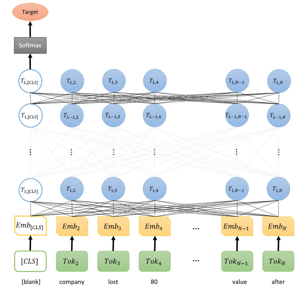
Figure 3: BERT model with input headline ”company lost about 80 percent of its market value after interim data” and the maximum length of model is set to 10 ($N=10$). The last two words interim and data are therefore trimmed. There are $L$ layers in this BERT model. $Tok_{i}$ denotes the i-th token of the tokenized news and $N$ denotes the maximum length of a headline. $T_{i,j}$ represents the hidden vector for the $j$-th transformer at layer $i$. The first [CLS] label is simply a special string we choose to signify the class of this headline. This label is only used when fine-tuning the model, we leave it blank when we generate the embeddings. The original method to use BERT as classification model is to use directly [CLS] vector to represent the whole sentence, while we choose to use all hidden vectors at one layer to represent the sentence. The embedding generated with the model is shown in Equation 11.

For a specific downstream task, we can fine-tune the base BERT model suitable for this specific task. It means that we do not initialize the parameters of BERT model randomly, we use the pre-trained BERT model as our initial state instead. We update the parameters in the base model with our domain-specific data. This approach adds domain knowledge to the large scale language model (Yang et al., 2020), it can help the BERT model better understand the texts in specific situations. In our case, we can fine-tune the base BERT model with our labelled financial news data mentioned in Section 4.2 to make it specialize in financial texts.

The fine-tuning process is straightforward. We input the class label (0 or 1) together with the tokenized headline into the first layer of a pre-trained BERT model. We set the target to the class label and loss function to cross-entropy, defined as:

$$loss=\sum Y_{i}ln(P_{i}^{+})+(1-Y_{i})ln(1-P_{i}^{+})$$ (9)

where $Y_{i}$ is the label for the news $i$ and $P_{i}^{+}$ denotes the probability that the news $i$ is positive given by the model. We use back-propagation (Hecht-Nielsen, 1992) to update the parameters in the model. We repeat such operation for several epochs until the loss converges.

In order to generate the contextualized embedding, we can either directly use the base BERT model or use the fine-tuned model. We first tokenize our headlines using SentencePiece tokenizer (Kudo and Richardson, 2018). If the number of tokens is smaller than $N$, we simply pad it to $N$ tokens by adding null tokens at the end. If there are more than $N$ tokens, we remove the last tokens to make this sentence have exactly $N$ tokens. We input these tokens into pre-trained BERT model as shown in Figure 3 with the first token which stands for [CLS] label left blank. Suppose that our BERT model has $L$ layers, we can then generate $L$ different embeddings, denoted by $Emb_{base,l}$. We have,

$$Emb_{base,l}=[T_{l,2},T_{l,3},...,T_{l,N}]$$ (10)

where $Emb_{base,l}$ is a $size(T_{l,i})\times(N-1)$ matrix representing this headline and $l$ denotes the layer from which we generate the embedding. We have $1\leq l\leq L$.

Similarly, we can generate another $L$ embeddings from the fine-tuned BERT model, denoted by $Emb_{tuned,l}$. We have,

$$Emb_{tuned,l}=[T_{l,2}^{{}^{\prime}},T_{l,3}^{{}^{\prime}},...,T_{l,N}^{{}^{\prime}}]$$ (11)

where $T_{l,i}^{{}^{\prime}}$ denotes the hidden vector for the i-th token at the l-th layer for the fine-tuned model.

5.2 RNN Prediction Model

The structure of our prediction model is simple and straightforward, it is shown in Figure 4.

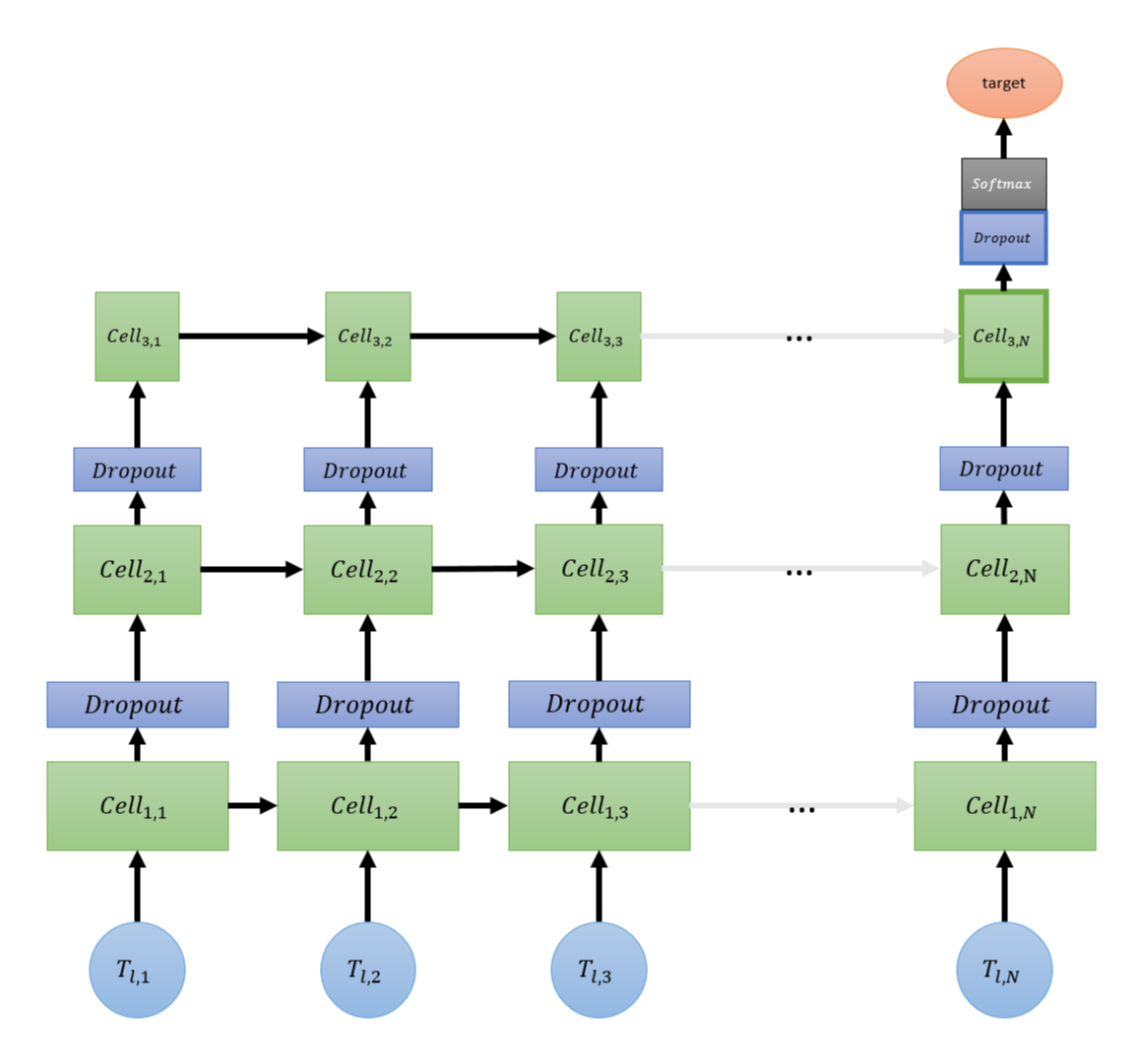
Figure 4: Structure of our RNN network. $Cell_{i,j}$ denotes the j-th cell on the i-th layer. The cell can be either Vanilla RNN, LSTM or GRU. In addition, the output size reduces when it approaches the last layer of the model.

There are several layers of cells which can either be Vanilla RNN (Cleeremans et al., 1989), Long-Short Term Memory (LSTM) (Hochreiter and Schmidhuber, 1997) or Gated Recurrent Unit (GRU) (Cho et al., 2014). The size of output at each layer shrinks in order to reduce the dimension of our features gradually and to make the remaining features more meaningful. Two neighbor layers are connected by a dropout to overcome the overfitting problem in the network. At the end of the last layer, a softmax is added to calculate the probability for each class based on the last vector on the last layer.

Suppose that we choose to use $Emb_{base,l}$ to represent a sentence. We first initialize the parameters in the RNN model randomly and input the embeddings of tokens ($T_{l,i}$) sequentially into the cells ($Cell_{1,i}$) in the first layer of the recurrent neural network. At the same time, we set the target to the corresponding label of the headline. We use the same cross-entropy loss mentioned in Equation 10 as our loss function. We use the same back propagation procedure in Section 5.1 to update the parameters in the model until we have a stable loss.

6 Experiments

In this section, we introduce our experiment setup and results in detail. We also include the results of some baseline models to prove the effectiveness of our model. In addition to the final result, we add some ablation experiment results to show the effect of some factors in our model.

6.1 Training Setup

We use the pre-trained 12-layer, 768-dimension, 12-heads BERT model to generate $E_{base,l}$, then we fine-tune this base model using our labelled dataset with the method mentioned in section 4.2. We choose the best-performing fine-tuned model to generate $E_{tuned,l}$. Empirically, the layer of BERT used as embedding should not be too close to the first layer, otherwise the contextualized embedding will be too similar to the static embedding. Hence, we only test embeddings with $l=L,L-1\ or\ L-2$. This choice will be discussed in detail in Section 6.6.

The maximum length of a sentence is set to 32 tokens, as there are at most 29 tokens for all headlines in our dataset. If there are fewer tokens, we pad it to 32 with null tokens.

For our RNN model, the cells are set to be LSTM. We use a four-layer single-directional RNN with a dropout rate of 50%.

6.2 Evaluation Metrics

Because of the huge volume of news that we receive daily, it is not realistic for either human investors or systematic trading algorithms to react on all news. Otherwise, we lose a considerable amount of transaction fees on the news which do not significantly move the market. It is more logical that an investor first reads the news, then buys or sells the stock if he thinks that the news can have substantial impact on the stock price. If he thinks that the news is neutral, he will simply ignore the news. In this type of neutral-insensitive scenario, evaluating our model on all news is less meaningful. Instead, we evaluate our model only on certain ”extreme” news chosen based on their sentiment classification results.

We define the score of a news, denoted by $S_{news}$:

$$S_{news}=(P_{+}(news)-0.5)\times 2$$ (12)

where $P_{+}(news)$ denotes the probability that this news belongs to the positive class given by the prediction model. $S_{news}$ is therefore a value between -1 and 1.

We use $P_{n}$ to denote the $n^{th}$ percentile of all scores on the training set. We can then choose the set on which we want to evaluate our model. We define this set $E_{2n}$ by:

$$E_{n}^{-} =\{news|S_{news}<P_{n}\}$$ (13)

$$E_{n}^{+} =\{news|S_{news}>P_{100-n}\}$$

$$E_{2n} =E_{n}^{-}\cup E_{n}^{+}$$

We assume that the distributions of scores on the training set and the test set are the same. It should contain about $n\%$ highest-score news and $n\%$ lowest-score news from the test set. We evaluate our model on these subsets of news instead of all news in the test set.

Standard Metrics

Given a confusion matrix $\bigl{(}\begin{smallmatrix}tp&fn\\ fp&tn\end{smallmatrix}\bigr{)}$ which contains the number of samples classified as true positive ($tp$), false positive ($fp$), true negative ($tn$) and false negative ($fn$). We use both the accuracy and the Matthews Correlation Coefficient (MCC) (Matthews, 1975) to evaluate our models. These two values are defined by:

Accuracy:

$$\frac{tp+tn}{tp+tn+fp+fn}$$ (14)

Matthews Correlation Coefficient (MCC):

$$\frac{tp\times tn-fp\times fn}{\sqrt{(tp+fp)(tp+fn)(tn+fp)(tn+fn)}}$$ (15)

Trading Strategies

However, those two metrics introduced above do not perfectly reflect the reality, as the profits are quite different when the price goes up significantly or mildly, although they are both counted as true positive. Hence, it is necessary to simulate these trades on real markets. We use two simple trading strategies for simulations.

Strategy 1 (S1).

We simply follow the strategy used by Ke et al. (2019).

Before each market close, we search for all the news belonging to $E_{n}$ with a maximum age of $A$ days. We group the selected news by stock and we calculate the average score for each stock. We choose the 20 stocks with the highest scores, our target position for these stocks is $T. We also choose the 20 stocks with the lowest scores, our target position for these stocks is -$T.

Strategy 2 (S2).

The advantage of S1 is that it perfectly balances the long leg and the short leg. As such, we have no exposure to the market, and it reduces the risk of the market movement. However, the fallback of S1 is that it only focuses on the highest scores instead of considering all the stocks. In this case, we will not be able to fully use our predictions. Hence, we design the following strategy to solve this problem:

1. We first calculate the average score for each stock using the same method as described in S1.

2. We choose all the stocks with positive scores, $s_{i}^{+}$ denotes the score for the stock $i$.

3. The target position for the stock $i$ is $\$20T\times s_{i}^{+}/\sum_{j}s_{j}^{+}$.

4. We invest in the stocks with negative scores in the same way. For a negatively scored stock $i$, we invest $-\$20T\times s_{i}^{-}/\sum_{j}s_{j}^{-}$.

This strategy not only uses all the available classification results, but also has no exposure to the market as S1, since the long position and the short position are both $20T$.

To evaluate the performance of these strategies, we use the following two commonly used indicators in finance.

Annualized return: defined by

$$\frac{1}{N}\sum_{t=1}^{N}r_{t}\times D$$ (16)

where $D$ is the number of trading days in one year, and $r_{t}$ denotes the daily return of the portfolio for the day $t$, defined by the ratio of the profit on day $t$ to the total position on day $t$.

Annualized Sharpe Ratio: defined by

$$\frac{\overline{\textbf{r}}}{\sigma(\textbf{r})}\times\sqrt{D}$$ (17)

$\overline{\textbf{r}}$ denotes the mean of all the $r_{i}$ and $\sigma(\textbf{r})$ represents the standard deviation all the $r_{i}$.

6.3 Baselines and Proposed Models

We use the following models as baselines.

• NBC (Maron, 1961): Naive Bayes Classifier

  One of the most traditional language classification models based on word frequency.

• SSESTM (Ke et al., 2019): Supervised Sentiment Extraction via Screening and Topic Modeling.

  A regression model based on word frequency and stock returns.

• Bloomberg (Proprietary): Bloomberg Sentiment Score

  The sentiment score from Bloomberg’s proprietary model, which comes along with the Bloomberg News dataset. An example of this sentiment score is shown in Table 4.1.

• BERT (Devlin et al., 2018): Bidirectional Encoder Representations from Transformers

  A general and powerful language model for a wide range of NLP tasks. We directly use the [CLS] label as the final prediction, as proposed by the author.

• FinBERT (Yang et al., 2020): Financial Sentiment Analysis with BERT

  The same structure as the BERT model but pre-trained with financial domain-specific data.

To make a detailed analysis of the improvement brought by our proposed models, in addition to the final version of our model (FT-CE-RNN), we add two other intermediate variants of our RNN model.

• RNN: Recurrent Neural Network

  The recurrent neural network introduced in Section 5.2. Instead of using contextualized embeddings, we use the static Word2Vec embedding as its first layer.

• CE-RNN: Contextualized Embedding - Recurrent Neural Network.

  The network structure is the same as RNN, but we use contextualized embedding generated from base BERT model instead of Word2Vec.

• FT-CE-RNN: Fine-Tuned - Contextualized Embedding - Recurrent Neural Network

  The same RNN using contextualized embedding generated from fine-tuned BERT.

6.4 Results

The detailed results for standard metrics are shown in Table 6.4 and Figure 5. We also list the results from trading simulations in Table 6.4.

Performance of baseline models and our proposed RNN variants evaluated in accuracy and MCC 1%^a 2% 5% 10% Acc MCC Acc MCC Acc MCC Acc MCC NBC 59.8 0.2 56.1 0.12 54.3 0.09 53.4 0.07 SSESTM 56.3 0.13 55.4 0.11 54.4 0.09 53.2 0.06 Bloomberg ^b 58.3 0.42 58.3 0.42 58.0 0.34 54.5 0.31 BERT 73.6 0.46 66.5 0.45 59.3 0.43 56.1 0.42 FinBERT 73.9 0.46 66.5 0.45 59.2 0.43 55.6 0.42 RNN 71.4 0.45 63.4 0.44 56.7 0.43 54.3 0.42 CE-RNN 70.9 0.42 63.8 0.28 57.9 0.16 54.7 0.09 FT-CE-RNN 74.5 0.48 67.8 0.45 59.3 0.44 56.6 0.43

^a1% signifies that we test our result on $E_{1}$, which includes about 1% of all news on the test set. ^bIn Bloomberg dataset, we have about 4% of the news with a maximum level score, therefore we have the same result for $E_{1}$ and $E_{2}$.

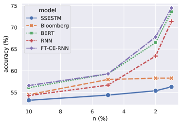
(a) Accuracy

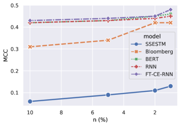
(b) MCC

Figure 5: Accuracy and MCC results of different models varied with $E_{n}$, the horizontal axis represents the value of $n$

Performance of baselines and proposed models in trading simulations^a Strategy Model 1% 2% 5% Ret.^b Sharpe Ret. Sharpe Ret. Sharpe S1 NBC 9.61 1.09 2.35 0.26 2.44 0.27 SSESTM 2.39 0.41 1.57 0.24 2.74 0.35 Bloomberg 8.83 1.19 8.83 1.19 8.03 1.10 BERT 9.33 1.42 8.08 1.11 8.21 1.09 FinBERT 8.83 1.22 8.29 1.10 7.86 1.13 RNN 9.86 1.43 8.06 1.13 6.43 0.89 CE-RNN 8.39 1.07 7.31 0.99 7.62 1.01 FT-CE-RNN 10.75 1.50 12.31 1.70 11.32 1.50 S2 NBC 7.93 0.62 0.57 0.06 0.80 0.15 SSESTM 4.75 0.47 3.02 0.35 2.76 0.38 Bloomberg 10.76 1.61 10.76 1.61 9.82 1.56 BERT 13.10 1.42 11.42 1.56 9.87 1.53 FinBERT 11.35 1.24 9.85 1.21 12.85 1.97 RNN 17.53 1.75 15.47 1.72 12.70 1.79 CE-RNN 12.58 1.33 10.37 1.25 8.29 1.05 FT-CE-RNN 19.72 2.11 18.39 2.49 15.01 2.31

^aThe simulation does not consider transaction costs. ^bThe annualized return, presented in percent.

We find that in terms of accuracy, our FT-CE-RNN outperforms all the other baselines models. Especially, comparing the accuracy of RNN and FT-CE-RNN, there is an improvement of 4.1% when we test on the 1% most extreme news ($E_{1}$). This result shows the power of contextualized embedding against static embedding. We also notice that there is an improvement of 0.9% compared with BERT result. This result explains that using all hidden vectors instead of only one [CLS] vector helps improve the result. However, if we directly use the embedding from the base BERT (CE-RNN) instead of the fined-tuned BERT (FT-CE-RNN), there is a clear disadvantage. This result shows the necessity of including the domain knowledge in the embeddings.

In addition, we observe that all our models have a significant margin compared with the Bloomberg and SSESTM sentiment score, which is completely independent of our data labelling and modelling process, this result can prove the efficiency of our models compared with other widely used models in the industry.

In our trading simulations, we use a look-back window of 5 days ($A=5\ days$). We find that the result of our FT-CE-RNN outperforms all other models in most of the cases. The most significant improvement is on Sharpe Ratio. When trading on the 1% most extreme news using strategy S2, there is an improvement of 0.69 (49%) in Sharpe ratio and an improvement of 6.62 (51%) in return if we compare BERT and FT-CE-RNN. It means that our model using contextualized embedding is not only more profitable but also more stable.

We can also find that S2 performs better than S1, since S2 uses all the signals while S1 only uses the signals on the top/bottom stocks. This proves that our classification is valid for most of the stocks, making it a robust method.

An example of trading simulation is shown in Figure 6. It shows how our profit evolves with time. We observe that FT-CE-RNN is not only better on profitability and stability but also on the absolute profit in dollars.

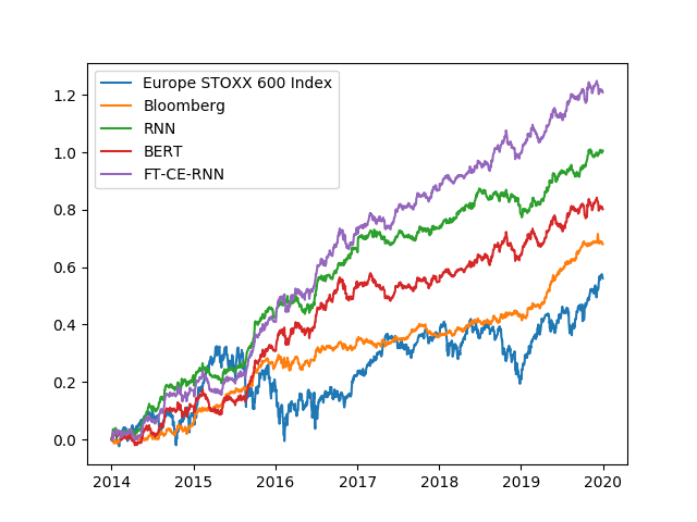
Figure 6: Trading simulation result in absolute profit. This trading simulation is run on 1% most extreme news ($E_{1}$) using strategy S2. We also include the market return, represented by Europe STOXX 600 Index. We can see our models largely exceed the market return and the Bloomberg sentiment score.

6.5 Transaction costs

Trading simulation results with transaction costs^a Model No cost With cost Ret. Sharpe Ret. Sharpe NBC 7.93 0.62 2.09 0.16 SSESTM 4.75 0.47 -1.80 -0.18 Bloomberg 10.76 1.61 4.49 0.67 BERT 13.10 1.42 5.98 0.65 FinBERT 11.35 1.24 3.88 0.42 RNN 17.53 1.75 11.57 1.15 CE-RNN 12.58 1.33 6.15 0.65 FT-CE-RNN 19.72 2.11 12.60 1.35

^aThe result is obtained based on $E_{1}$ test set using the trading strategy S2.

Our trading simulations ignore transaction costs thus far, since the primary goal of this research is to prove the effectiveness of our sentiment model with contextualized embedding. The transaction costs have no impact on the result because all the models are in the same no-cost environment.

That said, applying this model in real-life trading is another separate but interesting question. To understand the real gain of our FT-CE-RNN model for the asset management, we rerun our trading simulations with transaction costs.

In our simulations, we assume a transaction cost of 4bps proportional to the daily turnover. The simulation results with transaction costs are shown in Table 6.5.

Although the transaction costs cut our profits significantly, we can still have a profitable margin when using our FT-CE-RNN model.

6.6 Effect of Embedding Layer

In this section, we discuss our choice of BERT hidden layer to be used as embedding.

Empirically, the final layer of BERT model should be used to generate our contextualized embedding as the final layer is more ”mature” and contains more information compared with other layers which are closer to the first layer. However, our result listed in Table 6.6 shows the opposite.

Accuracy result using different layers of BERT model as contextualized embedding^a Embedding layer $L$^b $L-1$ $L-2$ CE-RNN 70.9 68.1 63.3 FT-CE-RNN 73.0 74.5 66.7

^aThe result is acquired on the $E_{1}$ test set. ^b$L$ denotes the last layer of the BERT model, $L-n$ represents the $n$-th last layer of the BERT model.

We find that the best result for CE-RNN is acquired when we use layer $L$ while the best result for FT-CE-RNN is obtained when using layer $L-1$. The reason for this phenomenon is that the last layer of the fine-tuned BERT is biased towards the classification result, since the goal for the fine-tuning process is to make the first token of the last layer close to the classification target. If we use the last layer of the fine-tuned BERT as the input for RNN, we are simply replicating the classification process of the BERT, instead of improving the result. Using one deeper layer ($L-1$) helps reduce this bias (Xiao, 2018). However, the base BERT does not have this bias on the last layer since it has no previous knowledge on the training set. This explains why CE-RNN has a better performance when using the embedding from the last layer ($L$).

If we use an even lower layer to generate contextualized embedding, such as $L-2$, the performance declines as it is too close to the embedding layer and lacks contextualized characteristics.

6.7 Effect of Classification Classes

During our initial researches, we also explored the possibility of using a 3-class classification instead of a 2-class classification. It means that we do not classify a news into a positive or a negative news, we classify if a news is either positive, negative or neutral. This is the method adopted in the Bloomberg’s proprietary model.

The accuracy result for a 2-class classification model and a 3-class classification model^ab Acc 1% 2% 5% 10% 2-class 74.5 67.8 59.3 56.6 3-class 61.0 58.4 55.5 53.6

^aThe result is based on the test set $E_{1}$. ^bFor 3-class classification, we choose the $n/2$% largest scores for the positive class and the $n/2$% largest scores for the negative class as our $E_{n}$. The guarantees the same number of the news considered in both cases.

The result of using a 3-class classification model is shown in Table 6.7. We find a significant worse performance if we add another possibility to our model. This is because a 3-class model supposes a clear difference between the market-moving news and the neutral news, however, this is not always the case. It is not obvious to find a threshold, above which the news is positive and below which the news is neutral. In this scenario, we are not able to construct a clear training set for our model to learn the difference between a neutral news and a market-moving news.

Hence, in our final model, we decide to classify the news into two classes instead of three.

6.8 Qualitative Analysis of the Classification Result

We analyze the news in $E_{1}$ to see if there is any pattern, for example, some frequent words in them. We include the 50 most frequent words appeared in $E^{+}_{0.5}$ and 50 most frequent words in $E^{-}_{0.5}$ in Appendix 8, along with their frequencies. We exclude all the stopwords in English, such as to, for, a, etc.

We can find that for the news identified as the most positive, some common words include buy, upgrade, raise, etc. For the news identified as the most negative, downgrade, cut and miss are among common words. These are also logical keywords for the humans, making the result from the neural network intuitive.

We can also find in this collection that there are also some less natural words, such as fly, say neutral, etc. However, as these words appear in both categories, the effect of such words is neutralized if we empirically assume the effect of a word is its positive impact minus its negative impact.

This result is similar to the result we get from the word frequency-based method, such as NBC and SSESTM. However, we demonstrate that our FT-CE-RNN model is significantly more powerful than these two baseline models (Section 6.4). This phenomenon implies that our model is capable of capturing complex information in the news on top of the word frequency.

7 Conclusion

We build the whole pipeline for the stock movement prediction task with headlines from financial news, including labeling the news, generating contextualized embedding, training a neural network model, validating the model with various metrics and building trading strategies based on the model output.

We design a FT-CE-RNN model which uses fine-tuned contextualized embeddings from BERT instead of the traditional static embeddings. We also introduce our new evaluation metrics focusing on market-moving news, which are more suitable for asset manager’s needs.

Through various experiments on the Bloomberg News dataset, we demonstrate the effectiveness of our FT-CE-RNN model. We find a better performance, in both accuracy and trading simulations, than other widely used baseline models. We also include other ablation studies to discuss the choice of some important parameters and to demonstrate the intuitiveness of the result.

In the future, we will continue our research on the stock movement prediction using natural language processing methods based on longer texts (such as earning call transcripts, financial reports, etc.) instead of the headlines. By using more information, we aim to build a model which helps achieve better stock movement prediction result.

8 Frequent Words in Market Moving News

The most frequent words in the most positvely scored news and the most negatively scored news positive negative word frequency word frequency buy 0.0344 downgraded 0.0252 upgraded 0.0187 cut 0.0240 deal 0.0172 fly 0.0173 said 0.0172 bank 0.0142 raised 0.0158 misses 0.0110 fly 0.0131 falls 0.0106 order 0.0107 neutral 0.0092 talks 0.0094 hold 0.0092 gets 0.0075 cuts 0.0088 neutral 0.0071 sell 0.0086 raises 0.0065 buy 0.0078 wins 0.0054 miss 0.0078 hold 0.0054 estimates 0.0073 billion 0.0053 outlook 0.0061 street 0.0052 sales 0.0058 stake 0.0048 profit 0.0054 unit 0.0047 earnings 0.0054 insider 0.0046 tradegate 0.0050 buyback 0.0041 says 0.0049 outlook 0.0038 sees 0.0043 offer 0.0037 downgrades 0.0036 agrees 0.0036 shares 0.0036 buys 0.0035 revenue 0.0035 says 0.0034 underperform 0.0029 group 0.0032 underweight 0.0029 berenberg 0.0030 credit 0.0028 near 0.0029 close 0.0028 sell 0.0029 lower 0.0027 bid 0.0026 results 0.0027 tradegate 0.0026 loss 0.0025 approval 0.0025 leave 0.0025 new 0.0025 forecast 0.0023 buyout 0.0025 guidance 0.0022 bank 0.0025 growth 0.0022 acquire 0.0025 overweight 0.0021 outperform 0.0024 negative 0.0020 rises 0.0023 downgrade 0.0020 worth 0.0023 outperform 0.0020 eu 0.0022 loses 0.0019 contract 0.0022 weight 0.0019 close 0.0021 seeking 0.0019 overweight 0.0020 drops 0.0018 credit 0.0020 equal 0.0018 set 0.0019 close 0.0017 fiat 0.0018 new 0.0017 gains 0.0018 perform 0.0017 sees 0.0017 indicated 0.0016 merger 0.0017 price 0.0016 takeover 0.0016 target 0.0016

References

- Adebiyi et al. (2012) Adebiyi, A.A., Ayo, C.K., Adebiyi, M.O. and Otokiti, S.O., Stock price prediction using neural network with hybridized market indicators. Journal of Emerging Trends in Computing and Information Sciences, 2012, 3, 1–9.
- Ariyo et al. (2014) Ariyo, A.A., Adewumi, A.O. and Ayo, C.K., Stock price prediction using the ARIMA model. In Proceedings of the 2014 UKSim-AMSS 16th International Conference on Computer Modelling and Simulation, pp. 106–112, 2014.
- Bai and Pukthuanthong (2020) Bai, Y. and Pukthuanthong, K., Machine Learning Classification Methods and Portfolio Allocation: An Examination of Market Efficiency. Available at SSRN 3665051, 2020.
- Bhandari (1988) Bhandari, L.C., Debt/equity ratio and expected common stock returns: Empirical evidence. The journal of finance, 1988, 43, 507–528.
- Cer et al. (2018) Cer, D., Yang, Y., Kong, S.y., Hua, N., Limtiaco, N., John, R.S., Constant, N., Guajardo-Céspedes, M., Yuan, S., Tar, C. et al., Universal sentence encoder. arXiv preprint arXiv:1803.11175, 2018.
- Chen and Ge (2019) Chen, S. and Ge, L., Exploring the attention mechanism in LSTM-based Hong Kong stock price movement prediction. Quantitative Finance, 2019, 19, 1507–1515.
- Cho et al. (2014) Cho, K., Van Merriënboer, B., Bahdanau, D. and Bengio, Y., On the properties of neural machine translation: Encoder-decoder approaches. arXiv preprint arXiv:1409.1259, 2014.
- Cleeremans et al. (1989) Cleeremans, A., Servan-Schreiber, D. and McClelland, J.L., Finite state automata and simple recurrent networks. Neural computation, 1989, 1, 372–381.
- Cooper et al. (2016) Cooper, M.J., Gulen, H. and Rau, P.R., Performance for pay? The relation between CEO incentive compensation and future stock price performance. The Relation Between CEO Incentive Compensation and Future Stock Price Performance (November 1, 2016), 2016.
- Coqueret (2020) Coqueret, G., Stock-specific sentiment and return predictability. Quantitative Finance, 2020, 20, 1531–1551.
- Del Corro and Hoffart (2020) Del Corro, L. and Hoffart, J., Unsupervised Extraction of Market Moving Events with Neural Attention. arXiv preprint arXiv:2001.09466, 2020.
- Devlin et al. (2018) Devlin, J., Chang, M., Lee, K. and Toutanova, K., BERT: Pre-training of Deep Bidirectional Transformers for Language Understanding. CoRR, 2018, abs/1810.04805.
- Ding et al. (2014) Ding, X., Zhang, Y., Liu, T. and Duan, J., Using structured events to predict stock price movement: An empirical investigation. In Proceedings of the Proceedings of the 2014 Conference on Empirical Methods in Natural Language Processing (EMNLP), pp. 1415–1425, 2014.
- Ding et al. (2015) Ding, X., Zhang, Y., Liu, T. and Duan, J., Deep learning for event-driven stock prediction. In Proceedings of the Twenty-Fourth International Joint Conference on Artificial Intelligence, 2015.
- Donaldson and Storeygard (2016) Donaldson, D. and Storeygard, A., The view from above: Applications of satellite data in economics. Journal of Economic Perspectives, 2016, 30, 171–98.
- Fama (1965) Fama, E.F., The behavior of stock-market prices. The journal of Business, 1965, 38, 34–105.
- Fedyk (2018) Fedyk, A., Front page news: The effect of news positioning on financial markets. Technical report, working paper, 2018.
- Hecht-Nielsen (1992) Hecht-Nielsen, R., Theory of the backpropagation neural network. In Neural networks for perception, pp. 65–93, 1992, Elsevier.
- Hochreiter and Schmidhuber (1997) Hochreiter, S. and Schmidhuber, J., Long short-term memory. Neural computation, 1997, 9, 1735–1780.
- Hu et al. (2018) Hu, Z., Liu, W., Bian, J., Liu, X. and Liu, T.Y., Listening to chaotic whispers: A deep learning framework for news-oriented stock trend prediction. In Proceedings of the Proceedings of the Eleventh ACM International Conference on Web Search and Data Mining, pp. 261–269, 2018.
- Jiang et al. (2018) Jiang, Z.Q., Wang, G.J., Canabarro, A., Podobnik, B., Xie, C., Stanley, H.E. and Zhou, W.X., Short term prediction of extreme returns based on the recurrence interval analysis. Quantitative Finance, 2018, 18, 353–370.
- Jones (1972) Jones, K.S., A statistical interpretation of term specificity and its application in retrieval. Journal of documentation, 1972.
- Ke et al. (2019) Ke, Z.T., Kelly, B.T. and Xiu, D., Predicting returns with text data. Technical report, National Bureau of Economic Research, 2019.
- Kohara et al. (1997) Kohara, K., Ishikawa, T., Fukuhara, Y. and Nakamura, Y., Stock price prediction using prior knowledge and neural networks. Intelligent Systems in Accounting, Finance & Management, 1997, 6, 11–22.
- Kraft and Kraft (1977) Kraft, J. and Kraft, A., Determinants of common stock prices: a time series analysis. The journal of finance, 1977, 32, 417–425.
- Kroujiline et al. (2016) Kroujiline, D., Gusev, M., Ushanov, D., Sharov, S.V. and Govorkov, B., Forecasting stock market returns over multiple time horizons. Quantitative Finance, 2016, 16, 1695–1712.
- Kudo and Richardson (2018) Kudo, T. and Richardson, J., SentencePiece: A simple and language independent subword tokenizer and detokenizer for Neural Text Processing. CoRR, 2018, abs/1808.06226.
- Li et al. (2020) Li, J., Li, G., Zhu, X. and Yao, Y., Identifying the influential factors of commodity futures prices through a new text mining approach. Quantitative Finance, 2020, 20, 1967–1981.
- Liu et al. (2007) Liu, J., Nissim, D. and Thomas, J., Is cash flow king in valuations?. Financial Analysts Journal, 2007, 63, 56–68.
- Luss and d’Aspremont (2015) Luss, R. and d’Aspremont, A., Predicting abnormal returns from news using text classification. Quantitative Finance, 2015, 15, 999–1012.
- Mäkinen et al. (2019) Mäkinen, Y., Kanniainen, J., Gabbouj, M. and Iosifidis, A., Forecasting jump arrivals in stock prices: new attention-based network architecture using limit order book data. Quantitative Finance, 2019, 19, 2033–2050.
- Maron (1961) Maron, M.E., Automatic indexing: an experimental inquiry. Journal of the ACM (JACM), 1961, 8, 404–417.
- Matthews (1975) Matthews, B.W., Comparison of the predicted and observed secondary structure of T4 phage lysozyme. Biochimica et Biophysica Acta (BBA)-Protein Structure, 1975, 405, 442–451.
- Mikolov et al. (2013) Mikolov, T., Sutskever, I., Chen, K., Corrado, G.S. and Dean, J., Distributed representations of words and phrases and their compositionality. In Proceedings of the Advances in neural information processing systems, pp. 3111–3119, 2013.
- Nguyen and Shirai (2015) Nguyen, T.H. and Shirai, K., Topic modeling based sentiment analysis on social media for stock market prediction. In Proceedings of the Proceedings of the 53rd Annual Meeting of the Association for Computational Linguistics and the 7th International Joint Conference on Natural Language Processing (Volume 1: Long Papers), Vol. 1, pp. 1354–1364, 2015.
- Nonejad (2021) Nonejad, N., Bayesian model averaging and the conditional volatility process: an application to predicting aggregate equity returns by conditioning on economic variables. Quantitative Finance, 2021, pp. 1–25.
- Obaid and Pukthuanthong (2021) Obaid, K. and Pukthuanthong, K., A picture is worth a thousand words: Measuring investor sentiment by combining machine learning and photos from news. Journal of Financial Economics, 2021.
- Oliveira et al. (2013) Oliveira, N., Cortez, P. and Areal, N., Some experiments on modeling stock market behavior using investor sentiment analysis and posting volume from Twitter. In Proceedings of the Proceedings of the 3rd International Conference on Web Intelligence, Mining and Semantics, p. 31, 2013.
- Pagolu et al. (2016) Pagolu, V.S., Reddy, K.N., Panda, G. and Majhi, B., Sentiment analysis of Twitter data for predicting stock market movements. In Proceedings of the 2016 international conference on signal processing, communication, power and embedded system (SCOPES), pp. 1345–1350, 2016.
- Patell (1976) Patell, J.M., Corporate forecasts of earnings per share and stock price behavior: Empirical test. Journal of accounting research, 1976, pp. 246–276.
- Pennington et al. (2014) Pennington, J., Socher, R. and Manning, C.D., GloVe: Global Vectors for Word Representation. In Proceedings of the Empirical Methods in Natural Language Processing (EMNLP), pp. 1532–1543, 2014.
- Peters et al. (2018) Peters, M.E., Neumann, M., Iyyer, M., Gardner, M., Clark, C., Lee, K. and Zettlemoyer, L., Deep contextualized word representations. arXiv preprint arXiv:1802.05365, 2018.
- Rekabsaz et al. (2017) Rekabsaz, N., Lupu, M., Baklanov, A., Hanbury, A., Dür, A. and Anderson, L., Volatility prediction using financial disclosures sentiments with word embedding-based ir models. arXiv preprint arXiv:1702.01978, 2017.