Empirical evidence on the Euler equation for investment in the US

Abstract

Is the typical specification of the Euler equation for investment employed in DSGE models consistent with aggregate macro data? Using state-of-the-art econometric methods that are robust to weak instruments and exploit information in possible structural changes, the answer is yes. Unfortunately, however, there is very little information about the values of these parameters in aggregate data because investment is unresponsive to changes in capital utilization and the real interest rate. In DSGE models, the investment adjustment cost and the persistence of the investment-specific technology shock parameters are mainly identified by, respectively, the cross-equation restrictions and the dynamics implied by the structure of the model.

Keywords: Investment, Adjustment costs, Weak identification.

JEL classification: C2, E22.

1 Introduction

An important component of the demand side of standard Dynamic Stochastic General Equilibrium (DSGE) models is aggregate investment. The seminal contribution by Christiano et al. (2005) proposes an investment-adjustment cost model coupled with the assumption of variable capital utilization to capture the inertial response of aggregate investment to monetary policy shocks. This specification for investment behavior has become standard in the DGSE literature, and the implied Euler equation for investment features in most DSGE models used for policy analysis. The key structural parameters of this investment block of modern DSGE models are: the investment adjustment cost parameter that denotes the inverse of the elasticity of investment with respect to the shadow price of capital, the elasticity of the capital utilization cost function, and the persistence of the investment-specific technology shock.

However, estimates of these three key parameters differ greatly across papers in the literature. The next Section shows that different parameter values entail a very different response of investment, and hence of output, to various shocks. Not surprisingly, this then translates to different implications regarding the main drivers of business cycle fluctuations, in terms of the relative importance of the various shocks. Hence, these parameters are key for our interpretation of the business cycle through the lens of the investment block of a standard DSGE model. It seems important, therefore, to investigate why the estimates of the key parameters vary greatly and how accurately they can be estimated using aggregate macro data. This is what we do in this paper. More specifically, we ask the following two questions.

First, is the typical specification of the Euler equation for investment employed in DSGE models together with an autoregressive investment-specific shock consistent with aggregate macro data? We test the bare minimum implications of this model with state-of-the-art generalized method of moments (GMM) tests, and we find that the answer is yes. In other words, there is no evidence against this specification that can be found in aggregate macro data. This is a positive message that we add to the literature. We are not aware of any paper in the literature that checks the consistency of the implied Euler equation for investment with aggregate data as a single equation, rather than through the lens of Bayesian estimation of a full DSGE model. We use recently developed econometric methods in Magnusson and Mavroeidis (2014) and in Mikusheva (2021) to deal with weak identification. The former incorporates subsample information in the data arising from structural changes in the economy such as policy regime shifts. These methods also serve as parameter stability tests that are fully robust to weak instruments, and, hence, they provide reliable evidence on the stability of the parameters over the sample. The latter explores information of all potential instruments available for inference using a split-sample technique. Moreover, using the common assumption of variable capital utilization to derive our estimated equation allows us, on the one hand, to avoid issues of using proxies for unobservable variables, such as the return on capital or the Tobin’s marginal Q, and, on the other hand, to use observable variables, such as the real interest rate and capacity utilization that is fully consistent with the investment block currently used in modern DSGE modeling. Finally, the single-equation approach is robust to potential misspecification in other equations of the system.

The second question is: how much can we learn from aggregate time series data about the values of the three key parameters mentioned above? Unfortunately, the answer to this second question is not much. The structural parameters of the investment equation are generally very poorly identified, that is, there is very little information about these parameters in aggregate data. Using typical lagged values of the endogenous variables as instruments, the confidence sets contain almost the entire parameter space. This motivates us to consider external sets of instruments, such as oil prices, financial uncertainty measures, government expenditure shocks and monetary policy shocks; however, we find that they help very little in identifying the main structural parameters. Then, we present the implications of this finding in terms of possible ranges of the impulse response functions and of the variance decompositions using the standard medium-scale DSGE model of Justiniano et al. (2010) (JPT, henceforth). Our analysis shows that the results are particularly sensitive to the value of the investment adjustment cost parameter and the persistence of the investment-specific technology shock. Hence, it seems that pinning down these two parameters is key and more important than identifying a value for the elasticity of capital utilization.

The above finding of weak identification contrasts with the results typically reported in the DSGE literature, leading us to investigate how DSGE models could achieve identification of these parameters (again using the JPT model). This can be achieved in two ways, either through the prior or through the joint model dynamics of the variables in the system and the related cross-equation restrictions implied by rational expectations. Both features differentiate the DSGE estimation from our method. While estimating a system of equations could help identification through cross-equation restrictions, possible misspecification in other parts of the model could lead to biased estimates. Our analysis suggests the following. Consistent with our GMM results, the elasticity of the capital utilization cost function is not identified by the data, so identification is largely due to the prior. On the other hand, the investment adjustment cost parameter is mainly identified by the cross-equation restrictions implied by the structure of the DSGE model, when using the JPT model and data set. The persistence parameter of the investment-specific shock is always high and well identified, even if we relax some of the cross-equation restrictions and use a loose prior. We conjecture this to be due to the fact that the model wants to match the very persistent dynamics of the observable macroeconomic time series.

Finally, we estimate a semi-structural model parameterized in terms of the slope coefficients of the investment equation with respect to the capital utilization rate and the real interest rate. We show that, when the persistence of the investment-specific technology shock is large, the semi-structural parameters corresponding to the above slope coefficients are not well-identified. Weak identification arises because the change in the capital utilization rate and the real interest rate are poorly forecastable. In contrast, when the persistence of the investment-specific technology shock is low, these slope parameters can be well-identified. However, because the confidence sets on those semi-structural parameters cover zero, and the mapping from the semi-structural to the structural parameters is ill-posed near zero, the structural parameters are weakly identified - small changes in the slope coefficients generate large changes in the capital utilization and investment adjustment cost parameters. Overall, the semi-structural analysis suggests that investment is unresponsive to the real interest rate and to capital utilization. Therefore, at a technical level, we conclude that it is the mapping from semi-structural to structural parameters that prevents the identification of the latter. Finally, comparing our results to those in Magnusson and Mavroeidis (2014), structural change is not as informative for the identification of the Euler equation for investment as it is for the NKPC. This is in line with the results in Ascari et al. (2021), suggesting again that policy regime shifts have had more impact on nominal variables than on real variables over our sample.

Our paper could be of interest to any researchers using the standard investment cost specification proposed by Christiano et al. (2005) in their medium-scale DSGE models. The literature is immense and a small subset of influential papers are considered in Figure 1 below. Our paper is also related to the literature that estimates individual equations employed in standard DSGE models using GMM methods and aggregate data. Specifically, three equations have been extensively studied on their own: the New Keynesian Phillips Curve (Galí and Gertler, 1999), the Taylor rule (Clarida et al., 2000), and the Euler equation for consumption (Yogo, 2004). The present paper is the first to conduct a similar exercise for the other main component of the demand side of modern DSGE models: investment.

Finally, our contribution and results are also complementary to the literature that estimates investment functions using cross-sectional microeconomic data of firms. There is a very large literature mainly concerned with additional costs of external financing as a result of information asymmetries and agency costs. This external financing cost may increase the sensitivity of investment decisions to sources of internal finance such as cash flows for constrained firms (Fazzari et al., 1988). Groth and Khan (2010) and Eberly et al. (2012) are, instead, very closely related to our work because they estimate the investment adjustment-cost model of Christiano et al. (2005) on 18 industries and on firm-level data, respectively. Groth and Khan (2010) focus on the estimation of the adjustment cost parameter and find that to be very small in U.S. manufacturing industries, implying that investment is highly sensitive to the current shadow value of capital, in contrast to the aggregate estimates from well-known DSGE models reported in Figure 1, see Groth and Khan (2010, Table 5). Eberly et al. (2012) instead focus on investigating the importance of the lagged investment term implied by the Christiano et al. (2005) specification. They report a strong and robust lagged-investment effect in their estimates, implying inertial dynamics of investment for the set of firms in their sample. Our approach here is very different as we want to assess the ability to identify the parameters of the investment block of DSGE models from aggregate data. As such, we also use the common assumption of variable capital utilization to derive our estimated equation. Our macroeconomic approach abstracts from heterogeneous adjustment costs or elasticities of investment, since this would require modelling the heterogeneity of firms at the micro level.

The structure of the paper is as follows. Section 2 presents the theoretical specification and it investigates the implication of using different values for the parameters of the investment equation, as taken from influential papers in the DSGE literature. Section 3 describes the econometric methodology and Section 4 presents the data. Section 5 presents the empirical results. Section 6 discusses the identification of the key parameters of the investment equation in DSGE models, in light of our results. Section 7 concludes. Additional empirical results, data sources and econometric methods are reported in the Appendix.

2 The Euler equation of investment and DSGE models

The investment equation used in our empirical investigation comes from the most standard specification used in medium-scale DSGE models. Since the seminal paper by Christiano et al. (2005), DSGE models commonly employ the assumption of investment adjustment costs (IAC) and variable capital utilization. Investment pertains to the demand side of the model and the first-order conditions are commonly derived from the households’ problem, assuming that households take investment decisions, own the capital stock and rent capital to the firms. A representative household’s lifetime utility, separable in consumption, $C_{t}$, and hours worked, $L_{t}$, is expressed as

$$E_{0}\sum_{t=0}^{\infty}\beta^{t}U(C_{t},L_{t}),$$ (1)

where $\beta$ is the discount factor. The household’s period t budget constraint is

$$C_{t}+I_{t}+\dfrac{B_{t+1}}{P_{t}}\leq\dfrac{R_{t-1}B_{t}}{P_{t}}+\dfrac{W_{t}L_{t}}{P_{t}}+\Pi_{t}+r_{t}^{k}u_{t}\hat{K}_{t}-a(u_{t})\hat{K}_{t},$$ (2)

where $I_{t}$ is investment, $B_{t}$ is the amount of risk-free bonds that pay a nominal gross interest rate of $R_{t}$, $W_{t}$ is the nominal wage, $\Pi_{t}$ denotes firms’ profits net of lump-sum taxes, $r_{t}^{k}$ is the real rental rate of capital, $\hat{K}_{t}$ is the physical capital stock, and $a(u_{t})$ is the function that measures the cost of capital utilization per unit of physical capital. Capital owning households choose the capital utilization rate, $u_{t}$, that transforms physical capital $\hat{K}_{t}$ into effective capital ${K}_{t}$ as follows

$$K_{t}=u_{t}\hat{K}_{t}.$$ (3)

Effective capital is rented to intermediate goods producers at the rate $r_{t}^{k}$. Standard assumptions are: i) $\bar{u}=1$ and $a(\bar{u})=0$, where a bar over a variable denotes its steady state value; ii) the curvature of the function $a(u)$, given by $a^{\prime\prime}(u)/a^{\prime}(u)$, measures the elasticity of capital utilization cost and it is such that $\zeta=a^{\prime\prime}(1)/a^{\prime}(1)>0$.

The representative household accumulates end-of-period $t$ capital according to a standard capital accumulation equation

$$\hat{K}_{t+1}=\nu_{t}\left[1-\mathcal{S}\left(\dfrac{I_{t}}{I_{t-1}}\right)\right]I_{t}+(1-\delta)\hat{K}_{t},$$ (4)

where $\delta$ is the depreciation rate and $\nu_{t}$ is the investment-specific technology shock, that is, a shock to the efficiency with which the final good can be transformed into physical capital, as in JPT. The log of the investment shock follows the autoregressive stochastic process $\log\nu_{t}=\rho\log{\nu_{t-1}}+\varepsilon_{t}^{v}$, where $\rho$ is the autoregressive coefficient.

The IAC is specified as

$$\mathcal{S}\left(\dfrac{I_{t}}{I_{t-1}}\right)I_{t}=\dfrac{\kappa}{2}\left(\dfrac{I_{t}}{I_{t-1}}-1\right)^{2}I_{t}.$$ (5)

where the IAC function $\mathcal{S}(\cdot)$ is such that $\mathcal{S}(1)=\mathcal{S}^{\prime}(1)=0$ with $\kappa=\mathcal{S}^{\prime\prime}(1)>0$. Here, $\kappa$, the adjustment cost parameter, denotes the inverse of the elasticity of investment with respect to the shadow price of capital. There are no adjustment costs at the steady state when $I$ is fixed.

The representative household chooses ${I_{t},}$ ${u_{t},}$ ${\hat{K}_{t+1},}$ and ${B_{t+1}}$ to maximise (1) under the period-by-period budget constraint (2) and capital accumulation equation (4). Appendix A shows how log-linearizing the first-order conditions of this problem and rearranging them yields the following dynamic equation for investment

$$\Delta\widetilde{i}_{t}=\left(\beta+\phi_{q}\right)E_{t}\Delta\widetilde{i}_{t+1}-\beta\phi_{q}E_{t}\Delta\widetilde{i}_{t+2}+\dfrac{1}{\kappa}\left[\phi_{k}\zeta E_{t}\widetilde{u}_{t+1}-\widetilde{r}_{t}^{p}+\widetilde{\nu}_{t}\right]-\dfrac{\phi_{q}}{\kappa}E_{t}\widetilde{\nu}_{t+1}.$$ (6)

Lowercase letters with a tilde denote the respective log deviations of the variables from their steady state, $\widetilde{r}_{t}^{p}$ denotes the log-deviation of the ex-ante real interest rate from steady state, and $\phi_{q}=(1-\delta)\beta$ and $\phi_{k}=1-\phi_{q}$. Intuitively, investment depends positively on expected capital utilization ($E_{t}\widetilde{u}_{t+1}$), negatively on the real interest rate ($\widetilde{r}_{t}^{p}$) and positively on the current value of the investment-specific shock ($\widetilde{\nu}_{t}$). The assumed specification of the adjustment cost makes investment depend on its own one-period lag ($\widetilde{i}_{t-1}$) and its expected leads ($E_{t}\widetilde{i}_{t+1},E_{t}\widetilde{i}_{t+2}$).

Figure 1 shows that estimates of the two main parameters of the Euler equation for investment, i.e., the elasticity of capital utilization cost ($\zeta$) and the investment adjustment cost ($\kappa$), vary widely across various well-known papers in the literature that estimate medium-scale DSGE models.

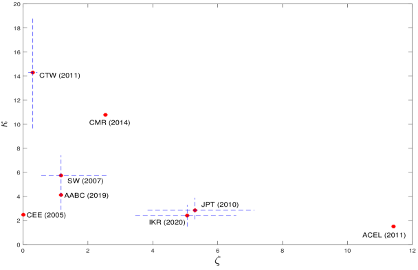
Figure 1: Estimates of the elasticity of capital utilization cost ($\zeta$) and the investment adjustment cost ($\kappa$) including the 90% credible intervals from the literature: Christiano et al. - CEE(2005), Smets and Wouters - SW(2007), Justiniano et al. - JPT(2010), Altig et al. - ACEL(2011), Christiano et al. - CTW(2011), Christiano et al. - CMR(2014), Arias et al. - AABC(2020), Inoue et al. - IKR(2020).

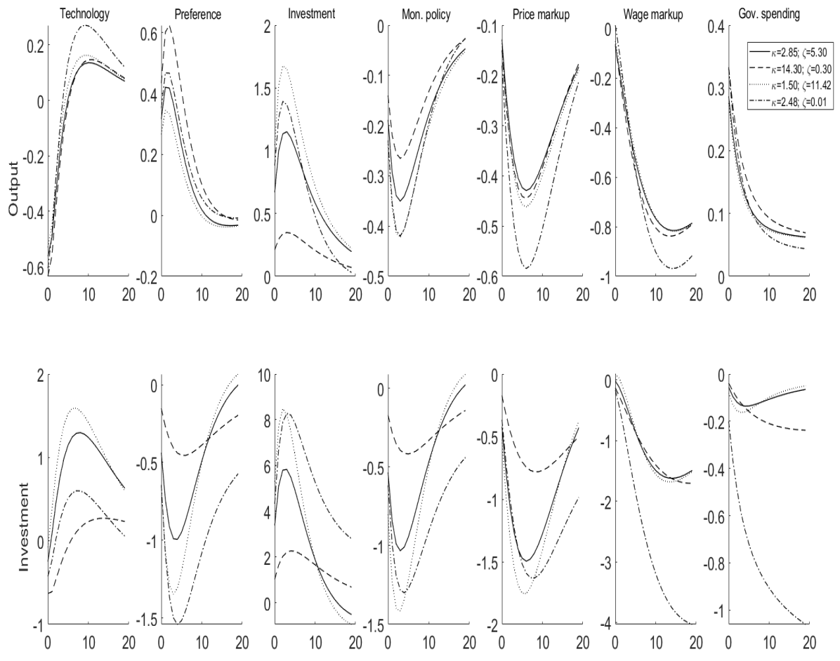
Figure 2: Impulse responses of output and investment to a one-standard deviation structural shock in JPT’s model for alternative calibration of $\kappa$ and $\zeta$. The remaining parameters are set at the posterior median estimate of JPT.

To appreciate the implications of the different values of the parameters characterizing the investment equation we use the JPT model. Figure 2 shows how the impulse responses of output and investment to the seven structural shocks in JPT’s model change when we keep all the parameters fixed at the JPT posterior median, while we vary the value of $\kappa$ and $\zeta$ using the following four values from the literature (see Figure 1) : (i) Justiniano et al. - JPT(2010): $\kappa=2.85$ and $\zeta=5.30$; (ii) Christiano et al. - CTW(2011): $\kappa=14.30$ and $\zeta=0.30$; (iii) Altig et al. - ACEL(2011): $\kappa=1.50$ and $\zeta=11.42$; (iv) Christiano et al. - CEE(2005): $\kappa=2.48$ and $\zeta=0.01.$ It is evident that the response of investment to the various shocks varies substantially from a quantitative point of view in terms of impact effect, peak response and persistence. With the exception of the technology shock, a larger value of $\kappa$ tends to dampen the response of investment. The different responses of investment then translates into different responses in output. As a consequence, these different calibrations have an impact on the variance decomposition of output growth, as shown in Table 1. Not surprisingly, then a large value of $\kappa$ decreases the importance of the investment-specific shock as a driver of the business cycle. The ACEL calibration exhibits the smallest value of the investment adjustment cost parameter ($\kappa=1.5$) and the highest contribution of the investment-specific shock to the variance of output growth (69%) among the four different calibrations. In contrast, the CTW calibration exhibits the largest value of the investment adjustment cost parameter ($\kappa=14.3$) and the lowest contribution of the investment-specific shock to the variance of output growth (8%). The difference in the explained output growth variance is distributed mainly to the preference, technology and government spending shock. Hence, the main result in JPT, for example, about the investment-specific shock being the major driver of the business cycle relies on a relatively low value for $\kappa$, as also discussed by JPT. The effects of different values for $\zeta$ are more difficult to grasp from this analysis, but more will be said about it below. Another crucial parameter for investment fluctuations is the persistence of the investment-specific shock, $\rho$. Figure 3 shows the impulse responses of output and investment to an investment shock in JPT (2010) for grid values of $\rho$ between zero and one - using their posterior median values for $\kappa$ and $\zeta$. Not surprisingly, the larger the value of $\rho$, the larger and more persistent the response of output and investment. Given the relevance of these parameters for our understanding and for the narrative of investment and business cycle fluctuations, it is important to understand the diversity of estimates reported in the literature and investigate whether GMM can pin down the value of these parameters more accurately.

Table 1: Variance decomposition of output growth in JPT’s model

Parameters	Tec	Pref	Inv	MP	PM	WM	Govt
JPT: $\kappa=2.85,\zeta=5.30$	0.21	0.10	0.49	0.04	0.03	0.05	0.07
CTW: $\kappa=14.30,\zeta=0.30$	0.31	0.29	0.08	0.03	0.04	0.10	0.14
ACEL: $\kappa=1.50,\zeta=11.42$	0.14	0.04	0.69	0.04	0.02	0.03	0.04
CEE: $\kappa=2.48,\zeta=0.01$	0.18	0.08	0.55	0.04	0.03	0.06	0.06

• Notes: Justiniano et al. - JPT(2010), Christiano et al. - CTW(2011), Altig et al. - ACEL(2011), Christiano et al. - CEE(2005). Shocks: Technology (Tec), Preference (Pref), Investment (Inv), Monetray Policy (MP), Price markup (PM), Wage markup (WM), Governement spending (Govt).

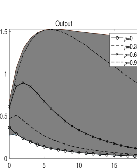
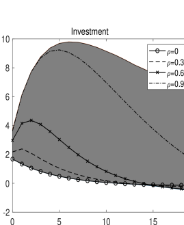
Figure 3: Impulse responses of output and investment to a one-standard deviation investment shock in JPT’s model evaluated at the posterior median of all parameters except $\rho$. The shaded area shows the range of IRFs for $\rho\in[0,1)$.

3 Econometric Methodology

This Section describes the methods we use to estimate the model given in equation (6). Without a complete specification of a DSGE model that includes equation (6), the expectations on its right-hand side are unobserved. Therefore, we need to rely on a limited-information estimation method, such as single-equation GMM. The latter involves replacing the expected future terms in (6) with their realized values and finding valid instruments for them, which are typically predetermined variables. However, in this case, we first need to quasi-difference the equation to remove the autocorrelation in $\widetilde{\nu}_{t}$ that would otherwise rule out using predetermined variables as instruments. Specifically, removing expectations and quasi-differencing equation (6) yields

$$\left[1+\rho\left(\beta+\phi_{q}\right)\right]\Delta\widetilde{i}_{t}= \ \rho\Delta\widetilde{i}_{t-1}+\left[\beta+\phi_{q}+\rho\beta\phi_{q}\right]\Delta\widetilde{i}_{t+1}-\beta\phi_{q}\Delta\widetilde{i}_{t+2}$$

$$+\frac{\phi_{k}\zeta}{\kappa}\widetilde{u}_{t+1}-\frac{\rho\phi_{k}\zeta}{\kappa}\widetilde{u}_{t}-\dfrac{1}{\kappa}\widetilde{r}_{t}^{p}+\rho\dfrac{1}{\kappa}\widetilde{r}_{t-1}^{p}+\epsilon_{t},$$ (7)

where $\epsilon_{t}$ is an error term defined in equation (22) in Appendix A. The time series properties of the residual term $\epsilon_{t}$ are crucial for the selection of valid instruments. It can be gauged from equation (22) that, under rational expectations, $\epsilon_{t}$ is a moving average process of order 2 that consists of current values of the investment adjustment cost shock $\varepsilon_{t}^{\nu}$ and current and future forecast errors of inflation, investment and capital utilization. Hence, it is orthogonal to any predetermined variables.

We estimate the structural parameters in the baseline equation (7) using the generalized method of moments (GMM) framework proposed by Hansen and Singleton (1982), with orthogonality conditions obtained from the assumption that the residuals, $\epsilon_{t}$, in the baseline equation (7) are uncorrelated with any predetermined variables $Z_{t}$. In our estimation, we set $\beta=0.99$ and $\delta=0.025$, and compute confidence sets for the remaining structural parameters $\theta=(\rho,\kappa,\zeta)$.

Our econometric analysis relies solely on methods of inference that are robust to the presence of potential weak instruments, while allowing for heteroskedasticity and autocorrelation in the residuals. We estimate confidence sets based on the S test of Stock and Wright (2000). The S set is constructed as follows. We specify a grid of points within the parameter space. For each of these points, we test whether the identifying restrictions of the model hold using a Wald-type test (Stock and Wright, 2000, call this the S test). All the points in the grid that have not been rejected by a 10% level S test make up the 90% confidence S set.

In addition to the S sets, we also estimate confidence sets based on a test proposed by Magnusson and Mavroeidis (2014), the quasi-local level S (qLL-S) test. The qLL-S set combines the average information on the moment conditions over the sample, which is what the S set uses, with information on the validity of the moment conditions over subsamples. It can be thought of as using subsample information as additional instruments. This subsample information is relevant in two cases: (i) when the parameters of the model are unstable, or (ii) when the parameters of the model are constant but there is time variation in other parts of the economy, for example, monetary policy regime shifts. In case (i), the qLL-S test can be interpreted as a structural change test that is robust to weak identification; therefore a nonrejection is an indication of parameter stability. In case (ii), the qLL-S can have more power than the corresponding S test if the information that comes from structural change elsewhere in the economy is sufficiently strong. Hence, in either case, the qLL-S sets usefully complement the S sets.

The orthogonality condition $E_{t-1}(\epsilon_{t})=0$ in (7) implies that any predetermined variable could be used as an instrument. Therefore, the number of potential instruments is unbounded. However, the S and qLL-S sets may be unreliable if the number of instruments is large relative to the sample size. Therefore, we keep the number of instruments small when we compute S and qLL-S sets. This may be inefficient if information is spread over a large number of instruments, or if the most informative instruments are excluded from the set of instruments that we use. To address this possibility, we use a split-sample S set. This is a straightforward extension of a method recently proposed by Mikusheva (2021) to obtain reliable inference in linear instrumental variables models with time series data and a large number of possibly weak instruments. In Section B of the Appendix we present information about computation of the S, qLL-S and split-sample S tests.

4 Data

We use quarterly aggregate time series data for the US over the period 1967q1 to 2019q4. We consider two proxies for Investment ($I_{t}$). One corresponds to Fixed Private Investment as in Smets and Wouters (2007) (SW, henceforth) , while the other proxy is the sum of Gross Private Domestic Investment and Personal Consumption Expenditure on Durable Goods following JPT. Both investment measures are in real per capita terms and deflated using their respective implicit price deflators. For the nominal interest rate $r_{t}$, we use the quarterly average of the effective Federal Funds rate, and inflation $\pi_{t}$ is obtained from the GDP deflator as $\pi_{t}=\log(P_{t}/P_{t-1})$. The ex-post real interest rate $r_{t}^{p}$ is defined as $r_{t}^{p}=r_{t}-\pi_{t+1}$. For capital utilization ($u_{t}$), we use the Federal Reserve Board’s time series on capacity utilization, which measures the intensity with which all factors of production are used in the industrial production sector (Christiano et al., 2005). When estimating equation (7), we use the log values of investment and capacity utilization, that is, $i_{t}=\log(I_{t})$ and $u_{t}=\log(U_{t})$.

Other variables included in the set of predetermined/exogenous variables $Z_{t}$ are Romer and Romer’s monetary policy shock, Ramey and Zubairy’s military news shock, oil price inflation and (financial) uncertainty measure VXO. Detailed description of the data, its sources and transformations are given in Appendix C.

5 Results

This Section presents first the results of our baseline estimation. Then, we report results based on external instruments, followed by results obtained from combining both lagged endogenous and exogenous instruments together and employing the split-sample method proposed by Mikusheva (2021) that is robust to many weak instruments. Finally, we define a semi-structural model to estimate the slope coefficients of the investment equation with respect to the capital utilization rate and the real interest rate.

5.1 Baseline Estimation

Following the previous studies on the estimation of the consumption Euler equation (Yogo, 2004; Ascari et al., 2021), we begin by investigating the baseline specification equation (7) using one lagged value of the variables that appear in the model as the set of instrumental variables, namely $\Delta{i}_{t-1}$, $r_{t-2}^{p}$, and ${u}_{t-1}$. We keep the number of instruments small to avoid problems associated with the use of many instruments, see Andrews and Stock (2007). We estimate the model using both the SW and the JPT definitions of investment discussed in Section 4. Three-dimensional confidence sets for the parameters $\theta=(\rho,\kappa,\zeta)$ are obtained by considering the ranges $[0,1)\times(0,20]\times(0,10]$ in line with previous studies, see Figure 1. The results are reported in Figure 4.

SW Investment JPT Investment (a) (b) S sets          (c) (d) qLL-S sets         

Figure 4: 90% S and qLL-S confidence sets for $\theta=(\rho,\kappa,\zeta)$ derived from the investment Euler equation model (7). Instruments: constant, $\Delta i_{t-1}$, $r_{t-2}^{p}$, $u_{t-1}$. The investment proxies are Fixed Private Investment (left column) and the sum of Gross Private Domestic Investment and Personal Consumption Expenditure on Durable Goods (right column). Newey and West (1987) HAC. Period: 1967Q1-2019Q4.

Figures 4 (a) and (b) report 90% S sets for the parameters $\rho,\kappa,\zeta$ using SW and JPT investment proxies, respectively. In both cases, the S sets comprise almost the entire parameter space. The only part rejected by the data are small values of $\kappa$ and $\zeta$ when $\rho<1$. The good news from this result is that the investment equation is not rejected by the aggregate data. Nevertheless, the data is essentially uninformative over a very large part of the parameter space. The results remain essentially unchanged when considering two lags instead of one lag for each of the three instruments (see Figure 14 in the Appendix). Additionally, the qLL-S sets reported in Figures 4 (c) and (d) are very similar to the S sets, indicating no presence of parameter instability or violation of the moment conditions in subsamples. Hence, there is minimal information arising from the restrictions on the dynamics of the data to identify the investment equation. As a consequence of the lack of identification, all previous parameter estimates reported in Figure 1 are included in the confidence sets, that is, those estimates are potentially valid values of the true underlying structural parameters of the investment Euler equation (7).

5.2 External Instruments

Given the findings in Figure 4, we explore a more extensive set of information contained in contemporaneous external instruments. These instruments include (i) the monetary policy shock of Romer and Romer (2004), (ii) the military news shock of Ramey (2011, 2016) and updated by Ramey and Zubairy (2018), which captures news about changes in military spending, (iii) changes in the (log) oil price, and (iv) the (standardized) S&P 100 Volatility Index (VXO), which is a proxy for (financial) uncertainty shocks. Some of the external instruments do not cover the entire period. We, therefore, use the longest available sample when estimating the confidence sets. Apart from oil price, the external instruments are in levels. We use the contemporaneous values as instruments.

To keep the number of instruments comparable to Figure 4, we report results in which $r_{t-2}^{p}$ is replaced by an external instrument, or $r_{t-2}^{p}$ and ${u}_{t-1}$ are replaced by a pair of the external instruments. For completeness, we also report results using all of the external instruments together. The resulting S and qLL-S confidence sets are reported in Figures 5 and 6 for the SW and JPT investment proxies, respectively. To facilitate comparison across cases, we report the baseline results at positions (a) and (i) in those figures.

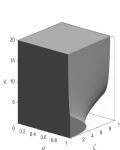
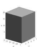
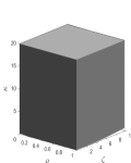
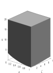
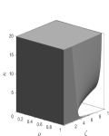
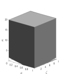
Exogenous Instruments with SW Investment Proxy Baseline Mon. pol. shock Military news Oil 1967Q1-2019Q4 1969Q2-2007Q4 1967Q1-2015Q4 1967Q1-2019Q4 (a) (b) (c) (d) S sets       VXO (b)+(c) (d)+(e) (b)+(c)+(d)+(e) 1967Q1-2019Q4 1969Q2-2007Q4 1967Q1-2019Q4 1969Q2-2007Q4 (e) (f) (g) (h) S sets       Baseline Mon. pol. shock Military news Oil 1967Q1-2019Q4 1969Q2-2007Q4 1967Q1-2015Q4 1967Q1-2019Q4 (i) (j) (k) (l) qLL-S sets       VXO (j)+(k) (l)+(m) (j)+(k)+(l)+(m) 1967Q1-2019Q4 1969Q2-2007Q4 1967Q1-2019Q4 1969Q2-2007Q4 (m) (n) (o) (p) qLL-S sets      

Figure 5: 90% S and qLL-S confidence sets for $\theta=(\rho,\kappa,\zeta)$ derived from the investment Euler equation model (7) using Fixed Private Investment as investment proxy. A constant and $\Delta i_{t-1}$ are common instruments in all specifications while $u_{t-1}$ enters only in specifications (a) to (e) and (i) to (m). The additional instrument(s) by specification is (are): Baseline $r_{t-2}^{p}$; Mon. pol. shock: Romer and Romer’s (2004) monetary policy shock; Military news: Ramey and Zubairy’s (2018) military news shock; Oil: growth rate of real oil price; VXO: financial uncertainty.

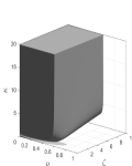
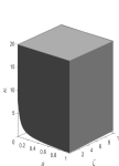
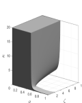
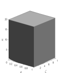
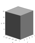
Exogenous Instruments with JPT Investment Proxy Baseline Mon. pol. shock Military news Oil 1967Q1-2019Q4 1969Q2-2007Q4 1967Q1-2015Q4 1967Q1-2019Q4 (a) (b) (c) (d) S sets       VXO (b)+(c) (d)+(e) (b)+(c)+(d)+(e) 1967Q1-2019Q4 1969Q2-2007Q4 1967Q1-2019Q4 1969Q2-2007Q4 (e) (f) (g) (h) S sets       Baseline Mon. pol. shock Military news Oil 1967Q1-2019Q4 1969Q2-2007Q4 1967Q1-2015Q4 1967Q1-2019Q4 (i) (j) (k) (l) qLL-S sets       VXO (j)+(k) (l)+(m) (j)+(k)+(l)+(m) 1967Q1-2019Q4 1969Q2-2007Q4 1967Q1-2019Q4 1969Q2-2007Q4 (m) (n) (o) (p) qLL-S sets      

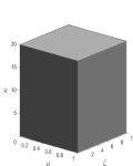
Figure 6: 90% S and qLL-S confidence sets for $\theta=(\rho,\kappa,\zeta)$ derived from the investment Euler equation model (7) using the sum of Gross Private Domestic Investment and Personal Consumption Expenditure on Durable Goods as investment proxy. A constant and $\Delta i_{t-1}$ are common instruments in all specifications while $u_{t-1}$ enters only in specifications (a) to (e) and (i) to (m). The additional instrument(s) by specification is (are): Baseline $r_{t-2}^{p}$; Mon. pol. shock: Romer and Romer’s (2004) monetary policy shock; Military news: Ramey and Zubairy’s (2018) military news shock; Oil: growth rate of real oil price; VXO: financial uncertainty.

In almost all cases, the results are very similar to Figure 4 that used only lagged variables as instruments. The specifications which include monetary policy shocks in the set of instruments for the SW investment measure, as shown in Figures 5 (b) and (f), result in a slight reduction of the S confidence sets. The reduction is somewhat more sizable for the specifications which include military news shocks in the set of instruments when using the JPT investment proxy. In Figures 6 (c) and (f) the resulting S sets are roughly 40% smaller than the rest of the S sets. Nevertheless even in this case, the parameters $\kappa$ and $\zeta$ remain very weakly identified. The main implication of using the military news shock is that values of $\rho>0.6$ can be rejected, which contradicts with the findings in SW and JPT. Therefore, contemporaneous information from arguably exogenous instruments does not seem to help identify the parameters of the investment equation. Additionally, as before, there is no evidence of parameter instability or violations of the moment conditions over subsamples.

5.3 Combining all the Instruments

The methods we have used so far exploited information arising from only a handful of instruments at a time, even though equation (7) implies a large number of potential instruments. This was done because the S and qLL-S sets become unreliable when the number of instrument is large relative to the sample size. With the sample sizes we are dealing with here, even a dozen instruments could make results unreliable. However, use of many instruments could potentially sharpen our inference if it happens to be the case that information is spread thinly over many instruments. To study this possibility, we compute split-sample S sets, which are robust to many weak instruments. Ideally, we would like to combine all the instruments that we have used so far in a single estimation, but because of data limitations with the external instruments, we do two separate estimations instead. The first uses four lags of the three instruments $\Delta i_{t},r_{t-1}^{p}$ and $u_{t}$, which are available over our full sample period. The second estimation adds to the aforementioned lagged instruments the external instruments that are available over a shorter sample. In both cases, we use approximately the first half of the sample to estimate the first-stage regression coefficients and the second half to compute the test statistic, as explained in Appendix B.2.

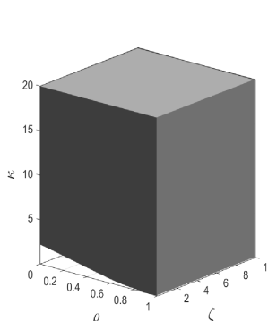
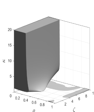
SW Investment JPT Investment 1968Q1-2019Q4 1968Q1-2019Q4 (a) (b) 4 lags         1970Q1-2007Q4 1970Q1-2007Q4 (c) (d) 4 lags + ext. instr.        

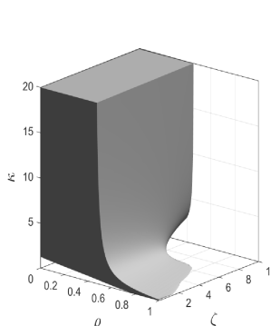
Figure 7: 90% Mikusheva split-sample S confidence sets for $\theta=(\rho,\kappa,\zeta)$ derived from the investment Euler equation model (7). Instruments - 4 lags: $\left\{\Delta i_{t-j},r_{t-1-j}^{p},u_{t-j}\right\}_{j=1}^{4}$. 4 lags + ext. inst.: additional instruments are Romer and Romer’s (2004) monetary policy shock; Ramey and Zubairy’s (2018) military news shock, the growth rate of real oil price, and the financial uncertainty (VXO). A constant is included in all specifications. The investment proxies are Fixed Private Investment (left column) and the sum of Gross Private Domestic Investment and Personal Consumption Expenditure on Durable Goods (right column). Newey and West (1987) HAC.

Figures 7 (a) and (b) report the results of the split-sample S confidence sets for $(\rho,\kappa,\zeta)$ with the lagged instruments only, using the SW and JPT investement data, respectively. The results with the SW data are essentially the same as before: very weak identification of all three parameters. The results with the JPT data are somewhat more informative than before. The size of the split-sample S confidence set is less than a third of the S and qLL-S sets reported in Figures 4(b) and (d). However, the confidence sets contain most of the values of $\kappa$ and $\zeta$, so most of the information gains affect only the parameter $\rho$: values greater than 0.5 are effectively excluded from the split-sample confidence set. This is consistent with the results reported in Figure 14 in Appendix D which compares the results using one and two lags of the instruments. The addition of more lags shrinks the JPT confidence sets but only in terms of $\rho$, and in the same direction as in Figure 7.

Figures 7 (c) and (d) perform the same exercise but adding the external instruments used in Figures 5 and 6, respectively. Note that the smaller sample size relative to Figures 7 (a) and (b) means that the results are not directly comparable - the combined larger instrument set can be more informative, but the smaller estimation sample makes inference less precise. Nevertheless, the pictures look very much in line with the results reported earlier. With SW investment data, the confidence set is entirely uninformative, exactly as in Figures 4 (a) and (c), and Figure 5 above. With JPT investment data, the split-sample S confidence set is about half the size of the sets in Figures 4 (b) and (d), with all the extra information affecting only the persistence parameter $\rho$. Interestingly, the confidence set in Figure 7 (d) is quite similar to the S set reported in Figure 6 (c) that uses military news as a single external instrument, suggesting that military news may be the most informative of all the instruments we have considered. Still, identification of $\kappa$ and $\zeta$ remains very weak. Therefore, we conclude that the previous uninformative confidence sets were not due to the use of a limited selection of the available instruments, and that the investment equation is genuinely weakly identified.

5.4 Semi-structural Model

Finally, to better understand why the structural parameters are so poorly identified beyond the weak instruments issues discussed above, we study a semi-structural model. Note that we can re-write (7) as

$$\left[1+\rho\left(\beta+\phi_{q}\right)\right]\Delta\widetilde{i}_{t}-\rho\Delta\widetilde{i}_{t-1}-\left[\beta+\phi_{q}+\rho\beta\phi_{q}\right]\Delta\widetilde{i}_{t+1}+\beta\phi_{q}\Delta\widetilde{i}_{t+2}$$

$$=\varphi\left(\widetilde{u}_{t+1}-\rho\widetilde{u}_{t}\right)-\phi\left(\widetilde{r}_{t}^{p}-\rho\widetilde{r}_{t-1}^{p}\right)+\epsilon_{t},$$ (8)

where $\varphi=\frac{\phi_{k}\zeta}{\kappa}$ and $\phi=\frac{1}{\kappa}$ are reduced-form parameters, for which we consider the ranges $[0,10]$ and $[0,20]$, respectively.

For ease of exposition, we construct two-dimensional confidence sets for $(\varphi,\phi)$ for fixed values of $\rho$ at 0.0, 0.6, 0.8, and 0.9. We estimate (8) using the same set of instruments and sample period as in Figure 4. Figure 8 plots the resulting two-dimensional confidence sets for $(\varphi,\phi)$.

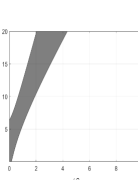
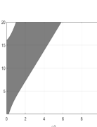
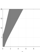
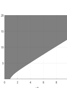
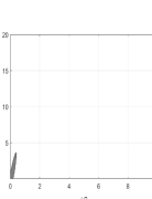
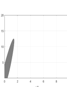
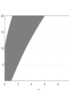
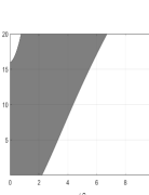
Panel A: SW Investment Proxy $\rho=0.0$ $\rho=0.6$ $\rho=0.8$ $\rho=0.9$ (a) (b) (c) (d) S sets          (e) (f) (g) (h) qLL-S sets         Panel B: JPT Investment Proxy $\rho=0.0$ $\rho=0.6$ $\rho=0.8$ $\rho=0.9$ (a) (b) (c) (d) S sets                (e) (f) (g) (h) qLL-S sets               

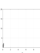
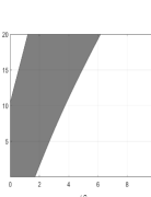
Figure 8: 90% S and qLL-S confidence sets for $(\varphi,\phi)$ derived from the investment Euler equation model (8) with Fixed Private Investment and the sum of Gross Private Domestic Investment and Personal Consumption Expenditure on Durable Goods as investment proxies (Panels A and B, respectively). Instruments: a constant, $\Delta i_{t-1}$, $r^{p}_{t-2}$ and $u_{t-1}$. Newey and West (1987) HAC. Period: 1967Q1-2019Q4.

The figure suggests that, when $\rho$ is between 0 and 0.6, $\varphi$ and $\phi$ are well-identified with their respective confidence intervals sitting tightly around 0. Looking at equation (8), this suggests limited responsiveness of investment growth to changes in capital utilization and the real interest rate. This implies that in addition to the weak identification issues discussed above, the mapping from reduced-form to structural parameters is also resulting in poorly identified confidence sets for the latter ones, even when the former ones are well-identified. For instance, despite $\phi$ being well identified when $\rho=0$ or $\rho=0.6$, its reciprocal $\kappa$ is not, since the confidence interval for $\phi$ includes 0. Similarly, even though both $\varphi$ and $\phi$ are well identified when the investment-specific shock is moderately persistent, the structural parameter $\zeta$ is not, since $\phi_{k}$ (which is calibrated in our earlier exercises) is very small, therefore resulting in poor identification of $\zeta$.

As for the sake of comparison, Table 2 shows the estimates of the well-identified reduced-form parameters $(\varphi,\phi)$ implied by the estimates of the elasticity of capital utilization cost $(\zeta)$ and the investment adjustment cost $(\kappa)$ in Figure 1. As explained above, because of the mapping from reduced-form to structural parameters, the large differences in the structural parameters does not translate into large differences in the reduced-form ones, whose implied values are consistent with our semi-structural estimation.

Table 2: Values of the reduced-form parameters $\phi$ and $\varphi$
implied by the estimates of $\kappa$ and $\zeta$ from Figure 1

	$\phi$	$\varphi$
CEE (2005)	0.40	0.0001
SW (2007)	[0.13-0.25]	[0.003-0.02]
JPT (2010)	[0.26-0.48]	[0.03-0.12]
ACEL (2011)	0.67	0.26
CTW (2011)	[0.05-0.10]	[0.0003-0.002]
CMR (2014)	0.09	0.008
AABC (2020)	[0.18-0.35]	[0.007-0.01]
IKR (2020)	[0.30-0.67]	[0.04-0.15]

• Notes: As in Figure 1, the labels refer to the following papers: Christiano et al. - CEE(2005), Smets and Wouters - SW(2007), Justiniano et al. - JPT(2010), Altig et al. - ACEL(2011), Christiano et al. - CTW(2011), Christiano et al. - CMR(2014), Arias et al. - AABC(2020), Inoue et al. - IKR(2020)

To understand why identification of the semi-structural parameters $\varphi$ and $\phi$ worsens for higher values of $\rho$, we look at the autocorrelations of $r_{t}^{p}$ and $u_{t+1}$. The first and second autocorrelations of $r_{t}^{p}$ in our baseline sample are 0.90 and 0.83 respectively, while the same autocorrelations for $u_{t+1}$ are 0.96 and 0.87, indicating that both series are highly persistent. Therefore, for small values of $\rho$, the instruments $r_{t-2}^{p}$ and $u_{t-1}$ are highly correlated with the endogenous variables of the system, resulting in better identification. In contrast, as the value of $\rho$ increases, $(u_{t+1}-\rho u_{t})$ and $(r_{t}^{p}-\rho r_{t-1}^{p})$ in equation (8) resemble white-noise processes, making lagged endogenous variables weak instruments. This is illustrated in Figure 9 which is a scatter plot of the fitted values of the endogenous regressors $(\phi_{k}u_{t+1}-\rho\phi_{k}u_{t})$ and $(r_{t}^{p}-\rho r_{t-1}^{p})$ from their respective first-stage regressions on the baseline set of instruments used to construct Figures 4 and 8. The left column, which plots the results for $\rho=0$, shows that the instruments are relatively strong as the fitted values mostly lie along the 45-degree line. In contrast, for high values of $\rho$, as in the right column which plots the results for $\rho=0.8$, the values of both $(\phi_{k}u_{t+1}-\rho\phi_{k}u_{t})$ and $(r_{t}^{p}-\rho r_{t-1}^{p})$ are tightly packed around zero and are uncorrelated with the fitted values from the first-stage regressions, suggesting that instruments are weak.

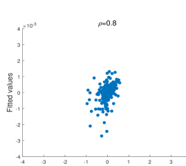
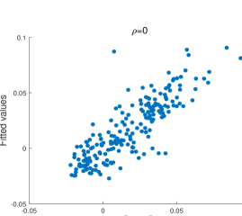
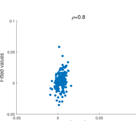
Figure 9: Scatter plot of the fitted values of the endogenous regressors $(\phi_{k}u_{t+1}-\rho\phi_{k}u_{t})$ and $(r_{t}^{p}-\rho r_{t-1}^{p})$ from their respective first-stage regressions on the baseline instruments for two different values of $\rho$.

6 Implications for DSGE Models

In this Section, we discuss the main implications of our analysis. In the Introduction, we argue about the importance of using the GMM methodology to assess the empirical fit in aggregate data of the investment equation commonly used in DSGE models. Our results support the investment equation, in the sense that there is no evidence against it. Moreover, we ask whether the GMM methodology could shed some light on the values of the parameters of this equation given the wide range found in the literature. Unfortunately, the answer is negative, because these parameters are weakly identified. This raises two questions to which we turn in the next two subsections. The first relates to the sensitivity of the DSGE results to changes in the three main parameters of interest: are any of these parameters relatively more important for the dynamic properties of a standard DSGE model, and thus relatively more important to pin down? Second, how do DSGE models attain identification of these parameters?

6.1 Sensitivity of DSGE Dynamics to the Parameters of the Investment Equation

Figures 10-11 mimic previous Figure 2. The figures show how the impulse responses of output and investment to the seven structural shocks in JPT’s model change when we allow the value of $\kappa$ and $\zeta$ to range in the 90% baseline S confidence set, while the remaining parameters are fixed at the posterior median of JPT, including $\rho$ which is set to 0.72. To highlight the relative sensitivity of the model dynamics to the values of $\kappa$ and $\zeta$, in both figures the dark shaded areas visualize all the possibilities when both $\kappa$ and $\zeta$ vary in the 90% S confidence set. In Figure 10, the light shaded areas depict all the possibilities when $\kappa$ ranges in its 90% S confidence set, while $\zeta$ is set to the JPT posterior median ($\zeta=5.30$), while, in Figure 11, the light shaded areas depict all the possibilities when $\zeta$ ranges in its 90% S confidence set, while $\kappa$ is set to the JPT posterior median ($\kappa=2.85$). Comparing the two figures, it is clear that the IRFs are very sensitive to the value of $\kappa,$ while they are little sensitive to the value of $\zeta.$ With the sole exception of the IRFs to a government spending shock (and marginally the wage markup shock), different values of $\zeta$ within the 90% S confidence set change the IRFs only slightly, while most of the variation is due to the different values of $\kappa.$ This is particularly true for the shock that directly impacts the investment equation, that is, the investment-specific shock, as well as for the other two shocks that in these models are usually found to be the other main drivers of business cycle fluctuations, that is, the technology shock and the preference shock.

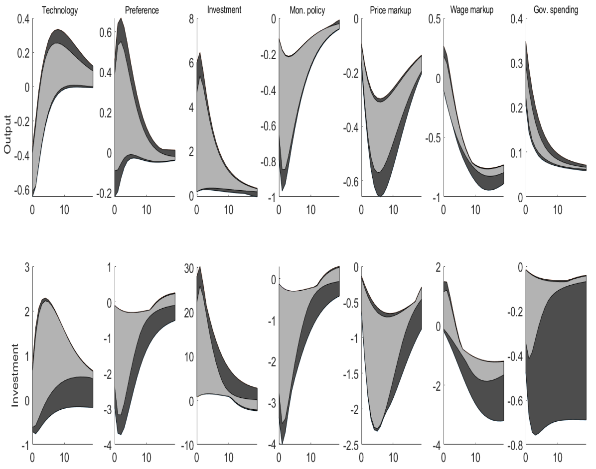
Figure 10: Impulse responses of output and investment to a one-standard deviation structural shock in JPT’s model evaluated at the posterior median estimate of all parameters except $\kappa$ and $\zeta$. Dark shaded areas: both $\kappa$ and $\zeta$ vary in the 90% S confidence set; light shaded areas: only $\kappa$ vary and $\zeta=5.30$ (posterior median estimate of JPT).

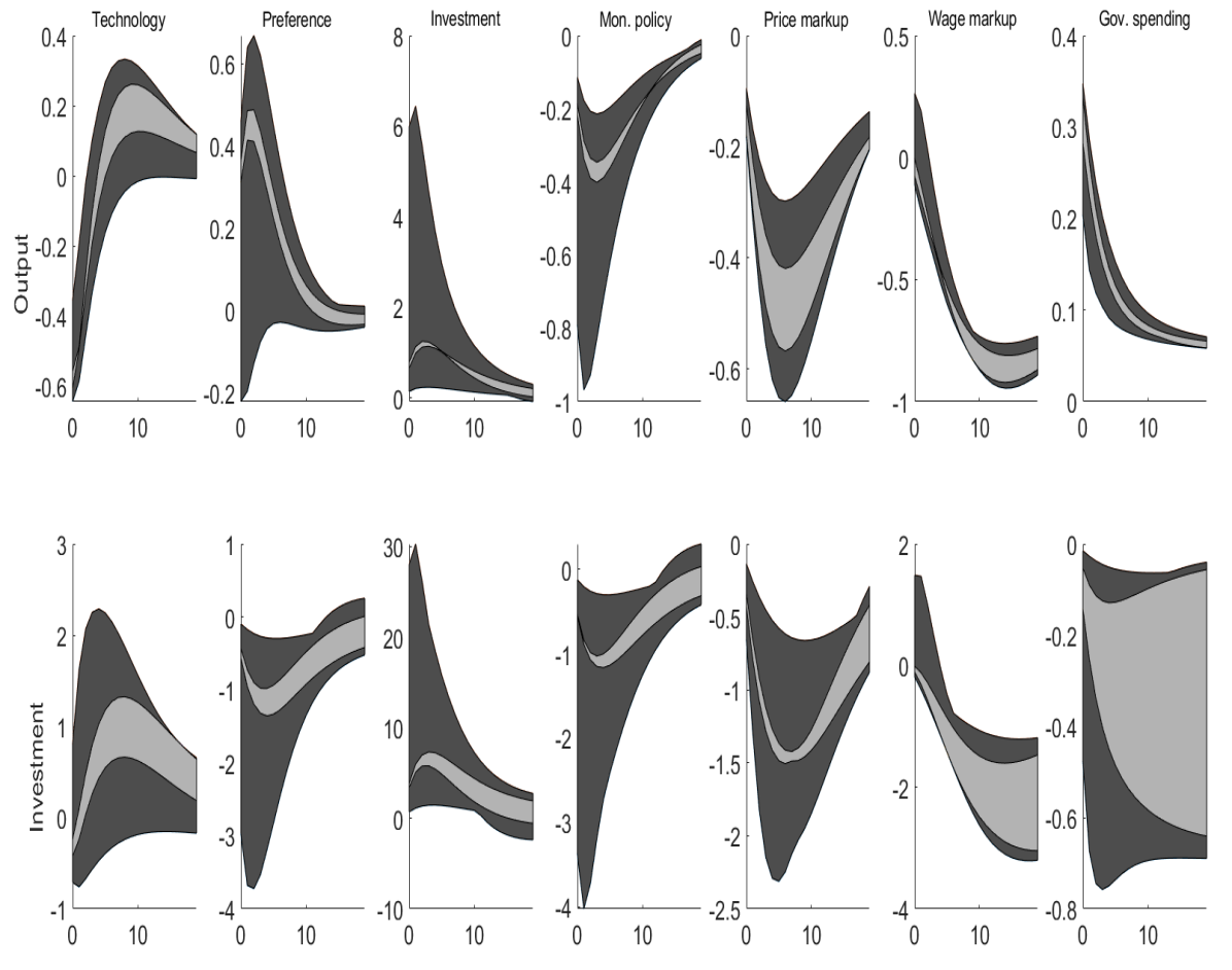
Figure 11: Impulse responses of output and investment to a one-standard deviation structural shock in JPT’s model evaluated at the posterior median estimate of all parameters except $\kappa$ and $\zeta$. Dark shaded areas: both $\kappa$ and $\zeta$ vary in the 90% S confidence set; light shaded areas: only $\zeta$ vary and $\kappa=2.85$ (posterior median estimate of JPT).

Figure 12 uncovers the same message by looking at the variance decomposition, similarly to Table 1. Figure 12 shows how the variance decomposition of output growth changes when $\kappa$ and $\zeta$ vary in the 90% baseline S confidence set, and, as before, the Figure displays the marginal effects of both $\kappa$ and $\zeta,$ obtained by varying each parameter at a time keeping the other fixed at the JPT posterior median. Even more striking than for the IRFs, almost all the variation in the variance decomposition is due to changes in the values of $\kappa,$ while the role of $\zeta$ is negligible.

Figure 12: Forecast error variance decomposition of output growth in JPT’s model evaluated at the posterior median estimate of all parameters except $\kappa$ and $\zeta$. Blue bars: both $\kappa$ and $\zeta$ vary in the 90% S confidence set; orange bars: only $\kappa$ vary and $\zeta=5.30$ (posterior median estimate of JPT); yellow bars: only $\zeta$ vary and $\kappa=2.85$ (posterior median estimate of JPT).

Together with Figure 3, these results suggest that $\kappa$ and $\rho$ are the key parameters that shape the dynamics of investment in a standard medium-scale DSGE model. The former defines the dynamic response of investment (and as a consequence of output) to the different shocks, and more prominently to the investment shock. A high value of the latter is fundamental to determine the persistent response of investment to the investment shock, and hence to replicate the persistent behaviour that characterizes the aggregate macroeconomic time series data. In contrast, $\zeta$ does not seem very relevant for determining the dynamic response of investment (and of output), so one could imagine that its value would be difficult to identify in the data. This is what we turn to next.

6.2 Identification of the Parameters of the Investment Equation in DSGE Models

In this Section we try to understand how DSGE models estimated with Bayesian methods obtain identification of the investment equation parameters, and compare this with our results. In comparison with our GMM single-equation approach, the DSGE system-based Bayesian estimation exhibits two main features that can help identification. The first is the use of priors in the Bayesian method. The second is the combination of the joint model dynamics of the variables in the system and the related cross-equation restrictions implied by rational expectations. We would like to distinguish the role of these two features. To this end, we perform the following exercise, displayed in Figure 13: Panel A. Let us look first at the top-left panel, regarding the parameter $\kappa$. As usually done in this type of models, the panel exhibits the difference between the prior (grey solid line) and the posterior (black solid line) to get a sense of how informative are the data. In addition, the panel features a third dashed line which is the posterior obtained by allowing the structural shocks of the model to be correlated in the estimation. The correlation among the shocks should ‘relax’ the ties implied by the cross-equation restrictions in the model. Thus, a comparison between the posteriors with and without shock correlations - i.e., between the solid line and the dashed line - should give a sense of how much the structure of the model helps in achieving identification. The bottom-left panel displays the same lines as the top left-panel, but assuming a looser prior. Hence, a comparison between the top-left and the bottom-left panel should instead highlight the role of the prior in helping identification. Columns two and three in Figure 13: Panel A show the same analysis for the parameters $\zeta$ and $\rho.$ Figure 13: Panel A shows this exercise using JPT’s model and data, while Figure 13: Panel B does the same for JPT’s model but with SW’s data.

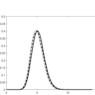
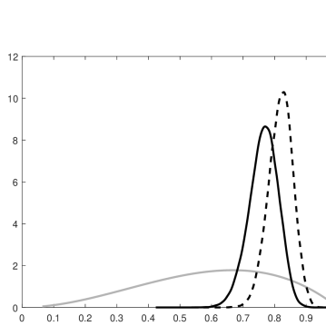
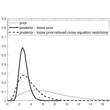
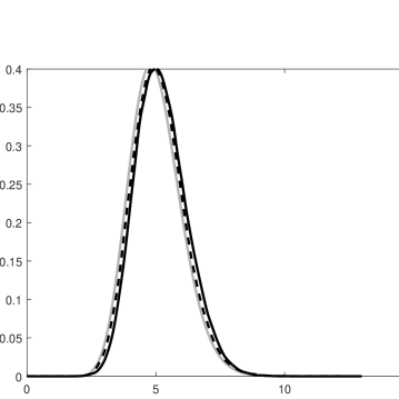
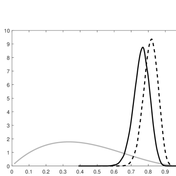
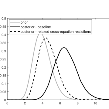
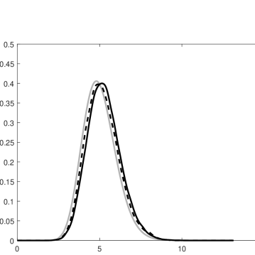
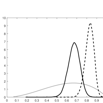
Panel A: JPT’s dataset Investment adjustment cost ($\kappa$) Elasticity capital utilization cost ($\zeta$) AR(1) coefficient investment shock ($\rho$) (a) (b) (c)     (d) (e) (f)     Panel B: SW’s dataset Investment adjustment cost ($\kappa$) Elasticity capital utilization cost ($\zeta$) AR(1) coefficient investment shock ($\rho$) (g) (h) (i)     (j) (k) (l)    

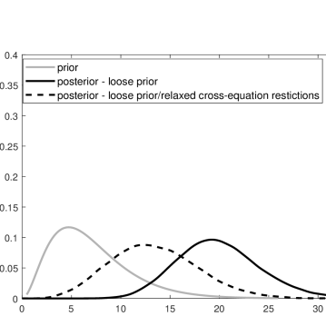
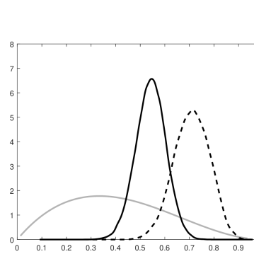
Figure 13: Prior-posterior plot: JPT’s model

Let us look at the implication of this analysis for the different parameters of interest. Regarding $\kappa$ (see the first column in Figure 13), the top-left panel in Figure 13: Panel A suggests that the cross-equation restrictions of the model do help in achieving identification because the dashed line is closer to the prior, while the solid line (where no correlations between the shocks are allowed) is instead much tighter. The bottom-left panel shows that the role of the prior in achieving identification is instead marginal because the posterior estimate is almost unchanged with a looser prior than in the top-left panel. However, the result is different if we estimate the same JPT model but with SW’s data, as shown in Figure 13: Panel B. While there is still an important role for cross-equation restrictions, the prior seems to be very important too, because the posterior in the bottom-left panel is much more dispersed than in the top-left one. Moreover, the SW’s data set implies a larger value, i.e. posterior mode, for $\kappa.$

Regarding $\zeta$ (see the second column in Figure 13), the results are very consistent with our GMM estimation: $\zeta$ is not identified by the data, and the identification is fully due to the prior for both data sets. Moreover, this is consistent with our analysis in the previous Section 6.1, where we show that changes in the value of $\zeta$ are not affecting much the dynamics of the model, thus possibly impairing identification.

Regarding $\rho$ (see the third column in Figure 13), the two Panels suggest that the data are quite informative and the parameter is very well identified. Both posteriors - with and without allowing for correlated shocks - move away distinctly from the prior and are quite peaked. The cross-equation restrictions call for a smaller value of this parameter, shifting the posterior towards the left, while SW’s data set implies a lower value for the parameter and a relatively less peaked posterior. The persistence parameter of the investment shock is thus well identified to be high, even if we relax the cross-equation restrictions and use a loose prior. We conjecture this to be due to the fact that the model wants to match the very persistent dynamics of the observable macroeconomic time series used in the Bayesian estimation. In contrast, our estimation procedure suggests that the investment equation is consistent with any value of $\rho,$ using fewer observables with respect to the system-based estimation. Interestingly, if anything, the GMM approach suggests a lower value of $\rho$, because, as noted earlier, with JPT’s data Figures 7 (b) and (d) and Figure 6 (c) shrinks the confidence set of $\rho$ to values roughly lower than 0.5. Moreover, in Section 5.4 we analyze the implications of different calibrations of $\rho$ for the identification of the reduced-form parameters in a semi-structural estimated equation, and we find that lower values of $\rho$ lead to sharper identification of the semi-structural parameters. If one wants to estimate $\rho$ more precisely from the data (e.g., from IRFs in DSGEs), one would need to make additional assumptions about the specification of the other variables that would allow us to identify the shock $\widetilde{\nu}_{t}$ in equation (6) and hence estimate its autocorrelation directly. We cannot do that in a limited information approach.

Our results point out that identification of the structural parameters in DSGE models could be achieved through cross-equation restrictions implied by the joint dynamics of the full system. On the other hand, these assumptions could potentially lead to biased estimates whenever some other parts of the system are misspecified, as we show next.

6.3 On Cross-equation Restrictions and Identification

In this Subsection, we use a simple example to demonstrate how cross-equation restrictions from a system method can achieve identification of a model that is not identified using a single-equation GMM approach at the cost of losing robustness to misspecification.

Recall that GMM estimates the single equation (6), where we have also assumed that $\beta$ and $\delta$ are known. For the purpose of this discussion it suffices to simplify the exposition to the case of a single unknown parameter. Hence, assume $\rho=0$ and $\kappa$ is known, so there is only one unknown parameter, $\zeta$, and the model in equation (6) can be written as

$$E_{t}y_{t+2}=\zeta E_{t}x_{t+1}+\widetilde{\nu}_{t}$$ (9)

where $y_{t+2}:=\kappa\left(\Delta\widetilde{i}_{t}-\left(\beta+\phi_{q}\right)\Delta\widetilde{i}_{t+1}+\beta\phi_{q}\Delta\widetilde{i}_{t+2}\right)+\widetilde{r}_{t}^{p}$ and $x_{t}:=\phi_{k}\widetilde{u}_{t}$, with $\phi_{k}=1-\left(1-\delta\right)\beta.$

Now, $\zeta$ is identified in (9) if and only if $var\left(E_{t}x_{t+1}\right)>0$. But in a limited-information setting, we do not observe $E_{t}x_{t+1},$ so we have to instrument for it using predetermined variables $Z_{t}$ that belong to the information set at time $t-1$. Specifically, the corresponding single-equation GMM regression for (9) is

$$y_{t+2}=\zeta x_{t+1}+\underbrace{\left[\widetilde{\nu}_{t}+y_{t+2}-E_{t}y_{t+2}-\zeta\left(x_{t+1}-E_{t}x_{t+1}\right)\right]}_{\xi_{t}},$$ (10)

with $E_{t-1}\xi_{t}=0,$ and any predetermined variable is a valid instrument for $x_{t+1}$. So, for the (single-equation) GMM approach to identify $\zeta$ it is necessary that $var\left(E_{t-1}x_{t+1}\right)>0$.

It is possible to come up with examples where a system method will identify $\zeta$ while the single-equation GMM approach will not. Suppose

$$x_{t}=\omega_{t}+\theta\omega_{t-1},\quad\left|\theta\right|<1,$$ (11)

(an invertible first-order moving average process) and $\omega_{t}$ (the structural shock driving capacity utilization $x_{t}=\phi_{k}\widetilde{u}_{t}$) is orthogonal to the investment-specific technology shock $\widetilde{\nu}_{t}$. Equation (11) implies that $E_{t}x_{t+1}=\theta\omega_{t}$, while $E_{t-1}x_{t+1}=0$. So, $\zeta$ can be identified if we use the additional equation (11), but it is not identified from a single-equation approach that does not make enough assumptions to pin down $E_{t}x_{t+1}$.

In terms of implementation, because of the triangular nature of this simple example, i.e., because (11) does not involve $\widetilde{\nu}_{t}$ or $y_{t}$, we can demonstrate how identification works as follows. First estimate (11) to obtain $\omega_{t}$ and $\theta$, next, compute $z_{t}:=\theta\omega_{t}=E_{t}x_{t+1}$, and finally, estimate $\zeta$ from the regression

$$y_{t+2}=\zeta z_{t}+\underbrace{\left(\widetilde{\nu}_{t}+y_{t+2}-E_{t}y_{t+2}\right)}_{e_{t}}\text{.}$$ (12)

Unless $\theta=0$ (rank condition), which would imply $z_{t}=0$ for all $t$, the above regression identifies $\zeta$, so a system analysis will produce bounded confidence sets, while the single-equation GMM analysis based on (9) that uses only predetermined variables to instrument for $x_{t+1}$ will produce unbounded confidence sets.

Misspecification

The increased precision of the system approach comes at the cost of lower robustness to misspecification. Suppose the true law of motion for $x_{t}$ were given by

$$x_{t}=\gamma x_{t-1}+\omega_{t},$$ (13)

i.e., an AR(1) instead of an MA(1). Using (11) instead of (13), one would get an inconsistent estimate of $E_{t}x_{t+1},$ say $z_{t}^{\ast}=\theta^{\ast}\omega_{t}^{\ast}$, where $\theta^{\ast},\omega_{t}^{\ast}$ are the pseudo-true values of $\theta,\omega_{t}$ in the MA(1) specification (11), when the data is generated according to (13), instead of the true $z_{t}=\gamma x_{t}$ from (13). So, instead of using (12), a misspecified system approach would be estimating $\zeta$ from the incorrect regression

$$y_{t+2}=\zeta z_{t}^{\ast}+\underbrace{\left[\zeta\left(z_{t}-z_{t}^{\ast}\right)+e_{t}\right]}_{e_{t}^{\ast}},\qquad cov(z_{t}^{*},e_{t}^{*})\neq 0,$$ (14)

which suffers from omitted variable bias because $z_{t}^{\ast}$ correlates with $e_{t}^{\ast},$ see Appendix F. Thus, the system estimate of $\zeta$ will be biased.

A DSGE model allows us to use cross-equation restrictions to determine $E_{t}x_{t+1}$ under rational expectations, see Footnote 3. In this present simple example, one may think that we are not actually using any cross-equation restrictions because $E_{t}x_{t+1}=\theta\omega_{t}$ does not involve the structural parameter $\zeta$ of the original target equation (9). However, in more general (e.g., non-triangular) settings where $x_{t}$ is allowed to be simultaneously determined with $y_{t}$, $E_{t}x_{t+1}$ will depend also on $\zeta$, and system estimation will indeed impose cross-equation restrictions.

7 Conclusions

We assess the empirical performance of the most commonly employed specification of investment behavior in modern operational DSGE models employed for policy analysis. The specification of the investment block of these models is based on the investment adjustment cost specification proposed by Christiano et al. (2005) together with variable capital utilization. We employ the same limited-information methodology that was used in the extant literature on the empirical performance of other key parts of DSGE models, such as the New Keynesian Phillips curve, the monetary policy rule, and the consumption Euler equation.

Our results are mixed. On the one hand, the investment equation is not rejected by the data. On the other hand, there is little information that aggregate data could provide to identify the key structural parameters of the investment block of current medium-scale DSGE models. Hence, this identification has to come from the cross-equation restrictions that other parts of the model imply. However, semi-structural estimation shows that investment is insensitive to changes in capital utilization and the real interest rate. In fact, the semi-structural parameters - the elasticity of investment to the real interest rate and capital utilization - are quite tightly estimated to be near zero when the persistence of the investment-specific shock is assumed to be low. Finally, similar to the results in Ascari et al. (2021), structural change is not as informative for the identification as it was found to be for the NKPC, and there is no evidence of parameter instability.

Finally, we investigate how DSGE models estimated with Bayesian methods obtain identification of the investment Euler equation parameters, in contrast to our methodology. Using the JPT model, we find that the investment adjustment cost parameter is mainly identified by the model cross-equation restrictions, while the role of the prior in achieving identification is marginal. The elasticity of capital utilization is not identified by the data. This is consistent with the evidence in JPT and with our analysis, which shows that changes in the value of $\zeta$ are not affecting much the dynamics of the model, thus possibly impairing identification. The data are quite informative, instead, on the persistence parameter of the investment-specific shock which is thus well identified to be high, even if we relax the cross-equation restrictions and use a loose prior. We conjecture this to be due to the fact that the model wants to match the very persistent dynamics of the observable macroeconomic time series used in the Bayesian estimation. In conclusion, our results suggest that identification of the structural parameters in DSGE models could be achieved through cross-equation restrictions implied by the joint dynamics of the full system. However, these assumptions could potentially lead to biased estimates whenever some other parts of the system are misspecified.

Appendix

Appendix A Derivation of equation (7)

The representative household chooses ${I_{t}}$, ${\hat{K}_{t+1}}$, ${B_{t+1}}$, and ${u_{t}}$ to maximise (1) under the period-by-period budget constraint (2) and capital accumulation equation (4). The first-order conditions are

$$I_{t}:\hskip 12.0pt1= \nu_{t}Q_{t}\left[1-\mathcal{S}\left(\dfrac{I_{t}}{I_{t-1}}\right)-\mathcal{S}^{\prime}\left(\dfrac{I_{t}}{I_{t-1}}\right)\left(\dfrac{I_{t}}{I_{t-1}}\right)\right]$$

$$+\beta E_{t}\left\{\dfrac{\lambda_{t+1}}{\lambda_{t}}\mathcal{S}^{\prime}\left(\dfrac{I_{t+1}}{I_{t}}\right)\left(\dfrac{I_{t+1}}{I_{t}}\right)^{2}\nu_{t+1}Q_{t+1}\right\},$$

$$\hat{K}_{t+1}:\hskip 12.0ptQ_{t}= \beta E_{t}\left\{\dfrac{\lambda_{t+1}}{\lambda_{t}}\left[r_{t+1}^{k}u_{t+1}-a(u_{t+1})+Q_{t+1}\left(1-\delta\right)\right]\right\},$$

$$B_{t+1}:\hskip 12.0pt1= \beta E_{t}\left\{\dfrac{\lambda_{t+1}}{\lambda_{t}}\dfrac{R_{t}}{\pi_{t+1}}\right\},\ \text{and}$$

$$u_{t}:\hskip 12.0ptr_{t}^{k}= a^{\prime}\left(u_{t}\right),$$

where $Q_{t}$ denotes the marginal $\mathcal{Q}$, defined as the ratio of the Lagrange multipliers associated with the capital accumulation equation and the budget constraint $\left(\lambda_{t}\right)$, and $\pi_{t+1}$ is the inflation rate in period $t+1$.

Log-linearizing the above first-order conditions around the non-stochastic steady state yields

$$\widetilde{q}_{t} =\kappa\left(\widetilde{i}_{t}-\widetilde{i}_{t-1}\right)-\beta\kappa\left(E_{t}\widetilde{i}_{t+1}-\widetilde{i}_{t}\right)-\widetilde{\nu}_{t},$$ (15)

$$\widetilde{q}_{t} =E_{t}\widetilde{\lambda}_{t+1}-\widetilde{\lambda}_{t}+\beta\bar{r}^{k}E_{t}\widetilde{r}_{t+1}^{k}+\beta\left(1-\delta\right)E_{t}\widetilde{q}_{t+1},$$ (16)

$$E_{t}\widetilde{\lambda}_{t+1}-\widetilde{\lambda}_{t} =-(\widetilde{r}_{t}-E_{t}\widetilde{\pi}_{t+1}),\ \text{and}$$ (17)

$$\widetilde{r}_{t}^{k} =\zeta\widetilde{u}_{t},$$ (18)

where lowercase letters with a tilde denote the respective log deviations of the variables from their steady state. Although (15)-(18) can be estimated, the empirical literature has struggled to find an appropriate proxy for $\tilde{q}_{t}$, the marginal $\mathcal{Q}$, which is unobservable. Hayashi (1982) showed that under some regularity conditions the average $\mathcal{Q}$ is equivalent to marginal $\mathcal{Q}$. However, subsequent empirical studies have confirmed such regularity conditions to be unsatisfactory, finding insignificant coefficients on average $\mathcal{Q}$. Thus, we follow the treatment in Groth and Khan (2010) and get rid of $\tilde{q}_{t}$ from the log-linearized conditions. Substituting (15) and (17) into (16) yields our preferred baseline investment Euler equation with IAC

$$\widetilde{i}_{t}= \dfrac{1/\kappa}{1+\beta+\phi_{q}}\left[\phi_{k}E_{t}\widetilde{r}_{t+1}^{k}-E_{t}\widetilde{r}_{t}^{p}+\widetilde{\nu}_{t}\right]$$

$$+\dfrac{1}{1+\beta+\phi_{q}}\widetilde{i}_{t-1}+\dfrac{\beta+\phi_{q}(1+\beta)}{1+\beta+\phi_{q}}E_{t}\widetilde{i}_{t+1}-\dfrac{\beta\phi_{q}}{1+\beta+\phi_{q}}E_{t}\widetilde{i}_{t+2}-\dfrac{\phi_{q}/\kappa}{1+\beta+\phi_{q}}E_{t}\widetilde{\nu}_{t+1},$$ (19)

where $\widetilde{r}_{t}^{p}$ denotes the log-deviation of ex-ante real interest rate from steady state, i.e., $\widetilde{r}_{t}^{p}=\widetilde{r}_{t}-\widetilde{\pi}_{t+1}$, and $\phi_{q}=(1-\delta)/(1-\delta+\bar{r}^{k})$; $\phi_{k}=\bar{r}^{k}/(1-\delta+\bar{r}^{k})$; and $\bar{r}^{k}=1/\beta-1+\delta$.

We can use (18) to substitute out the rental rate of capital, $\widetilde{r}_{t}^{k}$, which is an unobservable variable, with the capacity utilization, $\widetilde{u}_{t}$, for which a time series is available. So, (19) becomes

$$\widetilde{i}_{t}= \dfrac{1/\kappa}{1+\beta+\phi_{q}}\left[\phi_{k}\zeta E_{t}\widetilde{u}_{t+1}-E_{t}\widetilde{r}_{t}^{p}+\widetilde{\nu}_{t}\right]$$

$$+\dfrac{1}{1+\beta+\phi_{q}}\widetilde{i}_{t-1}+\dfrac{\beta+\phi_{q}(1+\beta)}{1+\beta+\phi_{q}}E_{t}\widetilde{i}_{t+1}-\dfrac{\beta\phi_{q}}{1+\beta+\phi_{q}}E_{t}\widetilde{i}_{t+2}-\dfrac{\phi_{q}/\kappa}{1+\beta+\phi_{q}}E_{t}\widetilde{\nu}_{t+1}.$$

Note that this equation is the same as equation (6) in the main text, that is simply rewritten in first differences of the investment terms. For any variable $x_{t}$ the rational expectations (RE) forecast error is $\eta_{t|t-1}^{x}=x_{t}-E_{t-1}(x_{t})$, which implies that $E_{t}(x_{t+1})=x_{t+1}-\eta_{t+1|t}^{x}.$ Moreover, $E_{t}\widetilde{\nu}_{t+1}=\rho\widetilde{\nu}_{t}$, since $\widetilde{\nu}_{t}\sim AR(1):\widetilde{\nu}_{t}=\rho\widetilde{\nu}_{t-1}+\varepsilon_{t}^{v}.$ Finally, define $E_{t}(\widetilde{i}_{t+2})=\widetilde{i}_{t+2}-\eta_{t+2|t}^{i}$, then

$$\widetilde{i}_{t}= \dfrac{1/\kappa}{1+\beta+\phi_{q}}\left[\phi_{k}\zeta\widetilde{u}_{t+1}-\phi_{k}\zeta\eta_{t+1|t}^{u}-\widetilde{r}_{t}^{p}+\eta_{t+1|t}^{\pi}\right]+\dfrac{1}{1+\beta+\phi_{q}}\widetilde{i}_{t-1}$$

$$+\dfrac{\beta+\phi_{q}(1+\beta)}{1+\beta+\phi_{q}}\left(\widetilde{i}_{t+1}-\eta_{t+1|t}^{i}\right)-\dfrac{\beta\phi_{q}}{1+\beta+\phi_{q}}\left(\widetilde{i}_{t+2}-\eta_{t+2|t}^{i}\right)+\dfrac{1/\kappa\left(1-\phi_{q}\rho\right)}{1+\beta+\phi_{q}}\widetilde{\nu}_{t}\text{,}$$

or

$$\widetilde{i}_{t}= \dfrac{1/\kappa}{1+\beta+\phi_{q}}\left[\phi_{k}\zeta\widetilde{u}_{t+1}-\widetilde{r}_{t}^{p}\right]+\dfrac{1}{1+\beta+\phi_{q}}\widetilde{i}_{t-1}+\dfrac{\beta+\phi_{q}(1+\beta)}{1+\beta+\phi_{q}}\widetilde{i}_{t+1}$$

$$-\dfrac{\beta\phi_{q}}{1+\beta+\phi_{q}}\widetilde{i}_{t+2}+\varepsilon_{t},$$ (20)

where $\varepsilon_{t}=\tfrac{1/\kappa}{1+\beta+\phi_{q}}\left[-\phi_{k}\zeta\eta_{t+1|t}^{u}+\eta_{t+1|t}^{\pi}\right]-\tfrac{\beta+\phi_{q}(1+\beta)}{1+\beta+\phi_{q}}\eta_{t+1|t}^{i}+\tfrac{\beta\phi_{q}}{1+\beta+\phi_{q}}\eta_{t+2|t}^{i}+\tfrac{1/\kappa\left(1-\phi_{q}\rho\right)}{1+\beta+\phi_{q}}\widetilde{\nu}_{t}\text{.}$

Using the facts that $\widetilde{i}_{t}=\tfrac{1}{1+\beta+\phi_{q}}\widetilde{i}_{t}+\tfrac{\beta+\phi_{q}}{1+\beta+\phi_{q}}\widetilde{i}_{t}$, and $\tfrac{\beta+\phi_{q}(1+\beta)}{1+\beta+\phi_{q}}\widetilde{i}_{t+1}=\tfrac{\beta+\phi_{q}}{1+\beta+\phi_{q}}\widetilde{i}_{t+1}+\tfrac{\beta\phi_{q}}{1+\beta+\phi_{q}}\widetilde{i}_{t+1},$ the terms in $\widetilde{i}$ could be written as first difference, so equation (20) becomes

$$\dfrac{1}{1+\beta+\phi_{q}}\Delta\widetilde{i}_{t}=\dfrac{1/\kappa}{1+\beta+\phi_{q}}\left[\phi_{k}\zeta\widetilde{u}_{t+1}-\widetilde{r}_{t}^{p}\right]+\dfrac{\beta+\phi_{q}}{1+\beta+\phi_{q}}\Delta\widetilde{i}_{t+1}-\dfrac{\beta\phi_{q}}{1+\beta+\phi_{q}}\Delta\widetilde{i}_{t+2}+\varepsilon_{t}\text{,}$$

or

$$\Delta\widetilde{i}_{t}=\dfrac{\phi_{k}}{\kappa}\zeta\widetilde{u}_{t+1}-\dfrac{1}{\kappa}\widetilde{r}_{t}^{p}+\left(\beta+\phi_{q}\right)\Delta\widetilde{i}_{t+1}-\beta\phi_{q}\Delta\widetilde{i}_{t+2}+\left(1+\beta+\phi_{q}\right)\varepsilon_{t}\text{.}$$ (21)

We then just eliminate $\widetilde{\nu}_{t}$ in the error term $\varepsilon_{t}$, again by lagging (21), multiplying it by $\rho$, which results in

$$\rho\Delta\widetilde{i}_{t-1}=\dfrac{\rho\phi_{k}}{\kappa}\zeta\widetilde{u}_{t}-\dfrac{\rho}{\kappa}\widetilde{r}_{t-1}^{p}+\rho\left(\beta+\phi_{q}\right)\Delta\widetilde{i}_{t}-\rho\beta\phi_{q}\Delta\widetilde{i}_{t+1}+\rho\left(1+\beta+\phi_{q}\right)\varepsilon_{t-1}\text{,}$$

and subtracting the result from (21), such that

$$\Delta\widetilde{i}_{t}-\rho\Delta\widetilde{i}_{t-1}= \ \dfrac{\phi_{k}}{\kappa}\zeta\left(\widetilde{u}_{t+1}-\rho\widetilde{u}_{t}\right)-\dfrac{1}{\kappa}\left(\widetilde{r}_{t}^{p}-\rho\widetilde{r}_{t-1}^{p}\right)+\left(\beta+\phi_{q}\right)\left(\Delta\widetilde{i}_{t+1}-\rho\Delta\widetilde{i}_{t}\right)$$

$$-\beta\phi_{q}\left(\Delta\widetilde{i}_{t+2}-\rho\Delta\widetilde{i}_{t+1}\right)+\left(1+\beta+\phi_{q}\right)\left(\varepsilon_{t}-\rho\varepsilon_{t-1}\right)\text{.}$$

Rearranging terms we obtain the baseline specification (7)

$$\left[1+\rho\left(\beta+\phi_{q}\right)\right]\Delta\widetilde{i}_{t}= \ \rho\Delta\widetilde{i}_{t-1}+\left(\beta+\phi_{q}+\rho\beta\phi_{q}\right)\Delta\widetilde{i}_{t+1}-\beta\phi_{q}\Delta\widetilde{i}_{t+2}$$

$$+\dfrac{\phi_{k}}{\kappa}\zeta\widetilde{u}_{t+1}-\dfrac{\rho\phi_{k}}{\kappa}\zeta\widetilde{u}_{t}-\dfrac{1}{\kappa}\widetilde{r}_{t}^{p}+\dfrac{\rho}{\kappa}\widetilde{r}_{t-1}^{p}+\epsilon_{t}\text{,}$$

where

$$\epsilon_{t}:=\left(1+\beta+\phi_{q}\right)\left(\varepsilon_{t}-\rho\varepsilon_{t-1}\right)\text{,}$$ (22)

$\left(\varepsilon_{t}-\rho\varepsilon_{t-1}\right)=\tfrac{1/\kappa}{1+\beta+\phi_{q}}\left[-\phi_{k}\eta_{t+1|t}^{u}+\eta_{t+1|t}^{\pi}-\rho\left(-\phi_{k}\eta_{t|t-1}^{u}+\eta_{t|t-1}^{\pi}\right)\right]-\tfrac{\beta+\phi_{q}(1+\beta)}{1+\beta+\phi_{q}}\left(\eta_{t+1|t}^{i}-\rho\eta_{t|t-1}^{i}\right)$
$+\tfrac{\beta\phi_{q}}{1+\beta+\phi_{q}}\left(\eta_{t+2|t}^{i}-\rho\eta_{t+1|t}^{i}\right)+\tfrac{1/\kappa\left(1-\phi_{q}\rho\right)}{1+\beta+\phi_{q}}\varepsilon_{t}^{v}$, and $\varepsilon_{t}^{v}=\widetilde{\nu}_{t}-\rho\widetilde{\nu}_{t-1}$.

Appendix B Computational Details

The empirical moments of the linear model can be represented by $\frac{1}{T}\sum_{t=1}^{T}f_{t}\left(\theta,d\right)$, where $f_{t}\left(\theta,d\right)=Z_{t}^{\prime}\left(Y_{t}b\left(\theta\right)-X_{t}d\right)$, $Y_{t}=\left[\begin{array}[c]{cccccccc}\Delta\widetilde{i}_{t}&\Delta\widetilde{i}_{t-1}&\Delta\widetilde{i}_{t+1}&\Delta\widetilde{i}_{t+2}&\widetilde{r}_{t}^{p}&\widetilde{r}_{t-1}^{p}&\widetilde{u}_{t}&\widetilde{u}_{t+1}\end{array}\right]$, $Z_{t}=(X_{t},Z_{2,t})$ is the set of instrumental variables partitioned into included ($X_{t}$) and excluded ($Z_{2,t}$) instruments, $b\left(\theta\right)^{\prime}=\left[1+\rho\left(\beta+\phi_{q}\right),-\rho,-\left(\beta+\phi_{q}+\rho\beta\phi_{q}\right),\beta\phi_{q},\dfrac{1}{\kappa},-\dfrac{\rho}{\kappa},\phi_{k}\frac{\rho\zeta}{\kappa},-\phi_{k}\frac{\zeta}{\kappa}\right]^{\prime}$ is a vector which contains the structural parameters and $d$ are the strongly identified parameters, which are estimated before the computation of the statistical tests. The variable $X_{t}$ is $1$ corresponding to the constant in the estimated regression specification, which captures all the steady-state terms. We use $Z_{2,t}=\left\{\Delta i_{t-1},r_{t-2}^{p},u_{t-1}\right\}$ in our baseline results. The sample size is $T$.

B.1 S and qLL-S tests

Under $H_{0}:\theta=\theta_{0}$, $b\left(\theta_{0}\right)$ is fixed. The S statistic is

$$S\left(\theta_{0}\right)=\;\underset{d}{\min}\frac{1}{T}\sum_{t=1}^{T}f_{t}\left(\theta_{0},d\right)^{\prime}\widehat{V}\left(\theta_{0},d\right)^{-1}\sum_{t=1}^{T}f_{t}\left(\theta_{0},d\right).$$ (23)

The minimand in the above expression is the so-called continuously updated GMM objective function, evaluated at the continuously updated estimator for the untested parameter $d$ under $H_{0}$, see Stock and Wright (2000). The variance estimator $\widehat{V}\left(\theta_{0},d\right)$ is a heteroskedasticity and autocorrelation consistent (HAC) estimator of $\operatorname*{Var}\left(\frac{1}{\sqrt{T}}\sum_{t=1}^{T}f_{t}\left(\theta_{0},d\right)\right)$

$$\widehat{V}=\widehat{\Gamma}_{0}+\sum_{j=1}^{T}\omega_{j}\left(\widehat{\Gamma}_{j}+\widehat{\Gamma}_{j}^{\prime}\right)\text{,}$$

where $\widehat{\Gamma}_{j}=\left[\frac{1}{T}\sum_{t=j+1}^{T}\widehat{w}_{t}\widehat{w}_{t}^{\prime}\right]$, $\widehat{w}_{t}$ is  $f_{t}\left(\theta_{0},\hat{d}\right)-\bar{f}_{T}\left(\theta_{0},\hat{d}\right)$, $\bar{f}_{T}\left(\theta_{0},\hat{d}\right)=\frac{1}{T}\sum_{t=1}^{T}f_{t}\left(\theta_{0},\hat{d}\right)$. The parameter $\omega_{j}$ represents the Barlett kernel.

The S statistic is obtained by plugging $\hat{d}\left(\theta_{0}\right)$ into the objective function (23). The S test at level $\alpha$ rejects $H_{0}:\theta=\theta_{0}$ when the S statistic exceeds the $1-\alpha$ quantile of the $\chi^{2}$ distribution with $k_{z}-k_{x}$ degrees of freedom, where $k_{z}$ and $k_{x}$ are the number of elements in vectors $Z_{t}$ and $X_{t}$, respectively.

The qLL-S test rejects for large values of the statistic

$$\text{qLL--S}(\theta_{0})=\frac{10}{11}\text{S}\left(\theta_{0}\right)+\text{qLL--S}^{B}(\theta_{0})$$

where S$\left(\theta_{0}\right)$ is the S statistic evaluated at $\theta=\theta_{0}$, and qLL–S${}^{B}(\theta_{0})$ is the statistic that detects violations of the moment conditions in subsamples. The algorithm for computing the qLL–S^B is detailed in Magnusson and Mavroeidis (2014), where one can also find tables of critical values.

The confidence sets derived from the tests are obtained by performing a grid search over the parameter space. The 90% confidence sets are formed by the collection of points that do not reject $H_{0}:\theta=\theta_{0}$ at 10% significance level.

B.2 Split-sample S test

We derive a GMM version of the split-sample Anderson-Rubin test proposed by Mikusheva (2021) for linear models. Let $\bar{Y}_{t}$ be the demeaned values of $Y_{t}$. Define $\bar{W}_{t}\left(\theta\right)=\bar{Y}_{t}\frac{\partial b\left(\theta\right)}{\partial\theta^{\prime}}$, which is of dimension $1\times 3$, and let $\mathbf{W}\left(\theta\right)$ be the $T\times 3$ matrix with stacked terms $\bar{W}_{t}\left(\theta\right)$, $t=1,\ldots,T$.  Define also the matrices $\mathbf{Y}$ and $\mathbf{Z}$ of dimensions $T\times 8$ and $T\times k$ ($k=3$ in the baseline case) of stacked elements of $\bar{Y}_{t}$ and demeaned excluded instruments $\bar{Z}_{2,t}$. Partition $\mathbf{W}\left(\theta\right)=\mathbf{Y}\frac{\partial b\left(\theta\right)}{\partial\theta^{\prime}}$, $\mathbf{Y}$ and $\mathbf{Z}$ as $\mathbf{W}\left(\theta\right)=\left[\mathbf{W}_{1}\left(\theta\right):\mathbf{W}_{p}\left(\theta\right):\mathbf{W}_{2}\left(\theta\right)\right]$, $\mathbf{Y}=\left[\mathbf{Y}_{1}:\mathbf{Y}_{p}:\mathbf{Y}_{2}\right]$, and $\mathbf{Z}=\left[\mathbf{Z}_{1}:\mathbf{Z}_{p}:\mathbf{Z}_{2}\right]$.

In our case, the first subsample corresponds to 45% of the initial observations. The terms $\mathbf{W}_{p}\left(\theta\right)$ and $\mathbf{Z}_{p}$ are not used in the procedure in order to keep the exogeneity assumption valid. Following Mikusheva (2021, p. 30), we set $p=3$ because the error $\epsilon_{t}$ in (22) is adapted to the $t+2$ information set and the instruments include variables dated $t-1$. Then, estimate the fitted value of $\mathbf{W}_{2}\left(\theta\right)$ as $\mathbf{\hat{W}}_{2}\left(\theta\right)=\mathbf{Z}_{2}\hat{\pi}_{1}\left(\theta\right)$, where $\hat{\pi}_{1}\left(\theta\right)=\left(\mathbf{Z}_{1}^{\prime}\mathbf{Z}_{1}\right)^{-1}\mathbf{Z}_{1}^{\prime}\mathbf{W}_{1}\left(\theta\right)$ and $\mathbf{W}_{1}\left(\theta\right)=\mathbf{Y}_{1}\tfrac{\partial b\left(\theta\right)}{\partial\theta^{\prime}}.$

Finally, we compute the split-sample S statistic as

$$S_{M}(\theta)=\frac{1}{T_{2}}b\left(\theta\right)^{\prime}\mathbf{Y}_{2}^{\prime}\mathbf{\hat{W}}_{2}\left(\theta\right)\left[\widehat{\Omega}\left(\theta\right)\right]^{-1}\mathbf{\hat{W}}_{2}\left(\theta\right)^{\prime}\mathbf{Y}_{2}b\left(\theta\right),$$

where $\widehat{\Omega}\left(\theta\right)$ is the HAC estimator of the variance of $\frac{1}{\sqrt{T_{2}}}\sum_{t=t_{2}}^{T}\hat{\bar{W}}_{t}\left(\theta\right)^{\prime}\bar{Y}_{t}b\left(\theta\right)$ and $T_{2}$ corresponds to the number of observations of the last subsample.

The split-sample S test at level $\alpha$ rejects $H_{0}:\theta=\theta_{0}$ when $S_{M}(\theta_{0})$ exceeds the $1-\alpha$ quantile of a $\chi^{2}$ distribution with 3 degrees of freedom.

Appendix C Data

C.1 Data Sources for baseline analysis

• Gross Private Domestic Investment [GPDI]: Billions of Dollars, Seasonally Adjusted Annual Rate; Source: U.S. Bureau of Economic Analysis; FRED - https://fred.stlouisfed.org/series/GPDI.

• Fixed Private Investment [FPI]: Billions of Dollars, Seasonally Adjusted Annual Rate; Source: U.S. Bureau of Economic Analysis; FRED - https://fred.stlouisfed.org/series/FPI.

• Personal Consumption Expenditures: Durable Goods [PCDG]: Billions of Dollars, Seasonally Adjusted Annual Rate; Source: U.S. Bureau of Economic Analysis; FRED - https://fred.stlouisfed.org/series/PCDG.

• Gross Domestic Product (implicit price deflator) [GDPDEF]: Index 2012=100, Seasonally Adjusted; Source: U.S. Bureau of Economic Analysis; FRED - https://fred.stlouisfed.org/series/GDPDEF.

• Gross Private Domestic Investment (implicit price deflator) [A006RD3Q086SBEA]: Index 2012=100, Seasonally Adjusted; Source: U.S. Bureau of Economic Analysis; FRED - https://fred.stlouisfed.org/series/A006RD3Q086SBEA.

• Gross Private Domestic Investment: Fixed Investment (implicit price deflator) [A007RD3Q086SBEA]: Index 2012=100, Seasonally Adjusted; Source: U.S. Bureau of Economic Analysis; FRED -
  https://fred.stlouisfed.org/series/A007RD3Q086SBEA#0.

• Personal Consumption Expenditures: Durable goods (implicit price deflator) [DDURRD3Q086SBEA]: Index 2012=100, Seasonally Adjusted; Source: U.S. Bureau of Economic Analysis; FRED -
  https://fred.stlouisfed.org/series/DDURRD3Q086SBEA.

• Effective Federal Funds Rate [FEDFUNDS]: Percent, Not Seasonally Adjusted; Source: Board of Governors of the Federal Reserve System; FRED - https://fred.stlouisfed.org/series/FEDFUNDS.

• Capacity Utilization: Total Index [TCU]: Percent of Capacity, Seasonally Adjusted; Source: Board of Governors of the Federal Reserve System; FRED - https://fred.stlouisfed.org/series/TCU#0.

C.2 Additional exogenous instruments

• Romer and Romer (2004)’s narrative-based monetary policy shock (1969m3-2007m12); retrieved from Valerie A. Ramey’s website under Data and Programs for “Macroeconomic Shocks and Their Propagation”, 2016 Handbook of Macroeconomics. - https://econweb.ucsd.edu/~vramey/research.html#data.

• Ramey and Zubairy (2018)’s military news shock (1967q1-2015q4); retrieved from Valerie A. Ramey’s website under Programs and Data for “Government Spending Multipliers in Good Times and in Bad” with Sarah Zubairy, April 2018 Journal of Political Economy. - https://econweb.ucsd.edu/~vramey/research.html#data.

• Spot Crude Oil Price: West Texas Intermediate (WTI) [WTISPLC] (1967q1-2019q4); Deflated using CPI, Not Seasonally Adjusted; Source: Federal Reserve Bank of St. Louis; FRED - https://fred.stlouisfed.org/series/WTISPLC.

• VXO (1967q1-2019q4); Source: Chicago Board of Options Exchange (CBOE) and retrieved from FRED - https://fred.stlouisfed.org/series/VXOCLS.
  Note: This index is unavailable before 1986. Following Bloom (2009), pre-1986 monthly return volatilities are computed as the monthly standard deviation of the daily S&P500 index normalized to the same mean and variance as the VXO index when they overlap from 1986 onward.

C.3 Data Transformation

Investment: Investment series is first divided by the civilian non-institutional population (16 years or over) to convert into per capita terms and the resulting per capita series is then deflated using the respective implicit price deflators. Two per capita measures of investment are used in the analysis. They are:

1. SW - Real Fixed Private Investment (FPI).

2. JPT - sum of Real Gross Private Domestic Investment (GPDI) and Real Personal Consumption Expenditure: Durables Goods (PCDG).

The investment measures are computed, respectively, as $\tfrac{FPI}{P_{fpi}}\quad\text{and}\quad\tfrac{GDPI}{P_{gpdi}}+\frac{PCDG}{P_{pcdg}}$, where $P_{gpdi}$, $P_{pcdg}$ and $P_{fpi}$ are the respective implicit price deflators. Growth rates of investment are then computed as the log difference of the resulting series.

Inflation: Log difference of the quarterly implicit GDP price deflator.

Real (ex-post) interest rate: Difference between the Federal Funds Rate and the GDP deflator inflation rate.

Capacity utilization: Log of the capacity utilization index.

Narrative-based monetary policy shock: Quarterly average of the monthly series from Romer and Romer (2004).

Narrative-based military news shock: Defense news variable of Ramey (2016) scaled by trend GDP following Ramey and Zubairy (2018).

VXO: Quarterly average of the monthly series, demeaned and standardized.

Oil: Log difference of the real oil price series.

Appendix D Robustness checks

In this section we report further results to investigate the robustness of the empirical results reported in the main text. Figure 14 shows the results when we use two lags of endogenous variables as instruments and compares them with our baseline results using one lag. Figure 15 shows the results when we restrict our estimation sample to 2004Q4 (as in SW and JPT) and compares it with our baseline sample ending in 2019Q4. Figures 16 and 17 correspond to Figures 5 and 6 in the main text, respectively, but the external instruments are now added together with $r_{t-2}^{p}$ and ${u}_{t-1}$ in the set of instruments. The results are unchanged when using external instruments both for the SW and JPT investment measures, respectively. The main conclusion from these sensitivity analyses is that the results reported in the paper remain largely robust.

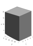
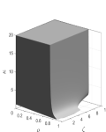
SW Investment JPT Investment One Lag Two Lags One Lag Two Lags (a) (b) (c) (d) S sets       (e) (f) (g) (h) qLL-S set      

Figure 14: 90% S and qLL-S confidence sets for $\theta=(\rho,\kappa,\zeta)$ in the investment euler equation model (7). Instruments: One lag - constant, $\Delta i_{t-1}$, $r^{p}_{t-2}$, $u_{t-1}$; Two lags - constant, $\Delta i_{t-1}$, $\Delta i_{t-2}$, $r^{p}_{t-2}$, $r^{p}_{t-3}$, $u_{t-1}$, $u_{t-2}$. Left two columns show the results based on using Fixed Private Investment as investment proxy, while right two columns use the sum of Gross Private Domestic Investment and Personal Consumption Expenditure on Durable Goods as investment proxy. Period: 1967Q1-2019Q4. Newey and West (1987) HAC.

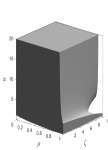
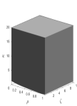
SW Investment JPT Investment 1967Q1-2004Q4 1967Q1-2019Q4 1967Q1-2004Q4 1967Q1-2019Q4 (a) (b) (c) (d) S sets       (e) (f) (g) (h) qLL-S set      

Figure 15: 90% S and qLL-S confidence sets for $\theta=(\rho,\kappa,\zeta)$ in the investment euler equation model (7). Instruments: constant, $\Delta i_{t-1}$, $r^{p}_{t-2}$, $u_{t-1}$. Left two columns show the results based on using Fixed Private Investment as investment proxy, while right two columns use the sum of Gross Private Domestic Investment and Personal Consumption Expenditure on Durable Goods as investment proxy. Newey and West (1987) HAC.

Exogenous Instruments with SW Investment Proxy Baseline Mon. pol. shock Military news Oil 1967Q1-2019Q4 1969Q2-2007Q4 1967Q1-2015Q4 1967Q1-2019Q4 (a) (b) (c) (d) S sets       VXO (b)+(c) (d)+(e) (b)+(c)+(d)+(e) 1967Q1-2019Q4 1969Q2-2007Q4 1967Q1-2019Q4 1969Q2-2007Q4 (e) (f) (g) (h) S sets       Baseline Mon. pol. shock Military news Oil 1967Q1-2019Q4 1969Q2-2007Q4 1967Q1-2015Q4 1967Q1-2019Q4 (i) (j) (k) (l) qLL-S sets       VXO (j)+(k) (l)+(m) (j)+(k)+(l)+(m) 1967Q1-2019Q4 1969Q2-2007Q4 1967Q1-2019Q4 1969Q2-2007Q4 (m) (n) (o) (p) qLL-S sets      

Figure 16: 90% S and qLL-S confidence sets for $\theta=(\rho,\kappa,\zeta)$ derived from the investment Euler equation model (7) using Fixed Private Investment as investment proxy. A constant, $\Delta i_{t-1}$, $r_{t-2}^{p}$, and $u_{t-1}$ are common instruments in all specifications. The additional instrument(s) by specification is (are): Mon. pol. shock: Romer and Romer’s (2004) monetary policy shock; Military news: Ramey and Zubairy’s (2018) military news shock; Oil: growth rate of real oil price; VXO: financial uncertainty.

Exogenous Instruments with JPT Investment Proxy Baseline Mon. pol. shock Military news Oil 1967Q1-2019Q4 1969Q2-2007Q4 1967Q1-2015Q4 1967Q1-2019Q4 (a) (b) (c) (d) S sets       VXO (b)+(c) (d)+(e) (b)+(c)+(d)+(e) 1967Q1-2019Q4 1969Q2-2007Q4 1967Q1-2019Q4 1969Q2-2007Q4 (e) (f) (g) (h) S sets       Baseline Mon. pol. shock Military news Oil 1967Q1-2019Q4 1969Q2-2007Q4 1967Q1-2015Q4 1967Q1-2019Q4 (i) (j) (k) (l) qLL-S sets       VXO (j)+(k) (l)+(m) (j)+(k)+(l)+(m) 1967Q1-2019Q4 1969Q2-2007Q4 1967Q1-2019Q4 1969Q2-2007Q4 (m) (n) (o) (p) qLL-S sets      

Figure 17: 90% S and qLL-S confidence sets for $\theta=(\rho,\kappa,\zeta)$ derived from the investment Euler equation model (7) using the sum of Gross Private Domestic Investment and Personal Consumption Expenditure on Durable Goods as investment proxy. A constant, $\Delta i_{t-1}$, $r_{t-2}^{p}$, and $u_{t-1}$ are common instruments in all specifications. The additional instrument(s) by specification is (are): Mon. pol. shock: Romer and Romer’s (2004) monetary policy shock; Military news: Ramey and Zubairy’s (2018) military news shock; Oil: growth rate of real oil price; VXO: financial uncertainty.

Appendix E The Capital Adjustment Cost Model

In this section, we derive the investment Euler equation with capital adjustment cost. Similar to the capital accumulation equation (4), the representative household accumulates end-of-period $t$ capital

$$\hat{K}_{t+1}=\nu_{t}I_{t}+(1-\delta)\hat{K}_{t}-D(\hat{K}_{t},I_{t})\text{.}$$ (24)

The function $D(\hat{K}_{t},I_{t})$ is the capital adjustment cost (CAC) which can be defined as

$$D(\hat{K}_{t},I_{t})=\frac{\sigma}{2}\left(\frac{I_{t}}{\hat{K}_{t}}-\delta\right)^{2}\hat{K}_{t}\text{,}$$

where $\sigma>0$ governs the magnitude of adjustment costs to capital accumulation and $\delta$ is the depreciation rate. This functional form is a variant of the one considered in Lucas (1967) and Lucas and Prescott (1971), and has reappeared more recently in the DSGE literature, see, for example, Christiano et al. (2011) and Basu and Bundick (2017).

The representative household still chooses ${I_{t}}$, ${\hat{K}_{t+1}}$, ${B_{t+1}}$, and ${u_{t}}$ to maximise (1) under the period-by-period budget constraint (2) and capital accumulation equation (24).The relevant first order conditions required to derive the log-linearized investment Euler equations are

$$I_{t}:\hskip 12.0pt\nu_{t}Q_{t}= \left[1+\sigma\left(\dfrac{I_{t}}{\hat{K}_{t}}-\delta\right)Q_{t}\right],$$

$$\hat{K}_{t+1}:\hskip 12.0ptQ_{t}= \beta E_{t}\left\{\dfrac{\lambda_{t+1}}{\lambda_{t}}\left[r_{t+1}^{k}u_{t+1}-a\left(u_{t+1}\right)-\dfrac{\sigma}{2}\left(\dfrac{I_{t+1}}{\hat{K}_{t+1}}-\delta\right)^{2}\right]\right\}$$

$$+\beta E_{t}\left\{\dfrac{\lambda_{t+1}}{\lambda_{t}}\left[\sigma\left(\dfrac{I_{t+1}}{\hat{K}_{t+1}}-\delta\right)\dfrac{I_{t+1}}{\hat{K}_{t+1}}+Q_{t+1}\left(1-\delta\right)\right]\right\}\text{,}$$

$$B_{t+1}:\hskip 12.0pt1= \beta E_{t}\left\{\dfrac{\lambda_{t+1}}{\lambda_{t}}\dfrac{R_{t}}{\pi_{t+1}}\right\},\text{ and}$$

$$u_{t}:\hskip 12.0ptr_{t}^{k}= a^{\prime}\left(u_{t}\right),$$

where $Q_{t}$ denotes the marginal $\mathcal{Q}$, defined as the ratio of the Lagrange multipliers associated with the capital accumulation equation and the budget constraint $\left(\lambda_{t}\right)$, and $\pi_{t+1}$ is the inflation rate in period $t+1$.

Log-linearization of the FOCs around the steady state yields

$$\widetilde{q}_{t} =\sigma\delta\left(\widetilde{i}_{t}-\widetilde{k}_{t}\right)-\widetilde{\nu}_{t},$$ (25)

$$\widetilde{q}_{t} =E_{t}\widetilde{\lambda}_{t+1}-\widetilde{\lambda}_{t}+\beta\sigma\delta^{2}\left(E_{t}\widetilde{i}_{t+1}-\widetilde{k}_{t+1}\right)+\beta(1-\delta)E_{t}\widetilde{q}_{t+1}+\beta\bar{r}^{k}E_{t}\widetilde{r}_{t+1}^{k},$$ (26)

$$E_{t}\widetilde{\lambda}_{t+1}-\widetilde{\lambda}_{t} =-(\widetilde{r}_{t}-E_{t}\widetilde{\pi}_{t+1}),\text{ and}$$ (27)

$$\widetilde{r}_{t}^{k} =\zeta\widetilde{u}_{t}.$$ (28)

Similar to the IAC model, combining (25)-(27) yields our baseline investment Euler equation with CAC

$$\widetilde{i}_{t}=\widetilde{k}_{t}+\dfrac{1}{\sigma\delta}\left[\beta\bar{r}^{k}E_{t}\widetilde{r}_{t+1}^{k}-E_{t}\widetilde{r}_{t}^{p}\right]+\beta\left(E_{t}\widetilde{i}_{t+1}-\widetilde{k}_{t+1}\right)+\dfrac{1}{\sigma\delta}\widetilde{\nu}_{t}-\dfrac{\beta\left(1-\delta\right)}{\sigma\delta}E_{t}\widetilde{\nu}_{t+1}.$$ (29)

Using equation (28), we replace $\widetilde{r}_{t+1}^{k}$ by $\zeta\widetilde{u}_{t+1}$ to obtain

$$\widetilde{i}_{t}=\widetilde{k}_{t}+\dfrac{1}{\sigma\delta}\left[\beta\bar{r}^{k}\zeta E_{t}\widetilde{u}_{t+1}-E_{t}\widetilde{r}_{t}^{p}\right]+\beta\left(E_{t}\widetilde{i}_{t+1}-\widetilde{k}_{t+1}\right)+\dfrac{1}{\sigma\delta}\widetilde{\nu}_{t}-\dfrac{\beta\left(1-\delta\right)}{\sigma\delta}E_{t}\widetilde{\nu}_{t+1}.$$

As before, we replace the variables in expectations with the observed values and its respective rational expectation forecast error and also replace $E_{t}\widetilde{\nu}_{t+1}$ by $\rho\widetilde{\nu}_{t}$, which results in

$$\widetilde{i}_{t}=\widetilde{k}_{t}+\dfrac{1}{\sigma\delta}\left[\beta\bar{r}^{k}\zeta\left(\widetilde{u}_{t+1}-\eta_{t+1|t}^{u}\right)-(\widetilde{r}_{t}^{p}+\eta_{t+1|t}^{\pi})\right]+\beta\left(\widetilde{i}_{t+1}-\eta_{t+1|t}^{i}-\widetilde{k}_{t+1}\right)+\dfrac{1-\beta\left(1-\delta\right)\rho}{\sigma\delta}\widetilde{\nu}_{t}\text{,}$$

or

$$\widetilde{i}_{t}=\widetilde{k}_{t}+\dfrac{1}{\sigma\delta}\left[\beta\bar{r}^{k}\zeta\widetilde{u}_{t+1}-\widetilde{r}_{t}^{p}\right]+\beta\left(\widetilde{i}_{t+1}-\widetilde{k}_{t+1}\right)+\varepsilon_{t}\text{,}$$ (30)

where $\varepsilon_{t}=-\tfrac{1}{\sigma\delta}\left[\beta\bar{r}^{k}\zeta\eta_{t+1|t}^{u}+\eta_{t+1|t}^{\pi}\right]-\beta\eta_{t+1|t}^{i}+\tfrac{1-\beta\left(1-\delta\right)\rho}{\sigma\delta}\widetilde{\nu}_{t}$. Since in steady state $\overline{I}=\delta\overline{K}$ and $\overline{\nu}=1$, log-linearizing the capital accumulation equation (24) results in

$$\widetilde{k}_{t+1}=\delta(\widetilde{\nu}_{t}+\widetilde{i}_{t})+(1-\delta)\widetilde{k}_{t}.$$

Therefore, multiplying (30) by $(1-\delta)$, lagging it, and subtracting from the original equation results in

$$\widetilde{i}_{t}-(1-\delta)\widetilde{i}_{t-1}= \ \delta(\widetilde{\nu}_{t-1}+\widetilde{i}_{t-1})+\dfrac{1}{\sigma\delta}\left[\beta\bar{r}^{k}\zeta\widetilde{u}_{t+1}-\tilde{r}_{t}^{p}-(1-\delta)\left(\beta\bar{r}^{k}\zeta\widetilde{u}_{t}-\tilde{r}_{t-1}^{p}\right)\right]+$$

$$+\beta\left(\widetilde{i}_{t+1}-(1-\delta)\widetilde{i}_{t}\right)-\beta\delta\left(\widetilde{\nu}_{t}+\widetilde{i}_{t}\right)+\varepsilon_{t}-(1-\delta)\varepsilon_{t-1},$$

where $\widetilde{k}_{t}-(1-\delta)\widetilde{k}_{t-1}$ is replaced by $\delta(\widetilde{\nu}_{t-1}+\widetilde{i}_{t-1})$. Further simplification leads us to

$$\Delta\widetilde{i}_{t}=\beta\Delta\widetilde{i}_{t+1}+\dfrac{1}{\sigma\delta}\left[\beta\bar{r}^{k}\zeta\widetilde{u}_{t+1}-\tilde{r}_{t}^{p}-(1-\delta)\left(\beta\bar{r}^{k}\zeta\widetilde{u}_{t}-\tilde{r}_{t-1}^{p}\right)\right]+\tilde{\varepsilon}_{t-1},$$ (31)

where $\tilde{\varepsilon}_{t-1}=-\beta\delta\widetilde{\nu}_{t}+\delta\widetilde{\nu}_{t-1}+\varepsilon_{t}-(1-\delta)\varepsilon_{t-1}$, or

$$\tilde{\varepsilon}_{t-1}= -\left(\beta\delta-\dfrac{1-\beta\left(1-\delta\right)\rho}{\sigma\delta}\right)\widetilde{\nu}_{t}+\left[\delta-(1-\delta)\dfrac{1-\beta\left(1-\delta\right)\rho}{\sigma\delta}\right]\widetilde{\nu}_{t-1}$$

$$-\dfrac{1}{\sigma\delta}\left[\beta\bar{r}^{k}\eta_{t+1|t}^{u}+\eta_{t+1|t}^{\pi}-(1-\delta)\left[\beta\bar{r}^{k}\eta_{t|t-1}^{u}+\eta_{t|t-1}^{\pi}\right]\right]-\beta\left[\eta_{t+1|t}^{i}-(1-\delta)\eta_{t|t-1}^{i}\right].$$

We need to get rid of the $\tilde{\nu}$ in the error term. Therefore, lagging (31), multiplying it by $\rho,$ and subtracting from (31) results in

$$\Delta\widetilde{i}_{t}-\rho\Delta\widetilde{i}_{t-1}= \ \beta\left(\Delta\widetilde{i}_{t+1}-\rho\Delta\widetilde{i}_{t}\right)+\dfrac{1}{\sigma\delta}\left[\beta\bar{r}^{k}\zeta\left(\widetilde{u}_{t+1}-\rho\widetilde{u}_{t}\right)-\left(\tilde{r}_{t}^{p}-\rho\tilde{r}_{t-1}^{p}\right)\right]$$

$$-\dfrac{(1-\delta)}{\sigma\delta}\left[\left(\beta\bar{r}^{k}\zeta\left(\widetilde{u}_{t}-\rho\widetilde{u}_{t-1}\right)-\left(\tilde{r}_{t-1}^{p}-\rho\tilde{r}_{t-2}^{p}\right)\right)\right]+\tilde{\varepsilon}_{t-1}-\rho\tilde{\varepsilon}_{t-2},$$

or

$$\Delta\widetilde{i}_{t}\left(1+\rho\beta\right) =\rho\Delta\widetilde{i}_{t-1}+\beta\Delta\widetilde{i}_{t+1}+\dfrac{\beta\bar{r}^{k}}{\sigma\delta}\zeta\widetilde{u}_{t+1}-\dfrac{1}{\sigma\delta}\tilde{r}_{t}^{p}-\dfrac{(1-\delta)\beta\bar{r}^{k}}{\sigma\delta}\zeta\widetilde{u}_{t}+\dfrac{1-\delta}{\sigma\delta}\tilde{r}_{t-1}^{p}$$

$$-\dfrac{\rho\beta\bar{r}^{k}}{\sigma\delta}\zeta\widetilde{u}_{t}+\dfrac{\rho}{\sigma\delta}\tilde{r}_{t-1}^{p}+\dfrac{\rho(1-\delta)\beta\bar{r}^{k}}{\sigma\delta}\zeta\widetilde{u}_{t-1}-\dfrac{\rho(1-\delta)}{\sigma\delta}\tilde{r}_{t-2}^{p}+\tilde{\varepsilon}_{t-1}-\rho\tilde{\varepsilon}_{t-2}.$$

The above equation can be rewritten as

$$\Delta\widetilde{i}_{t} =\frac{\rho}{1+\rho\beta}\Delta\widetilde{i}_{t-1}+\frac{\beta}{1+\rho\beta}\Delta\widetilde{i}_{t+1}+\dfrac{\beta\bar{r}^{k}}{\sigma\delta\left(1+\rho\beta\right)}\zeta\widetilde{u}_{t+1}-\dfrac{1}{\sigma\delta\left(1+\rho\beta\right)}\tilde{r}_{t}^{p}$$

$$-\dfrac{\left(1-\delta\right)\beta\bar{r}^{k}}{\sigma\delta\left(1+\rho\beta\right)}\zeta\widetilde{u}_{t}+\dfrac{1-\delta}{\sigma\delta\left(1+\rho\beta\right)}\tilde{r}_{t-1}^{p}-\dfrac{\rho\beta\bar{r}^{k}}{\sigma\delta\left(1+\rho\beta\right)}\zeta\widetilde{u}_{t}+\dfrac{\rho}{\sigma\delta\left(1+\rho\beta\right)}\tilde{r}_{t-1}^{p}$$

$$+\dfrac{\rho(1-\delta)\beta\bar{r}^{k}}{\sigma\delta\left(1+\rho\beta\right)}\zeta\widetilde{u}_{t-1}-\dfrac{\rho(1-\delta)}{\sigma\delta\left(1+\rho\beta\right)}\tilde{r}_{t-2}^{p}+\overline{\varepsilon}_{t-1},$$ (32)

where $\overline{\varepsilon}_{t-1}\left(1+\rho\beta\right):=\left(\tilde{\varepsilon}_{t-1}-\rho\tilde{\varepsilon}_{t-2}\right)$ is

$$- \beta\delta\widetilde{\nu}_{t}+\delta\widetilde{\nu}_{t-1}-\dfrac{1}{\sigma\delta}\left[\beta\bar{r}^{k}\eta_{t+1|t}^{u}+\eta_{t+1|t}^{\pi}\right]-\beta\eta_{t+1|t}^{i}+\dfrac{1-\beta\left(1-\delta\right)\rho}{\sigma\delta}\widetilde{\nu}_{t}$$

$$-(1-\delta)\left[-\dfrac{1}{\sigma\delta}\left[\beta\bar{r}^{k}\eta_{t|t-1}^{u}+\eta_{t|t-1}^{\pi}\right]-\beta\eta_{t|t-1}^{i}+\dfrac{1-\beta\left(1-\delta\right)\rho}{\sigma\delta}\widetilde{\nu}_{t-1}\right]$$

$$+\rho\beta\delta\widetilde{\nu}_{t-1}-\rho\delta\widetilde{\nu}_{t-2}+\dfrac{\rho}{\sigma\delta}\left[\beta\bar{r}^{k}\eta_{t|t-1}^{u}+\eta_{t|t-1}^{\pi}\right]+\rho\beta\eta_{t|t-1}^{i}-\rho\dfrac{1-\beta\left(1-\delta\right)\rho}{\sigma\delta}\widetilde{\nu}_{t-1}$$

$$+\rho(1-\delta)\left[-\dfrac{1}{\sigma\delta}\left[\beta\bar{r}^{k}\eta_{t-1|t-2}^{u}+\eta_{t-1|t-2}^{\pi}\right]+\rho\beta\eta_{t-1|t-2}^{i}-\rho\dfrac{1-\beta\left(1-\delta\right)\rho}{\sigma\delta}\widetilde{\nu}_{t-2}\right].$$

Further simplifying the above equation becomes

$$\overline{\varepsilon}_{t-1}\left(1+\rho\beta\right)= -\beta\delta\varepsilon_{t}^{v}+\delta\varepsilon_{t-1}^{v}-\dfrac{1}{\sigma\delta}\left[\beta\bar{r}^{k}\eta_{t+1|t}^{u}+\eta_{t+1|t}^{\pi}\right]-\beta\eta_{t+1|t}^{i}+\dfrac{1-\beta\left(1-\delta\right)\rho}{\sigma\delta}\varepsilon_{t}^{v}$$

$$-(1-\delta)\left[-\dfrac{1}{\sigma\delta}\left[\beta\bar{r}^{k}\eta_{t|t-1}^{u}+\eta_{t|t-1}^{\pi}\right]-\beta\eta_{t|t-1}^{i}+\dfrac{1-\beta\left(1-\delta\right)\rho}{\sigma\delta}\varepsilon_{t-1}^{v}\right]$$

$$+\dfrac{\rho}{\sigma\delta}\left[\beta\bar{r}^{k}\eta_{t|t-1}^{u}+\eta_{t|t-1}^{\pi}\right]+\rho\beta\eta_{t|t-1}^{i}$$

$$+\rho(1-\delta)\left[-\dfrac{1}{\sigma\delta}\left[\beta\bar{r}^{k}\eta_{t-1|t-2}^{u}+\eta_{t-1|t-2}^{\pi}\right]+\rho\beta\eta_{t-1|t-2}^{i}\right].$$ (33)

Then, grouping some terms from above we get

$$\Delta\widetilde{i}_{t} =\frac{\rho}{1+\rho\beta}\Delta\widetilde{i}_{t-1}+\frac{\beta}{1+\rho\beta}\Delta\widetilde{i}_{t+1}+\dfrac{\beta\bar{r}^{k}}{\sigma\delta\left(1+\rho\beta\right)}\zeta\widetilde{u}_{t+1}-\dfrac{1}{\sigma\delta\left(1+\rho\beta\right)}\tilde{r}_{t}^{p}$$

$$-\dfrac{\beta\bar{r}^{k}\left(1-\delta+\rho\right)}{\sigma\delta\left(1+\rho\beta\right)}\zeta\widetilde{u}_{t}+\dfrac{1-\delta+\rho}{\sigma\delta\left(1+\rho\beta\right)}\tilde{r}_{t-1}^{p}+\dfrac{\rho(1-\delta)\beta\bar{r}^{k}}{\sigma\delta\left(1+\rho\beta\right)}\zeta\widetilde{u}_{t-1}$$

$$-\dfrac{\rho(1-\delta)}{\sigma\delta\left(1+\rho\beta\right)}\tilde{r}_{t-2}^{p}+\overline{\varepsilon}_{t-1}.$$ (34)

It can be gauged from looking at the equation (33) that we need to use at least the second lag of endogenous variables as instruments in order to ensure exogeneity.

Figure 18 shows that confidence sets are large suggesting weak identification of the structural parameters also in the capital adjustment cost model.

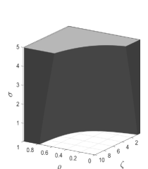
SW Investment JPT Investment (a) (b) S sets       (c) (d) qLL-S sets      

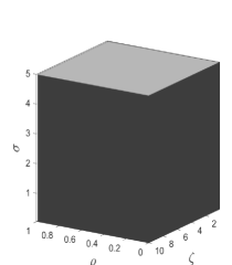
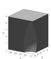
Figure 18: 90% S and qLL-S confidence sets for $\theta=(\rho,\sigma,\zeta)$ derived from the investment Euler equation model (34). Instruments: constant, $\Delta i_{t-2}$, $r_{t-3}^{p}$, $u_{t-2}$. The investment proxies are Fixed Private Investment (left column) and the sum of Gross Private Domestic Investment and Personal Consumption Expenditure on Durable Goods (right column). Newey and West (1987) HAC. Period: 1967Q1-2019Q4.

Appendix F Derivation of Equation (14)

Suppose $x_{t}$ follows (13). Then, its first autocorrelation is $\gamma.$ The pseudo true value of the coefficient $\theta$ in the MA(1) specification (11) is obtained by solving the equation (see Hamilton, 1995, p. 49)

$$\gamma=\frac{\theta^{\ast}}{1+\theta^{\ast 2}},$$ (35)

and we can choose the (unique) invertible solution that satisfies $\left|\theta_{i}\right|<1$. Given $\theta^{\ast},$ the corresponding estimate of the shock in (11), $\omega_{t}^{\ast}$, can be solved from $\left\{x_{t}\right\}$ using the backward recursion

$$\omega_{t}^{\ast}=\sum_{j=0}^{\infty}\left(-\theta^{\ast}\right)^{j}x_{t-j},$$ (36)

while the true structural shock in (13) is simply

$$\omega_{t}=x_{t}-\gamma x_{t-1}.$$

So, we have

$$cov\left(z_{t}^{\ast},\left(z_{t}-z_{t}^{\ast}\right)\right) =cov\left(z_{t}^{\ast},z_{t}\right)+\theta^{\ast 2}var\left(\omega_{t}^{\ast}\right)$$

$$=\frac{\sigma_{\omega}^{2}\gamma\theta^{\ast}}{1-\gamma^{2}}\frac{1}{1-\left(\gamma\theta^{\ast}\right)^{2}}+\theta^{\ast 2}\frac{\left(1-\gamma\theta^{\ast}\right)\sigma_{\omega}^{2}}{\left(1+\gamma\theta^{\ast}\right)\left(1-\gamma^{2}\right)\left(1-\theta^{\ast 2}\right)}$$

$$=\sigma_{\omega}^{2}\theta^{\ast}\frac{\gamma\left(1-\theta^{\ast 2}\right)+\theta^{\ast}\left(1-\gamma\theta^{\ast}\right)^{2}}{\left(1-\left(\gamma\theta^{\ast}\right)^{2}\right)\left(1-\gamma^{2}\right)\left(1-\theta^{\ast 2}\right)},$$ (37)

because

$$cov\left(z_{t}^{\ast},z_{t}\right) =cov\left(\theta^{\ast}\sum_{j=0}^{\infty}\left(-\theta^{\ast}\right)^{j}x_{t-j},\gamma x_{t}\right)$$

$$=\frac{\sigma_{\omega}^{2}\theta^{\ast}\gamma}{1-\gamma^{2}}\sum_{j=0}^{\infty}\left(-\theta^{\ast}\gamma\right)^{j}=\frac{\sigma_{\omega}^{2}\gamma\theta^{\ast}}{1-\gamma^{2}}\frac{1}{1-\left(\gamma\theta^{\ast}\right)^{2}}$$

and

$$x_{t}=\omega_{t}^{\ast}\left(1+\theta^{\ast}L\right)=\omega_{t}\left(1-\gamma L\right)^{-1},$$

so $\omega_{t}^{\ast}$ is an AR(2) process, $\omega_{t}^{\ast}\left(1-a_{1}L-a_{2}L^{2}\right)=\omega_{t},$ with $a_{1}=\gamma-\theta^{\ast},$ and $a_{2}=\gamma\theta^{\ast},$ and therefore, its variance is given by (see Hamilton, 1995, p. 58)

$$var\left(\omega_{t}^{\ast}\right) =\frac{1-a_{2}}{1+a_{2}}\frac{\sigma_{\omega}^{2}}{\left(1-a_{2}\right)^{2}-a_{1}^{2}}$$

$$=\frac{1-\gamma\theta^{\ast}}{1+\gamma\theta^{\ast}}\frac{\sigma_{\omega}^{2}}{\left(1-\gamma\theta^{\ast}\right)^{2}-\left(\gamma-\theta^{\ast}\right)^{2}}$$

$$=\frac{\left(1-\gamma\theta^{\ast}\right)\sigma_{\omega}^{2}}{\left(1+\gamma\theta^{\ast}\right)\left(1-\gamma^{2}\right)\left(1-\theta^{\ast 2}\right)}.$$

Substituting for $\gamma$ using $\theta^{\ast}$ from (35) in (37), we get

$$cov\left(z_{t}^{\ast},\left(z_{t}-z_{t}^{\ast}\right)\right)=\frac{\sigma_{\omega}^{2}\theta^{\ast 2}\left(2-\theta^{\ast 4}\right)\left(\theta^{\ast 2}+1\right)^{2}}{\left(1-\theta^{\ast 2}\right)\left(1-\theta^{\ast}+\theta^{\ast 2}\right)\left(1+\theta^{\ast}+\theta^{\ast 2}\right)\left(1+2\theta^{\ast 2}\right)}\neq 0.$$

References

- Agca and Mozumdar (2017) Agca, S. and A. Mozumdar (2017). Investment-Cash Flow Sensitivity: Fact or Fiction. Journal of Quantitative and Financial Analysis 00(00), 1–31.
- Almeida and Campello (2007) Almeida, H. and M. Campello (2007). Financial constraints, asset tangibility and corporate investment. The Review of Financial Studies 20(5), 1429–1460.
- Altig et al. (2011) Altig, D., L. J. Christiano, M. Eichenbaum, and J. Lindé (2011). Firm-specific capital, nominal rigidities and the business cycle. Review of Economic Dynamics 14(2), 225–247.
- Andrews and Stock (2007) Andrews, D. W. and J. H. Stock (2007). Testing with many weak instruments. Journal of Econometrics 127(1), 24–46.
- Arias et al. (2020) Arias, J. E., G. Ascari, N. Branzoli, and E. Castelnuovo (2020). Positive trend inflation and determinacy in a medium-sized new keynesian model. International Journal of Central Banking 16(3), 51–94.
- Ascari et al. (2021) Ascari, G., L. M. Magnusson, and S. Mavroeidis (2021). Empirical evidence on the Euler equation for consumption in the US. Journal of Monetary Economics 117, 129–152.
- Basu and Bundick (2017) Basu, S. and B. Bundick (2017). Uncertainty shocks in a model of effective demand. Econometrica 85(3), 937–958.
- Bloom (2009) Bloom, N. (2009). The impact of uncertainty shocks. Econometrica 77(3), 623–685.
- Bond and Meghir (1994) Bond, S. and C. Meghir (1994). Dynamic Investent Models and the Firm’s Finacial Policy. The Review of Economic Studies 61(2), 197–222.
- Brault and Khan (2020) Brault, J. and H. Khan (2020). the Shifts in Lead-Lag Properties of the U.S. Business Cycle. Economic Inquiry 58(1), 319–334.
- Christiano et al. (2005) Christiano, L. J., M. Eichenbaum, and C. L. Evans (2005). Nominal rigidities and the dynamic effects of a shock to monetary policy. Journal of Political Economy 113(1), 1–45.
- Christiano et al. (2011) Christiano, L. J., M. Eichenbaum, and S. Rebelo (2011). When is the government spending multiplier large? Journal of Political Economy 119(1), 78–121.
- Christiano et al. (2014) Christiano, L. J., R. Motto, and M. Rostagno (2014). Risk shocks. American Economic Review 104(1), 27–65.
- Christiano et al. (2011) Christiano, L. J., M. Trabandt, and K. Walentin (2011). DSGE models for monetary policy analysis. In B. M. Friedman and M. Woodford (Eds.), Handbook of Monetary Economics, Volume 3A, Chapter 7, pp. 285–367. Elsevier.
- Clarida et al. (2000) Clarida, R., J. Galí, and M. Gertler (2000). Monetary Policy Rules and Macroeconomic Stability: Evidence and Some Theory*. The Quarterly Journal of Economics 115(1), 147–180.
- Del Negro and Schorfheide (2004) Del Negro, M. and F. Schorfheide (2004). Priors from general equilibrium models for vars. International Economic Review 45(2), 643–673.
- Del Negro and Schorfheide (2009) Del Negro, M. and F. Schorfheide (2009). Monetary policy analysis with potentially misspecified models. American Economic Review 99(4), 1415–50.
- Del Negro et al. (2007) Del Negro, M., F. Schorfheide, F. Smets, and R. Wouters (2007). On the fit of new keynesian models. Journal of Business & Economic Statistics 25(2), 123–143.
- Eberly et al. (2012) Eberly, J., S. Rebelo, and N. Vincent (2012). What explains the lagged-investment effect? Journal of Monetary Economics 59, 370–380.
- Fazzari et al. (1988) Fazzari, S., G. Hubbard, B. Petersen, A. Blinder, and J. Poterba (1988). Financing Constraints and Corporate Investment. Brookings Papers on Economic Activity 1, 141–206.
- Foroni et al. (2022) Foroni, C., P. Gelain, and M. Marcellino (2022). The financial accelerator mechanism: does frequency matter? ECB Working Papers Series 2637, European Central Bank.
- Galí and Gertler (1999) Galí, J. and M. Gertler (1999). Inflation dynamics: A structural econometric analysis. Journal of Monetary Economics 44(2), 195–222.
- Groth and Khan (2010) Groth, C. and H. Khan (2010). Investment adjustment costs: An empirical assessment. Journal of Money, Credit and Banking 42(8), 1469–1494.
- Hansen and Singleton (1982) Hansen, L. P. and K. J. Singleton (1982). Generalized instrumental variables estimation of nonlinear rational expectations models. Econometrica 50(5), 1269–1286.
- Hayashi (1982) Hayashi, F. (1982). Tobin’s marginal q and average q: A neoclassical interpretation. Econometrica 50(1), 213–224.
- Inoue et al. (2020) Inoue, A., C.-H. Kuo, and B. Rossi (2020). Identifying the sources of model misspecification. Journal of Monetary Economics 110, 1–18.
- Ireland (2004) Ireland, P. N. (2004). Technology shocks in the new keynesian model. Review of Economics and Statistics 86(4), 923–936.
- Iskrev (2010) Iskrev, N. (2010). Local identification in DSGE models. Journal of Monetary Economics 57(2), 189–202.
- Jurado et al. (2015) Jurado, K., S. C. Ludvigson, and S. Ng (2015). Measuring uncertainty. American Economic Review 105(3), 1177–1216.
- Justiniano et al. (2010) Justiniano, A., G. E. Primiceri, and A. Tambalotti (2010). Investment shocks and business cycles. Journal of Monetary Economics 57(2), 132–145.
- Kaplan and Zingales (1997) Kaplan, S. and L. Zingales (1997). Do investment cash-flow sensitivities provide useful measures of financing constraints? The Quarterly Journal of Economics, 169–215.
- Keane and Rogerson (2012) Keane, M. and R. Rogerson (2012, June). Micro and Macro Labor Supply Elasticities: A Reassessment of Conventional Wisdom. Journal of Economic Literature 50(2), 464–76.
- Lucas (1967) Lucas, Jr., R. E. (1967). Adjustment costs and the theory of supply. Journal of Political Economy 75(4), 321–334.
- Lucas and Prescott (1971) Lucas, Jr., R. E. and E. C. Prescott (1971). Investment under uncertainty. Econometrica 39(5), 659–681.
- Ludvigson et al. (2020) Ludvigson, S. C., S. Ma, and S. Ng (2020). Uncertainty and business cycles: exogenous impulse or endogenous response? American Economic Journal: Macroeconomics, forthcoming.
- Magnusson and Mavroeidis (2014) Magnusson, L. M. and S. Mavroeidis (2014). Identification using stability restrictions. Econometrica 82(5), 1799–1851.
- Mertens (2010) Mertens, E. (2010). Structural shocks and the comovements between output and interest rates. Journal of Economic Dynamics and Control 34(6), 1171–1186.
- Mikusheva (2021) Mikusheva, A. (2021, February). Many Weak Instruments in Time Series Econometrics. Mimeo, MIT.
- Newey and West (1987) Newey, W. and K. West (1987). A simple, positive semi-definite, heteroscedasticity and autocorrelation consistent covariance matrix. Econometrica 55(3), 703–708.
- Ramey (2011) Ramey, V. A. (2011). Identifying government spending shocks: It’s all in the timing. Quarterly Journal of Economics 126(1), 1–50.
- Ramey (2016) Ramey, V. A. (2016). Defense news shocks, 1889–2015: Estimates based on news sources. Manuscript, University of California San Diego.
- Ramey and Zubairy (2018) Ramey, V. A. and S. Zubairy (2018). Government spending multipliers in good times and in bad: evidence from us historical data. Journal of Political Economy 126(2), 850–901.
- Romer and Romer (2004) Romer, C. D. and D. H. Romer (2004). A new measure of monetary shocks: Derivation and implications. American Economic Review 94(4), 1055–1084.
- Sargent (1989) Sargent, T. J. (1989). Two models of measurements and the investment accelerator. Journal of Political Economy 97(2), 251–287.
- Sargent (2008) Sargent, T. J. (2008). Rational expectations. In S. N. Durlauf and L. E. Blume (Eds.), The New Palgrave Dictionary of Economics, pp. 193–201. London: Palgrave Macmillan UK.
- Smets and Wouters (2007) Smets, F. and R. Wouters (2007). Shocks and frictions in us business cycles: A bayesian dsge approach. American Economic Review 97(3), 586–606.
- Stock and Wright (2000) Stock, J. H. and J. H. Wright (2000). GMM with weak identification. Econometrica 68(5), 1055–1096.
- Taylor (1999) Taylor, M. P. (1999). Real interest rates and macroeconomic activity. Oxford Review of Economic Policy 15(2), 95–113.
- Yogo (2004) Yogo, M. (2004). Estimating the elasticity of intertemporal substitution when instruments are weak. Review of Economics and Statistics 86(3), 797–810.