Uncertainty-aware Cardinality Estimation
by Neural Network Gaussian Process

Abstract.

Deep Learning (DL) has achieved great success in many real applications. Despite its success, there are some main problems when deploying advanced DL models in database systems, such as hyper-parameters tuning, the risk of overfitting, and lack of prediction uncertainty. In this paper, we study cardinality estimation for SQL queries with a focus on uncertainty, which we believe is important in database systems when dealing with a large number of user queries on various applications. With uncertainty ensured, instead of trusting an estimator learned as it is, a query optimizer can explore other options when the estimator learned has a large variance, and it also becomes possible to update the estimator to improve its prediction in areas with high uncertainty. The approach we explore is different from the direction of deploying sophisticated DL models in database systems to build cardinality estimators. We employ Bayesian deep learning (BDL), which serves as a bridge between Bayesian inference and deep learning. The prediction distribution by BDL provides principled uncertainty calibration for the prediction. In addition, when the network width of a BDL model goes to infinity, the model performs equivalent to Gaussian Process (GP). This special class of BDL, known as Neural Network Gaussian Process (NNGP), inherits the advantages of Bayesian approach while keeping universal approximation of neural network, and can utilize a much larger model space to model distribution-free data as a nonparametric model. We show that our uncertainty-aware NNGP estimator achieves high accuracy, can be built very fast, and is robust to query workload shift, in our extensive performance studies by comparing with the existing approaches.

1. Introduction

Table 1. ML/DL Approaches for AQP and Cardinality Estimation

Approach	Supported Queries				Learning Strategy	Model	Model Update
	Join	Selection	Aggregate	Group By
DBEst (DBLP:conf/sigmod/MaT19, )	precomp. join	num., cate.	$\mathsf{cnt}$,$\mathsf{sum}$,$\mathsf{avg}$,etc.	✓	supervised & unsupervised	KDE & GBDT	✗
DeepDB (DBLP:journals/pvldb/HilprechtSKMKB20, )	precomp. join	num., cate.	$\mathsf{cnt}$,$\mathsf{sum}$,$\mathsf{avg}$	✓	unsupervised	SPN	✓
Thirumuruganathan et. al. (DBLP:conf/icde/Thirumuruganathan20, )	✗	num., cate.	$\mathsf{cnt}$,$\mathsf{sum}$,$\mathsf{avg}$	✓	unsupervised	VAE	✗
Kiefer et al. (DBLP:journals/pvldb/KieferHBM17, )	Equi-join	num., cate.	$\mathsf{cnt}$	✗	unsupervised	KDE	✓
Kipf et al. (DBLP:conf/cidr/KipfKRLBK19, )	PK/FK join	num., cate.	$\mathsf{cnt}$	✗	supervised	MSCN	✗
Dutt et al. (DBLP:journals/pvldb/DuttWNKNC19, )	✗	num., cate.	$\mathsf{cnt}$	✗	supervised	NN, GBDT	✗
Dutt et al. (dutt2020efficiently, )	PK/FK join	num., cate.	$\mathsf{cnt}$	✗	supervised	GBDT	✓
Sun et al. (DBLP:journals/pvldb/SunL19, )	PK/FK join	num., cate., str.	$\mathsf{cnt}$	✗	supervised	Tree LSTM	✓
Hasan et al. (DBLP:conf/sigmod/HasanTAK020, )	✗	num., cate.	$\mathsf{cnt}$	✗	unsupervised	MADE	✗
Naru (DBLP:journals/pvldb/YangLKWDCAHKS19, )	precomp. join	num., cate.	$\mathsf{cnt}$	✗	unsupervised	MADE, Transformer	✓
NeuroCard (DBLP:journals/corr/abs-2006-08109, )	Full outer join	num., cate.,	$\mathsf{cnt}$	✗	unsupervised	MADE, Transformer	✓

The learning approaches are shifting from the traditional ML (Machine Learning) models (e.g., KDE, GBDT) to DL (Deep Learning) models (e.g., NN, MSCN, VAE, MADE, Transformer, SPN, LSTM). The shifting is motivated by the powerful approximation capability of neural networks in end-to-end applications and the high efficiency of DL frameworks. Compared with traditional ML, DL has achieved a great improvement on estimation accuracy, and more and more advanced DL architectures are devised to improve the performance of the learning tasks with deeper layers to pursue more powerful modeling capability. In database systems, the DL models have been extensively studied for query optimization (DBLP:journals/pvldb/MarcusNMZAKPT19, ), index recommendation (DBLP:conf/sigmod/DingDM0CN19, ), view materialization (DBLP:journals/corr/abs-1903-01363, ), and cardinality estimation (DBLP:journals/pvldb/KieferHBM17, ; DBLP:conf/cidr/KipfKRLBK19, ; DBLP:journals/pvldb/DuttWNKNC19, ; dutt2020efficiently, ; DBLP:journals/pvldb/SunL19, ; DBLP:conf/sigmod/HasanTAK020, ; DBLP:journals/pvldb/YangLKWDCAHKS19, ; DBLP:journals/corr/abs-2006-08109, ). Despite the success of DL approaches, the complex DL approaches incur some main problems in general.

The first is hyper-parameters, on which the performance of DL models highly relies, including the training hyper-parameters and network architecture configurations. Note that onerous effort of parameter tuning must be paid to pursuing satisfying performance, which is labor-intensive. Although autoML tools (hutter2019automated, ) have been developed to avoid human-in-the-loop, deploying such tools in database systems needs great effort as searching a suitable hyper-parameter combination needs a huge number of trials with high computation cost. It is worth mentioning that a well-tuned model for one database is difficult to transfer to other databases, which means that the retraining/tuning needs repeating when the underlying data changes significantly.

The second is a high risk of overfitting that DL models are exposed to. Subject to a particular family of function designed, general DL models are indexed by a large number of parameters, fully fitted by the training data. It is assumed testing data is from the same underlying distribution of the training data, otherwise the prediction may have a large variance. Many regularization techniques can be used, but they can only alleviate the problem to some degree. Collecting more data to enhance training helps to reduce the variance. But this means a higher cost for acquiring the data/ground truth and training.

The third is prediction belief, which is an important issue we focus on in this work. The issue is that DL models cannot capture and convey their prediction belief, namely, how probably their prediction is accurate or how much is the prediction uncertainty. The uncertainty comes from different sources, for example, the noise of the training data, the dissimilarity of the test data from the training data, the mismatching of the model class to the data to be described. For classification tasks, DL models predict the probability distribution that one data point is associated with the candidate classes by a $\mathsf{softmax}$ function, which is shown to be over-confident on the most likely class (DBLP:conf/icml/GuoPSW17, ). For regression tasks (e.g., cardinality estimation), DL models can only output a scalar value without any uncertainty measurements of the prediction, such as variance and confidential interval. It is highly desirable to avoid situations where we have no choices but trust the DL predictions being made in database systems. In other words, as a database system to support a large number of users in various applications, where user queries may be different and databases will be updated from time to time, what database systems require is not only an accurate model prediction, but also an indication of how much the predictions can be trusted regarding the learned model.

In this paper, we study cardinality estimation for SQL queries with selection, projection and join. We focus on uncertainty. The approach we take can also address the hyper-parameter and risk of overfitting. Table 1 summarizes the recent ML/DL approaches studied for AQP (Approximate Query Processing) (the top three) and cardinality estimation (the bottom eight). These approaches are categorized into supervised learning approaches and unsupervised learning approaches. The supervised learning approaches are query-driven, which learn a function that maps the query features to its cardinality. The unsupervised learning approaches are data-driven, which learn the joint probability distribution of the underlying relational data. The supervised learning approaches are easy to deploy with relatively low training and prediction overhead, however, they lack robustness to shifting query workloads. On the contrary, the unsupervised learning approaches are robust to different query workloads. But, building a model consumes many resources as large volumes of data need to be fed into the model multiple times. For example, for a single relation within 100MB, the unsupervised learning estimators DeepDB (DBLP:journals/pvldb/HilprechtSKMKB20, ) and NeuroCard (DBLP:journals/corr/abs-2006-08109, ) take hundreds and thousands of seconds to train a model on a 56-core CPU, which is 2-3 orders slower than the lightweight supervised learning estimators (DBLP:journals/pvldb/DuttWNKNC19, ). Furthermore, the unsupervised estimators suffer from underestimation for range queries as the prediction is conducted by integration over the learned distribution regarding the query condition. In this work, we study cardinality estimation based on a supervised approach with an uncertainty guarantee. Consider cardinality estimation for an SQL query. If a DL-based estimator provides an estimate without uncertainty, the optimizer used can only take it as it is. If a DL-based estimator provides an additional probability distribution with mean, say $\mu$, and standard deviation, say $2\mu$, as its predictive cardinality. Then, the query optimizer can take it as inaccurate since the coefficient of variation is up to 2, and the optimizer can either explore other options or use the built-in estimator for query planning. It is important that the system is aware that the estimator may be outdated and need retraining, if the learned estimator delivers a low confidence level for a large fraction of arrival queries. Till now, all the DL-based cardinality approaches cannot provide the prediction uncertainty.

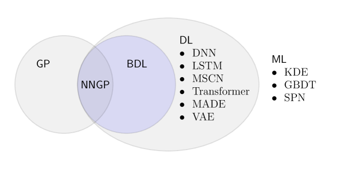
Figure 1. From ML/DL estimators To NNGP (GP & BDL)

In this work, different from the direction of deploying sophisticated DL models in database systems, we employ Bayesian deep learning (BDL) to build cardinality estimators, where BDL serves as a bridge between Bayesian inference and deep learning (DBLP:journals/tkde/WangY16, ). In a nutshell, BDL imposes a prior distribution on the neural network weights, and the derived models are ensembles of neural networks in a particular function space, which output a distribution as the prediction. The prediction distribution provides principled uncertainty calibration for the prediction. This uncertainty helps the model to improve itself explicitly, by collecting the information of testing data with higher uncertainty and retraining/fine-tuning the model. In addition, the prediction distribution by BDL is robust to the overfitting problem. The parameters and hyper-parameters of BDL models are much fewer (i.e., the statistics of the prior distribution and the prior type, respectively), in versus to the parameters and hyper-parameters that need in DL models (i.e., the weights of the neural networks and the network architecture configurations, number of layers, number of hidden units in each layer), and in DL training configurations (i.e., optimization algorithm, learning rate, batch size, epochs, etc.). When the network width of the BDL model goes to infinity, the model performs equivalent to Gaussian Process (GP) (neal1996priors, ), named Neural Network Gaussian Process (NNGP). Exact Bayesian inference can be used to train this special GP as a lightweight cardinality estimator, while offering a more powerful generalization capability than a finite wide neural network. NNGP keeps the flexible modeling capability of deep learning, while offering robustness and interpretability by Bayesian inference. Fig. 1 delineates the extraordinary standpoint of our NNGP estimator among the existing ML/DL-based estimators in Table 1, for cardinality estimation. Here, KDE and GBDT are classical ML models while SPN is a new type of probabilistic graphical model with deeper layers. DL models are associated with different neural network architectures. A BDL model is a special kind of DL model in which the neural network parameters are probability distributions. We explore a new model, named NNGP, which is the BDL model with infinite wide hidden layers, and can be built using GP.

Contribution. The main contributions of this paper are summarized as follows. ➊ We employ an advanced BDL model, named Neural Network Gaussian Process (NNGP), to build cardinality estimators for relational database systems. Our NNGP estimator can support range queries on single relations and equi/theta-join on multiple relations for a database. To the best of our knowledge, this is the first exploration of BDL approaches for database applications. ➋ As the first DL-based cardinality estimator which supports principled uncertainty estimation, we investigate the uncertainty that NNGP captures, compared with existing uncertainty quantification approaches for DL. ➌ We conduct extensive experimental studies to verify the effectiveness and efficiency of NNGP estimator via comparison with recent ML/DL based estimators. The NNGP estimator distinguishes from existing estimators by its swift model construction and prediction, robustness to workload shifts, and appealing accuracy.

Roadmap. section 2 gives the problem statement. In section 3, we give an overview of the NNGP estimator, and introduce Bayesian learning, GP and NNGP in section 4. Then, we elaborate on the uncertainty calibration of NNGP in section 5.  section 6 reports the experimental results. Finally, we review the related works in section 7 and conclude the paper in section 8.

2. Problem Statement

A relational database consists of a set of relations, $\{R_{1},R_{2},\cdots,R_{N}\}$, where a relation $R_{i}$ has $d_{i}$ attributes such as $R_{i}=(A_{1},\cdots A_{d_{i}})$. Here, an attribute $A_{j}$ is either a numerical attribute in a domain with given range $[min_{j},max_{j}]$ or a categorical attribute with a discrete finite domain $\{c_{1},c_{2},\cdots c_{m_{j}}\}$.

We study cardinality estimation for the select-project-join SQL queries with conjunctive conditions. A selection on an attribute is either a range filter (i.e., $[lb_{j},ub_{j}]$, denoting the condition $lb_{j}\leq A_{j}\leq ub_{j}$), if the attribute is numerical, or $\mathsf{IN}$ filter (i.e., $A_{j}~{}{\mathsf{IN}}~{}C$, $C\subset\{c_{1},c_{2},\cdots c_{m_{j}}\}$, denoting the condition $\exists c_{k}\in C,A_{j}=c_{k}$), if the attribute is categorical. A projection can be on any attributes. A join can be equi/theta-join. For joining over numerical attributes, the join condition can be $\{<,\leq,=,>,\geq,\neq\}$. For joining over categorical attributes, the join condition is either $=$ or $\neq$, as the categorical domain is order-free. The primary-foreign key join, or PK/FK-join, is treated as a special equi-join with the extra constraints. We also support self-joins, which are conducted by renaming the same relations. An example is given below.

$$\sigma_{(100\leq R_{1}.A_{1}\leq 200)\land(R2.A_{2}~{}{\mathsf{IN}}~{}\{15,20,25\})}\displaystyle{(R_{1}\mathop{\Join}_{\begin{subarray}{c}R_{1}.A_{3}\leq R_{2}.A_{3}\end{subarray}}R_{2})}$$

where $\sigma$ is the select operator and $\Join$ is a join operator. It is worth mentioning that we support general select-project-join SQL queries. All the existing learned estimators do not support joins other than PK/FK joins. For example, (DBLP:journals/corr/abs-2006-08109, ) does not support cyclic join queries and selection conditions on join attributes and (DBLP:journals/pvldb/HilprechtSKMKB20, ) does not support multiple selection conditions on join attributes.

The cardinality of an SQL query $q$ is the number of resulting tuples, denoted as $c(q)$. To learn a cardinality estimation, like the existing work, we require a set of joinable attribute pairs $\{(R_{1}.A_{i},R_{2}.A_{j}),$ $\cdots\}$, in addition to a set of relations $\{R_{1},\cdots R_{N}\}$. For example, two relations $\{R_{1},R_{2}\}$ with joinable attribute pairs $\{(R_{1}.A_{3},R_{2}.A_{3})\}$.

The Problem Statement: Given a set of relations and a set of joinable attribute pairs, learn a model $\mathcal{M}:q\mapsto\mathbb{R}$ from a training query set $\{(q_{1},c(q_{1})),$ $(q_{2},c(q_{2})),\cdots\}$, where $q_{i}$ is an SQL select-project-join query and $c(q_{i})$ is its actual cardinality, to predict the cardinality for unseen queries.

We use $\mathsf{q}$-$\mathsf{error}$ to evaluate the accuracy of the estimated value.

(1) $${\mathsf{q}}\mbox{-}{\mathsf{error}}(q)=max\bigg{\{}\frac{c(q)}{\hat{c}(q)},\frac{\hat{c}(q)}{{c}(q)}\bigg{\}}$$

Intuitively, $\mathsf{q}$-$\mathsf{error}$ quantifies the factor by which the estimated count ($\hat{c}(q_{i})$) differs from the true count ($c(q_{i})$). It is symmetrical and relative so that it provides the statistical stability for true counts of various magnitudes. Here, we assume $c(q)\geq 1$ and $\hat{c}(q)\geq 1$.

We learn an uncertainty-aware model, and we do not make any assumptions on data and query, e.g., the distribution of attribute values, the independence of attributes and relations, the distribution of the selection/join conditions of the queries, etc.

Query Encoding: Following the existing work, a select-project-join query we support can be encoded by a fixed length vector. The encoding consists of two parts: the selection conditions and the join conditions. The two parts are encoded separately and concatenated as follows.

For selection condition, the encoding of all the attributes in all the relations of the schema are concatenated by a fixed order (e.g., lexicographical order). In a similar manner, for the join conditions, the encoding of all the join pairs are concatenated.

The selection conditions are specified on numerical/categorical attributes. For a range filter, $lb_{j}\leq A_{j}\leq ub_{j}$, on a numerical attribute $A_{j}$, we normalize $lb_{j}$ and $ub_{j}$ to $[0,1]$ by mapping $[lb_{j},ub_{j}]$ to $[\frac{lb_{j}-min_{j}}{max_{j}-min_{j}},\frac{ub_{j}-min_{j}}{max_{j}-min_{j}}]$, where $[min_{j},max_{j}]$ is the domain of the attribute $A_{j}$. Thus, the representation is the interval of two real values. For an $\mathsf{IN}$ filter, $A_{j}~{}{\mathsf{IN}}~{}C$, on a categorical attribute $A_{j}$, where $C$ is a subset of the attribute $A_{j}$’s domain $\{c_{1},c_{2},\dots c_{m}\}$, a straightforward encoding is to build an $m$-dim bitmap where its $k$-th bit is 1 if $c_{k}\in C$, otherwise 0. This binary representation is effective for attributes with small domain, however, it is difficult to scale on a large domain where the predicate vector is high-dimensional and sparse. Therefore, for a large domain, we adopt the factorized bitmap (DBLP:journals/corr/abs-2006-08109, ), i.e., slicing the whole bitmap to chunks, and converting each chunk into corresponding base-10 integer. Finally, the selection condition is represented losslessly by $\lceil m/s\rceil$ integers, where $s$ is the length of the chunk.

Regarding join conditions, for each joinable attribute pair $(A_{i},A_{j})$, we use a 3-bit bit-map to encode the join condition on this pair, corresponding to the 3 comparison operators, $<,=,>$, respectively, where ‘1’ denotes there is a comparative condition on $(A_{i},A_{j})$. For example, $A_{i}<A_{j}$, $A_{i}\geq A_{j}$, and $A_{i}\neq A_{j}$ are encoded as ‘100’, ‘011’ and ‘101’, respectively. The bit-map ‘000’ denotes that the query is free of join condition on the pair.

3. An Overview

We present an NNGP overview for cardinality estimator that learns a DL model using GP. We discuss NNGP from the viewpoints of standard neural network and GP, where NNGP exhibits the approximation capability of neural network and can be solved by exact Bayesian inference as a regular GP. Such NNGP properties enable our cardinality estimator to be robust, lightweight, and uncertainty-aware, compared with the existing DL-based estimators. We show the differences between a neural network and NNGP in Fig. 2.

On the left, Fig. 2 shows a standard fully-connected neural network, which is the building block of all the DL-based estimators in Table 1. The hidden layer is a weighted linear transformation with nonlinearity that transforms input representation to output in a layer by layer fashion. Given an empirical loss function, the parameters (i.e., the weights of the linear transformation) fit to given training data (i.e., the vectorized relational data or SQL query regarding cardinality estimation) by forward-backward propagation algorithm. As a parametric model, the prediction on new input is determined by the learned parameters. Theoretically, neural network is able to approximate any given continuous function (DBLP:journals/nn/HornikSW90, ; DBLP:journals/nn/Hornik91, ), and achieve an arbitrary small approximation error with infinite wide hidden layers.

On the right, Fig 2 shows NNGP, which is a special class of Bayesian DL model, whose hidden layer has an infinite number of neurons. In statistical learning, Bayesian inference is a principled way to describe prediction belief. Bayesian DL is derived from developing Bayesian inference on modern DL (DBLP:journals/tkde/WangY16, ). Specifically, prior distributions are imposed on the parameters of the neural network. In other words, given a set of training data, the posterior distribution of parameters is inferred by Bayes rule. And the prediction of a new input is a probabilistic distribution computed by Bayesian model average that ensembles all the models in the parameters space weighted by the posterior of the parameters. NNGP, as a special type of Bayesian DL, is equivalent to GP in the sense that any finite collection of outputs is a Gaussian distribution, and its output is a summation of an infinite number of i.i.d. random variables implied by Central Limit Theorem (neal1996priors, ). The infinite hidden neurons are composed of the set of GP basis functions, leading to a parametric, non-stationary GP kernel. Compared with regular GP with stationary kernels, this DL-based kernel is more flexible to adapt to the underlying data by exploiting the representation learning ability of DL. Our testing in section 6 shows that without DL, a simple GP estimator fails to achieve an approaching or better performance, compared with the DL cardinality estimators.

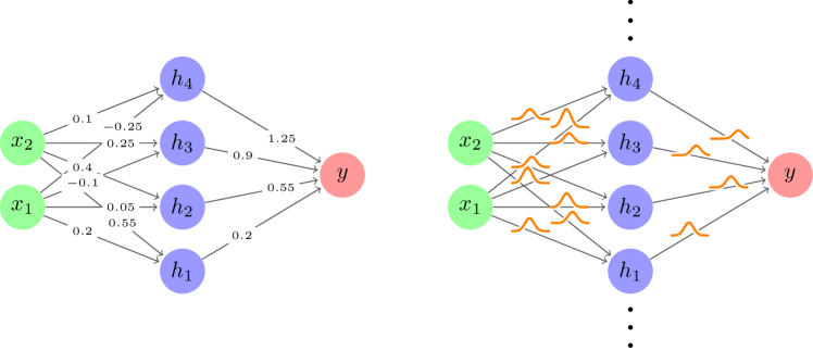
Figure 2. Neural Network (left) vs. NNGP (right)

From the perspective of Bayesian DL, NNGP inherits the advantages of Bayesian approach while keeping the universal approximation of neural network. With the parameter prior, NNGP converts from neural network parameter learning to the prior’s hyper-parameter learning so that it overcomes the over-parametrization of neural network. Instead of betting on one parameter configuration, NNGP ensembles an infinite number of plausible neural network models in the space of a given architecture and prior family, thereby provides a robust approximation. The predictive distribution naturally conveys the prediction uncertainty regarding the model’s posterior and indicates out-of-distribution testing points.

From the perspective of GP, NNGP is a nonparametric model with the infinite number of basis functions. Here, nonparametrics does not mean the model is parameter-free, but in the sense that the model can not be specified in a finite number of parameters. As a nonparametric model, NNGP utilizes a much larger model space to model distribution-free data. In other words, it does not assume data to be modeled is i.i.d. or generated from a specified distribution as what DL models require (lee2004bayesian, ). The property of distribution-free promotes deploying database-oriented learning tasks (e.g., cardinality estimation), since real data and queries in DBMS are too large and diverse. It is difficult to assume that they are subject to some distribution where both data and queries may evolve over time. Therefore, compared to general DL models, NNGP does not require large volume training samples to approximate an i.i.d. assumption. In addition, the learning paradigm of NNGP converts from parameter learning for DL to kernel learning for GP, which avoids the approximation inference of Bayesian DL by manipulating the infinite wide neural network implicitly. More concretely, NNGP under certain neural network configuration (e.g., $\mathsf{ReLU}$ nonlinearity) has an analytical kernel function, which means training and prediction of this special type of DL model can be solved by pure statistical method in closed-form (i.e., exact Bayesian inference) as for a regular GP. In our experiments of section 6, we verify training an NNGP estimator on the fly only consumes several seconds, up to 1-2 orders faster than corresponding DL estimators.

We show NNGP, as a kernel method, from the point of neural network enhanced kernel function in Fig. 3. In Fig. 3, we visualize two kernel matrices of NNGP estimator by taking vectorized SQL queries as the input, which are created by $500$ training queries and $500$ test queries. The queries for Fig. 3(a) are on a single relation $\mathsf{forest}$, with $2\sim 10$ selection conditions, while the queries for Fig. 3(b) are join queries over $0\sim 5$ relations in $\mathsf{TPC}$-$\mathsf{DS}$. The kernel matrices are ordered by the number of selection/join conditions for the training query and the coefficient of variation of the predictive distribution for the test query. In Fig. 3, the lighter the color, the larger the inner product of the infinite hidden representations of a train-test query pair, which indicates the larger the similarity between the pair. There are two key observations. First, the uncertainty of the prediction of a test query is highly correlated with its similarity to the training queries. The lower the uncertainty, the larger the similarity to all the 500 training queries. This observation supports our intuition. Second, a query with more join conditions tends to be more dissimilar to other queries. The NNGP kernel provides a simple yet effective mechanism to compare input similarity regarding transformed infinite feature space. The knowledge of the training data is persisted in the kernel matrix to smooth the prediction, with similarity measures between training/testing data.

We discuss NNGP with the existing DL approaches for cardinality estimation following a recent experimental study in (DBLP:journals/corr/abs-2012-06743, ) that analyzes and compares 5 learned cardinality estimators over single relation. In (DBLP:journals/corr/abs-2012-06743, ), the authors identify a set of behavior logics, as the inductive biases the learned estimators are expected to capture, namely, consistency, monotonicity, stability, and fidelity. All the query-driven DL estimators only preserve the stability as they model the estimation as a regression task. The data-driven DL estimator NeuroCard supports fidelity but cannot satisfy others, whereas the data-driven DL estimator DeepDB satisfies all the logics since it relies on hierarchical density factorization. Our NNGP estimator is a supervised learning based estimator. Thereby NNGP only supports stability like all the other query-driven regressors. However, the NNGP estimator distinguishes from the existing learned estimators from its small tuning cost and swift model construction, which are promising for fast adaption in dynamic environments. NNGP supports Bayesian based uncertainty quantification regarding the acquired knowledge, and kernel learning enables kernel based feature understanding and selection (DBLP:journals/jmlr/SongSGBB12, ; DBLP:conf/nips/ChenSWJ17, ).

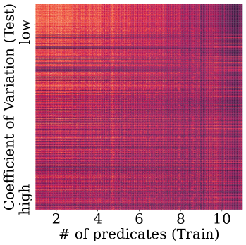
(a) $\mathsf{forest}$

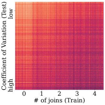
(b) $\mathsf{TPC}$-$\mathsf{DS}$

Figure 3. Test-Train Kernels of NNGP

Finally, the way we use GP is different from GP used for database configuration tuning (DBLP:conf/sigmod/AkenPGZ17, ; DBLP:journals/pvldb/DuanTB09, ). First, in (DBLP:conf/sigmod/AkenPGZ17, ; DBLP:journals/pvldb/DuanTB09, ), GP is used to model the concerned performance given a set of input configurations, and Bayesian optimization is used to search for a better one among a set of configurations. In our approach, the GP regressor is the cardinality estimator. Second, the GP used in (DBLP:conf/sigmod/AkenPGZ17, ; DBLP:journals/pvldb/DuanTB09, ) is equipped with stationary kernel functions. For cardinality estimation with a larger feature space (i.e., the query space and a higher requirement of accurate prediction), stationary kernel functions are not flexible in terms of adapting to the input data. We use non-stationary kernel functions that belong to a particular type of neural network.

4. NNGP: from NN to GP

In this section, we discuss Bayesian learning, and its difference from standard learning, introduce GP and present NNGP.

4.1. Bayesian Learning

In standard parametric ML/DL, a model to learn is a function of input $x$, $f(x,w)$, parameterized by $w$. Learning is to optimize a specified loss function $\mathcal{L}(f(x,w),y)$ to fit the parameter $w$ to training data $(x,y)$ in a training set $(X,Y)$. In contrast to learning by optimization, Bayesian learning is to learn by marginalization. The parameter $w$ is assumed to be a random variable drawn from a prior distribution $p(w)$. Given the observed training data $(X,Y)$, the posterior distribution of $w$ can be inferred by Bayes rule (Eq. (2)).

(2) $$p(w|Y,X)=\frac{p(Y|X,w)p(w)}{p(Y|X)}=\frac{p(Y|X,w)p(w)}{\int p(Y|X,w)p(w)dw}$$

To infer the target value for testing data $X^{*}$, the predictive probability $p(Y^{*}|X^{*},Y,X)$ is computed by applying the probabilistic sum and product rules, assuming the training and testing are conditional independent regarding $w$.

(3) $$p(Y^{*}|X^{*},Y,X)=\int p(Y^{*}|X^{*},w)p(w|Y,X)dw$$

The predictive distribution of Eq. (3) represents Bayesian model average (DBLP:conf/nips/WilsonI20, ). That is, instead of relying on a single prediction of one model with a single configuration of parameters, Eq. (3) ensembles all the models with all possible configurations of the parameters ${w}$, weighted by the posterior of the parameters, $p({w}|{Y},{X})$, from Eq. (2), by marginalization of $w$. Therefore, the predictive distribution does not depend on any specific parameter configuration. In contrast, classical training of parametric model aims to find one configuration $\hat{{w}}$ that maximizes the likelihood of the observed data or minimizes the empirical loss in equivalence. In other words, the posterior distribution $p({w}|{Y},{X})=1$ for ${w}=\hat{{w}}$ and $0$ otherwise, leading to the model inference as Eq. (4).

(4) $$p(Y^{*}|{X}^{*},Y,{X})=p(Y^{*}|{X}^{*},\hat{{w}}),\hat{{w}}=\mathop{\arg\max}\limits_{{w}}p(Y|{X},{w})$$

Comparing the inference of Eq. (3) and Eq. (4), if the weights posterior $p({w}|{Y},{X})$ has a flat distribution and $p({Y}^{*}|{X}^{*},\hat{{w}})$ varies significantly where the posterior has mass, the discrepancy of prediction by Bayesian model average and classical approach tends to be large. One well-known reason is the observed data is insufficient or deviating from the features of the test data, where the observed data cannot well infer the weight posterior in principle. The Bayesian learning calibrates this kind of uncertainty, a.k.a., epistemic uncertainty.

$f(x)=\bm{w}x+b$

$f(x)=\bm{w}x+b$ $\bm{w}\sim\mathcal{N}(0,\sigma^{2}_{w})$, $b\sim\mathcal{N}(0,\sigma^{2}_{b})$

(a) Linear Regression

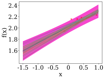
(b) Bayesian Linear Regression

Figure 4. LR vs. BLR

Example 4.1.

A simple example of Linear Regression (LR) and Bayesian Linear Regression (BLR) is shown in Fig. 4 to illustrate the differences between standard learning and Bayesian learning. In LR (Fig. 4(a)), a linear function $f(x)=wx+b$ is used to fit the training data points, minimizing the square error. The parameters $w$ and $b$ can be solved analytically by least squares or gradient descent. In BLR (Fig. 4(b)), it does not aim to solve a deterministic value for $w,b$, instead the posterior distributions of $w$, $b$ are computed, given the training data, assuming the priors of $w,b$ are simple Gaussian distributions with zero means. The model is no longer a linear function but a random variable determined by its parameter posterior, which forms a function space with infinite linear functions. The color lines in Fig. 4(b) indicate some samples in the function space. The derived predictive distribution (Eq. (3)) of BLR is a Gaussian distribution, thereby the shaded area in Fig. 4(b) delineates the 95%-confidential interval. We can observe that in the range with few training data, i.e., $x\in[-1.5,-0.5]$, the predictive uncertainty tends to be large, reflect to the fanout of the sampled functions and wider confidential interval. BLR only has two hyper-parameters to be set, which are the variances $\sigma^{2}_{w}$, $\sigma^{2}_{b}$ of the parameter prior. The hyper-parameters can be tuned by Bayesian model selection (DBLP:books/lib/RasmussenW06, ).

4.2. Gaussian Process

Given a set of $N$ training data points ${X}=\{{x}_{1},\cdots,{x}_{N}\}$ and a model $f({x})$, GP is used in modeling the joint distribution of the model’s predictions $f({X})=\{f({x}_{1}),\cdots,f({x}_{N})\}$. Consider a simple linear model in Eq. (5), with fixed basis function $\phi(\cdot)=\{\phi_{1},\cdots,\phi_{m}\}$, (e.g., polynomial, radial basis function), which is a projection from original input to a feature space.

(5) $$f({X})=\sum_{j=1}^{m}w_{j}\phi_{j}({X})=\bm{\Phi}{w}$$

In Eq. (5), $\bm{\Phi}\in\mathbb{R}^{N\times m}$ is the design matrix where $\bm{\Phi}_{nj}=\phi_{j}({x}_{n})$, i.e., the value of the $j$-th basis function for the $n$-th data point. Suppose a zero mean Gaussian prior is put on the weights ${w}$, where $\mathcal{I}\in\mathbb{R}^{N\times N}$ is the Identity matrix.

(6) $${w}\sim\mathcal{N}(\bm{0},\sigma_{w}^{2}\mathcal{I})$$

Since $f({X})$ is a linear transformation of ${w}$, $f({X})$ is also a Gaussian distribution as Eq. (7), where ${\epsilon}\sim\mathcal{N}(\bm{0},\sigma_{\epsilon}^{2}\mathcal{I})$ is an extra noise on $f({X})$.

(7) $$f({X})\sim\mathcal{N}(\bm{0},\sigma_{w}^{2}\bm{\Phi}\bm{\Phi}^{T}+\sigma_{\epsilon}^{2}\mathcal{I})$$

Here, Eq. (7) shows the function $f({x})$, as a random variable, is a Gaussian process by definition such that for any finite selection of points ${X}$, $f({X})$ is a joint Gaussian distribution (mackay1998introduction, ). The covariance matrix $\mathsf{K}_{X,X}=\sigma_{w}^{2}\bm{\Phi}\bm{\Phi}^{T}+\sigma_{\epsilon}^{2}\mathcal{I}$, a.k.a., the kernel matrix, models the similarity of data points. Specifically, the entry $\mathsf{K}_{ik}=\sigma_{w}^{2}\langle\phi({x}_{i}),\phi({x}_{k})\rangle+\sigma_{\epsilon}^{2}\mathcal{I}_{ik}$ measures the similarly of points ${x}_{i},{x}_{k}$ under basis function $\phi(\cdot)$. A simplest example is that $\phi(\cdot)$ is the identity function, i.e., $\phi({x})={x}$, its model is equivalent to BLR.

To make prediction for testing data points ${X}^{*}=\{x^{*}_{1},\cdots,x^{*}_{M}\}$, we need to compute the conditional distribution $p(f({X}^{*})|f({X}))$ as the prediction. It is also proved to be a Gaussian distribution as Eq. (8), where $\mathsf{K}_{X,X}\in\mathbb{R}^{N\times N}$, $\mathsf{K}_{X,X^{*}}\in\mathbb{R}^{N\times M}$, $\mathsf{K}_{X^{*},X^{*}}\in\mathbb{R}^{M\times M}$ are the ${X},{X}$ kernel, ${X},{X}^{*}$ kernel and ${X}^{*},{X}^{*}$ kernel matrices, respectively.

(8) $$f({X}^{*}) |f({X})\sim\mathcal{N}({\mu},{C})$$

(9) $${\mu} =\mathsf{K}_{X,X^{*}}^{T}\mathsf{K}_{X,X}^{-1}f({X})$$

(10) $${C} =\mathsf{K}_{X^{*},X^{*}}-\mathsf{K}_{X,X^{*}}^{T}\mathsf{K}_{X,X}^{-1}\mathsf{K}_{X,X^{*}}$$

Given the ground truth of the training data ${X}$, denoted as $Y$, and the prediction target for ${X}^{*}$ is ${Y}^{*}$, the expectation of the prediction is $\mathbb{E}[Y^{*}]=\mathsf{K}_{X,X^{*}}^{T}\mathsf{K}_{X,X}^{-1}{Y}$, derived from Eq. (9). Assume a matrix of functions ${h}({X}^{*})=\mathsf{K}_{X,X^{*}}^{T}\mathsf{K}_{X,X}^{-1}$, we have $\mathbb{E}[f({X}^{*})]={h}({X}^{*})Y$, indicating GP regression is a weighted linear smoother over the observed target value $Y$. The weight function ${h}$ is determined by the train-train and train-test kernels. Meanwhile, the diagonal element of matrix ${C}$ in Eq. (9) measures the variance of the prediction. With this predictive Gaussian distribution, we can easily compute the $\delta$-confidential interval of $f({x}^{*})$ as $[\mu_{x^{*}}-{q}_{\delta}diag(C)_{x^{*}},\mu_{x^{*}}+{q}_{\delta}diag(C)_{x^{*}}]$, where $q_{\delta}$ is the $\delta$-quantile of $\mathcal{N}(0,1)$. Intuitively, the expectation $\mathbb{E}[{y}^{*}]$ should be treated as the explicit prediction $\hat{y}$. In practical applications, as it aims to minimize the predictive loss given an empirical loss function, the prediction is to find $\hat{y}$ that minimize the expected loss by averaging the empirical loss $\mathcal{L}_{{\mathsf{exp}}}$ w.r.t. the predictive distribution as Eq. (11).

(11) $$\mathcal{L}_{{\mathsf{exp}}}=\int\mathcal{L}_{{\mathsf{emp}}}({y}^{*},{\hat{y}})p(y^{*}|x^{*},Y,X)dy^{*}$$

4.3. Neural Network Gaussian Process

GP is a stochastic process with a fixed basis function. If the basis is fixed, the model is linear w.r.t. the parameters, and the kernel function $\mathsf{K}$ as well as the predictive distribution (Eq. (8)) are analytically tractable. The limitation of a fixed basis function is its incapability of adapting to the training data. In general, a model with an adaptive basis function (e.g., neural networks) can be a potential extension, but it is much difficult to treat it analytically (DBLP:books/lib/RasmussenW06, ). To address it, the authors in (neal1996priors, ) show that there is a special case where the neural network has an infinite number of hidden units. With such findings, some complex neural network architectures with infinite wide hidden layers are proved to be GP such as convolutional neural network (DBLP:conf/iclr/NovakXBLYHAPS19, ; DBLP:conf/iclr/Garriga-AlonsoR19, ), recurrent neural network (DBLP:conf/nips/Yang19, ), attention (DBLP:conf/icml/HronBSN20, ) and graph neural network (DBLP:journals/corr/abs-2002-12168, ).

We discuss the foundation, the infinite wide multilayer perceptrons which we use for cardinality estimation. We explain it using a single hidden layer feed forward neural network, $f({x})$, which takes $d$-dim vector ${x}=[x_{j}]^{d}$ as input, and predicts a scalar value $y$. Here, $\sigma(\cdot)$ is the nonlinear activation function, ${b}^{0}=[b^{0}_{j}]^{m}$, $b\in\mathbb{R}$ is the bias term, and both ${w}^{0}=[w^{0}_{ij}]^{m\times d}$ and ${w}=[w_{i}]^{m}$ are the weights of the hidden layer and the output layer, respectively. Eq. (12)-(13) show the computation on each neuron of the hidden and output layers, where $h_{j}$ in Eq. (12) is the post-activation of the $j$-th hidden unit.

(12) $$h_{i}({x}) =\sigma(\sum_{j=1}^{d}w^{0}_{ij}{x}_{j}+b^{0}_{j})$$

(13) $$f({x}) =\sum_{i=1}^{m}w_{i}h_{i}({x})+b$$

In classical machine learning, it optimizes the parameters ${w}$ and ${w}^{0}$ directly, under a specified loss function as an objective, by back propagation algorithm. Note that, even though the neural network is nonlinear, it can be regarded as a linear combination of a collection of parametric basis functions $\{h_{1}({x})\cdots,h_{m}({x})\}$ in Eq. (13) (DBLP:books/lib/Bishop07, ). The basis functions are parametrized by the weight ${w}^{0}$ and will be trained to adapt to the training data. Under the assumption that, for each layer, the weight and bias element parameters have i.i.d. prior densities, we have

(14) $$w^{0}_{ij} \sim\mathcal{D}(0,\sigma_{w}^{2}/d),b^{0}_{j}\sim\mathcal{D}(0,\sigma_{b}^{2})$$

$$w_{i} \sim\mathcal{D}(0,\sigma_{w}^{2}/m),b\sim\mathcal{D}(0,\sigma_{b}^{2})$$

where the prior distribution $\mathcal{D}$ can be non-Gaussian. Because the weight and bias parameters are subject to be i.i.d., and have zero mean, the hidden units $h_{i}({x})$ are i.i.d. bounded random variables. Following the Central Limit Theorem that, for $m$ i.i.d. random variables with bounded mean and variance, the summation of them is a Gaussian distribution when $m\rightarrow\infty$. Thus, we have $f({x})$ as an approximate Gaussian distribution when the width of output layer $m$ is large, as given in Eq. (15).

(15) $$f({x})\sim\mathcal{N}(\bm{0},\sigma_{b}^{2}+\sigma_{w}^{2}\mathbb{E}[h_{i}({x})^{2}])$$

Likewise, following the multi-dimensional Central Limit Theorem, any finite collection $f({X})=\{f({x}_{1}),\cdots,f({x}_{N})\}$ have a joint multivariate Gaussian distribution, which is exactly a GP.

(16) $$f({X}) \sim\mathcal{N}(\bm{0},\mathsf{K})$$

(17) $$\mathsf{K} =\sigma_{w}^{2}\mathbb{E}[\bm{\Phi}\bm{\Phi}^{T}]+\sigma_{b}^{2}\mathcal{I}$$

This GP is the Neural Network Gaussian Process (NNGP). This reveals priors over infinite wide neural network leads to an equivalence to GP. In the kernel function $\mathsf{K}$ of Eq. (17), $\bm{\Phi}$ is the design matrix given the parametric basis function $\{h_{1}({x})\cdots,h_{m}({x})\}$. The difference between the NNGP kernel (Eq. (17)) and the standard liner model’s kernel (Eq. (7)) is that the NNGP kernel needs to compute the expectation of the product of the design matrix w.r.t. the prior distribution of the parameters, which is used to define the basis function. This enables NNGP to be not only a model ensemble in the space of the linear parameters ${w}$ but also in the space of the basis function parameters ${w}^{0}$. By recursively applying Central Limit Theorem, the kernel of deep neural network is induced (DBLP:conf/iclr/LeeBNSPS18, ) in Eq. (18), where $f^{l}_{j}$ is the pre-activation of the $j$-th hidden unit in the $l$-th layer and $\bm{\Phi}^{l}$ is the design matrix defined by the $0$-th to $l$-th layers of the neural network. The base case kernel $\mathsf{K}^{0}$ in Eq. (19) is equivalent to the kernel of BLR.

$$\mathsf{K}^{l} =\mathbb{E}[f^{l}_{j}({X})f^{l}_{j}({X})]$$

(18) $$=\sigma_{w}^{2}\mathbb{E}_{f^{l-1}_{j}\sim\mathcal{N}(\bm{0},\mathsf{K}^{l-1})}[\bm{\Phi}^{l-1}(\bm{\Phi}^{l-1})^{T}]+\sigma_{b}^{2}\mathcal{I}$$

(19) $$\mathsf{K}^{0} =\sigma_{w}^{2}{X}{X}^{T}+\sigma_{b}^{2}\mathcal{I}$$

The NNGP kernel can be computed analytically under certain activation functions $\sigma(\cdot)$, (e.g., the rectified linear function $\mathsf{ReLU}$ (DBLP:conf/nips/ChoS09, ), the error function $\mathsf{Erf}$ (DBLP:journals/neco/Williams98, )). To conduct inference, as the model is a standard GP, we can get the exact solution by Eq. (8).

We discuss the complexity of NNGP. As a standard GP, exact prediction needs to compute the inverse of the kernel matrix in $O(N^{3})$, where $N$ is the number of training data points. Note that the kernel matrix is in closed-form and the inversion only needs to compute once in advance. For a new test data point, inference takes vector-matrix multiplication in $O(N^{2})$. Quadratic time complexity w.r.t. training data is an obstacle to deploying GP model. But, with the acceleration of parallel and GPU architecture, the training and inference time is reasonable, as confirmed in our extensive experimental studies. Note that GP is usually data-efficient.

Model design for cardinality estimation: To test query set $Q$, we use the mean-squared-error (MSE) as the empirical loss function of NNGP in Eq. (11), which is shown in Eq. (20)-(21).

(20) $$\mathcal{L}_{{\mathsf{emp}}}(Q) =\frac{1}{|Q|}\sum_{q\in Q}\mathcal{L}_{{\mathsf{emp}}}(c(q),\widehat{c}(q))$$

(21) $$\mathcal{L}_{{\mathsf{emp}}}(c(q),\widehat{c}(q)) =|\log c(q)-\log\widehat{c}(q)|^{2}=\log^{2}\frac{c(q)}{\widehat{c}(q)}$$

To achieve an average low relative error, the target $c(q)$ and prediction $\widehat{c}_{(}q)$ are transformed to logarithmic scale. It is worth noting that minimizing the average of $\log\frac{c(q)}{\widehat{c}(q)}$ (Eq. (20)) is equivalent to minimize the geometric mean of $\mathsf{q}$-$\mathsf{error}$, and minimizing the squared-error (Eq. (21)) further imposes higher weights on larger $\mathsf{q}$-$\mathsf{error}$ over the average due to the square (DBLP:journals/pvldb/DuttWNKNC19, ). When the empirical loss is squared loss, the prediction that minimizes the expected loss of Eq. (11) is the mean of the predictive distribution, i.e., Eq. (9).

5. Calibration of Uncertainty

In this section, we investigate the uncertainty calibration for cardinality estimation by NNGP in comparison with two existing DL approaches for uncertainty calibration that are applicable for regression tasks, namely, Deep Ensemble and Bayesian Neural Network. We introduce them below.

Deep Ensemble is a uniformly-weighted mixture model where each mixture is a deep neural network (DBLP:conf/nips/Lakshminarayanan17, ). Each neural network treats one data point as a sample from a Gaussian distribution, in predicting the mean and variance via the final layer of the neural network. Training one neural network $w$ is to minimize its negative Gaussian log-likelihood in Eq. (22), where $\mu_{w}({x})$ and $\sigma_{w}^{2}({x})$ are its predictive mean and variance, respectively.

(22) $$-\log p_{w}(y|{x})=\frac{\log\sigma_{w}^{2}({x})}{2}+\frac{(y-\mu_{w}({x}))^{2}}{2\sigma_{w}^{2}({x})}$$

The ensemble prediction is approximated as a Gaussian distribution whose mean and variance are respectively the mean and variance of $M$ neural networks. The idea of Deep Ensemble is simple whereas it needs to maintain $M$ neural networks explicitly.

Bayesian Neural Network (BNN), as the BDL model, quantifies the uncertainty for neural network by defining a prior belief $p({w})$ on its parameterization. The prediction is a distribution marginalizing over the posterior distribution $p({w}|Y,{X})$ as shown in Eq. (3). The computation of this marginalization is approximated by variational inference where $q({w})$ is a tractable variational distribution. Gal et al. in (DBLP:conf/icml/GalG16, ; DBLP:journals/corr/GalG15a, ) propose an efficient inference that relates a Bernoulli variational distribution to BNN via dropout training of the neural network. In (DBLP:conf/icml/GalG16, ; DBLP:journals/corr/GalG15a, ), inference is done by training with a dropout before weight layers and by performing dropout at test time, and the output distribution is approximated by $T$ Monte Carlo forward passes with stochastic parameter ${w}_{t}$ (Eq. (23)).

(23) $$p({y}^{*}|{x}^{*},Y,{X})\approx\int p({y}^{*}|{x}^{*},{w})q({w})d{w}\approx\frac{1}{T}\sum_{t=1}^{T}p({y}^{*}|{x}^{*},{w}_{t})$$

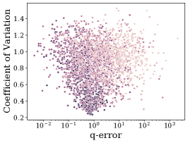
(a) $\mathsf{forest}$ NNGP

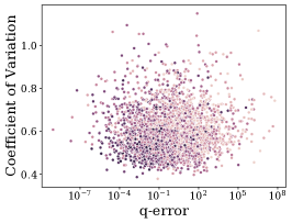
(b) $\mathsf{forest}$ DeepEns

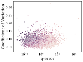
(c) $\mathsf{forest}$ BNN-MCD

(d) $\mathsf{TPC}$-$\mathsf{DS}$ NNGP

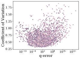
(e) $\mathsf{TPC}$-$\mathsf{DS}$ DeepEns

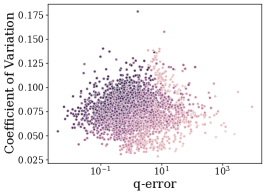
(f) $\mathsf{TPC}$-$\mathsf{DS}$ BNN-MCD

Figure 5. Visualization of Estimation Uncertainty

We have implemented above two techniques for the lightweight neural network estimator (DBLP:journals/pvldb/DuttWNKNC19, ), as DeepEns and BNN-MCD respectively. The estimator is a two-layer multilayer perceptron with 512 hidden units. The DeepEns ensembles 5 estimators and BNN-MCD uses a dropout probability of 0.5 and 2,000 forward passes for the prediction.

Fig. 5 visualizes the uncertainty and the $\mathsf{q}$-$\mathsf{error}$ for thousands of queries on $\mathsf{forest}$ and $\mathsf{TPC}$-$\mathsf{DS}$, where the points denote testing queries. The uncertainty is represented by coefficient of variation, which is the standard deviation normalized by the mean, to quantify the dispersion of the predictive distribution. Ideally, the uncertainty should be highly correlated with the prediction error. That is, the larger the $\mathsf{q}$-$\mathsf{error}$, the larger the uncertainty. NNGP estimator shows such behavior. For the queries with larger $\mathsf{q}$-$\mathsf{error}$, their coefficient of variation of NNGP estimator is large in Fig. 5(a) and Fig. 5(d), where the scatter plots are in a V-shape. For DeepEns and BNN-MCD, this V-shape distribution is not obvious. The flat bottom in the scatter plots indicates the estimators are still over-confident on some queries whose $\mathsf{q}$-$\mathsf{error}$ is far away from 1.0. Furthermore, we also observe that DeepEns still has a relative worse performance w.r.t. prediction accuracy, compared with NNGP and BNN-MCD. And BNN-MCD faces the risk of unstable training as the variational inference aims to optimize a lower bound of the original training loss. All the three estimators make some conservative predictions in the sense that the actual $\mathsf{q}$-$\mathsf{error}$ is small whereas the uncertainty is large. It reflects the fact that all of them are possible to process queries out-of-distribution, via different smoothing techniques on their prediction.

In terms of efficiency, DeepEns needs to train and maintain multiple neural networks explicitly, and BNN-MCD needs to conduct a large number of forward passes in the testing phase. It is impractical to deploy these two techniques on high-end DL estimators, (e.g., the Tree LSTM estimator (DBLP:journals/pvldb/SunL19, )) in a DBMS. In section 6, we show that the training and prediction of NNGP are faster than wide neural network, thus is faster than the DeepEns and BNN-MCD counterparts.

6. Experimental Studies

In this section, we give the test setting (section 6.1), and report the extensive experiments in the following facets: ① Compare the accuracy of NNGP estimator with state-of-the-art ML/DL estimators (section 6.2). ② Test the training and prediction efficiency of NNGP estimator and verify it is a lightweight DL-based estimator (section 6.3). ④ Validate the robustness of NNGP estimation regarding small number of training queries and unbalanced workloads (section 6.4) ③ Study the application of the uncertainty that NNGP provides in active learning, which all the DL-based estimators do not support (section 6.5).

6.1. Experimental Setup

Baseline Approaches. To comprehensively evaluate the effectiveness and efficiency of NNGP estimator, we compare it with 8 estimators including 5 query-driven learned estimators, 2 data-driven learned estimators and 1 traditional estimator as follows. ➊ Neural Network (NN) (DBLP:journals/pvldb/DuttWNKNC19, ) is the standard fully-connected neural network with $\mathsf{ReLU}$ activation. ➋ Gradient Boosting Decision Tree (GBDT) (DBLP:journals/pvldb/DuttWNKNC19, ; dutt2020efficiently, ) is the ensembling decision regression trees by gradient boosting. ➌ Multi-set Convolutional Neural Network (MSCN) (DBLP:conf/cidr/KipfKRLBK19, ) firstly embeds the table set, join set and predicate set by 3 separate multilayer perceptrons as the set convolutions, respectively, and then concatenate the 3 embeddings to a long vector and feed it into a final output network. ➍ Tree LSTM (TLSTM) (DBLP:journals/pvldb/SunL19, ) is a high-end DL model originally designed for cost and cardinality estimation, by taking tree-structured query plans as its input. It is composed of three stacked layers, the embedding layer, representation layer and estimation layer. The embedding layer embeds operations (join and table scan), predicates, metadata of leaf nodes of the plan tree into vector representations. The embedding layer aggregates the representation of each node on the tree in a bottom-up fashion by Tree-Structured LSTM (DBLP:conf/acl/TaiSM15, ). The estimation layer is a fully-connected neural network with $\mathsf{sigmoid}$ activations that finally outputs the predictions. A detailed formulation of the model can be found in (DBLP:journals/pvldb/SunL19, ). ➎ DeepDB (DBLP:journals/pvldb/HilprechtSKMKB20, ) (DeepDB) is an unsupervised learning, data-driven estimator that uses Relational Sum-Product Network (RSPN) (DBLP:conf/aaai/NathD15, ) to model the joint distribution of a relation. To support join queries, an ensemble of RSPNs or a joint RSPN is built, and the choice is based on independent test on the relations. SQL queries are complied into probabilistic queries on the RSPN. ➏ Naru (DBLP:journals/pvldb/YangLKWDCAHKS19, )/NeuroCard (DBLP:journals/corr/abs-2006-08109, ) (NeuroCard) factorizes the joint distribution into conditional distributions and adopts deep autoregressive models such as MADE (DBLP:conf/icml/GermainGML15, ) or Transformer (DBLP:conf/nips/VaswaniSPUJGKP17, ) to approximate the joint distribution. NeuroCard further extends Naru to support full outer joins. To predict the cardinalities, progressive sampling is conducted over the density model. ➐ PostgreSQL estimator (Postgres) is a build-in statistical estimator. Estimated cardinality is obtained from the EXPLAIN command of PostgreSQL. ➑ Gaussian Process with radial basis kernel function (GP-RBF) is compared as a typical GP baseline. All the above learned estimators only support PK/FK joins.

Implementation and Settings. The NNGP estimator is built on Neural Tangents (neuraltangents2020, ), which is based on Google JAX  (jax2018github, ). The empirical zero-mean Gaussian prior is imposed on the weights of neural networks and $\mathsf{ReLU}$ is used as the nonlinear activation, leading to a closed-form kernel function for Bayesian inference. There is no extra cost paid for NNGP hyper-parameters tuning. GBDT estimator is implemented by XGBoost  (caDBLP:conf/kdd/ChenG16, ) and a tree ensemble contains 32 trees. GP-RBF is implemented by the exact GP regressor of scikit-learn. For NeuroCard, we follow all the hyper-parameter configurations in its implementation based on MADE as the deep autoregressive model. NN, MSCN, and TLSTM estimators are implemented by PyTorch 1.6  (pytorch, ). We use the Adam optimizer with a decaying learning rate to train these models. For different datasets, the main hyper-parameters for training are tuned in their empirical range: learning rate $\in[10^{-3},10^{-4}]$, epochs $\in\{50,80,100\}$, mini-batch size $\in\{16,32,64\}$, L2 penalty of Adam $\in[10^{-3},10^{-5}]$. For NN, GBDT, GP-RBF and NNGP, their encodings of input are same, as the introduction in section 2. Other models have their own input encoding due to their specific model design. Particularly, as TLSTM takes a tree-structured plan as input, we generate a left-deep tree for each join query following a total order of the relations. Since we only perform one task of cardinality estimation, one-hot physical operator encoding is simplified to the corresponding one-hot logical operator encoding. Both training and prediction are performed on a Linux server with 32 Intel(R) Xeon(R) Silver 4215 CPUs and 128G RAM.

Table 2. Query Sets

Type	Dataset	# Queries	# Select/Join Cond.	Range of $c(q)$
Single Rel.	$\mathsf{forest}$	18,000	{2, $\cdots$, 10}	$[10^{0},10^{6}]$
Single Rel.	$\mathsf{higgs}$	12,000	{2, $\cdots$, 7}	$[10^{0},10^{8}]$
Join	$\mathsf{TPC}$-$\mathsf{H}$	16,000	{0, 1, 2, 3}	$[10^{0},10^{7}]$
Join	$\mathsf{TPC}$-$\mathsf{DS}$	15,000	{0, 1, 2, 3, 4}	$[10^{0},10^{7}]$

Datasets. We use 4 relational datasets, 2 for single relation range queries, 2 for multi-relation join queries. $\mathsf{forest}$ (Dua:2019, ) originally contains 54 attributes of forest cover type. Following (DBLP:journals/pvldb/DuttWNKNC19, ; DBLP:journals/vldb/GunopulosKTD05, ), we use the first 10 numerical attributes. The relation has about 581K of rows. $\mathsf{higgs}$ (Dua:2019, ) is a physical dataset contains 7 high-level kinematic attributes of particles, collected by detectors and post-processed by scientific functions. The relation has 11M rows. $\mathsf{TPC}$-$\mathsf{H}$ (1 GB). We use the relations supplier, orders, part and lineitem. There are 3 PK/FK join conditions. $\mathsf{TPC}$-$\mathsf{DS}$ (2 GB). We use the relations store, item, customer and promotion, store-sales, where store-sales is the factual relation and others are the dimensional relations. There are 5 PK/FK join conditions and the schema has a cycle.

Queries. We construct large query workloads in the following way. For single relation $\mathsf{forest}$ and $\mathsf{higgs}$, we generate query sets with the number of select conditions varying from 2 to $D$ where $D$ is the number of attributes, and generate 2,000 queries for each subset. To generate a query of $d$ selection conditions, first we uniformly sample $d$ attributes from all the $D$ attributes, then uniformly sample each attribute by the data-centric distribution following  (DBLP:journals/pvldb/DuttWNKNC19, ). For join queries, we test and report the existing baselines supported query type, i.e., PK/FK join without selection conditions on the join attributes. We generate query sets with the number of PK/FK joins, t, varying from 0 to $|T|-1$, where $|T|$ is the number of involved relations. To generate a query of $t~{}(t>0)$ joins, firstly a starting relation is uniformly sampled, then the query is constructed by traversing from the starting relation over the join graph in $t$ steps. Here, for each relation of the sampled join query, additional selection conditions are drawn independently. For each $t$, 4,000 and 3,000 queries are generated for $\mathsf{TPC}$-$\mathsf{H}$ and $\mathsf{TPC}$-$\mathsf{DS}$, respectively. We only preserve unique queries with nonzero cardinality. Table 2 summarizes the 4 corresponding query sets.

6.2. Accuracy

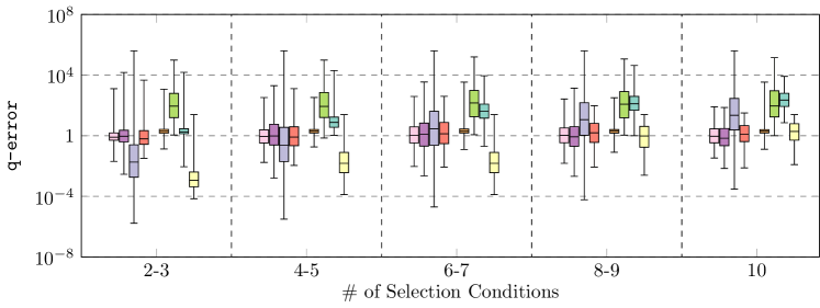
(a) $\mathsf{forest}$

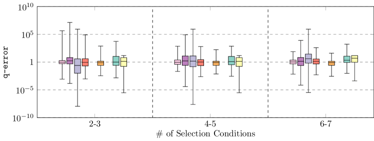
(b) $\mathsf{higgs}$

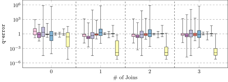
(c) $\mathsf{TPC}$-$\mathsf{H}$

(d) $\mathsf{TPC}$-$\mathsf{DS}$

Figure 6. Query Evaluation Accuracy

We investigate the estimation accuracy of NNGP estimator. For the query-centric approaches, i.e., NNGP, NN, GBDT, MSCN, TLSTM and GP-RBF, we split the queries into 60% for training, 20% for validation and 20% for testing. The split is conducted by stratified sampling on the subsets with different numbers of selection/join conditions.

Fig. 6 presents the statistical distribution of $\mathsf{q}$-$\mathsf{error}$ of NNGP compared with the 8 baselines. In general, NNGP, MSCN and DeepDB are the top three best performed estimators. There is no an overall best estimator that consistently outperforms others under all the test circumstances. Due to the infinite wide hidden layer, the performance of NNGP consistently surpasses the finite wide NN. The performance advantage of NNGP is mainly reflected in queries of single relation (Fig. 6(a), 6(b)), and the 25%-75% quantile of $\mathsf{q}$-$\mathsf{error}$ is within 1.5. For the join queries (Fig. 6(c), 6(d)), we speculate the join encoding and the multilayer perceptrons based kernel of NNGP are simple to model the complex join queries. In contrast, the performance advantage of MSCN is reflected in the join queries rather than queries on single relation. Due to satisfaction the behavior logics, DeepDB achieves a promising 25%-75% quantile of $\mathsf{q}$-$\mathsf{error}$. However, we observe that there are many over/underestimated queries for $\mathsf{forest}$ (Fig. 6(a)) and $\mathsf{TPC}$-$\mathsf{DS}$ (Fig. 6(d)), as the model would factorize intertwined attributes under the conditional independent assumption.

We discuss other baseline approaches. Although TLSTM is a high-end DL estimator with complex layers, its performance is not promising for a sole cardinality estimation task. We speculate TLSTM is mainly applicable for real cost estimation tasks when more features about the physical operators and meta-data of the physical database are fed into the model. Its original implementation learns TLSTM by multi-task learning for the physical cost and the cardinality. However, the tree-structured plan directly influences the physical cost but not the cardinality. The simple GP baseline, GP-RBF, underfits the training queries, and therefore it cannot be used as a cardinality estimator. It indicates the representation learning provided by DL is critical for a complicated learning task. Postgres uses single column statistics and assumes the columns are independent. This conventional statistical approach performs well on the benchmark $\mathsf{TPC}$-$\mathsf{H}$ but leads to large estimation bias on other datasets, particularly for complex queries.

6.3. Efficiency

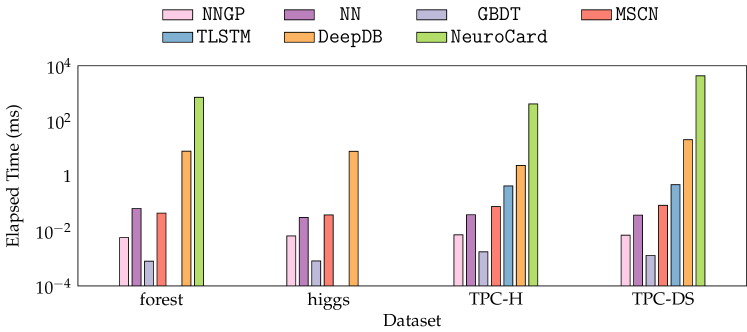
Figure 7. Query Evaluation Latency (ms)

We compare the prediction time of NNGP estimators with the baseline approaches. Fig. 7 presents the average elapsed time of the whole test query set on our 32-core CPU. In general, the lightweight GBDT estimator achieves the fastest prediction and our NNGP estimator is the second best. XGBoost is a well-optimized learning system for GBDT. The inference of NNGP is a linear combination of the ground-truth cardinalities, where the weights are the closed-form kernels of Eq. (18). The prediction of DeepDB is 2-3 orders of magnitude slower than that of supervised learning approaches. DeepDB needs to perform a bottom-up pass on the tree-structured deep sum-product network. Estimation on NeuroCard is quite slow as one query needs thousands of sampling on the model to perform a Monte Carlo integration. We noticed that in its original paper (DBLP:journals/corr/abs-2006-08109, ), the GPU executed prediction is up to 2 orders of magnitude faster than our CPU execution. That means GPU acceleration is necessary to employ NeuroCard as an estimator available for DBMS. However, NeuroCard also consumes large GPU memory. Training on $\mathsf{forest}$ is out of memory on a 16GB Nvidia V100. In terms of easy use for DBMS, lightweight estimators like our NNGP have a great advantage. For NNGP, NN and GBDT, the prediction time for queries with different number of selection/join conditions are equal, as the input vectors are of equal length. For other estimators, the more complex the query, the longer the prediction time. The prediction time of DeepDB and NeuroCard is also related to the database schema. In general, complex schema incurs a larger model and longer prediction time.

Scalability of Training. We test the scalability of NNGP estimator in the facets of training time and memory usage, comparing with the top-2 lightweight models NN and GBDT. As the the number of queries increases linearly, Fig. 8(a), 8(c), 8(e) and 8(g) show the training time on CPUs, where training an NN takes tens to hundreds seconds while training GBDT or NNGP only takes less than 3 seconds. Although the training complexity of NNGP is $O(N^{3})$, the exact Bayesian inference is boosted by highly paralleled basic linear algebra operations. The time complexity of NN is $O(TNd^{2}h)$, where $T$, $d$, and $h$ are the number of iterations/epochs, dimension of input and the number of neurons in the hidden layer. Extra overhead is involved in the forward/backward propagation. Fig. 8(b), 8(d), 8(f) and 8(h) show the peak memory usage monitored in the training phase. Compared to NN and GBDT, NNGP needs more memory to persist the kernel matrix, which is quadratic to the number of training queries. Fortunately, as we will show in section 6.4, as a nonparametric model, NNGP already achieves satisfying and robust performance under a small volume of training data. It is worth noting that all the other estimators are more time and memory consuming than the two-layer NN. Given the same epoch, training of MSCN is roughly constant time slower than that of NN and training of TLSTM is even much slower than that of MSCN and NN. For the data-driven estimators, DeepDB and NeuroCard, the resources consumed are directly determined by the scale of the input relations. Among all the learned estimators, the most consuming is NeuroCard, where training on the large dataset $\mathsf{higgs}$ is failed within 72 hours.

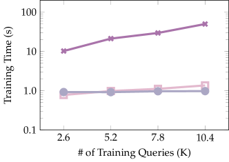
(a) $\mathsf{forest}$

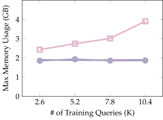
(b) $\mathsf{forest}$

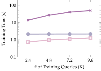
(c) $\mathsf{higgs}$

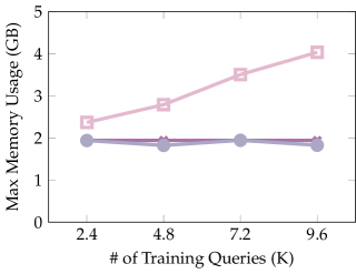
(d) $\mathsf{higgs}$

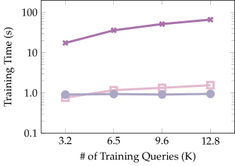
(e) $\mathsf{TPC}$-$\mathsf{H}$

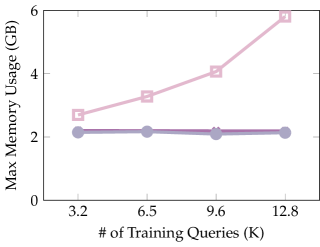
(f) $\mathsf{TPC}$-$\mathsf{H}$

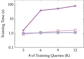
(g) $\mathsf{TPC}$-$\mathsf{DS}$

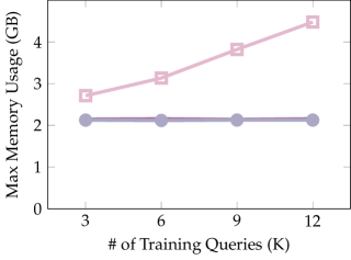
(h) $\mathsf{TPC}$-$\mathsf{DS}$

Figure 8. Training Time & Memory Usage

6.4. Robustness to Workload Shifts

To study the robustness of NNGP estimator, we train different models independently over various training workloads of $\mathsf{forest}$ and $\mathsf{TPC}$-$\mathsf{H}$, and test the models on split fixed test query sets, i.e., 20% of the whole query sets. The test queries are evenly distributed on the number of selection conditions for $\mathsf{forest}$ or the number of join conditions for $\mathsf{TPC}$-$\mathsf{H}$. To generate various training workloads, first, we control the total number of training queries to $1,000$, $2,000$, $4,000$, $8,000$, respectively, where the queries with different numbers of selection/join conditions are evenly distributed, and the result is shown in Fig. 9(a) and 9(c). Second, the total number of training queries is fixed to 40% of the whole queries, and the fraction of queries with less/more selection or join conditions is set within {2:8, 4:6, 6:4, 8:2}. $\mathsf{forest}$ queries with 2-5 selection conditions are regarded as less conditions queries while others are more conditions. $\mathsf{TPC}$-$\mathsf{H}$ queries with 0-1 joins are regarded as less conditions queries while others are more conditions. The testing results on the fixed 20% test queries are shown in Fig. 9(b) and 9(d).

In general, the key observation is that the NNGP estimator performs supremely robust on various workloads, regardless of the number of training queries and the fraction of different queries. In Fig. 9(a) and 9(c), even though there are only $1,000$ training queries, the $\mathsf{q}$-$\mathsf{error}$ statistics of NNGP varies within one order of magnitude compared with the model with $8,000$ training queries, and even better than NN with $8,000$ training queries. In contrast, due to overfitting, the $\mathsf{q}$-$\mathsf{error}$ of its counterpart NN is degenerated drastically in the scenario of fewer training queries, which is up to $10^{10}$. As the fraction of queries with less/more selection or join conditions shifts in Fig. 9(b) or Fig. 9(d), respectively, the performance of NNGP also oscillates slightly. As a nonparametric model, GBDT is relatively more robust than NN but has a larger $\mathsf{q}$-$\mathsf{error}$. We notice that GBDT underfits on $\mathsf{forest}$, whose prediction has a large bias on the test queries and even on the training queries. In the experiments, we also observe that the performance of NN estimator is not stable during multiple runs, which is influenced by parameter initialization and stochastic optimization.

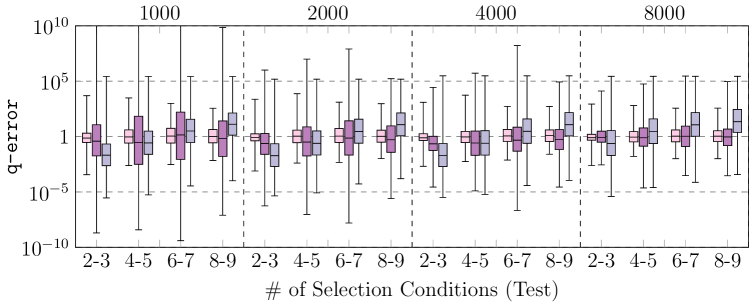
(a) Varying the number of training queries for $\mathsf{forest}$

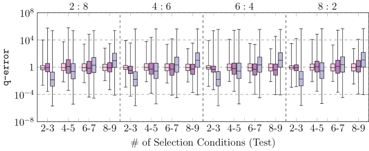
(b) Varying the fraction of predicate size for $\mathsf{forest}$

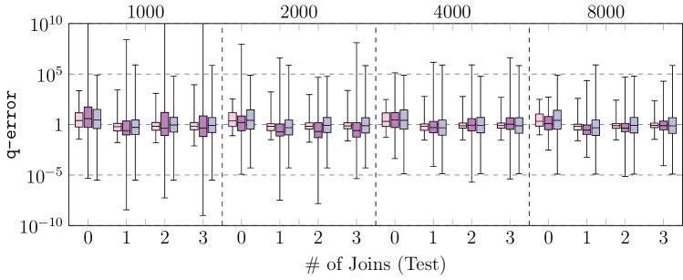
(c) Varying the number of training queries for $\mathsf{TPC}$-$\mathsf{H}$

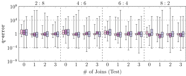
(d) Varying the fraction of join size for $\mathsf{TPC}$-$\mathsf{H}$

Figure 9. Robustness to Various Training Workloads

6.5. Uncertainty for Active Learning

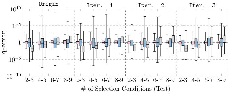
(a) $\mathsf{forest}$

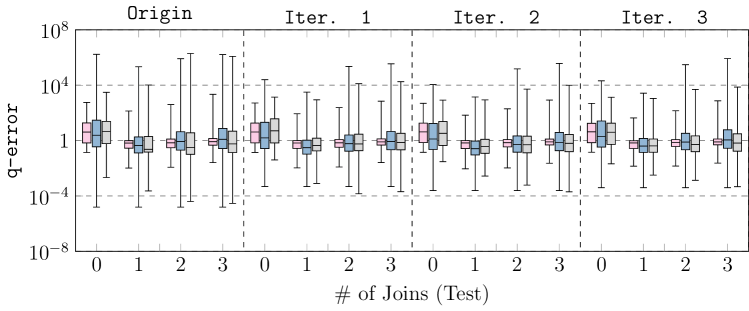
(b) $\mathsf{TPC}$-$\mathsf{H}$

Figure 10. $\mathsf{q}$-$\mathsf{error}$ of 3 Iterations of Active Learning

Table 3. mean-squared-error (MSE) on test queries

MSE	Estimator	Origin	Iter. 1	Iter. 2	Iter. 3
$\mathsf{forest}$	NNGP	6.27	5.79	5.65	5.50
	DeepEns	45.43	38.00	35.26	33.50
	BNN-MCD	36.18	33.63	34.87	34.80
$\mathsf{TPC}$-$\mathsf{H}$	NNGP	5.30	5.13	5.02	4.95
	DeepEns	14.14	11.29	10.87	10.49
	BNN-MCD	16.78	11.45	11.35	11.53

Finally, we investigate leveraging the predictive uncertainty to improve the model explicitly by active learning. The key step of active learning is to select a set of informative test data to enrich the original training data and update the model (DBLP:series/synthesis/2012Settles, ). The predictive uncertainty, as the model’s belief on its prediction, is an efficient and effective selection criterion. The corresponding active learning algorithm, a.k.a., uncertainty sampling (DBLP:conf/icml/LewisC94, ), is to sample from the region of the data which has the most uncertainty regarding the current model, request the ground truth for these test data and retrain/update the model by original and added data. This process is repeated for several iterations under a specified stop condition, e.g., a given iteration number or sampling budget. As the existing DL-based estimators do not deliver the predictive uncertainty, we used the two uncertainty-aware DL-based estimators introduced in section 5, DeepEns and BNN-MCD, as the baselines.

To conduct active learning, the entire queries are split into 40% for training an original base estimator, 20% for testing and 40% as a selection pool. The base DeepEns (5 NN estimators for the ensemble) and BNN-MCD are trained by 50 epochs. We apply 3 iterations of uncertainty sampling where each iteration 1,000 queries are drawn without replacement regarding the coefficient of variation. DeepEns and BNN-MCD are updated on their base model, and NNGP is retrained from scratch. Table 3 presents the mean-squared-error (MSE) (Eq. (21)) for the base model and those after the 3 iterations, on the test query set. NNGP and the two DL baselines are able to improve themselves introspectively via uncertainty-based active learning. Among them NNGP achieves the lowest test MSE. The MSE of NNGP and DeepEns are consistently reduced in the 3 iterations although the MSE of NNGP is already small. A close observation on the prediction accuracy of different $\mathsf{forest}$ and $\mathsf{TPC}$-$\mathsf{H}$ queries is shown in Fig. 10. Due to the neural network nature, the performance of BNN-MCD and DeepEns improves significantly as more queries are incorporated into the training set. As the test MSE of origin NNGP is small, its $\mathsf{q}$-$\mathsf{error}$ reduction is not obvious compared with BNN-MCD and DeepEns. But we still can observe an improvement on the queries with 2-3 joins in Fig. 10(b). The model updating has marginal effect for all the three estimators.

7. Related Work

Classical Cardinality Estimators. Cardinality/Selectively estimation of relational queries is studied over decades in the database area. Early approaches propose multi-dimensional histograms to represent the joint probability distribution (DBLP:conf/vldb/PoosalaI97, ; DBLP:journals/vldb/GunopulosKTD05, ; DBLP:conf/sigmod/PoosalaIHS96, ), where the assumption of attribute value independence is not necessary to be held. For join queries, join sampling algorithms (haas1999ripple, ; DBLP:conf/sigmod/0001WYZ16, ; DBLP:conf/sigmod/CaiBS19, ; DBLP:conf/sigmod/ZhaoC0HY18, ) are designed, which can be used to approximate cardinality and query results. These approaches face the risk of sampling failure in the intermediate join step, when the data distribution is complex. (DBLP:conf/sigmod/GetoorTK01, ; DBLP:journals/pvldb/TzoumasDJ11, ) use Bayesian Network to estimate cardinality by modeling the joint probability distribution of all the attributes. Structural learning is needed to explore a well-structured DAG to represent potential conditional independence of attribute. Note Bayesian Network is different from Bayesian neural network. The former is a probabilistic graphical model based on the conditional independence assumption whereas the latter is the Bayesian DL model.

ML/DL for Cardinality Estimation and AQP. ML/DL models are exploited to perform cardinality estimation and AQP for RDBMS. We briefly review ML/DL approaches in Table 1. DBEst (DBLP:conf/sigmod/MaT19, ) builds kernel density estimation (KDE) models and tree-based regressors to conduct AQP. DeepDB (DBLP:journals/pvldb/HilprechtSKMKB20, ) adopts Sum-Product Networks (SPNs) to learn the joint probability distribution of attributes. An SQL query is complied to a product of expectations or probability queries on the SPNs, where the product is based on independence of the attributes. (DBLP:conf/icde/Thirumuruganathan20, ) uses deep generative model, e.g., Variational Autoencoder (VAE) to model the joint probability distribution of attributes, which only support analytical aggregate query on a single table. (DBLP:journals/pvldb/KieferHBM17, ) estimates multivariate probability distributions of a relation to perform cardinality estimation by KDE. Multiple joins can be estimated by building the KDE estimator on pre-computed join result or an estimation formula that leverages samples from the multiple relations as well as the models. Deep autoregressive model, e.g., Masked Autoencoder (MADE), is also adopted to learn the joint probability distribution (DBLP:journals/pvldb/YangLKWDCAHKS19, ; DBLP:conf/sigmod/HasanTAK020, ), which decomposes the joint distribution to a product of conditional distributions. Kipf et al. propose a multi-set convolutional neural network (MSCN) to express query features using sets (DBLP:conf/cidr/KipfKRLBK19, ). Anshuman et al. (DBLP:journals/pvldb/DuttWNKNC19, ) use MLP and tree-based regressor to express multiple attributes range queries. Sun et al. (DBLP:journals/pvldb/SunL19, ) extract the features of physical query plan by Tree LSTM to estimate the query execution cost as well as the cardinality.

ML/DL for Databases. In recent years, with the development of ML/DL techniques, ML/DL models are exploited to support multiple database applications. Various types of ML/DL models serve as a cost estimator of algorithms or query plans, which are to support applications of data partitioning (DBLP:conf/sigmod/FanJLLLXYYZ20, ), index recommendation (DBLP:conf/sigmod/DingDM0CN19, ) and concurrency control (DBLP:journals/pvldb/ZhouSLF20, ). (DBLP:conf/sigmod/NathanDAK20, ; DBLP:conf/sigmod/KraskaBCDP18, ; DBLP:conf/sigmod/DingMYWDLZCGKLK20, ; DBLP:conf/sigmod/MarcusZK20, ) propose learned index structures, which learn a cumulative distribution function of the underlying data. (DBLP:journals/pvldb/MarcusNMZAKPT19, ; DBLP:journals/corr/abs-1808-03196, ; DBLP:conf/sigmod/MarcusZK20, ) design end-to-end learning-based query optimizers where (DBLP:journals/pvldb/MarcusNMZAKPT19, ; DBLP:journals/corr/abs-1808-03196, ) optimize the binary join order and (DBLP:conf/sigmod/MarcusZK20, ) generates the physical plans. Their approaches reformulate the dynamical programming problem of query optimization to Markov Decision Process and adopt different reinforcement learning (RL) algorithms to learn neural network models as the optimizer. (DBLP:conf/sigmod/AkenPGZ17, ; DBLP:conf/sigmod/ZhangLZLXCXWCLR19, ; DBLP:conf/sigmod/KunjirB20, ; DBLP:journals/pvldb/DuanTB09, ) adopt ML/DL to tune the database configurations, where GP-based Bayesian optimization and RL algorithms are used respectively to conduct an online tuning in (DBLP:conf/sigmod/AkenPGZ17, ; DBLP:journals/pvldb/DuanTB09, ) and (DBLP:conf/sigmod/ZhangLZLXCXWCLR19, ; DBLP:conf/sigmod/KunjirB20, ). It is worth mentioning that this paper is the first exploration of Bayesian DL in the database area.

8. Conclusion

In this paper, we explore a new simple yet effective NNGP estimator to estimate cardinality of SQL queries. We compare it with 7 baseline estimators over 4 relational datasets. In terms of accuracy, NNGP is one of the top-3 estimators, and performs best in many cases. In terms of efficiency of training, NNGP is 1-2 orders faster than the baseline estimators except GBDT. GBDT is marginally more efficient than NNGP but has a low prediction accuracy. In terms of uncertainty, NNGP can consistently improve its accuracy by uncertainty sampling via active learning, whereas BNN cannot do so. And it achieves a much smaller prediction error comparing to Deep Ensemble and BNN. In addition, NNGP is supremely robust on various workloads, and can be learned with much fewer training queries. Our source code is public available in https://github.com/Kangfei/NNGP.

References

- [1] Pytorch. https://github.com/pytorch/pytorch.
- [2] D. V. Aken, A. Pavlo, G. J. Gordon, and B. Zhang. Automatic database management system tuning through large-scale machine learning. In Proc. SIGMOD’17, pages 1009–1024, 2017.
- [3] C. M. Bishop. Pattern recognition and machine learning, 5th Edition. Information science and statistics. Springer, 2007.
- [4] J. Bradbury, R. Frostig, P. Hawkins, M. J. Johnson, C. Leary, D. Maclaurin, G. Necula, A. Paszke, J. VanderPlas, S. Wanderman-Milne, and Q. Zhang. JAX: composable transformations of Python+NumPy programs, 2018.
- [5] W. Cai, M. Balazinska, and D. Suciu. Pessimistic cardinality estimation: Tighter upper bounds for intermediate join cardinalities. In Proc. SIGMOD’19, pages 18–35, 2019.
- [6] J. Chen, M. Stern, M. J. Wainwright, and M. I. Jordan. Kernel feature selection via conditional covariance minimization. In Proc. NIPS’19, pages 6946–6955, 2017.
- [7] T. Chen and C. Guestrin. Xgboost: A scalable tree boosting system. In Proc. SIGKDD’16, pages 785–794, 2016.
- [8] Y. Cho and L. K. Saul. Kernel methods for deep learning. In Proc. NIPS’09, pages 342–350, 2009.
- [9] B. Ding, S. Das, R. Marcus, W. Wu, S. Chaudhuri, and V. R. Narasayya. AI meets AI: leveraging query executions to improve index recommendations. In Proc. SIGMOD’19, pages 1241–1258, 2019.
- [10] J. Ding, U. F. Minhas, J. Yu, C. Wang, J. Do, Y. Li, H. Zhang, B. Chandramouli, J. Gehrke, D. Kossmann, D. B. Lomet, and T. Kraska. ALEX: an updatable adaptive learned index. In Proc. SIGMOD’20, pages 969–984, 2020.
- [11] D. Dua and C. Graff. UCI machine learning repository, 2017.
- [12] S. Duan, V. Thummala, and S. Babu. Tuning database configuration parameters with ituned. Proc. VLDB Endow., 2(1):1246–1257.
- [13] A. Dutt, C. Wang, V. Narasayya, and S. Chaudhuri. Efficiently approximating selectivity functions using low overhead regression models. Proc. VLDB Endow., 13(12):2215–2228, 2020.
- [14] A. Dutt, C. Wang, A. Nazi, S. Kandula, V. R. Narasayya, and S. Chaudhuri. Selectivity estimation for range predicates using lightweight models. Proc. VLDB, 12(9):1044–1057, 2019.
- [15] W. Fan, R. Jin, M. Liu, P. Lu, X. Luo, R. Xu, Q. Yin, W. Yu, and J. Zhou. Application driven graph partitioning. In Proc. SIGMOD’20, pages 1765–1779, 2020.
- [16] Y. Gal and Z. Ghahramani. Bayesian convolutional neural networks with bernoulli approximate variational inference. CoRR, abs/1506.02158, 2015.
- [17] Y. Gal and Z. Ghahramani. Dropout as a bayesian approximation: Representing model uncertainty in deep learning. In Proc. ICML’16, volume 48, pages 1050–1059, 2016.
- [18] A. Garriga-Alonso, C. E. Rasmussen, and L. Aitchison. Deep convolutional networks as shallow gaussian processes. In Proc. ICLR’19, 2019.
- [19] M. Germain, K. Gregor, I. Murray, and H. Larochelle. MADE: masked autoencoder for distribution estimation. In Proc. ICML’15, volume 37, pages 881–889, 2015.
- [20] L. Getoor, B. Taskar, and D. Koller. Selectivity estimation using probabilistic models. In Proc. SIGMOD’01, pages 461–472, 2001.
- [21] D. Gunopulos, G. Kollios, V. J. Tsotras, and C. Domeniconi. Selectivity estimators for multidimensional range queries over real attributes. VLDB J., 14(2):137–154, 2005.
- [22] C. Guo, G. Pleiss, Y. Sun, and K. Q. Weinberger. On calibration of modern neural networks. In Proc. ICML’17, volume 70, pages 1321–1330. PMLR, 2017.
- [23] P. J. Haas and J. M. Hellerstein. Ripple joins for online aggregation. ACM SIGMOD Record, 28(2):287–298, 1999.
- [24] S. Hasan, S. Thirumuruganathan, J. Augustine, N. Koudas, and G. Das. Deep learning models for selectivity estimation of multi-attribute queries. In Proc. SIGMOD’20, pages 1035–1050, 2020.
- [25] B. Hilprecht, A. Schmidt, M. Kulessa, A. Molina, K. Kersting, and C. Binnig. Deepdb: Learn from data, not from queries! Proc. VLDB, 13(7):992–1005, 2020.
- [26] K. Hornik. Approximation capabilities of multilayer feedforward networks. Neural Networks, 4(2):251–257, 1991.
- [27] K. Hornik, M. B. Stinchcombe, and H. White. Universal approximation of an unknown mapping and its derivatives using multilayer feedforward networks. Neural Networks, 3(5):551–560, 1990.
- [28] J. Hron, Y. Bahri, J. Sohl-Dickstein, and R. Novak. Infinite attention: NNGP and NTK for deep attention networks. In Proc. ICML’20, volume 119, pages 4376–4386. PMLR, 2020.
- [29] J. Hu, J. Shen, B. Yang, and L. Shao. Infinitely wide graph convolutional networks: Semi-supervised learning via gaussian processes. CoRR, abs/2002.12168, 2020.
- [30] F. Hutter, L. Kotthoff, and J. Vanschoren. Automated machine learning: methods, systems, challenges. Springer Nature, 2019.
- [31] M. Kiefer, M. Heimel, S. Breß, and V. Markl. Estimating join selectivities using bandwidth-optimized kernel density models. Proc. VLDB, 10(13):2085–2096, 2017.
- [32] A. Kipf, T. Kipf, B. Radke, V. Leis, P. A. Boncz, and A. Kemper. Learned cardinalities: Estimating correlated joins with deep learning. In Proc. CIDR’19, 2019.
- [33] T. Kraska, A. Beutel, E. H. Chi, J. Dean, and N. Polyzotis. The case for learned index structures. In Proc. SIGMOD’18, pages 489–504, 2018.
- [34] S. Krishnan, Z. Yang, K. Goldberg, J. M. Hellerstein, and I. Stoica. Learning to optimize join queries with deep reinforcement learning. CoRR, abs/1808.03196, 2018.
- [35] M. Kunjir and S. Babu. Black or white? how to develop an autotuner for memory-based analytics. In Proc. SIGMOD’20, pages 1667–1683, 2020.
- [36] B. Lakshminarayanan, A. Pritzel, and C. Blundell. Simple and scalable predictive uncertainty estimation using deep ensembles. In Proc. NIPS’17, pages 6402–6413, 2017.
- [37] H. K. Lee. Bayesian nonparametrics via neural networks. SIAM, 2004.
- [38] J. Lee, Y. Bahri, R. Novak, S. S. Schoenholz, J. Pennington, and J. Sohl-Dickstein. Deep neural networks as gaussian processes. In Proc. ICLR’18, 2018.
- [39] D. D. Lewis and J. Catlett. Heterogeneous uncertainty sampling for supervised learning. In Proc. ICML’94, pages 148–156, 1994.
- [40] F. Li, B. Wu, K. Yi, and Z. Zhao. Wander join: Online aggregation via random walks. In Proc. SIGMOD’16, pages 615–629, 2016.
- [41] X. Liang, A. J. Elmore, and S. Krishnan. Opportunistic view materialization with deep reinforcement learning. CoRR, abs/1903.01363, 2019.
- [42] Q. Ma and P. Triantafillou. Dbest: Revisiting approximate query processing engines with machine learning models. In Proc. SIGMOD’19, pages 1553–1570, 2019.
- [43] D. J. MacKay. Introduction to gaussian processes. NATO ASI series F computer and systems sciences, 168:133–166, 1998.
- [44] R. Marcus, E. Zhang, and T. Kraska. Cdfshop: Exploring and optimizing learned index structures. In Proc. SIGMOD’20, pages 2789–2792, 2020.
- [45] R. C. Marcus, P. Negi, H. Mao, C. Zhang, M. Alizadeh, T. Kraska, O. Papaemmanouil, and N. Tatbul. Neo: A learned query optimizer. Proc. VLDB Endow., 12(11):1705–1718, 2019.
- [46] A. Nath and P. M. Domingos. Learning relational sum-product networks. In Proc. AAAI’15, pages 2878–2886, 2015.
- [47] V. Nathan, J. Ding, M. Alizadeh, and T. Kraska. Learning multi-dimensional indexes. In Proc. SIGMOD’20, pages 985–1000, 2020.
- [48] R. M. Neal. Priors for infinite networks. In Bayesian Learning for Neural Networks, pages 29–53. Springer, 1996.
- [49] R. Novak, L. Xiao, Y. Bahri, J. Lee, G. Yang, J. Hron, D. A. Abolafia, J. Pennington, and J. Sohl-Dickstein. Bayesian deep convolutional networks with many channels are gaussian processes. In Proc. ICLR’19, 2019.
- [50] R. Novak, L. Xiao, J. Hron, J. Lee, A. A. Alemi, J. Sohl-Dickstein, and S. S. Schoenholz. Neural tangents: Fast and easy infinite neural networks in python. In Proc. ICLR’20, 2020.
- [51] V. Poosala and Y. E. Ioannidis. Selectivity estimation without the attribute value independence assumption. In Proc. VLDB’97, pages 486–495, 1997.
- [52] V. Poosala, Y. E. Ioannidis, P. J. Haas, and E. J. Shekita. Improved histograms for selectivity estimation of range predicates. In Proc. SIGMOD, pages 294–305, 1996.
- [53] C. E. Rasmussen and C. K. I. Williams. Gaussian processes for machine learning. MIT Press, 2006.
- [54] B. Settles. Active Learning. Synthesis Lectures on Artificial Intelligence and Machine Learning. Morgan & Claypool Publishers, 2012.
- [55] L. Song, A. J. Smola, A. Gretton, J. Bedo, and K. M. Borgwardt. Feature selection via dependence maximization. J. Mach. Learn. Res., 13:1393–1434, 2012.
- [56] J. Sun and G. Li. An end-to-end learning-based cost estimator. Proc. VLDB, 13(3):307–319, 2019.
- [57] K. S. Tai, R. Socher, and C. D. Manning. Improved semantic representations from tree-structured long short-term memory networks. In Proc. ACL’15, pages 1556–1566, 2015.
- [58] S. Thirumuruganathan, S. Hasan, N. Koudas, and G. Das. Approximate query processing for data exploration using deep generative models. In Proc. ICDE’20, pages 1309–1320, 2020.
- [59] K. Tzoumas, A. Deshpande, and C. S. Jensen. Lightweight graphical models for selectivity estimation without independence assumptions. Proc. VLDB Endow., 4(11):852–863, 2011.
- [60] A. Vaswani, N. Shazeer, N. Parmar, J. Uszkoreit, L. Jones, A. N. Gomez, L. Kaiser, and I. Polosukhin. Attention is all you need. In Proc. NeurIPS’17, pages 5998–6008, 2017.
- [61] H. Wang and D. Yeung. Towards bayesian deep learning: A framework and some existing methods. IEEE Trans. Knowl. Data Eng., 28(12):3395–3408, 2016.
- [62] X. Wang, C. Qu, W. Wu, J. Wang, and Q. Zhou. Are we ready for learned cardinality estimation? CoRR, abs/2012.06743, 2020.
- [63] C. K. I. Williams. Computation with infinite neural networks. Neural Comput., 10(5):1203–1216, 1998.
- [64] A. G. Wilson and P. Izmailov. Bayesian deep learning and a probabilistic perspective of generalization. In Proc. NeurIPS’20, 2020.
- [65] G. Yang. Wide feedforward or recurrent neural networks of any architecture are gaussian processes. In Proc. NeurIPS’19, pages 9947–9960, 2019.
- [66] Z. Yang, A. Kamsetty, S. Luan, E. Liang, Y. Duan, P. Chen, and I. Stoica. Neurocard: One cardinality estimator for all tables. Proc. VLDB Endow., 14(1):61–73, 2020.
- [67] Z. Yang, E. Liang, A. Kamsetty, C. Wu, Y. Duan, P. Chen, P. Abbeel, J. M. Hellerstein, S. Krishnan, and I. Stoica. Deep unsupervised cardinality estimation. Proc. VLDB, 13(3):279–292, 2019.
- [68] J. Zhang, Y. Liu, K. Zhou, G. Li, Z. Xiao, B. Cheng, J. Xing, Y. Wang, T. Cheng, L. Liu, M. Ran, and Z. Li. An end-to-end automatic cloud database tuning system using deep reinforcement learning. In Proc. SIGMOD’19, pages 415–432, 2019.
- [69] Z. Zhao, R. Christensen, F. Li, X. Hu, and K. Yi. Random sampling over joins revisited. In Proc. SIGMOD’18, pages 1525–1539, 2018.
- [70] X. Zhou, J. Sun, G. Li, and J. Feng. Query performance prediction for concurrent queries using graph embedding. Proc. VLDB Endow., 13(9):1416–1428, 2020.