Triangulating surfaces with bounded energy

Abstract.

We show that if a closed $C^{1}$-smooth surface in a Riemannian manifold has bounded Kolasinski–Menger energy, then it can be triangulated with triangles whose number is bounded by the energy and the area. Each of the triangles is an image of a subset of a plane under a diffeomorphism whose distortion is bounded by $\sqrt{2}$.

1. Introduction

It is a general principle in the theory of energies of manifolds that small energy implies uncomplicated topology. Probably, the first instance of this principle is Fáry–Milnor theorem [1, 6], stating that a knot in $\mathbb{R}^{3}$ whose total curvature is less than $4\pi$ is necessarily trivial.

For energies of curves in $\mathbb{R}^{3}$, there are bounds for the stick number and the average crossing number of a knot, see for example [7] and references therein.

For higher dimensional submanifolds some analogs exist, but are not abundant. The Fáry–Milnor theorem can be generalized to the case of surfaces [2]. Compactness results show that there are finitely many isotopy classes of submanifolds below some fixed energy level; see [5].

Motivated by [2], we give another bound on the complexity of a surface in $\mathbb{R}^{n}$ in terms of its energy. The topological complexity is measured by the minimal number of triangles in the triangulation. In particular, we bound the genus of a surface in terms of its energy. Actually, our result goes further. For a surface with given energy we construct a triangulation in such a way that each triangle is a graph of a function with bounded derivative and distortion. In this sense, the triangles in the triangulation are “almost flat”.

Noting that the energy $\mathcal{E}_{p}^{\ell}$ is introduced in Definition 2.1, we present now the main result of this paper,

Theorem 1.1.

Suppose $\Sigma\subset\mathbb{R}^{n}$ is a closed surface. Let $\ell\in\{1,\dots,4\}$ and $p>2\ell$. Suppose $\Sigma$ has energy $\mathcal{E}^{\ell}_{p}(\Sigma)=E<\infty$ and area $A$. Then $\Sigma$ can be triangulated with $C_{2}AE^{2/(p-2\ell)}$ triangles, where $C_{2}$ is a universal constant depending only on $p,\ell$ and $n$.

Each of the triangles is a graph of an open subset of a plane under a function whose derivative has norm bounded by $\sqrt{2}$ and whose distortion is bounded by $\sqrt{2}$.

Combining Theorem 1.1 with [3, Theorem 1.1] stating that the minimal number $T(g)$ of triangles in a triangulation of a closed surface of genus $g$ grows linearly with $g$, we obtain the following result.

Corollary 1.2.

There is a constant $C_{g}$ (depending on $\ell,n,p$) such that if $\Sigma\subset\mathbb{R}^{n}$ is a closed surface with $\mathcal{E}^{\ell}_{p}(\Sigma)=E<\infty$ and area $A$, where $p>2\ell$, then $g(\Sigma)\leq C_{g}AE^{2/(p-2\ell)}$.

The proof of Theorem 1.1 goes along the following lines. The key tool is the Regularity Theorem of [5], recalled as Theorem 2.4, which states that an $m$-dimensional submanifold with bounded energy can be covered by so-called graph patches, that is, subsets that are graphs of functions from subsets of $\mathbb{R}^{m}$ with bounded derivatives. The subsets in the cover have diameter controlled by the energy, that is, they are not too small. An immediate corollary of Theorem 2.4 is an Ahlfors like inequality, Proposition 2.8, controlling from both sides the volume of the part of a submanifold cut out by a ball whose center is on the submanifold.

Next, assuming $\Sigma$ is a surface of bounded energy and area, we find a cover of $\Sigma$ by balls of some radius $r$ (depending on the energy), such that each ball is a graph patch. We let the centers of the balls be $x_{1},\dots,x_{N}$. A simple topological argument in Subsection 3.1 allows us to control the number $N$ of the centers in terms of the energy and area of the surface.

To construct the triangulation, we connect all pairs $x_{i},x_{j}$, such that $||x_{i}-x_{j}||<4r$, by an arc $\gamma_{ij}$. The requirement on $\gamma_{ij}$, spelled out in Definition 3.5, is that the length $\ell(\gamma_{ij})$ be bounded by a constant times $||x_{i}-x_{j}||$. Unlike geodesics, two such curves can intersect at more than a single point. By a procedure called bigon removal we improve the collection of curves $\gamma_{ij}$ to obtain a concrete bound on the number of intersection points between them; see Lemma 3.19.

We let $\Sigma_{0}$ be the complement of $\bigcup\gamma_{ij}$ in $\Sigma$. The triangulation is constructed by cutting connected components of $\Sigma_{0}$ into triangles. A second technicality, and chronologically the first we deal with in this article, appears. We need to ensure that each connected component of $\Sigma_{0}$ is planar. We address this problem in Lemma 3.7. Given that lemma, we consider each component $C$ of $\Sigma_{0}$. As it is planar, we cut $C$ into triangles without adding new vertices. The number of triangles in the triangulation is estimated using the number of intersection points between curves $\gamma_{ij}$; see Corollary 4.8. The proof of Theorem 1.1 is summarized in Subsection 4.2.

Acknowledgements.

The paper is based on the Master thesis of the second named author under supervision of the first named author. The authors are grateful to Sławomir Kolasiński for fruitful discussions.

MB was supported by the Polish National Science Grant 2019/B/35/ST1/01120. MS was supported by the National Science Center grant 2016/22/E/ST1/00040.

2. Review of surface energies

In this section we recall definitions of surface energy. References include [4, 5, 8].

2.1. Discrete Menger energy for a submanifold in $\mathbb{R}^{n}$

For points $(x_{0},\dots,x_{m})$ in $\mathbb{R}^{n}$, we let $\Delta(x_{0},\dots,x_{m})$ denote the $m$-dimensional simplex spanned by $x_{0},\dots,x_{m}$ (the convex hull of these points). We define

$$\mathcal{K}(x_{0},\dots,x_{m})=\frac{1}{d^{m}}\operatorname{vol}_{m}\Delta(x_{0},\dots,x_{m}),$$

where $d$ is the diameter of $\Delta(x_{0},\dots,x_{m})$.

Suppose now $\Sigma\subset\mathbb{R}^{n}$ is a Lipshitz submanifold of dimension $m<n$. Let $\ell\in\{1,\dots,m+2\}$ and $p>0$.

Definition 2.1.

The Kolasinski-Menger energy of $\Sigma$ is the integral

(2.2) $$\mathcal{E}^{\ell}_{p}(\Sigma)=\int_{\Sigma^{\ell}}\sup_{x_{\ell},\dots,x_{m+2}\in\Sigma}\mathcal{K}(x_{0},\dots,x_{m+2})^{p}\,d\!\operatorname{vol}(\Sigma^{\ell}).$$

The integral is computed with respect to variables $x_{0},\dots,x_{\ell-1}$.

2.2. Graph patches

For $\alpha\in(0,1]$, we let $\mathcal{C}^{1,\alpha}_{m,n}$ denote the set of all compact smooth manifolds of dimension $m$, embedded $C^{1,\alpha}$-smoothly in $\mathbb{R}^{n}$. The following definition is taken from [5, Definition 1]

Definition 2.3 (Graph patches).

Suppose $R,L,d$ are real positive and $\alpha\in(0,1]$. The class $\mathcal{C}^{1,\alpha}_{m,n}(R,L,d)$ is the class of all $m$-dimensional submanifolds $\Sigma\subset\mathbb{R}^{n}$ such that:

1. $\Sigma\subset B(0,d)$ ;

2. for each $x\in\Sigma$, there exists a function $f_{x}\colon T_{x}\Sigma\to T_{x}\Sigma^{\perp}$ of class $C^{1,\alpha}$ with $f_{x}(0)=0$, $Df_{x}(0)=0$ and

   $$\Sigma\cap B(x,R)=(x+\operatorname{graph}(f_{x}))\cap B(x,R).$$

3. the function $f_{x}$ is Lipshitz with Lipshitz constant $1$ and $||Df_{x}(\xi)-Df_{x}(\eta)||\leq L|\xi-\eta|^{\alpha}$.

We quote now the following result

Theorem 2.4 ([5, Regularity Theorem]).

For $p>m\ell$, there exist constants $c_{1}(m,n,\ell,p)$ and $c_{2}(m,n,\ell,p)$ such that with $\alpha=1-m\ell/p$, any Lipshitz manifold $\Sigma\in\mathcal{C}^{1,\alpha}_{m,n}$ with energy $\mathcal{E}_{p}^{\ell}=E<\infty$ satisfies

$$\Sigma\in\mathcal{C}^{1,\alpha}_{m,n}(c_{1}E^{-1/(p-m\ell)},c_{2}E^{1/p},d)$$

as long as $\Sigma\subset B(0,d)$.

We now introduce some notation regarding graph patches. Let $x\in\Sigma$ and $r<c_{1}E^{-1/(p-m\ell)}$. We let $H\subset\mathbb{R}^{n}$ be the tangent plane to $\Sigma$ at $x$. The map $f_{x}$ induces a map $\phi_{x}\colon H\to\Sigma$ given by $y\mapsto(y,x+f_{x}(y))$, where we identify $H$ with $T_{x}\Sigma$. The inverse map $\pi_{x}\colon\Sigma\to H$ is a projection along $H^{\perp}$. Both maps $\phi_{x}$ and $\pi_{x}$ are defined only in a neighborhood of $x$.

We will use the following corollary of Theorem 2.4. We use the notation $B^{H}$ for a ball contained in $H$, the notation like $B(y,\rho)$ means an open ball in the ambient space $\mathbb{R}^{n}$.

Corollary 2.5.

Let

(2.6) $$R_{0}=2^{-1/2}\min(c_{1},c_{2}^{-1/p\alpha})E^{-1/(p-m\ell)}.$$

If $r<R_{0}$, then:

1. $\phi_{x}$ is well-defined on $H\cap B^{H}(x,r)$;

2. $\pi_{x}$ is well-defined on $\Sigma\cap B(x,r\sqrt{2})$;

3. for any $s<r\sqrt{2}$, the image $B^{H}(x,s)\subset\pi_{x}(\Sigma\cap B(x,s))\subset B^{H}(x,s\sqrt{2})$.

4. $||D\phi_{x}(y)||\leq\sqrt{2}$ for all $y\in U$;

5. $\phi_{x}$ is Lipshitz with Lipshitz constant $\sqrt{2}$ and $\pi_{x}$ is Lipshitz with Lipshitz constant $1$.

Proof.

Property (C-4) follows from (P-3) and the fact that $Df_{x}(0)=0$. The map $\pi_{x}$ is a projection, so it is Lipshitz with Lipshitz constant $1$. Item (C-5) is immediately deduced from (P-3) by the triangle inequality. Property (C-2) is just (P-2) and property (C-3) follows readily. (C-1) follows from (C-3). ∎

Corollary 2.7.

The distortion of $\phi_{x}$ is bounded by $\sqrt{2}$.

Proof.

The distortion of $\phi_{x}$ at the point $z$ is given by

$$D(z)=\lim\sup_{r\to 0}\dfrac{\max_{y\colon||x-y||=r}||\phi_{x}(y)-\phi_{x}(z)||}{\min_{y\colon||x-y||=r}||\phi_{x}(y)-\phi_{x}(z)||}.$$

The numerator in the formula is bounded from above by $r$ times the Lipshitz constant of $\phi_{x}$. The denominator is bounded from below by $r$ times the Lipshitz constant of $\pi_{x}$. ∎

2.3. Local volume bound

Throughout Subsection 2.3 we let $\Sigma$ be a submanifold of $\mathbb{R}^{n}$ in the class $\mathcal{C}^{1,\alpha}_{m,n}(R_{0},L,d)$.

Proposition 2.8 (Local volume bound).

Suppose $r<R_{0}$. Then for any $x\in\Sigma$ we have

$$2^{-n/2}V_{m}r^{m}<\operatorname{vol}(\Sigma\cap B(x,r))<2^{n-1}V_{m}r^{m},$$

where $V_{m}$ is the volume of the unit ball in dimension $m$.

Proof.

Let $U=\phi_{x}(\Sigma\cap B(x,r/\sqrt{2}))$ as in (C-3). We know that

(2.9) $$B^{H}(x,r/\sqrt{2})\subset U\subset B^{H}(x,r).$$

As $\Sigma\cap B(x,r)$ is a graph of $\phi_{x}$, a classical result from multivariable calculus computes the volume of $\Sigma\cap B(x,r)$ in terms of integral over $U$ over the square root of the Gram determinant:

$$\operatorname{vol}(\Sigma\cap B(x,r))=\int_{U}\sqrt{|\det G|},$$

where $G=D\phi_{x}D\phi_{x}^{T}$.

The derivative of $\phi_{x}$ has a block structure $D\phi_{x}=\begin{pmatrix}I&Df_{x}\end{pmatrix}$, so $G:=I+Df_{x}Df_{x}^{T}$. On the one hand, since $Df_{x}Df_{x}^{T}$ is non-negative definite, $\det G\geq 1$. On the other hand, $||Df_{x}||<1$, so $||Df_{x}Df_{x}^{T}||<1$. Therefore, $||G||<2$. This means that all the eigenvalues of the symmetric matrix $G$ have modulus less than $2$, so $|\det G|<2^{n}$. In particular,

$$\int_{U}1\leq\operatorname{vol}(\Sigma\cap B(x,r))\leq\int_{U}2^{n-1}.$$

Combining this with (2.9) we quickly conclude the proof. ∎

3. Geodesic-like systems of curves

3.1. Nets of points

We will need the following technical definition.

Definition 3.1.

Let $r>0$. A finite set $\mathcal{X}$ of points in $\Sigma$ is a $r$-net if

• the balls $B(x,r)$ for $x\in\mathcal{X}$ cover $\Sigma$;

• for any $x,x^{\prime}\in\mathcal{X}$, $x\neq x^{\prime}$, we have $\operatorname{dist}(x,x^{\prime})\geq r/2$.

The following result is classical in general topology.

Proposition 3.2.

Each compact submanifold $\Sigma$ admits an $r$-net.

Proof.

For the reader’s convenience we provide a quick proof. Cover first $\Sigma$ by all balls $B(x,r/2)$ with $x\in\Sigma$. Choose a finite subcover, and let $\mathcal{Y}=\{y_{1},\dots,y_{M}\}$ be the set of centers of balls in this subcover.

We act inductively. Start with $y_{1}$. Remove from $\mathcal{Y}$ all points $y_{i}\neq y_{1}$ such that $\operatorname{dist}(y_{1},y_{j})<r/2$. After this procedure, the balls $B(y_{1},r)$ and $B(y_{i},r/2)$ for $i>1$ still cover $\Sigma$.

For the inductive step assume that, for given $n$, the balls $B(y_{1},r),\dots,B(y_{n-1},r)$ and $B(y_{n},r/2)$, $B(y_{n+1},r/2),\dots$, $B(y_{M},r/2)$ cover $\Sigma$, and there are no indices $i,j$ with $i<n$ and $j\geq n$ such that $\operatorname{dist}(y_{i},y_{j})<r/2$. We remove from $\mathcal{Y}$ points $y_{j}$ with $j>n$ such that $\operatorname{dist}(y_{n},y_{j})<r/2$.

After a finite number of steps we are left with the set $\mathcal{X}\subset\mathcal{Y}$, such that $B(x_{i},r)$, $x_{i}\in\mathcal{X}$ cover $\Sigma$ and $\operatorname{dist}(x_{i},x_{j})\geq r/2$ for all $x_{i},x_{j}\in\mathcal{X}$. ∎

In case $r<R_{0}$ we can bound the number of elements in the net via the following.

Proposition 3.3 (Bounding $|\mathcal{X}|$).

Suppose $\Sigma\in\mathcal{C}^{1,\alpha}_{m,n}$ is such that $E=\mathcal{E}_{p}^{\ell}(\Sigma)<\infty$. Let $A=\operatorname{vol}_{m}(\Sigma)$ and $R_{0}$ be given by (2.6). If $r<R_{0}$, then any $r$-net $\mathcal{X}$ has $|\mathcal{X}|<2^{n/2+4m}V_{m}^{-1}r^{-m}A$.

Proof.

By the local volume bound (Proposition 2.8) the balls $B(x_{i},r/4)\cap\Sigma$, $x_{i}\in\mathcal{X}$ have volume at least $2^{-n/2-4m}V_{m}r^{m}$, and are pairwise disjoint. So the total volume of $\bigcup_{x_{i}\in\mathcal{X}}B(x_{i},r/4)\cap\Sigma$ is at least $2^{-n/2-4m}V_{m}r^{m}|\mathcal{X}|$. This quantity does not exceed the volume of $\Sigma$. ∎

Essentially the same argument yields the following result.

Proposition 3.4.

Let $\Sigma$ be as in Proposition 3.3. Suppose $\sigma>0,r>0$ are such that $(\sigma+1/4)r<R_{0}$. Let $\mathcal{X}$ be an $r$-net. Each ball $B(x,\sigma r)$ for $x\in\Sigma$ contains at most $\mathcal{T}_{m}(\sigma)$ points from $\mathcal{X}$, where

$$\mathcal{T}_{m}(\sigma)=2^{3n/2+4m}(\sigma+1/4)^{m}.$$

Proof.

The ball $B(x,(\sigma+1/4)r)\cap\Sigma$ has volume at most $2^{n-1}V_{m}(\sigma+1/4)^{m}r^{m}$. All balls of radius $r/4$ with centers at $x_{i}\in\mathcal{X}$ such that $\operatorname{dist}(x,x_{i})<\sigma r$ are pairwise disjoint, belong to $B(x,(\sigma+1/4)r)$, and have volue at least $2^{-n/2-4m}V_{m}r^{m}$. Hence, the number of points in $\mathcal{X}$ at distance at most $\sigma r$ to $x$ is bounded by $2^{3n/2+4m-1}(\sigma+1/4)^{m}$. ∎

From now on, we set

$$\mathcal{T}(\sigma)=\mathcal{T}_{2}(\sigma)=2^{3n/2+7}(\sigma+1/4)^{2}.$$

3.2. Good arcs

Definition 3.5.

Let $\mathcal{X}=\{x_{1},\dots,x_{N}\}$ be an $r$-net. Let $\mathcal{I}$ be a subset of pairs $(i,j)$ with $1\leq i<j\leq N$. A collection $\mathcal{G}$ of arcs $\gamma_{ij}$, $(i,j)\in\mathcal{I}$ smoothly embedded in $\Sigma$ and connecting $x_{i}$ with $x_{j}$ is called a collection of good arcs associated to $\mathcal{X}$ if:

• $\mathcal{I}=\{(i,j)\colon i\neq j,\ ||x_{i}-x_{j}||<4r\}$;

• for all $(i,j)\in\mathcal{I}$, $\gamma_{ij}$ has length less than $2\operatorname{dist}(x_{i},x_{j})$;

• $\gamma_{ij}=\gamma_{ji}$;

• if $\gamma_{ij}\neq\gamma_{k\ell}$, then $\gamma_{ij}$ is transverse to $\gamma_{k\ell}$.

A collection of good arcs is called tame, if it additionally satisfies the following two conditions.

1. Every connected component of $\Sigma\setminus\Gamma$ with $\Gamma=\bigcup\gamma_{ij}$ is homeomorphic to an open set of $\mathbb{R}^{2}$;

2. Unless $\gamma_{ij}=\gamma_{k\ell}$, the curves $\gamma_{ij}$ and $\gamma_{k\ell}$ intersect transversally at at most $\mathcal{T}(17)$ points.

One should think of a collection of good arcs as an analog of a collection of geodesics. Condition (G-2) is automatically satisfied if $\gamma_{ij}$ are geodesics whose length is less than the geodesic radius.

Proposition 3.6.

Suppose $4r<R_{0}$. For each $r$-net $\mathcal{X}$ there exists an associated collection of good arcs.

Proof.

Take two points $x_{i},x_{j}\in\mathcal{X}$ with $\operatorname{dist}(x_{i},x_{j})<4r$. We want to show that there exists a curve $\gamma_{ij}$ on $\Sigma$ connecting them with $\ell(\gamma_{ij})<2\operatorname{dist}(x_{i},x_{j})$. To see this, let $y_{j}=\pi_{x_{i}}(x_{j})$, where $\pi_{x_{i}}$ is the projection onto $H_{i}$, the tangent plane to $x_{i}$; compare Corollary 2.5. As $4r<R_{0}$, by (C-2), $\pi_{x_{i}}$ is defined on $x_{j}$. Moreover, by (C-1), the segment on $H_{i}$ connecting $x_{i}$ and $y_{j}$ belongs to the domain of $\phi_{x_{i}}$.

Let $\rho$ be the segment on $H_{i}$ connecting $x_{i}$ and $y_{j}$. As $\pi_{x_{i}}$ has Lipshitz constant $1$ by (C-2), we have that $||x_{i}-y_{j}||\leq\operatorname{dist}(x_{i},x_{j})$, so the length of $\rho$ is less than or equal to $\operatorname{dist}(x_{i},x_{j})$. By (C-4) we infer that the length of $\gamma_{ij}:=\phi_{x_{i}}(\rho)$ is at most $\sqrt{2}\operatorname{dist}(x_{i},x_{j})<2\operatorname{dist}(x_{i},x_{j})$.

We construct all the curves in $\mathcal{G}$ one by one, making a newly constructed curve transverse to the previous ones. Note that transversality of $\gamma_{ij}$ to some $\gamma_{k\ell}$ is equivalent to transversality of $\rho=\pi_{x_{i}}(\gamma_{ij})$ to $\pi_{x_{i}}(\gamma_{k\ell})$. Therefore, we can always perturb $\rho$, which is a planar curve, to be transverse to all previously constructed curves by standard transversality arguments. ∎

Our goal is to show that there exists a tame collection of good arcs. In Subsection 3.3 we shall deal with Condition (G-1), while in Subsection 3.4 we deal with (G-2).

3.3. On the property (G-1)

Lemma 3.7.

If $22\frac{1}{4}r<R_{0}$, a collection of good arcs $\mathcal{G}$ satisfies (G-1).

Proof.

Figure 1. The set $H_{i}$ and $\Sigma_{i}$ of the proof of Lemma 3.7.

We use the notation of Corollary 2.5; compare Figure 1. Let $x_{i}\in\mathcal{X}$. Let $H_{i}$ be the plane tangent to $\Sigma$ at $x_{i}$. Let $\Sigma_{i}=\Sigma\cap B(x,22r)$. As $22r<R_{0}$, properties (C-1)–(C-5) are satisfied. We let $U_{i}=\pi_{x_{i}}(\Sigma\cap B(x_{i},22r))$. We have

$$B^{H_{i}}(x_{i},15r)\subset B^{H_{i}}(x_{i},22r/\sqrt{2})\subset U_{i}\subset B^{H_{i}}(x_{i},22r).$$

Consider a regular $38$-gon on $H_{i}$ with center $x_{i}$ and side length $r$. Denote by $u_{1},\dots,u_{38}$ its vertices, so that $||u_{j}-u_{j+1}||_{H_{i}}=r$. We have $||u_{j}-x_{i}||_{H_{i}}=\frac{r}{2\sin\frac{\pi}{38}}\sim 6.05r$. In particular

(3.8) $$6r<||u_{j}-x_{i}||_{H_{i}}<7r.$$

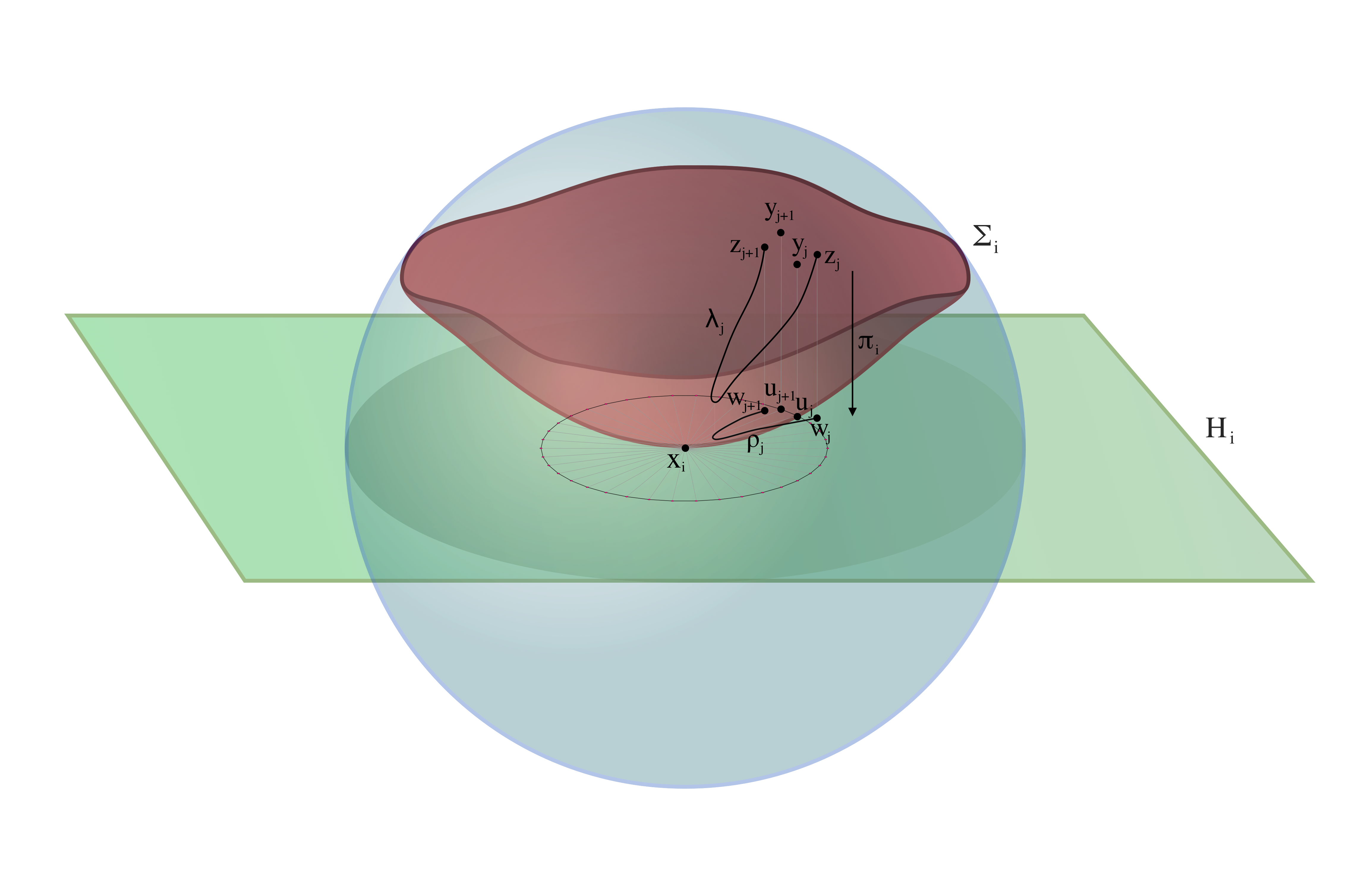
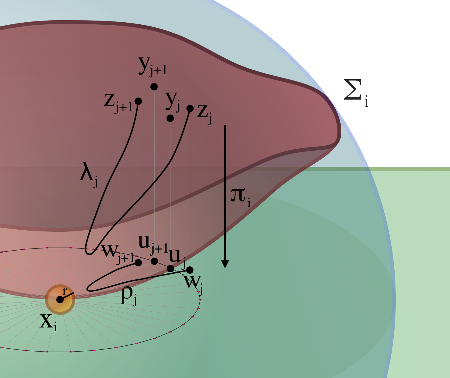
Figure 2. Notation of Subsection 3.3.

Let $y_{j}=\phi_{x_{i}}(u_{j})\in\Sigma_{i}$. By (C-5):

(3.9) $$r<\operatorname{dist}(y_{j},y_{j+1})<r\sqrt{2}.$$

By the definition of $\mathcal{X}$, for any $y_{j}$ there exists an element $z_{j}\in\mathcal{X}$ such that $\operatorname{dist}(z_{j},y_{j})<r$. In particular, by the triangle inequality and (3.9):

(3.10) $$\operatorname{dist}(z_{j},z_{j+1})<(2+\sqrt{2})r,\ \ \operatorname{dist}(x_{i},y_{j})<7r\sqrt{2}<10r.$$

As $\mathcal{G}$ is a collection of good arcs, and $\operatorname{dist}(z_{j},z_{j+1})<4r$, there exists a curve $\lambda_{j}\in\mathcal{G}$ that connects $z_{j}$ and $z_{j+1}$. The length $\lambda_{j}$ is at most $2\operatorname{dist}(z_{j},z_{j+1})<(4+2\sqrt{2})r<7r$.

Denote $w_{j}=\pi_{x_{i}}(z_{j})$ and let $\rho_{j}=\pi_{x_{i}}(\lambda_{j})$.

Lemma 3.11.

We have $z_{j}\in B(x_{i},11r)$. Moreover, $\lambda_{j}\subset B(x_{i},15r)$ and $\rho_{j}$ belongs to $B^{H_{i}}(x_{i},15r)$.

Proof.

From (3.8) we read off that $\operatorname{dist}(x_{i},y_{j})<10r$. As $\operatorname{dist}(y_{j},z_{j})<r$, we conclude that $\operatorname{dist}(x_{i},z_{j})<11r$.

The curve $\lambda_{j}$ has length at most $7r$. No point on $\lambda_{j}$ can be further from $x_{i}$ than $11r+\frac{7}{2}r<15r$. Indeed, if $x$ is outside $B(x_{i},15r)$, then the length of the part of $\lambda_{j}$ from $z_{j}$ to $x$ and the length of the part of $\lambda_{j}$ from $x$ to $z_{j+1}$ are both at least $4r$, contributing to the length of $\lambda_{j}$ being at least $8r$. Therefore, $\lambda_{j}\subset B(x_{i},15r)$.

Now $\pi_{x_{i}}(B(x_{i},15r))\subset B^{H_{i}}(x_{i},15r)$, so $\rho_{j}\subset B^{H_{i}}(x_{i},15r)$. ∎

As $\operatorname{dist}(z_{j},y_{j})<r$, we have $||w_{j}-u_{j}||<r$. By (3.8) and the triangle inequality:

(3.12) $$5r<||w_{j}-x_{i}||<8r.$$

Lemma 3.13.

Let $H_{ij}^{+}$ be the half-plane cut off from $H_{i}$ by the line parallel to the segment joining $u_{j}$ and $u_{j+1}$ and passing through $x_{j}$ such that $u_{j},u_{j+1}\in H_{ij}^{+}$; see Figure 3. The curve $\rho_{j}$ misses $B^{H_{i}}(x_{i},r)$ and $H_{ij}^{+}$. In particular, $\lambda_{j}$ is disjoint from $B(x_{i},r)$.

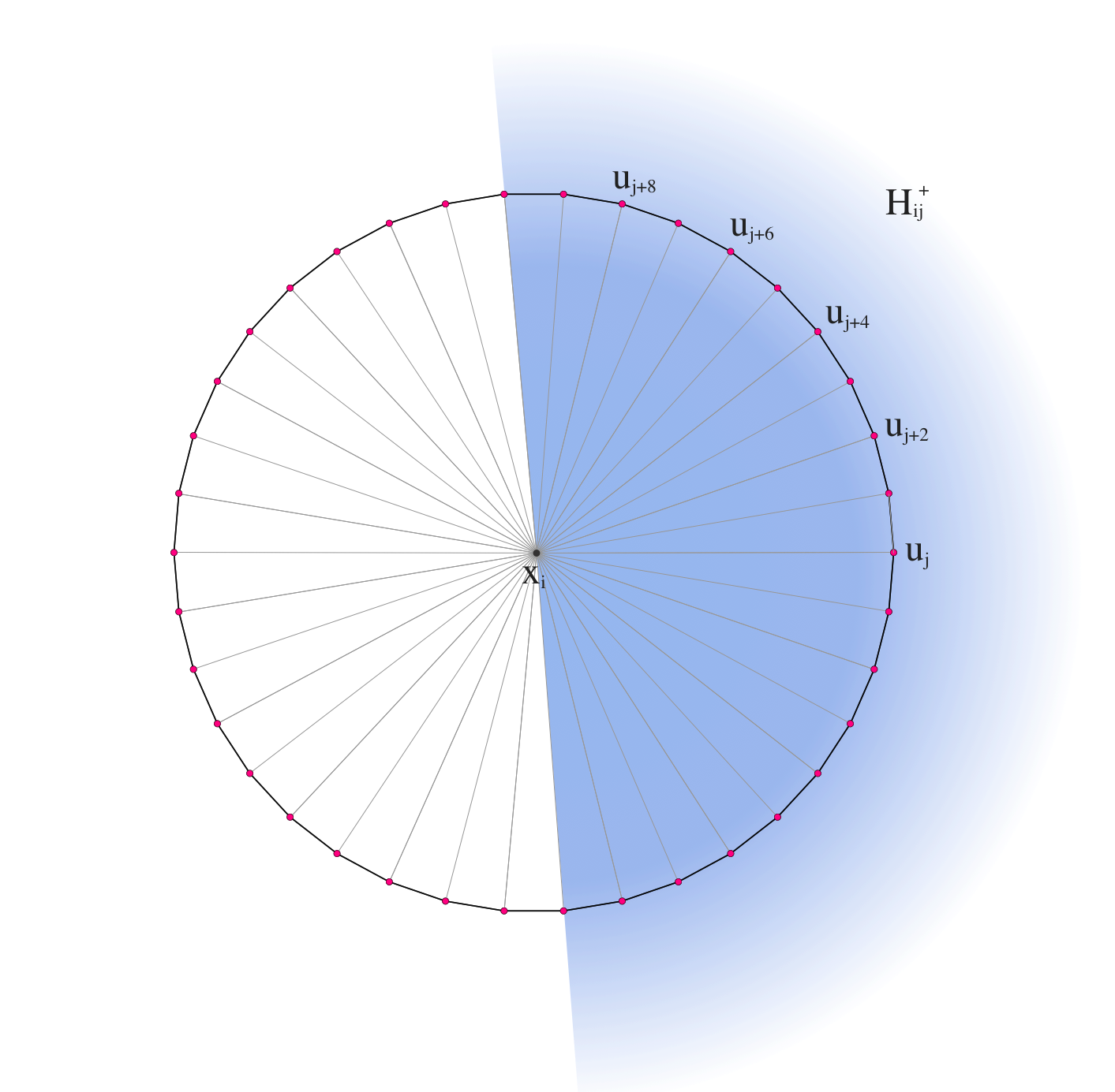
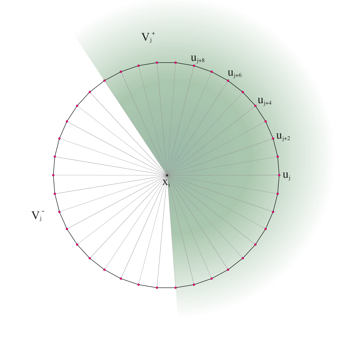
Figure 3. The set $H_{ij}^{+}$ (left) and $V_{j}^{+}$ (right) of the proof of Lemma 3.13 and 3.14.

Proof of Lemma 3.13.

Note that $\pi_{x_{i}}$ being Lipshitz with Lipshitz constant $1$ implies that the length of $\rho_{j}$ is at most $7r$; see (C-5). Suppose towards contradiction that $\rho_{j}$ passes through a point $z\in B(x_{i},r)$. We have $||w_{j}-z||>4r$ and $||w_{j+1}-z||>4r$ by (3.12) and the triangle inequality, hence the length of $\rho_{j}$ is at least $8r$. The contradiction shows that $\rho_{j}$ misses the ball $B^{H_{i}}(x_{i},r)$.

Suppose now $\lambda_{j}$ hits the ball $B(x_{i},r)$, that is, there exists a point $x\in\lambda_{j}\cap B(x_{i},r)$. Then, $\pi_{x_{i}}(x)\in B^{H_{i}}(x_{i},r)$ by (C-5) and so $\rho_{j}$ hits $B^{H_{i}}(x_{i},r)$, contradicting what we have already proved. This shows that $\lambda_{j}$ is disjoint from $B(x_{i},r)$.

To prove that $\rho_{j}$ misses $H_{ij}^{+}$ is analogous. The distance of $u_{j}$ to the boundary of $H_{ij}^{+}$ is equal to $r\sqrt{1/4\sin^{2}(\pi/38)-1/4}$, and it is greater than $6r$. Hence, the distance of $w_{j}$ to $\partial H_{ij}^{+}$ is at least $5r$. That is, if $\rho_{j}$ leaves $H_{ij}^{+}$, then its length must be at least $10r$. Contradiction. ∎

Continuing the proof of Lemma 3.7, we prove the next result.

Lemma 3.14.

For any $j$, the increment of the argument along $\rho_{j}\cup\rho_{j+1}\cup\dots\cup\rho_{j+s}$ with $s=3,4$ is positive.

Proof.

The proof works for larger $s$, we only need the case $3$ and $4$. We prove for $s=3$, leaving the analogous case $s=4$ to the reader. Define: $\overline{\rho}=\rho_{j}\cup\rho_{j+1}\cup\rho_{j+2}$.

Figure 4. Proof of Lemma 3.14. The points $z_{2}$ and $z_{5}$ belong to the disks with centers at $u_{2}$, respectively $u_{5}$. No matter where the points $z_{2}$ and $z_{5}$ are, the oriented angle $\phi$ is positive.

A geometric argument reveals that the oriented angle between the lines $\overline{x_{i}w_{j}}$ and $\overline{x_{i}w_{j+3}}$ is positive; compare Figure 4. Therefore, it is enough to prove that $\overline{\rho}$ does not make a full negative turn while going from $w_{j}$ to $w_{j+3}$.

To this end, let $V^{+}_{j}=H_{ij}^{+}\cup H_{i,j+1}^{+}\cup H_{i,j+2}^{+}\cup H_{i,j+3}^{+}$ and $V^{-}_{j}=H_{i}\setminus V^{+}_{j}$. Then $V^{-}_{j}$ is non-empty $\overline{\rho}$ misses $V^{-}_{j}$. That is, the curve $\overline{\rho}$ does not go around the point $x_{j}$ and the increment of the angle along $\overline{\rho}$ is the same as the oriented angle between the corresponding lines. ∎

Corollary 3.15.

Set $\Delta=\rho_{1}\cup\dots\cup\rho_{38}$. The increment of the argument along $\Delta$ is a positive multiple of $2\pi$.

From this it follows that the winding index of $\Delta$ around $x_{i}$ along is positive.

Remark 3.16.

With a little more care, we could prove that the winding index of $\Delta$ around $x_{i}$ is $1$. We do not need this result.

Corollary 3.17.

The cycle $\Delta$ cuts $H_{i}$ into a finite number of components and $B^{H_{i}}(x_{i},r)$ belongs to a bounded connected component of $H_{i}\setminus\Delta$.

Proof of Corollary 3.17.

The cycle $\Delta$ is closed and has finitely many self-intersections. By Jordan curve theorem, $H_{i}\setminus\Delta$ consists of a finite number of bounded connected components and one unbounded connected component. As the winding index of $\Delta$ around $x_{i}$ is positive, $x_{i}$ cannot possibly belong to the unbounded connected component. By Lemma 3.13, $\Delta$ is disjoint from $B^{H_{i}}(x_{i},r)$. Hence, the whole of $B^{H_{i}}(x_{i},r)$ belongs to the same connected component of $H_{i}\setminus\Delta$. ∎

We denote by $S_{i}\subset\Sigma$ the connected component of $\phi_{x_{i}}(H_{i}\setminus\Delta)$ containing $B(x_{i},r)\cap\Sigma$. To conclude the proof of Lemma 3.7, we choose a point $x\in\Sigma\setminus\Gamma$, where we recall that $\Gamma=\bigcup\gamma_{ij}$. By the definition of $\mathcal{X}$, there exists a point $x_{i}\in\mathcal{X}$ such that $x\in B(x_{i},r)$. The connected component of $\Sigma\setminus\Gamma$ containing $x$ is a subset of $S_{i}$, which is homeomorphic, via $\pi_{x_{i}}$ to an open subset of $H_{i}$. This concludes the proof. ∎

For future use we note the following corollary of the proof of Lemma 3.7.

Corollary 3.18.

Any connected component of $\Sigma\setminus\Gamma$ belongs to $B(x_{i},22r)$ for some $x_{i}\in\mathcal{X}$.

Proof.

With the notation of the proof of Lemma 3.7, we let $S$ be a connected component of $\Sigma\setminus\Gamma$. Take $x\in S$ and let $x_{i}\in\mathcal{X}$ be such that $\operatorname{dist}(x_{i},x)<r$. Then $x\in\phi_{x_{i}}(S_{i})$ and then, as $\phi_{x_{i}}(S_{i})$ is a connected component of $\Sigma\setminus(\lambda_{1}\cup\dots\cup\lambda_{38})\subset\Sigma\setminus\Gamma$, we clearly have $S\subset\phi_{x_{i}}(S_{i})$. Now $S_{i}\subset B^{H_{i}}(x_{i},15r)$, so $\phi_{x_{i}}(S_{i})\subset B(x_{i},15\sqrt{2}r)\subset B(x_{i},22r)$. Hence, $S\subset B(x_{i},22r)$ as desired. ∎

3.4. The property (G-2)

We will now show that under the same conditions as in Lemma 3.7 we can improve the collection $\mathcal{G}$ in such a way that (G-2) is satisfied.

Lemma 3.19.

Suppose $\mathcal{G}$ is a collection of good arcs. If $29r<R_{0}$, then there exists a collection of good arcs $\widetilde{\gamma}_{ij}$ satisfying (G-2).

Proof.

Choose $\varepsilon>0$ such that for any $i,j$ we have $\ell(\gamma_{ij})+\varepsilon<2||x_{i}-x_{j}||$. We introduce the following notion.

Definition 3.20.

A boundary bigon is a pair of two arcs $\alpha$ and $\beta$ with common end points and disjoint interiors such that $\alpha$ and $\beta$ are parts of some curves $\gamma_{ij}$ and $\gamma_{kl}$.

A bigon $(D,\alpha,\beta)$ is a triple $(D,\alpha,\beta)$, where $(\alpha,\beta)$ form a boundary bigon and $D$ is an embedded disk $D\hookrightarrow\Sigma$ such that $\partial D=\alpha\cup\beta$ and $D$ belongs to $B(x_{i},17r)$ for some $x_{i}$, which is an end point of a curve in $\mathcal{G}$ whose part is either $\alpha$ or $\beta$.

Suppose $\gamma_{ij}$ and $\gamma_{kl}$ are distinct arcs. Let $s$ be the number of their intersection points. Then, $\gamma_{ij}$ and $\gamma_{kl}$ form $s-1$ boundary bigons. The proof of Lemma 3.19 relies on successively removing boundary bigons.

Lemma 3.21.

Every boundary bigon is a bigon.

Proof.

We know that $\ell(\gamma_{ij}),\ell(\gamma_{kl})<8r$, because $\operatorname{dist}(x_{i},x_{j})<4r$ and $\operatorname{dist}(x_{k},x_{l})<4r$. From this it follows that $\gamma_{ij}\subset B(x_{i},6r)$ and $\gamma_{kl}\subset B(x_{k},6r)$. Indeed, if $x\in\gamma_{ij}$ is outside $B(x_{i},6r)$, then, by triangle inequality $x\notin B(x_{j},2r)$. Therefore, $\ell(\gamma_{ij})\geq\operatorname{dist}(x_{i},x)+\operatorname{dist}(x,x_{j})>8r$.

As $\gamma_{kl}\cap\gamma_{ij}$ is not empty, we conclude that $\gamma_{kl}\cup\gamma_{ij}\subset B(x_{i},12r)$. Since $12\sqrt{2}r<17r<R_{0}$, the map $\pi_{x_{i}}\colon B(x_{i},17r)\to H_{i}$ is well-defined and its image $U_{i}$ contains the ball $B^{H_{i}}(x_{i},12r)$; see (C-2), (C-3). Let $\widehat{\alpha},\widehat{\beta}=\pi_{x_{i}}(\alpha),\pi_{x_{i}}(\beta)$. Then $\widehat{\alpha}\cup\widehat{\beta}$ is a simple closed curve on $H_{i}$ contained in $B^{H_{i}}(x_{i},12r)$. By Jordan curve theorem, there exists a disk $\widehat{D}$ in $B^{H_{i}}(x_{i},12r)$ such that $\partial\widehat{D}=\widehat{\alpha}\cup\widehat{\beta}$. The desired disk $D$ is obtained as $\phi_{x_{i}}(\widehat{D})$. By (C-5), $D\subset B(x_{i},12\sqrt{2}r)\subset B(x_{i},17r)$. ∎

Corollary 3.22.

Let $(\alpha,\beta)$ be a boundary bigon. If $D_{1}$, $D_{2}$ are two embeddings of a disk such that $(D_{1},\alpha,\beta)$ and $(D_{2},\alpha,\beta)$ are bigons, then the images of $D_{1}$ and $D_{2}$ coincide.

Proof.

Suppose that $D_{1}$ and $D_{2}$ do not coincide. Their interiors are disjoint, for otherwise $\Sigma$ has self-intersections. Assume that $D_{1}\in B(x_{i},17r)$ and $D_{2}\in B(x_{i^{\prime}},17r)$, where $i^{\prime}$ is any of the $i,j,k,\ell$ (we keep the notation of Lemma 3.21). Note that $\operatorname{dist}(x_{i},x_{j})<4r$ and $\operatorname{dist}(x_{i},x_{k}),\operatorname{dist}(x_{i},x_{\ell})<12r$. Therefore, in the worst case scenario, when $D_{2}\subset B(x_{k},17r)$ or $D_{2}\subset B(x_{\ell},17r)$, we still have that $D_{2}\subset B(x_{i},29r)$. Then $D_{1}\cup D_{2}$ glue to a sphere in $B(x_{i},29r)$. But $29r<R_{0}$ and so $D_{1}\cup D_{2}$ belongs to a graph patch. This is impossible. ∎

Continuing the proof of Lemma 3.19, we introduce more terminology. Let $D=(D,\alpha,\beta)$ be a bigon. We say that

• $D$ is minimal if $D$ does not contain any smaller bigon;

• $D$ is desolate if $D$ does not contain any point $x_{i}$;

• $D$ is inhabitated if $D$ contains at least one of $x_{i}$; see Figure 5.

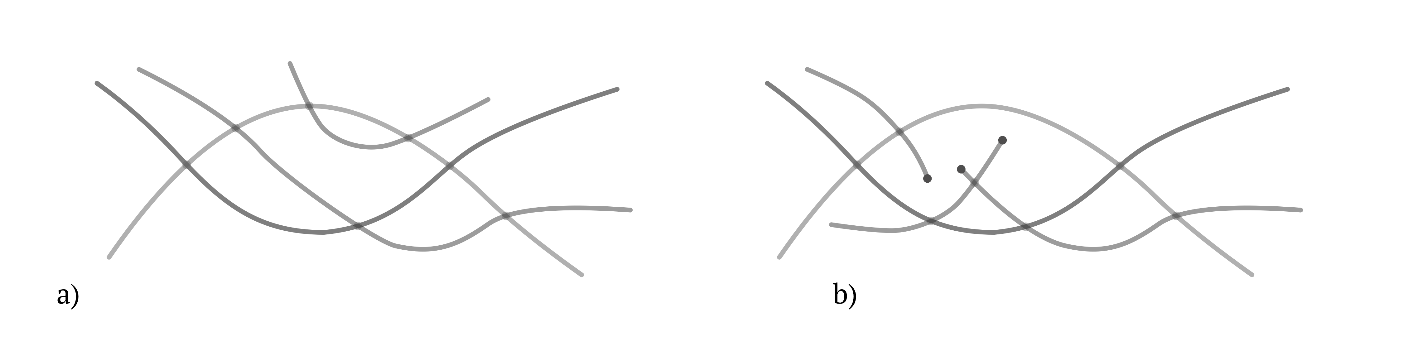
Figure 5. A desolate and an inhabitated bigon.

We will now describe a procedure called bigon removal; see Figure 6. Suppose $(D,\alpha,\beta)$ is a bigon. We can swap the roles of $\alpha$ and $\beta$, if needed, to ensure that $\alpha$ is not longer than $\beta$. The curve $\beta$ is replaced by a curve $\beta^{\prime}$ parallel to the curve $\alpha$. It is clear that the change can be made in such a way that the length of $\beta$ is not increased by more than $\varepsilon/2$. It might happen that one of the vertices $\alpha\cap\beta$ of the bigon is actually a starting point of the two curves in $\mathcal{G}$, whose parts form a bigon. The picture in Figure 6 should be slightly altered, but the argumentation is the same.

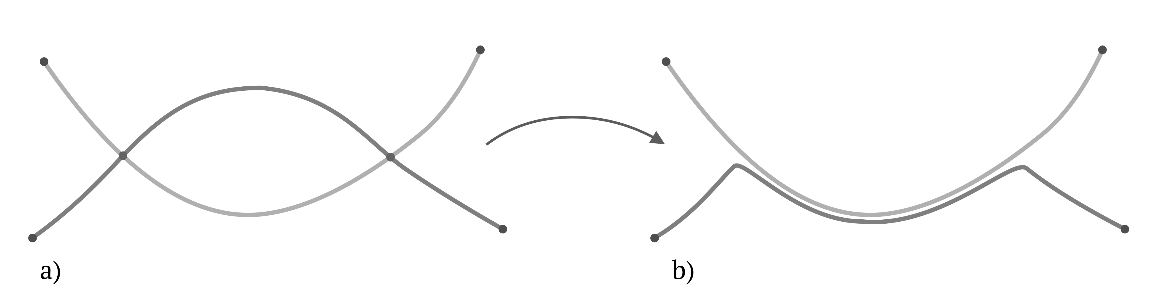
Figure 6. Bigon removal: (a) output bigon, (b) fragment of one curve replaced with the approximation of the second.

Lemma 3.23.

If $D$ is a desolate minimal bigon, bigon removal procedure applied to $D$ decreases the number of desolate bigons by $1$ and creates no other bigons.

Proof.

By Corollary 3.22, the number of bigons between two different curves $\gamma,\gamma^{\prime}\in\mathcal{G}$ is equal to $|\gamma\cap\gamma^{\prime}|-1$. Therefore, we will strive to show that the number of intersection points between all curves in $\mathcal{G}$ decreases after bigon removal.

Let $\gamma_{kl}$ and $\gamma_{st}$ be such that $\alpha\subset\gamma_{kl}$ and $\beta\subset\gamma_{st}$. The $\gamma^{\prime}_{st}$ be the curve $\gamma_{st}$ with $\beta$ replaced by $\beta^{\prime}$. We have

$$|\gamma_{kl}\cap\gamma_{st}^{\prime}|=|\gamma_{kl}\cap\gamma_{st}|-2.$$

Suppose $\gamma_{uw}$ is another curve in $\mathcal{G}$. If it does not hit the bigon $D$, we have that $\gamma_{st}\cap\gamma_{uw}=\gamma_{st}^{\prime}\cap\gamma_{uw}$, so the number of intersection points is preserved. If $\gamma_{uw}$ hits the bigon $D$, we look at connected components of $\gamma_{uw}\cap D$. Each such connected component $\delta$ is an arc, and if $|\delta\cap\alpha|=2$ or $|\delta\cap\beta|=2$, the arc $\delta$ and the relevant part of $\alpha$ or $\beta$ form a bigon contained in $D$, contradicting minimality of $D$. If $|\delta\cap(\alpha\cup\beta)|=1$, one of the end points of $\delta$ is inside $D$, but such an end point must be an end point of $\gamma_{st}$, that is, it must be a point from $\mathcal{X}$. This contradicts the condition that $D$ be desolate.

The only remaining possibility is that $|\delta\cap\alpha|=|\delta\cap\beta|=1$. This, in turn, shows that $|\gamma_{uw}\cap\alpha|=|\gamma_{uw}\cap\beta|$. Now, by construction $|\gamma_{uw}\cap\beta^{\prime}|=|\gamma_{uw}\cap\alpha|$. Eventually $|\gamma_{uw}\cap\beta|=|\gamma_{uw}\cap\beta^{\prime}|$, that is, $|\gamma_{uw}\cap\gamma_{st}^{\prime}|=|\gamma_{uw}\cap\gamma_{st}|$. In other words, no new bigons are created. ∎

Remark 3.24.

The statement of Lemma 3.23 need not hold if $D$ is inhabitated. A bigon removal procedure can create new bigons, both inhabitated and desolate, whose number is rather hard to control; see Figure 7.

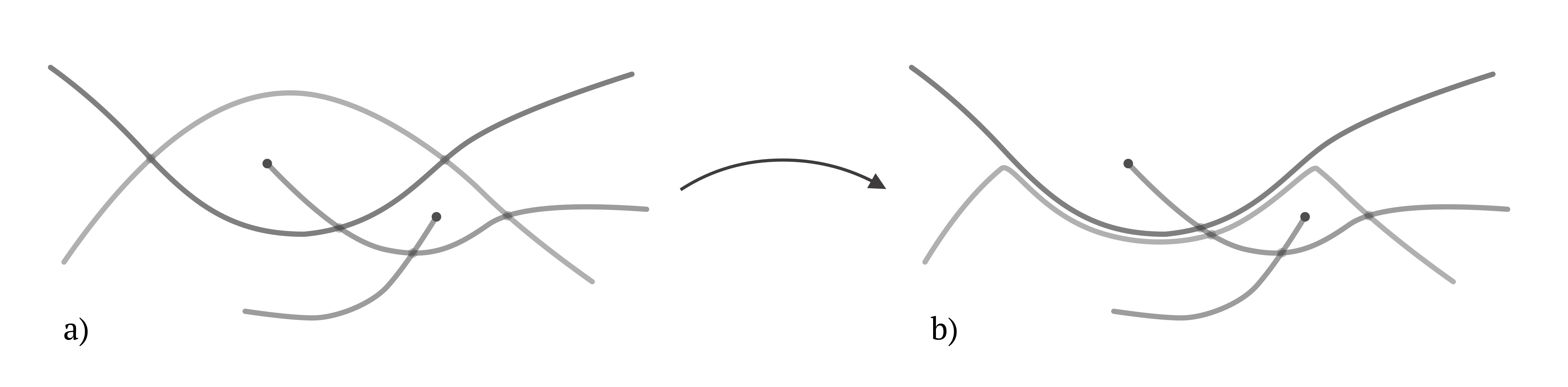
Figure 7. An attempt to remove an inhabitated bigon results in creating another inhabitated bigon. There is a little control on the number of bigons that can be produced in this way.

After a single bigon removal procedure, the length of one of the curves $\gamma_{ij}$ can increase, we decrease $\varepsilon$ so that $\ell(\gamma_{ij})+\varepsilon<2\operatorname{dist}(x_{i},x_{j})$ for all $(i,j)\in\mathcal{I}$.

We now apply inductively the bigon removal procedure to all minimal desolate bigons, until there are no minimal desolate bigons. This requires a finite number of steps. We make the following trivial observation.

Lemma 3.25.

If there are no minimal desolate bigons, there are no desolate bigons at all.

From now on we will assume that the set $\mathcal{G}$ of curves is such that there are no desolate bigons. The following lemma concludes the proof of Lemma 3.19.

Lemma 3.26.

Suppose curves $\gamma_{ij}$ and $\gamma_{kl}$ do not form desolate bigons. Then, the number of intersection points between $\gamma_{ij}$ and $\gamma_{kl}$ is bounded by $\mathcal{T}(17)$.

Proof.

Suppose $\gamma_{ij}$ and $\gamma_{kl}$ are not disjoint. By Lemma 3.21, each bigon formed by $\gamma_{ij}$ and $\gamma_{kl}$ belongs to $B(x_{i},17r)$. All such bigons have pairwise disjoint interiors. Moreover, each bigon is inhabitated. The number of bigons is bounded from above by the total number of points of $\mathcal{X}$ in $B(x_{i},17r)$, which is $\mathcal{T}(17)$ according to Proposition 3.4.

The number of intersection points is not greater than the number of bigons. The lemma follows. ∎

The proof of Lemma 3.19 is complete. ∎

4. Triangulation

4.1. Bounding number of triangles

Proposition 4.1.

Let $\mathcal{X}$ be an $r$-net with $29r<R_{0}$. Suppose $\mathcal{G}$ is a good tame collection of arcs. Then $\Sigma$ can be triangulated with at most $S(\Sigma)$ triangles with

(4.2) $$S(\Sigma)=\frac{1}{12}\mathcal{T}(4)^{2}\mathcal{T}(8)^{2}\mathcal{T}(12)^{2}\mathcal{T}(15)^{2}\mathcal{T}(17)^{2}|\mathcal{X}|.$$

Proof.

The proof of Proposition 4.1 takes the rest of Subsection 4.1. The triangulation is constructed by subdivision of $\Gamma=\bigcup\gamma_{ij}$. The vertices are going to be the points in $\mathcal{X}$ as well as the intersection points $\gamma_{ij}\cap\gamma_{kl}$. We first bound the total number of intersection points of $\gamma_{ij}$.

Lemma 4.3.

Suppose $x_{i}\in\mathcal{X}$. The total number of points triples $j,k,l$ such that $\gamma_{ij}\cap\gamma_{kl}\neq\emptyset$ is less than or equal to $2\mathcal{T}(4)\mathcal{T}(8)\mathcal{T}(12)$.

Proof.

First of all, number of indices $j$ such that $\operatorname{dist}(x_{i},x_{j})<4r$ is at most $\mathcal{T}(4)$. Next, a point $x\in\gamma_{ij}\cap\gamma_{kl}$ has to lie at distance less than $4r$ from either $x_{i}$ or $x_{j}$. Suppose $\operatorname{dist}(x_{i},x)<4r$. The same argument shows that either $\operatorname{dist}(x_{k},x)<4r$ or $\operatorname{dist}(x_{l},x)<4r$. Switch $k$ and $l$ so that $\operatorname{dist}(x_{k},x)<4r$. Then $\operatorname{dist}(x_{i},x_{k})<8r$ and $\operatorname{dist}(x_{i},x_{l})<8r+\operatorname{dist}(x_{k},x_{l})<12r$.

The total number of choices of $x_{j}$ is $\mathcal{T}(4)$. The total number of choices of $x_{k}$ and $x_{l}$ is $2\mathcal{T}(8)\mathcal{T}(12)$: the factor $2$ comes from chosing whether $\operatorname{dist}(x_{i},x)<4r$ or $\operatorname{dist}(x_{j},x)<4r$. ∎

Let now

$$\mathcal{Z}=\bigcup_{(l,k)\neq(i,j)\neq(k,l)}\{\gamma_{ij}\cap\gamma_{kl}\}.$$

Note that $\mathcal{X}\subset\mathcal{Z}$. Indeed, it is not hard to see that for any $i$ there are at least two points $j,l$ such that $(i,j),(i,l)\in\mathcal{I}$ and then $x_{i}\in\gamma_{ij}\cap\gamma_{il}$.

Lemma 4.4.

We have $|\mathcal{Z}|<\frac{1}{2}\mathcal{T}(4)\mathcal{T}(8)\mathcal{T}(12)\mathcal{T}(17)|\mathcal{X}|$.

Proof.

Take $x_{i}\in\mathcal{X}$. By Lemma 4.3 there are at most $2\mathcal{T}(4)\mathcal{T}(8)\mathcal{T}(12)$ configurations $j,k,l$ such that $\gamma_{ij}\cap\gamma_{kl}\neq\emptyset$. Therefore, the total number of quadruples $i,j,k,l$ such that $\gamma_{ij}\cap\gamma_{kl}\neq\emptyset$ is $\frac{1}{2}\mathcal{T}(4)\mathcal{T}(8)\mathcal{T}(12)|\mathcal{X}|$. The difference of factors $2$ and $1/2$ corresponds to the following observation: when summing over the indices $i$, each quadruple $i,j,k,l$ is actually counted four times. First, we can switch $i$ with $j$. Then we can switch the pairs $(i,j)$ and $(k,l)$.

If two curves $\gamma_{ij}$ and $\gamma_{kl}$ intersect, by (G-2) the total number of intersections is at most $\mathcal{T}(17)$. The lemma follows. ∎

The same argument yields

Lemma 4.5.

Let $\sigma>0$ be such that $(\sigma+1/4)r<R_{0}$. Let $\mathcal{Z}^{\sigma}_{i}$ be the number of points $z\in\mathcal{Z}$ such that $z\in B(x_{i},\sigma r)$. Then $|\mathcal{Z}^{\sigma}_{i}|<\frac{1}{2}\mathcal{T}(4)\mathcal{T}(8)\mathcal{T}(12)\mathcal{T}(17)\mathcal{T}(\sigma)$.

Proof.

We use the proof of Lemma 4.4. On passing from the number of triples $j,k,l$ such that $\gamma_{ij}\cap\gamma_{kl}\neq\emptyset$ we multiply by the bound of the number of points in $B(x_{i},\sigma r)$, that is, $\mathcal{T}(\sigma)$, instead of the total number of points $x_{i}$, that is, $|\mathcal{X}|$. ∎

Now we pass to construction of triangulation. By the property (G-1), each connected component of $\Sigma\setminus\Gamma$ is a subset of $\mathbb{R}^{2}$. Take such a connected component $C$. Its boundary is a union of (parts of) curves $\gamma_{ij}$ intersecting at points of $\mathcal{Z}$. We think of $C$ as a polygon with vertices $\mathcal{Z}$, though we do not necessarily assume that $C$ has connected boundary. We triangulate this polygon by adding curves that connect vertices of $\mathcal{Z}$. This provides us with a triangulation. In particular, the triangulation has the following property.

Property 4.6.

An edge of the triangulation connects two elements in $\mathcal{Z}$, which belong to the closure of the same connected component of $\Sigma\setminus\Gamma$.

To estimate the number of triangles we use the following lemma.

Lemma 4.7.

Suppose $z_{1},z_{2}\in\mathcal{Z}$ and $z_{1},z_{2}$ belong to the closure of the same connected component $S_{z}$ of $\Sigma\setminus\Gamma$. Then, there exists $x_{i}\in\mathcal{X}$ such that $z_{1},z_{2}\in\Sigma\cap B(x_{i},15r)$.

Proof.

Let $x_{i}$ be a point on $\Sigma$ such that $\operatorname{dist}(x_{i},z_{1})<r$. Set $y_{1}=\pi_{x_{i}}(z_{1})$, $y_{2}=\pi_{x_{i}}(z_{2})$. Consider the cycle $\Delta$ on $H_{i}$ as in Corollary 3.15. By Corollary 3.15 there is a piecewise smooth simple closed curve $\Delta_{0}\subset\Delta$ such that $\Delta_{0}$ cuts $H_{i}$ into two components: the component $S_{i}$, which is bounded and contains $B^{H_{i}}(x_{i},r)$ and the other, which is unbounded. As $y_{1}\in B^{H_{i}}(x_{i},r)$, the closure of $\pi_{x_{i}}(S_{z})$ must belong to $S_{i}$. In particular, $y_{2}$ cannot belong to $H_{i}\setminus\overline{S_{i}}$. Now, $\phi_{x_{i}}(\Delta)=\pi_{x_{i}}^{-1}(\Delta)$ is a subset of the union of the curves $\lambda_{j}$, all belonging to $B(x_{i},15r)$. Therefore, $z_{2}\in B(x_{i},15r)$ as well.

∎

Corollary 4.8.

The total number of edges in the triangulation is bounded from above by

$$\frac{1}{8}\mathcal{T}(4)^{2}\mathcal{T}(8)^{2}\mathcal{T}(12)^{2}\mathcal{T}(15)^{2}\mathcal{T}(17)^{2}|\mathcal{X}|.$$

Proof.

By Lemma 4.7 and Property 4.6, any two edges connecting points $z_{1}$ and $z_{2}$ belong to the same $B(x_{i},15r)\cap\Sigma$ for some $x_{i}\in\mathcal{Z}$. The number of pairs $z_{1},z_{2}$ of points $\mathcal{Z}$ in $B(x_{i},15r)$ is equal to

$$\frac{1}{2}|\mathcal{Z}^{15}_{i}|^{2}\leq\frac{1}{8}\mathcal{T}(4)^{2}\mathcal{T}(8)^{2}\mathcal{T}(12)^{2}\mathcal{T}(15)^{2}\mathcal{T}(17)^{2}.$$

Summing up over all $x_{i}\in\mathcal{X}$ we get the result. ∎

The rest of the proof of Proposition 4.1 is straightforward. Each edge belongs to precisely two triangles and each triangle has three edges. ∎

4.2. Proof of Theorem 1.1

Suppose $\mathcal{E}^{\ell}_{p}(\Sigma)=E$ and let $C_{0}=2^{-1/2}\min(c_{1},c_{2}^{-1/p\alpha})$; compare Corollary 2.5. Here, $\alpha=1-2\ell/p$. Set $r=\frac{1}{29}C_{0}E^{-1/p\alpha}$. Choose a net of points $\mathcal{X}$ with this given $r$. By Proposition 3.3, we have

(4.9) $$|\mathcal{X}|<C_{1}AE^{2/p\alpha},$$

where $C_{1}=2^{n/2+8}29^{2}V_{2}C_{0}^{-2}$.

Let $\mathcal{G}$ be a collection of good arcs connecting some of the pairs of points of $\mathcal{X}$; such collection exists by Proposition 3.6, because $4r<29r<R_{0}=C_{0}E^{-1/p\alpha}$. The collection $\mathcal{G}$ can be improved to a tame collection of good arcs by Lemmata 3.7 and 3.19, which work because $29r<R_{0}$. A tame collection of arcs provides a triangulation with the number of triangles bounded above by $S(\Sigma)$ triangles; see Proposition 4.1. In total, the number of triangles is bounded above by $C_{2}AE^{2/p\alpha}$, where

$$C_{2}=\frac{1}{12}\mathcal{T}(4)^{2}\mathcal{T}(8)^{2}\mathcal{T}(12)^{2}\mathcal{T}(15)^{2}\mathcal{T}(17)^{2}C_{1}.$$

By construction, each triangle is an image of a subset of a plane $H_{i}$ (for some $i$) under the map $\phi_{x_{i}}$, which has bounded derivative and bounded distortion by Corollary 2.5 and Corollary 2.7.

References

- [1] I. Fáry. Sur la courbure totale d’une courbe gauche faisant un nœud. Bull. Soc. Math. France, 77:128–138, 1949.
- [2] J. Hass. The geometry of the slice-ribbon problem. Math. Proc. Cambridge Philos. Soc., 94(1):101–108, 1983.
- [3] M. Jungerman and G. Ringel. Minimal triangulations on orientable surfaces. Acta Math., 145(1-2):121–154, 1980.
- [4] S. Kolasiński. Geometric Sobolev-like embedding using high-dimensional Menger-like curvature. Trans. Amer. Math. Soc., 367(2):775–811, 2015.
- [5] S. Kolasiński, P. Strzelecki, and H. von der Mosel. Compactness and isotopy finiteness for submanifolds with uniformly bounded geometric curvature energies. Comm. Anal. Geom., 26(6):1251–1316, 2018.
- [6] J. Milnor. On the total curvature of knots. Ann. of Math. (2), 52:248–257, 1950.
- [7] P. Strzelecki, M. Szumańska, and H. von der Mosel. On some knot energies involving Menger curvature. Topology Appl., 160(13):1507–1529, 2013.
- [8] P. Strzelecki and H. von der Mosel. Integral Menger curvature for surfaces. Adv. Math., 226(3):2233–2304, 2011.