Delay-Compensated Distributed PDE Control of Traffic with Connected/Automated Vehicles

Abstract

We develop an input delay-compensating design for stabilization of an Aw-Rascle-Zhang (ARZ) traffic model in congested regime which is governed by a $2\times 2$ first-order hyperbolic nonlinear PDE. The traffic flow consists of both adaptive cruise control-equipped (ACC-equipped) and manually-driven vehicles. The control input is the time gap of ACC-equipped and connected vehicles, which is subject to delays resulting from communication lag. For the linearized system, a novel three-branch bakcstepping transformation with explicit kernel functions is introduced to compensate the input delay. The transformation is proved to be bounded, continuous and invertible, with explicit inverse transformation derived. Based on the transformation, we obtain the explicit predictor-feedback controller. We prove exponential stability of the closed-loop system with the delay compensator in $L_{2}$ norm. The performance improvement of the closed-loop system under the proposed controller is illustrated in simulation.

I Introduction

Traffic congestion has become a severe worldwide social issue. Stop-and-go traffic is a common phenomenon in congested highway traffic[30], which results from a small perturbation, such as a delay in a driver’s response, propagating backward in traffic flow[8, 20]. The stop-and-go oscillation in traffic flow leads to poorer driving experience, higher fuel consumption and a high accident risk. One promising way to reduce the oscillation in the congested regime is to develop control design tools that exploit the capabilities of automated and connected vehicles, such as manipulation of the time gap setting of ACC-equipped and connected vehicles [12, 4].

PDE-based models have established a realistic description of the traffic dynamics [10, 11, 3, 17, 29] by capturing the temporal and spatial dynamics of the traffic density and the traffic speed along the considered highway stretch. Boundary control [16, 34, 35, 37, 38, 33], and in-domain manipulation [9], [31] are both developed to stabilize the traffic flow. Traffic state estimations are also considered in different situations [35], [5], [13]. Due to the information transmission or (and) reaction time of drivers [7], there are usually time delays in the traffic flow control process, see, e.g., [15] for delays in feedback. Therefore, it is necessary to study the traffic flow control involving delays. However, few papers on traffic control consider delay compensation.

We consider an Aw-Rascle-Zhang (ARZ) traffic model in congested regime comprising manually-driven vehicles and ACC vehicles, which are subject to input delays. The model is composed of $2\times 2$ first-order hyperbolic PDEs whose states are traffic density and traffic speed. In order to eliminate the stop-and-go waves, a distributed actuation using the time-gap of the ACC vehicles is employed for control. If the actuator delay is present and sufficiently large, the state feedback control proposed in [4] may become destabilizing.

Relevant advances have been achieved towards the controlling of diffusion-driven distributed parameter systems with delays. Early predictor-based boundary controller is developed using the PDE backstepping method in [18], which stabilizes an unstable reaction-diffusion PDE with arbitrarily long input delay. The aforementioned method has been extended to a 3-D formation control problem to compensate for the effect of potential input delays [25]. For state delays in an unstable reaction-diffusion PDE, a boundary feedback has been developed using backstepping in [14]. Recently, a delay-compensator was designed for an unstable reaction-diffusion PDE via distributed actuation in [24]. Alternatively, series control design approaches based on Lyapunov-Krasovskii functions have been proposed in [27] and [28], respectively. A boundary feedback to compensate a constant input delay for an unstable reaction-diffusion PDE has been developed in [22], using spectral reduced-order models which approximate the infinite-dimensional system by a finite-dimensional one. A similar method is used for in-domain stabilization of reaction-diffusion PDEs with time-and spatially-varying delays in [19].

Most studies on delay-compensator design are for parabolic PDEs. There are fewer results on hyperbolic PDEs with delays. An example of first-order hyperbolic PDE is given in [26], where a backstepping boundary control is designed for compensating the input delay. State delay and measurement delay is addressed in [23]. In the context of robustness analysis, a delay-robust boundary feedback has been proposed for a $2\times 2$ linear hyperbolic PDEs in [2]. Both in [6] and [32], the authors introduce an equivalent delay system representation to first-order hyperbolic PDEs, which transforms the coupled PDE-ODE systems to ODE systems with input delays.

The overall challenge addressed in this work is the design of an in-domain delay-compensator for a $2\times 2$ hyperbolic PDE by employing the PDE backstepping method while dealing with a dynamic boundary condition which results in a $2\times 2$ hyperbolic PDE-ODE cascade system. The usual Volterra integral transformation cannot be applied directly to control design because the resulting kernel equation is unsolvable. Therefore, we propose a three-branch affine Volterra transformation which contains the state of the ODE, namely, the traffic speed at the outlet boundary. The transformation with explicit kernel functions has a different form in each of the three intervals. Although there are three intervals, the transformation is proved to be continuous in its domain. Further, we derive the explicit inverse transformation which is bounded and continuous too. Based on the transformation, we obtain an explicit delay-compensator, composed of the feedback of the states and the historical actuator state. The compensator stabilizes the traffic flow with input delay via manipulation of the time gap of the ACC-equipped vehicles in-domain. We prove the closed-loop system is $L_{2}$ exponentially stable, by establishing the $L_{2}$ stability of the target system and the norm equivalence between the target system and the original system based on the fact that the transformation is invertible.

The structure of the paper is as follows. In Section II, we introduce the model. In Section III, we design the delay-compensator using the backstepping method. Section IV presents the proof of the $L_{2}$ norm exponential stability of the close-loop system. The effectiveness of the proposed delay-compensated controller is illustrated with numerical simulations in Section V. The conclusion is given in Section VI.

Notation: Throughout the paper, we adopt the following notation to define $L_{2}$-norm for $f(\cdot)\in L_{2}(0,L)$, $g(\cdot,\cdot)\in L_{2}((0,L)\times(0,D))$ :

$$\rVert f\rVert^{2}_{L_{2}}=\int_{0}^{L}|f(x)|^{2}\mathrm{d}x,~{}~{}\rVert g\rVert^{2}_{L_{2}}=\int_{0}^{L}\int_{0}^{D}|g(x,s)|^{2}\mathrm{d}s\mathrm{d}x.$$

II Model Description

II-A ARZ Traffic model with mixed vehicles

We consider the ARZ traffic model of highway introduced in [4] but an input delay which acts on adaptive cruise control-equipped (ACC-equipped) vehicles is addressed. The state variables of the model are the traffic density $\breve{\rho}(x,t)$ and the traffic speed $\breve{v}(x,t),$ both defined in domain $(x,t)\in[0,L]\times\mathbb{R}^{+}$ where $t$ is time, $x$ is the spatial variable denoting the position on the concerned highway. Constant $L>0$ denotes the length of the concerned highway stretch. Define $\breve{v}(x,t)\in(0,v_{\rm{f}}]$ with $v_{\rm{f}}$ being free-flow speed. We consider a mixed traffic, consisting of both manual and ACC-equipped vehicles with the percentage of ACC-equipped vehicles with respect to total vehicles being $\alpha$. Let $\breve{h}_{\mathrm{acc}}(x,t)$ denote the time-gap of the ACC-equipped vehicle at $x$ from its leading vehicle, which is the control input because a vehicle with ACC can automatically adjust its speed to maintain a desired distance (or, say, a time-gap) from vehicles ahead. Due to the lag of information transmission from the control center to each individual ACC vehicle, there often exists input delay. Expressed with equations, the traffic flow control system we consider is:

$$\breve{\rho}_{t}(x,t)= -\breve{\rho}_{x}(x,t)\breve{v}(x,t)-\breve{\rho}(x,t)\breve{v}_{x}(x,t),$$ (1)

$$\breve{v}_{t}(x,t)= -\breve{\rho}(x,t)\frac{\partial V_{\rm{mix}}(\breve{\rho}(x,t),\breve{h}_{\rm{acc}}(x,t-D))}{\partial\breve{\rho}}\breve{v}_{x}(x,t)$$

$$-\breve{v}(x,t)\breve{v}_{x}(x,t)$$

$$+\frac{V_{\rm{mix}}(\breve{\rho}(x,t),\breve{h}_{\rm{acc}}(x,t-D))-\breve{v}(x,t)}{\tau_{\rm{mix}}(\alpha)},$$ (2)

$$\breve{\rho}(0,t)= q_{\rm{in}}/\breve{v}(0,t),$$ (3)

$$\breve{v}_{t}(L,t)= \frac{V_{\rm{mix}}(\breve{\rho}(L,t),\breve{h}_{\rm{acc}}(L,t-D))-\breve{v}(L,t)}{\tau_{\rm{mix}}(\alpha)},$$ (4)

where $D$ is the delay on the domain-wide actuated time gap input, and

$$\tau_{\rm{mix}}(\alpha)= \frac{1}{\frac{\alpha}{\tau_{\rm{acc}}}+\frac{1-\alpha}{\tau_{\rm{m}}}},~{}0\leq\alpha\leq 1$$ (5)

is time constant for a mixture traffic which depends on both time constant $\tau_{\rm{acc}}$ of ACC vehicles and time constant $\tau_{\rm{m}}$ of manual vehicles.

Fig. 1: $\tau_{\rm mix}$ varies with $\alpha$.

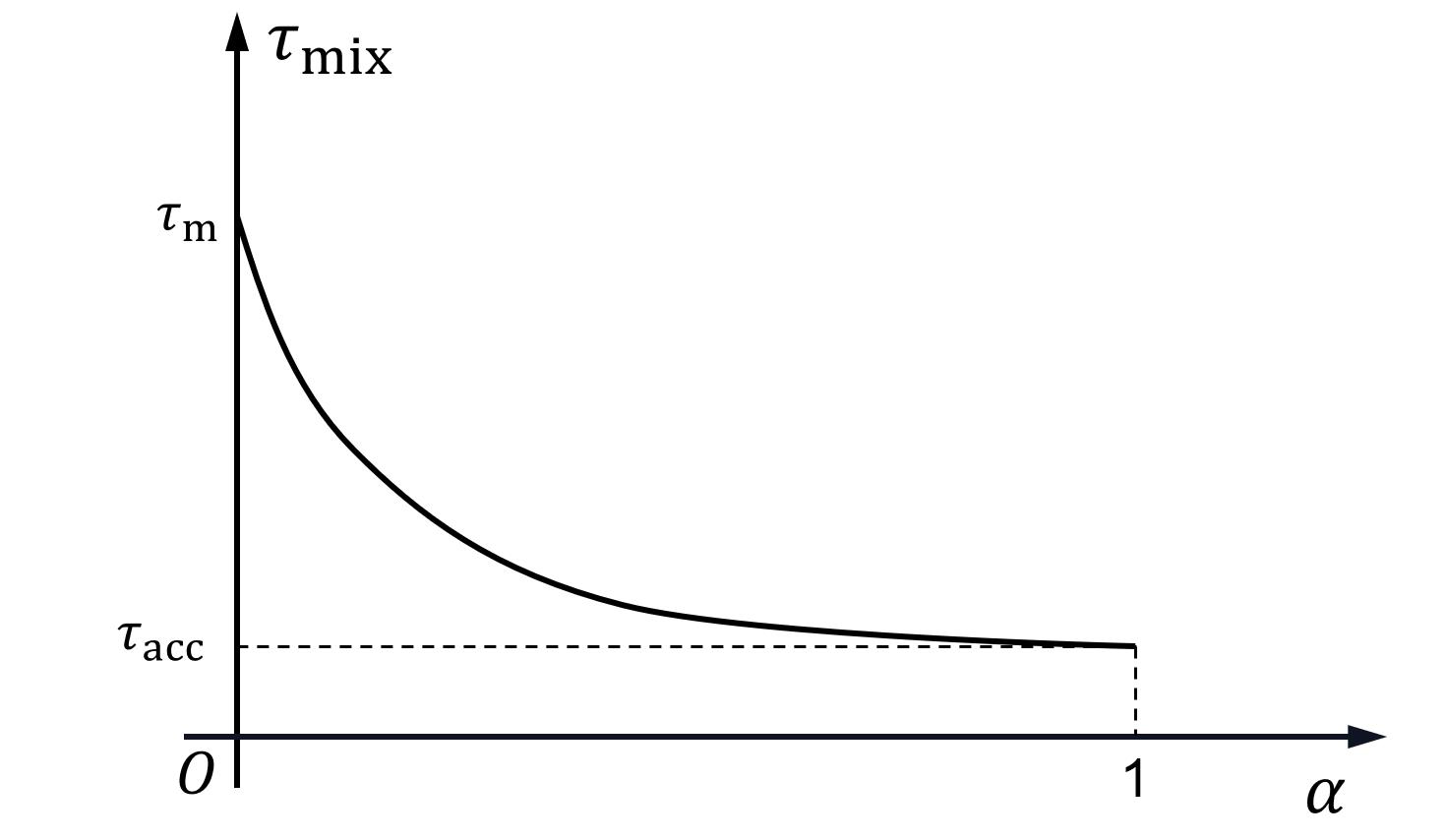
$\tau_{\rm{mix}}$ is also a function of $\alpha$, the percentage of ACC vehicles with respect to total vehicles. Fig. 1 shows the relations of these two parameters. The equilibrium speed profile of the mixed flow $V_{\rm{mix}}$ is expressed as

$$V_{\rm{mix}}(\breve{\rho},\breve{h}_{\rm{acc}})= \frac{1}{\breve{h}_{\rm{mix}}(\breve{h}_{\rm{acc}})}\left(\frac{1}{\breve{\rho}}-l\right),$$ (6)

and the mixed time gap is defined as

$$\breve{h}_{\rm{mix}}(\breve{h}_{\rm{acc}})= \frac{\alpha+(1-\alpha)\frac{\tau_{\rm{acc}}}{\tau_{\rm{m}}}}{\alpha+(1-\alpha)\frac{\tau_{\rm{acc}}}{\tau_{\rm{m}}}\frac{\breve{h}_{\rm{acc}}}{\breve{h}_{\rm{m}}}}\breve{h}_{\rm{acc}}.$$ (7)

In the above model, $l>0$ denotes the average effective vehicle length, $q_{\rm{in}}>0$ is a constant external inflow, and $\breve{h}_{\rm{m}}>0$ is the time gap of manual vehicles.

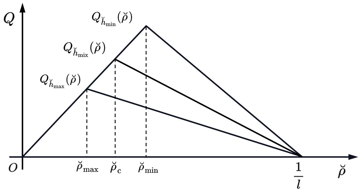
Equation (1) means that the traffic flow observe the mass conservation law [16]. Equation (2) is a momentum equation inspired by the speed dynamics of ARZ model [36] for ACC-equipped and manual mixed flow, where $\alpha\in[0,1]$ is the percentage of ACC vehicles with respect to total vehicles. In (2), $V_{\mathrm{mix}}(\breve{\rho},\breve{h}_{\rm{acc}})=Q(\breve{\rho},\breve{h}_{\rm{acc}})/\breve{\rho}$ is the equilibrium speed profile of a mixed flow of ACC vehicles and manual vehicles, where $Q(\breve{\rho},\breve{h}_{\rm{acc}})$ is the traffic flow given by the fundamental diagram shown in Fig. 2. Define $\breve{\rho}_{c}$ as the lowest density value of the mixed time gap $\breve{h}_{\rm{mix}}$, for which the traffic is congested. Let $\breve{h}_{\rm{min}}$ and $\breve{h}_{\rm{max}}$ be the minimum and maximum possible time gap, namely, $\breve{h}_{\rm{min}}\leq\min\{\breve{h}_{\rm{acc}},\breve{h}_{\rm{m}}\}$ and $\breve{h}_{\rm{max}}\geq\max\{\breve{h}_{\rm{acc}},\breve{h}_{\rm{m}}\}$. Define $\breve{\rho}_{\rm{min}}$ and $\breve{\rho}_{\rm{max}}$ as the lowest density values of congested traffic that correspond to minimum and maximum possible time gaps $\breve{h}_{\rm{min}}$ and $\breve{h}_{\rm{max}}$, respectively. From Fig. 2. we find $Q_{\breve{h}_{\rm{min}}}(\breve{\rho}_{\rm{min}})=v_{\rm{f}}\breve{\rho}_{\rm{min}}$ is the maximal flow at given time gap $\breve{h}_{\rm{mix}}\in[\breve{h}_{\rm{min}},~{}\breve{h}_{\rm{max}}]$. If $\breve{\rho}\geq\breve{\rho}_{\rm{min}}$, implying that the traffic is in congested state, we have

$$Q_{\breve{h}_{\rm{mix}}}(\breve{\rho})=(1-l\breve{\rho})\frac{v_{\rm{f}}}{1/\breve{\rho}_{\rm{c}}-l}.$$ (8)

Combined with (6), we get

$$Q_{\breve{h}_{\rm{mix}}}(\breve{\rho},\breve{h}_{\rm{acc}})=\breve{\rho}V_{\rm{mix}}=(1-l\breve{\rho}) \frac{1}{\breve{h}_{\rm{mix}}(\breve{h}_{\rm{acc}})},$$ (9)

which gives

$$\breve{h}_{\rm{mix}}(\breve{h}_{\rm{acc}})=\frac{1/\breve{\rho}_{\rm{c}}-l}{v_{\rm{f}}}.$$ (10)

Fig. 2: Fundamental diagrams for $\breve{h}_{\rm{mix}}\in[\breve{h}_{\rm{min}},\breve{h}_{\rm{max}}]$.

In other words, for each input $\breve{h}_{\rm{mix}}$, there is a corresponding $\breve{\rho}_{\rm{c}}$, such as $\breve{\rho}_{\rm{min}}=\frac{1}{\breve{h}_{\rm{min}}v_{\rm{f}}+l}$, which guarantees $0<V_{\rm{mix}}(\breve{\rho},\breve{h}_{\rm{acc}})\leq v_{\rm{f}}$. Fig. 2 shows that possible flow $Q_{\breve{h}{\rm{mix}}}(\breve{\rho})$ for every $\breve{h}_{\rm{mix}}\in[\breve{h}_{\rm{min}},~{}\breve{h}_{\rm{max}}]$ lies between $Q_{\breve{h}{\rm{max}}}(\breve{\rho})$ and $Q_{\breve{h}{\rm{min}}}(\breve{\rho})$. In congested regime, we define the feasible set of the state and input variables: $\Phi=\{(\breve{v},\breve{\rho},~{}\breve{h}_{\rm{acc}})\in\mathbb{R}^{3},~{}0\leq\breve{v}\leq v_{\rm{f}},~{}\breve{\rho}_{\rm{min}}\leq\breve{\rho}\leq 1/l,~{}\breve{h}_{\rm{min}}\leq\breve{h}_{\rm{acc}}\leq\breve{h}_{\rm{max}}\}$, for all $\alpha\in[0,1]$.

Using an analysis method similar to the one employed in [36], one can find that system (1)-(4) is anisotropic.

II-B Linearization of the ARZ model

Consider the same equilibria of system (1)-(4) as in [4], dictated by a constant inflow $q_{\rm{in}}$ and a constant, steady-state time gap $\bar{h}_{\rm{acc}}$ for ACC vehicles, which results in the following steady-state traffic speed and density:

$$\bar{v}=\frac{l}{(1/q_{\rm{in}})-\bar{h}_{\rm{mix}}},~{}~{}~{}\bar{\rho}=\frac{1}{l+\bar{h}_{\rm{mix}}\bar{v}},$$ (11)

with mixed time gap

$$\bar{h}_{\rm{mix}}= \frac{\alpha+(1-\alpha)\frac{\tau_{\rm{acc}}}{\tau_{\rm{m}}}}{\alpha+(1-\alpha)\frac{\tau_{\rm{acc}}}{\tau_{\rm{m}}}\frac{\bar{h}_{\rm{acc}}}{\breve{h}_{\rm{m}}}}\bar{h}_{\rm{acc}}.$$ (12)

We define the error variables

$$\rho(x,t) =\breve{\rho}(x,t)-\bar{\rho},$$

$$v(x,t) =\breve{v}(x,t)-\bar{v},$$

$${h}_{\rm{acc}}(x,t) =\breve{h}_{\rm{acc}}(x,t)-\bar{h}_{\rm{acc}}.$$

Linearizing (1)-(4) around the equilibrium (11) and (12), we get

$$\rho_{t}(x,t) =-\bar{v}\rho_{x}(x,t)-\bar{\rho}v_{x}(x,t),$$ (13)

$$v_{t}(x,t) =\frac{l}{\bar{h}_{\rm{mix}}}v_{x}(x,t)-\frac{1}{\bar{\rho}^{2}\tau_{\rm{mix}}\bar{h}_{\rm{mix}}}\rho(x,t)-\frac{1}{\tau_{\rm{mix}}}v(x,t)$$

$$~{}~{}~{}-\frac{\alpha(1-l\bar{\rho})}{\tau_{\rm{acc}}\bar{h}_{\rm{acc}}^{2}\bar{\rho}}h_{\rm{acc}}(x,t-D),$$ (14)

$$\rho(0,t) =-\frac{\bar{\rho}}{\bar{v}}v(0,t),$$ (15)

$$v_{t}(L,t) =-\frac{1}{\bar{\rho}^{2}\tau_{\rm{mix}}\bar{h}_{\rm{mix}}}\rho(L,t)-\frac{1}{\tau_{\rm{mix}}}v(L,t)$$

$$-\frac{\alpha(1-l\bar{\rho})}{\tau_{\rm{acc}}\bar{h}_{\rm{acc}}^{2}\bar{\rho}}h_{\rm{acc}}(L,t-D).$$ (16)

Introducing a change of variable

$${z}(x,t)=\mathrm{e}^{\frac{x}{\bar{v}\tau_{\rm{mix}}}}({\rho}(x,t)+\bar{h}_{\rm{mix}}\bar{\rho}^{2}{v}(x,t)),$$ (17)

and denoting the input by $u(x,t)=h_{\rm{acc}}(x,t)$, we obtain a $2\times 2$ first-order hyperbolic linear PDE system in a diagonal form

$$z_{t}(x,t) =-c_{1}z_{x}(x,t)-\mathrm{e}^{c_{2}x}c_{3}u(x,t-D),$$ (18)

$$v_{t}(x,t) =c_{4}v_{x}(x,t)-c_{5}\mathrm{e}^{-c_{2}x}z(x,t)-c_{6}u(x,t-D),$$ (19)

$$z(0,t) =-c_{7}v(0,t),$$ (20)

$$v_{t}(L,t) =-c_{5}\mathrm{e}^{-c_{2}L}z(L,t)-c_{6}u(L,t-D),$$ (21)

$$z(x,0) =z_{0}(x),~{}~{}v(x,0)=v_{0}(x),$$ (22)

$$u(x,s-D) =\vartheta_{0}(x,s),~{}~{}~{}~{}s\in[0,D],$$ (23)

where $c_{1}=\bar{v}$, $c_{2}=\frac{1}{\tau_{\rm{mix}}\bar{v}}$, $c_{3}=\frac{\alpha\bar{h}_{\rm{mix}}\bar{\rho}^{2}}{\tau_{\rm{acc}}\bar{h}_{\rm{acc}}^{2}}((1/\bar{\rho})-l)$, $c_{4}=\frac{l}{\bar{h}_{\rm{mix}}}$, $c_{5}=\frac{1}{\bar{\rho}^{2}\tau_{\rm{mix}}\bar{h}_{\rm{mix}}}$, $c_{6}=\frac{\alpha}{\tau_{\rm{acc}}\bar{h}_{\rm{acc}}^{2}}((1/\bar{\rho})-l)$, $c_{7}=\frac{l\bar{\rho}^{2}}{\bar{v}}$, and one can easily find the equivalence relation of the coefficients: $c_{2}c_{4}=c_{5}c_{7}$ and $c_{1}c_{2}=\frac{c_{3}c_{5}}{c_{6}}$. The initial conditions is defined in (22). The initial actuator state, i.e., the control memory in $[0,D],$ is denoted by $\vartheta_{0}(x,s)\in L_{2}([0,L]\times[0,D])$ in (23).

Before we proceed, we make the following assumption on the coefficients:

Assumption 1.

Assume $(c_{1}+c_{4})D<L$, which gives $(c_{1}+c_{4})s<L$ for all $0\leq s\leq D$.

Remark 1.

The assumption is reasonable for the traffic application, because the length of the concerned highway stretch $L$ is usually far greater than the other parameters, such that $(c_{1}+c_{4})D$ (delay $D$ times the sum of steady speed $c_{1}=\bar{v}$ and vehicle length $l$ over mixed time gap $\bar{h}_{\rm{mix}}$, $c_{4}=\frac{l}{\bar{h}_{\rm{mix}}}$) much less than $L$.

Our goal is to find a control $u(x,t)$ that exponentially stabilizes the linearized system (18)-(23) with input delay. In the next section, we present the control design.

III Predictor-Feedback Control Design

Before we apply the PDE backstepping approach to the linearized model (18)-(23) with input delay, we first introduce a 2D transport PDE representation of the delay on the 1D-distributed input:

$$z_{t}(x,t)= -c_{1}z_{x}(x,t)-\mathrm{e}^{{c}_{2}x}c_{3}\psi(x,0,t),$$ (24)

$$v_{t}(x,t)= c_{4}v_{x}(x,t)-c_{5}\mathrm{e}^{-{c}_{2}x}z(x,t)-c_{6}\psi(x,0,t),$$ (25)

$$z(0,t)= -{c}_{7}v(0,t),$$ (26)

$$v_{t}(L,t)= \dot{-}c_{5}\mathrm{e}^{-c_{2}L}z(L,t)-c_{6}\psi(L,0,t),$$ (27)

$$\psi_{t}(x,s,t)= \psi_{s}(x,s,t),$$ (28)

$$\psi(x,D,t)= u(x,t),$$ (29)

$$\psi(x,s,0)= \vartheta_{0}(x,s).$$ (30)

From the last three equations, we have

$$\psi(x,s,t)=\begin{cases}u(x,t+s-D)&s+t>D\\ \vartheta(x,t+s)&s+t\leq D\\ \end{cases}.$$ (31)

III-A Backstepping transformation

To design a stabilizing controller for the PDE-ODE system (24)-(29) one has to understand first both its open-loop structure and its actuation structure. Physically speaking, there are three transport processes. Two of the transport processes are in 1D and one is in 2D. One 1D transport is in the $x$ direction at speed $c_{1}$ in (24). The other 1D transport is in the $-x$ direction at speed $c_{4}$ in (25). The two 1D transports create a $(z,v)$ PDE feedback loop, which may be unstable. The 2D transport is in the $-s$ direction at unity speed (and stagnant in the $x$ direction) in (28).

The $z(x,t)$ term in (25) creates a potentially destabilizing feedback loop but is matched by the actuated term $\psi(x,0,t)$. Likewise, the $z(L,t)$ term in (27) creates a potentially destabilizing feedback loop but is matched by the actuated term $\psi(L,0,t)$. These two observations motivate the choice of a target system as

$${z}_{t}(x,t)= -c_{1}{z}_{x}(x,t)+c_{1}c_{2}z(x,t)-c_{3}\mathrm{e}^{c_{2}x}\beta(x,0,t)$$

$$-\frac{kc_{3}}{c_{6}}\mathrm{e}^{c_{2}x}v(x,t),$$ (32)

$${v}_{t}(x,t)= c_{4}{v}_{x}(x,t)-c_{6}\beta(x,0,t)-kv(x,t),$$ (33)

$${z}(0,t)= -c_{7}v(0,t),$$ (34)

$$v_{t}(L,t)= -kv(L,t)-c_{6}\beta(L,0,t),$$ (35)

$$\beta_{t}(x,s,t)= \beta_{s}(x,s,t),$$ (36)

$$\beta(x,D,t)= 0,$$ (37)

where $k>0$ is a free parameter which can be used to set the desired rate of stability.

Remark 2.

The dynamic equation (27) and (35) on the boundary are not standard boundary conditions, which implies that the hyperbolic PDE (24)-(29) and (III-A)–(37) are both preceded by an ODE whose state is $v(L,t)$. Introducing an additional one-dimensional state $X(t)\in\mathbb{R}$ and $Y(t)\in\mathbb{R}$ for (27) and (35), respectively, one can rewrite (27) as:

$$\dot{X}= -c_{5}\mathrm{e}^{-c_{2}L}z(L,t)-c_{6}\psi(L,0,t),$$ (38)

$$v(L,t)= X(t).$$ (39)

and (35) as:

$$\dot{Y}= -kY(L,t)-c_{6}\beta(L,0,t),$$ (40)

$$v(L,t)= Y(t).$$ (41)

Since the additional ODEs are relatively simple, we directly use the boundary values $v(L,t)$ and $v_{t}(L,t)$ in the following computation for notational brevity. Introduce the following transformation

$$\beta(x,s,t)=\psi(x,s,t)+\int_{0}^{L}\gamma(x,s,y){z}(y,t)dy$$

$$+\int_{0}^{L}\eta(x,s,y){v}(y,t)dy+\mathfrak{r}(x,s){v}(L,t)$$

$$+\int_{0}^{L}\int_{0}^{s}G(x,s,y,r)\psi(y,r,t)drdy,$$ (42)

where $\gamma(\cdot,\cdot,\cdot)$, $\eta(\cdot,\cdot,\cdot)$, $G(x,s,y,r)$ and $\mathfrak{r}(\cdot,\cdot)$ are kernel functions defined on $\mathcal{T}_{1}=\{[0,L]\times[0,D]\times[0,L]\}$, $\mathcal{T}_{2}=\{(x,s,y,r)|[0,L]\times[0,D]\times[0,L]\times[0,s]\}$ and $\mathcal{T}_{3}=\{[0,L]\times[0,D]\}$, respectively. Mapping original system (24)–(30) to target system (III-A)–(37) by transformation (42), one can get the following equations of $\mathfrak{r}$:

$$\mathfrak{r}_{s}(x,s)= c_{4}\eta(x,s,L),$$ (43)

$$\mathfrak{r}(x,0)= 0,$$ (44)

which gives

$$\mathfrak{r}(x,s)= \int_{0}^{s}c_{4}\eta(x,\theta,L)d\theta,$$ (45)

and equations of $\gamma$ and $\eta$, respectively:

$$\gamma_{s}(x,s,y)-c_{1}\gamma_{y}(x,s,y)= -c_{5}\mathrm{e}^{-{c}_{2}y}\eta(x,s,y),$$ (46)

$$\eta_{s}(x,s,y)+c_{4}\eta_{y}(x,s,y)= ~{}0,$$ (47)

$$\gamma(x,s,L)= -\frac{c_{5}}{c_{1}}\mathrm{e}^{-{c}_{2}L}\mathfrak{r}(x,s),$$ (48)

$$\gamma(x,0,y)= -\frac{c_{5}}{c_{6}}\mathrm{e}^{-{c}_{2}x}\delta(x-y),$$ (49)

$$\eta(x,s,0)= -\frac{c_{1}c_{7}}{c_{4}}\gamma(x,s,0),$$ (50)

$$\eta(x,0,y)= \frac{k}{c_{6}}\delta(x-y).$$ (51)

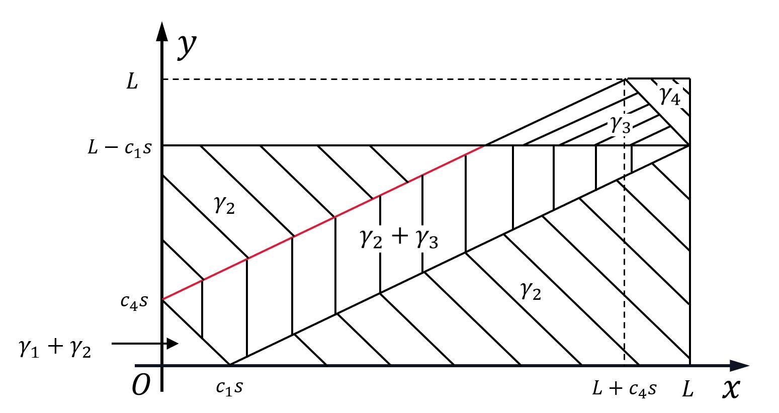
Fig. 3: The regions of kernel $\gamma(x,s,y)$.

Under Assumption 1, we solve kernel $\gamma(\cdot,\cdot,\cdot)$ and $\eta(\cdot,\cdot,\cdot)$ by using the characteristic line method and the successive approximations method (more details please see Appendix A) and get:

$$\gamma (x,s,y)=\gamma_{1}(x,s,y)+\gamma_{2}(x,s,y),$$ (52a)

$$~{}~{}\mathrm{if}~{}0\leq y\leq c_{4}(s-\frac{x}{c_{1}});$$

$$\gamma (x,s,y)=\gamma_{2}(x,s,y),$$ (52b)

$$~{}~{}\mathrm{if}~{}x+c_{4}s<y\leq L-c_{1}s~{}\mathrm{or}~{}0\leq y\leq x-c_{1}s;$$

$$\gamma (x,s,y)=\gamma_{3}(x,s,y),$$ (52c)

$$~{}~{}\mathrm{if}~{}L-c_{1}s<y\leq\min\{x+c_{4}s,\frac{c_{1}+c_{4}}{c_{4}}L-\frac{c_{1}}{c_{4}}x-c_{1}s\};$$

$$\gamma (x,s,y)=\gamma_{2}(x,s,y)+\gamma_{3}(x,s,y),$$ (52d)

$$~{}~{}\mathrm{if}~{}\max\{c_{4}(s-\frac{x}{c_{1}}),x-c_{1}s\}<y$$

$$~{}~{}~{}~{}~{}~{}~{}~{}~{}\leq\min\{x+c_{4}s,L-c_{1}s\};$$

$$\gamma (x,s,y)=\gamma_{4}(x,s,y),$$ (52e)

$$~{}~{}\mathrm{if}~{}\frac{c_{1}+c_{4}}{c_{4}}L-\frac{c_{1}}{c_{4}}x-c_{1}s\leq y\leq L;$$

$$\gamma (x,s,y)=0,~{}~{}\mathrm{otherwise};$$ (52f)

with

$$\gamma_{1}(x,s,y)=-\frac{c_{5}(k+c_{5}c_{7})}{c_{6}(c_{1}+c_{4})}\mathrm{e}^{-c_{2}(x+y)},$$ (53)

$$\gamma_{2}(x,s,y)=-\frac{c_{5}}{c_{6}}\mathrm{e}^{-{c}_{2}x}\delta(x-y-c_{1}s),$$ (54)

$$\gamma_{3}(x,s,y)=-\frac{kc_{5}}{c_{6}(c_{1}+c_{4})}\mathrm{e}^{-\frac{c_{1}c_{2}}{c_{1}+c_{4}}x-\frac{c_{2}c_{4}}{c_{1}+c_{4}}(y+c_{1}s)},$$ (55)

$$\gamma_{4}(x,s,y)=-\frac{kc_{5}}{c_{1}c_{6}}\mathrm{e}^{-c_{2}L}.$$ (56)

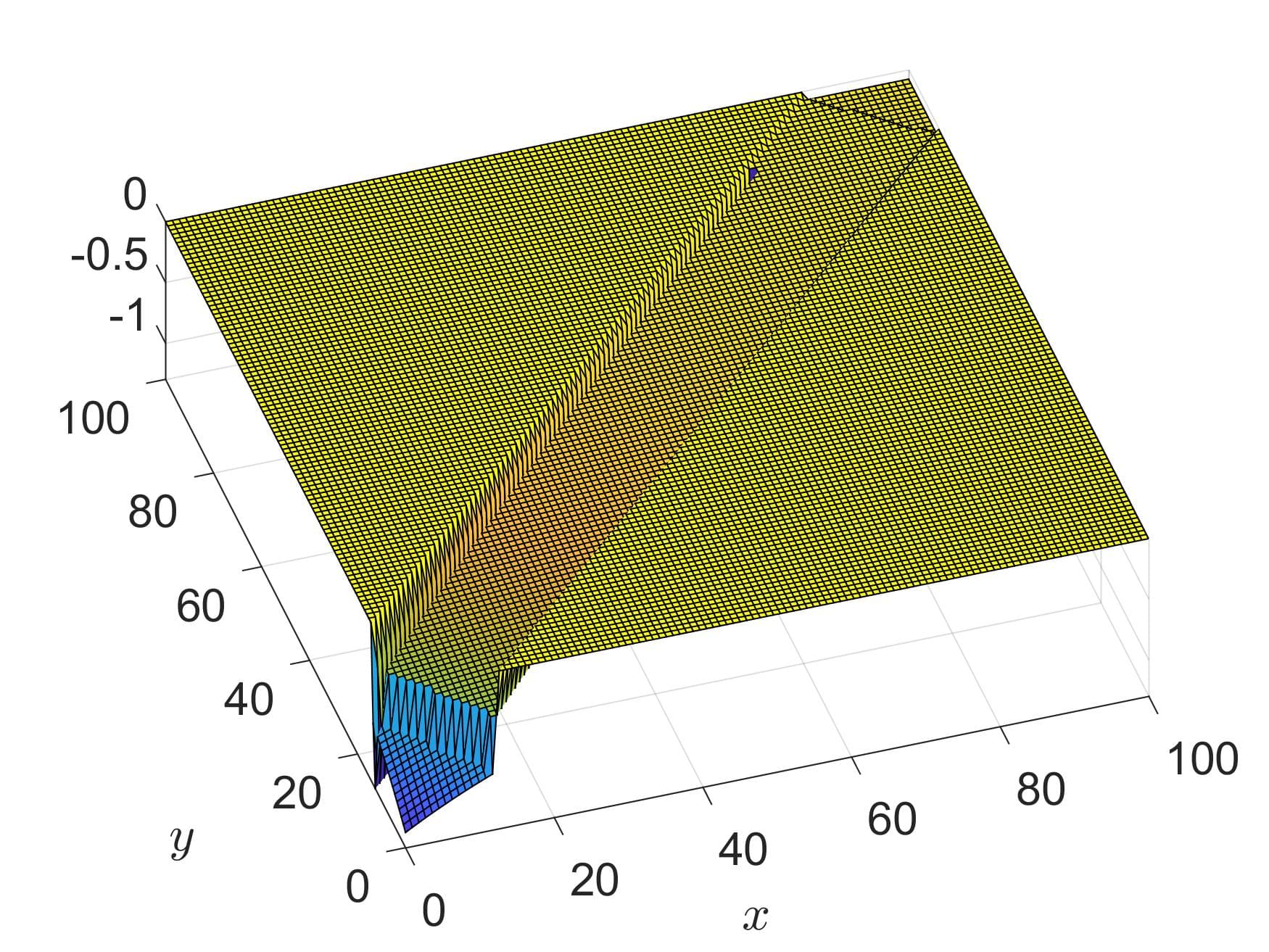
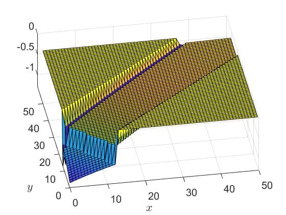
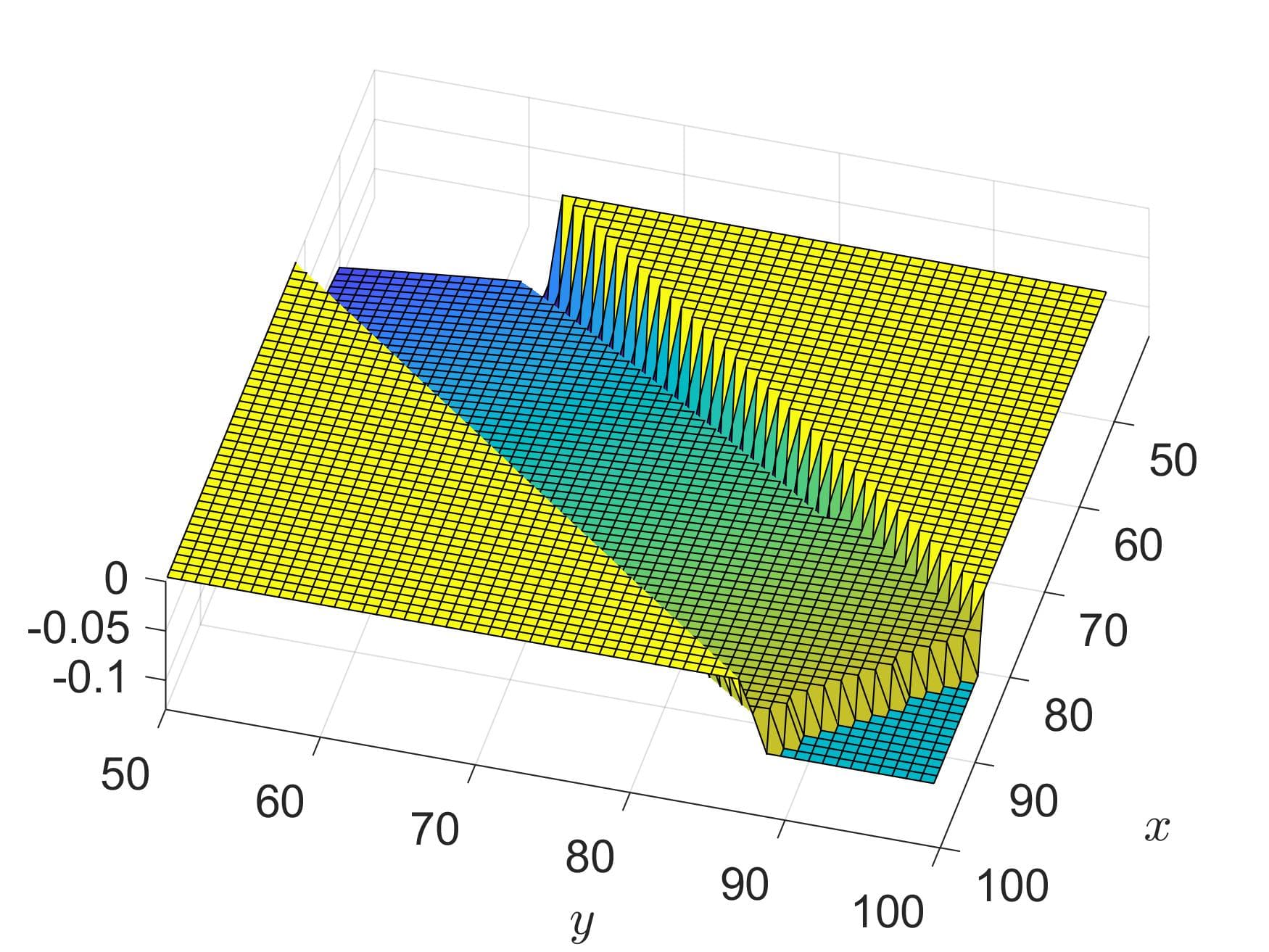
Fig. 4: (a) The kernel function $\gamma(x,s,y)$ with $s=4$ and in domain $(x,y)\in([0,100]\times[0,100])$, (b) the partially zoomed (a) in domain $(x,y)\in([0,50]\times[0,50])$; and (c) the partially zoomed (a) in domain $(x,y)\in([50,100]\times[50,100])$.

Fig. 3 shows all the regions that kernel $\gamma(\cdot,s,\cdot)$ takes different value under a given $s$, in which the red line ($y=x-c_{1}s$) displays where the pulse appears, $\gamma_{2}\neq 0$. The kernel function $\gamma(x,s,y)$ with $s=4$ under parameters $L=100$, $c_{1}=3.1048$, $c_{2}=0.0287$, $c_{3}=0.0023$, $c_{4}=3.5981$, $c_{5}=5.5671$, $c_{6}=0.1438$, $c_{7}=0.0186$, $k=0.1$, is shown in Fig. 4, where we truncate unlimited pulse of Dirac Delta function for clear displaying the kernel function. Similarly, we get

$$\eta (x,s,y)=\eta_{1}(x,s,y)+\eta_{2}(x,s,y),$$ (57a)

$$~{}~{}\mathrm{if}~{}0\leq y\leq c_{4}s-\frac{c_{4}}{c_{1}}x;$$

$$\eta (x,s,y)=\eta_{2}(x,s,y),$$ (57b)

$$~{}~{}\mathrm{if}~{}\max\{c_{4}s-\frac{c_{4}}{c_{1}}x,0\}<y\leq c_{4}s;$$

$$\eta (x,s,y)=\eta_{3}(x,s,y),$$ (57c)

$$~{}~{}\mathrm{if}~{}c_{4}s<y\leq L;$$

$$\eta (x,s,y)=0,~{}\mathrm{otherwise};$$ (57d)

with

$$\eta_{1}(x,s,y)=\frac{c_{1}c_{5}c_{7}(k+c_{5}c_{7})}{c_{4}c_{6}(c_{1}+c_{4})}\mathrm{e}^{-c_{2}x},$$ (58)

$$\eta_{2}(x,s,y)=\frac{c_{1}c_{5}c_{7}}{c_{4}c_{6}}\mathrm{e}^{-c_{2}x}\delta(x-c_{1}s+\frac{c_{1}}{c_{4}}y),$$ (59)

$$\eta_{3}(x,s,y)=\frac{k}{c_{6}}\delta(x-y+c_{4}s).$$ (60)

The equation of $G(\cdot,\cdot,\cdot,\cdot)$ depends on kernel $\gamma(\cdot,\cdot,\cdot)$ and $\eta(\cdot,\cdot,\cdot)$ as follows:

$$G_{s}(x,s,y,r)= -G_{r}(x,s,y,r)=~{}0,$$ (61)

$$G(x,s,y,0)= -c_{3}\mathrm{e}^{-{c}_{2}y}\gamma(x,s,y)-c_{6}\eta(x,s,y)$$

$$-c_{6}\delta(L-y)\mathfrak{r}(x,s),$$ (62)

which is solved

$$G(x,s,y,r)= -c_{3}\mathrm{e}^{-{c}_{2}y}\gamma(x,s-r,y)-c_{6}\eta(x,s-r,y)$$

$$-c_{6}\delta(L-y)\mathfrak{r}(x,s-r).$$ (63)

Substitute the kernel functions (52), (57), (45) and (63) into the transformation (42), which gives an explicit backstepping transformation as follows:

$$\beta(x,s,t)=\begin{cases}&T_{1}[\psi(t)](x,s)+Z_{1}[z(t)](x,s)\\ &~{}+Y_{1}[v(t)](x,s),~{}\mathrm{if}~{}0\leq x\leq c_{1}s,\\ &T_{2}[\psi(t)](x,s)+Z_{2}[z(t)](x,s)\\ &~{}+Y_{2}[v(t)](x,s),~{}\mathrm{if}~{}c_{1}s<x\leq L-c_{4}s,\\ &T_{3}[\psi(t)](x,s)+Z_{3}[z(t)](x,s)\\ &~{}-\frac{k}{c_{6}}v(L,t),~{}\mathrm{if}~{}L-c_{4}s<x\leq L,\\ \end{cases}$$ (64)

where the operators on state $\psi(\cdot,\cdot,t)$ are

$$T_{1} [\psi(t)](x,s)=\psi(x,s,t)$$

$$-\int_{0}^{\frac{x}{c_{1}}}c_{1}c_{2}\mathrm{e}^{-c_{1}c_{2}\tau}\psi(x-c_{1}\tau,s-\tau,t)d\tau$$

$$+\int_{\frac{x}{c_{1}}}^{s}c_{5}c_{7}\mathrm{e}^{-c_{2}x}\psi(c_{4}(\tau-\frac{x}{c_{1}}),s-\tau,t)d\tau$$

$$-\int_{0}^{s}\int_{\max\{x-c_{1}\tau,c_{4}(\tau-\frac{x}{c_{1}})\}}^{x+c_{4}\tau}\mathfrak{g}(x,y,\tau)\psi(y,s-\tau,t)dyd\tau,$$

$$+\int_{0}^{s}k\psi(x+c_{4}\tau,s-\tau,t)d\tau$$ (65)

$$T_{2} [\psi(t)](x,s)=\psi(x,s,t)$$

$$-\int_{0}^{s}c_{1}c_{2}\mathrm{e}^{-c_{1}c_{2}\tau}\psi(x-c_{1}\tau,s-\tau,t)d\tau$$

$$+\int_{0}^{s}k\psi(x+c_{4}\tau,s-\tau,t)d\tau$$

$$-\int_{0}^{s}\int_{x-c_{1}\tau}^{x+c_{4}\tau}\mathfrak{g}(x,y,\tau)\psi(y,s-\tau,t)dyd\tau,$$ (66)

$$T_{3} [\psi(t)](x,s)=\psi(x,s,t)$$

$$-\int_{0}^{s}c_{1}c_{2}\mathrm{e}^{-c_{1}c_{2}\tau}\psi(x-c_{1}\tau,s-\tau,t)r\tau$$

$$+\int_{0}^{\frac{L-x}{c_{4}}}k\psi(x+c_{4}\tau,s-\tau,t)d\tau$$

$$+\int_{\frac{L-x}{c_{4}}}^{s}k\psi(L,s-\tau,t)d\tau$$

$$-\int_{0}^{s}\int_{x-c_{1}\tau}^{\min\{x+c_{4}\tau,\mathfrak{c}(\tau)\}}\mathfrak{g}(x,y,\tau)\psi(y,s-\tau,t)dyd\tau$$

$$-\int_{\frac{L-x}{c_{4}}}^{s}\int_{\mathfrak{c}(\tau)}^{L}kc_{2}\mathrm{e}^{-c_{2}L}\psi(y,s-\tau,t)dyd\tau,$$ (67)

with

$$\mathfrak{g}(x,y,\tau) =\frac{kc_{1}c_{2}}{c_{1}+c_{4}}\mathrm{e}^{-\frac{c_{1}c_{2}}{c_{1}+c_{4}}(x-y+c_{4}\tau)},$$ (68)

$$\mathfrak{c}(\tau) =\frac{c_{1}+c_{4}}{c_{4}}L-\frac{c_{1}}{c_{4}}x-c_{1}\tau.$$ (69)

The operators on state $z(\cdot,t)$ are

$$Z_{1} [z(t)](x,s)=\int_{0}^{c_{4}(s-\frac{x}{c_{1}})}\frac{c_{5}(k+c_{5}c_{7})}{c_{6}(c_{1}+c_{4})}\mathrm{e}^{-c_{2}(x+y)}z(y,t)dy$$

$$+\int_{c_{4}(s-\frac{x}{c_{1}})}^{x+c_{4}s}\mathfrak{k}(x,s)z(y,t)dy,$$ (70)

$$Z_{2} [z(t)](x,s)=\frac{c_{5}}{c_{6}}\mathrm{e}^{-c_{2}x}z(x-c_{1}s,t)$$

$$+\int_{x-c_{1}s}^{x+c_{4}s}\mathfrak{k}(x,s)z(y,t)dy,$$ (71)

$$Z_{3} [z(t)](x,s)=\frac{c_{5}}{c_{6}}\mathrm{e}^{-c_{2}x}z(x-c_{1}s,t)$$ (72)

$$+\int_{\mathfrak{c}(s)}^{L}\frac{kc_{5}}{c_{1}c_{6}}\mathrm{e}^{-c_{2}L}z(y,t)dy+\int_{x-c_{1}s}^{\mathfrak{c}(s)}\mathfrak{k}(x,s)z(y,t)dy$$

with $\mathfrak{k}(x,s)=\frac{kc_{5}}{c_{6}(c_{1}+c_{4})}\mathrm{e}^{-\frac{c_{1}c_{2}}{c_{1}+c_{4}}x-\frac{c_{2}c_{4}(y+c_{1}s)}{c_{1}+c_{4}}}$ . The operators on state $v(\cdot,t)$ are

$$Y_{1}[v(t)](x,s)=-\frac{c_{5}c_{7}}{c_{6}}\mathrm{e}^{-c_{2}x}v(c_{4}(s-\frac{x}{c_{1}}),t)$$

$$~{}~{}~{}~{}-\frac{k}{c_{6}}v(x+c_{4}s,t)$$

$$~{}~{}~{}~{}-\int_{0}^{c_{4}(s-\frac{x}{c_{1}})}\frac{c_{1}c_{5}c_{7}(k+c_{5}c_{7})}{c_{4}c_{6}(c_{1}+c_{4})}\mathrm{e}^{-c_{2}x}v(y,t)dy,$$ (73)

$$Y_{2}[v(t)](x,s)=-\frac{k}{c_{6}}v(x+c_{4}s,t).$$ (74)

Lemma 1.

If Assumption 1 holds, the transformation (64) is bounded and continuous in $x\in[0,L]$, which transforms the original system (24)-(29) into the target system (III-A)-(37).

The proof of Lemma 1 is given in Appendix B.

Remark 3.

The transformation of the plant (24)-(29) to the target system (III-A)-(37) clearly has to be a 2D backstepping transformation due to the 2D nature of the $\psi$-system and the $\beta$-system. But it is not just the dimensionality that shall make this 2D backstepping transformation complex. The reason for its complexity is that the 1D PDE dynamics of $(z,v)$ evolve perpendicular to the direction of the 2D transport dynamics of $\psi$ through which backstepping is performed. The transverse nature of the $(z,v)$-transport relative to the $\beta$-transport, in both the downstream and upstream direction, will make the backstepping transformation $\psi\mapsto\beta$ very complex.

III-B Delay-compensated control

The control is obtained by substituting $s=D$ into transformation (64), applying the boundary conditions (29) and (37), and using the relation (31), we have if $t>D$,

$$u(x,t)= U_{1}[u](x,t)-Z_{1}[z(t)](x,D)$$

$$-Y_{1}[v(t)](x,D),$$ (75a)

$$~{}~{}\mathrm{if}~{}0\leq x\leq c_{1}D,$$

$$u(x,t)= U_{2}[u](x,t)-Z_{2}[z(t)](x,D)$$

$$-Y_{2}[v(t)](x,D),$$ (75b)

$$~{}~{}\mathrm{if}~{}c_{1}D<x\leq L-c_{4}D,$$

$$u(x,t)= U_{3}[u](x,t)-Z_{3}[z(t)](x,DL,\tau)d\tau$$

$$-\frac{k}{c_{6}}v(L,t),$$ (75c)

$$~{}~{}\mathrm{if}~{}L-c_{4}D<x\leq L,$$

where

$$U_{1}[u](x,t)=\int^{t}_{t-\frac{x}{c_{1}}}c_{1}c_{2}\mathrm{e}^{-c_{1}c_{2}(t-\tau)}u(x-c_{1}(t-\tau),\tau)d\tau$$

$$~{}~{}~{}-\int^{t-\frac{x}{c_{1}}}_{t-D}c_{5}c_{7}\mathrm{e}^{-c_{2}x}u(c_{4}(t-\tau-\frac{x}{c_{1}}),\tau)d\tau$$

$$~{}~{}~{}-\int^{t}_{t-D}ku(x+c_{4}(t-\tau),\tau)d\tau$$

$$~{}~{}~{}+\int^{t}_{t-D}\int_{\max\{x-c_{1}(t-\tau),c_{4}(t-\tau-\frac{x}{c_{1}})\}}^{x+c_{4}(t-\tau)}\frac{kc_{1}c_{2}}{c_{1}+c_{4}}$$

$$~{}~{}~{}\times\mathrm{e}^{-\frac{c_{1}c_{2}}{c_{1}+c_{4}}(x-y+c_{4}(t-\tau))}u(y,\tau)dyd\tau,$$ (76)

$$U_{2}[u](x,t)=\int_{t-D}^{t}c_{1}c_{2}\mathrm{e}^{-c_{1}c_{2}(t-\tau)}u(x-c_{1}(t-\tau),\tau)d\tau$$

$$~{}~{}~{}-\int_{t-D}^{t}ku(x+c_{4}(t-\tau),\tau)d\tau$$

$$~{}~{}~{}+\int_{t-D}^{t}\int_{x-c_{1}(t-\tau)}^{x+c_{4}(t-\tau)}\frac{kc_{1}c_{2}}{c_{1}+c_{4}}\mathrm{e}^{-\frac{c_{1}c_{2}}{c_{1}+c_{4}}(x-y+c_{4}(t-\tau))}$$

$$~{}~{}~{}\times u(y,\tau)dyd\tau,$$ (77)

$$U_{3}[u](x,t)=\int_{t-D}^{t}c_{1}c_{2}\mathrm{e}^{-c_{1}c_{2}(t-\tau)}u(x-c_{1}(t-\tau),\tau)d\tau$$

$$~{}~{}~{}-\int^{t}_{t-\frac{L-x}{c_{4}}}ku(x+c_{4}(t-\tau),\tau)d\tau$$

$$~{}~{}~{}+\int_{t-D}^{t}\int_{x-c_{1}(t-\tau)}^{\min\{x+c_{4}(t-\tau),\frac{c_{1}+c_{4}}{c_{4}}L-\frac{c_{1}}{c_{4}}x-c_{1}(t-\tau)\}}\frac{kc_{1}c_{2}}{c_{1}+c_{4}}$$

$$~{}~{}~{}\times\mathrm{e}^{-\frac{c_{1}c_{2}}{c_{1}+c_{4}}(x-y+c_{4}(t-\tau))}u(y,\tau)dyd\tau$$

$$~{}~{}~{}+\int^{t-\frac{L-x}{c_{4}}}_{t-D}\int_{\frac{c_{1}+c_{4}}{c_{4}}L-\frac{c_{1}}{c_{4}}x-c_{1}(t-\tau)}^{L}kc_{2}\mathrm{e}^{-c_{2}L}u(y,\tau)dyd\tau.$$ (78)

It is because of the aforementioned transverse motion of the $(z,v)$-transport relative to the $\psi$-transport that the control law in (75) is given in three distinct forms: from the inlet to $c_{1}D$, from $L-c_{4}D$ to the outlet, and in between. The control (75) is for the linearized and diagonalized system (24)-(29), and the control law for system (1)-(4) around the equilibrium (11) is also required, so we rewrite it as follows: in the case of $t>D$,

$$\breve{h}_{\rm{acc}} (x,t)=\bar{h}_{\rm{acc}}+U_{1}[\breve{h}_{\rm{acc}}-\bar{h}_{\rm{acc}}]-\mathrm{e}^{\frac{c_{2}}{c_{1}}x}Z_{1}[\breve{\rho}-\bar{\rho}](x,D)$$

$$-\bar{h}_{\rm{mix}}\bar{\rho}^{2}Z_{1}[\breve{v}-\bar{v}](x,D)-Y_{1}[\breve{v}-\bar{v}](x,D),$$ (79a)

$$~{}~{}~{}\mathrm{if}~{}0\leq x\leq c_{1}D,$$

$$\breve{h}_{\rm{acc}} (x,t)=\bar{h}_{\rm{acc}}+U_{2}[\breve{h}_{\rm{acc}}-\bar{h}_{\rm{acc}}]-\mathrm{e}^{\frac{c_{2}}{c_{1}}x}Z_{2}[\breve{\rho}-\bar{\rho}](x,D)$$

$$~{}~{}~{}-\bar{h}_{\rm{mix}}\bar{\rho}^{2}Z_{2}[\breve{v}-\bar{v}](x,D)-Y_{2}[\breve{v}-\bar{v}](x,D),$$ (79b)

$$~{}~{}~{}\mathrm{if}~{}c_{1}D<x\leq L-c_{4}D,$$

$$\breve{h}_{\rm{acc}} (x,t)=\bar{h}_{\rm{acc}}+U_{3}[\breve{h}_{\rm{acc}}-\bar{h}_{\rm{acc}}]-\mathrm{e}^{\frac{c_{2}}{c_{1}}x}Z_{3}[\breve{\rho}-\bar{\rho}](x,D)$$

$$~{}~{}~{}-\bar{h}_{\rm{mix}}\bar{\rho}^{2}Z_{3}[\breve{v}-\bar{v}](x,D)-\frac{k}{c_{6}}(\breve{v}(L,t)-\bar{v})$$

$$~{}~{}~{}-\int^{t-\frac{L-x}{c_{4}}}_{t-D}k(\breve{h}_{\rm{acc}}(L,\tau)-\bar{h}_{\rm{acc}})d\tau,$$ (79c)

$$~{}~{}~{}\mathrm{if}~{}L-c_{4}D<x\leq L,$$

Since the transformation (64) is continuous in $x$, both the control (75) for the linearized error system (24)-(29) and the control (79) for the original system (1)-(4) around the equilibrium (11) are continuous in $x$. The control (79) is composed of the feedback of the states and the historical actuator state, which is divided into three parts upon the spatial variable $x$. It implies the ACC vehicles at different position of the highway will apply different time gap strategies. Due to the length of the concerned highway stretch $L$ being far greater than other parameters (Assumption 1), one can find that the first and the last sections are much shorter than the second section. Hence, most ACC vehicles on the highway adopt the second part of control law when they enter the middle interval $c_{1}D<x\leq L-c_{4}D$. In order to control the traffic flow in the interval near the exit of the highway, the feedback of the flow speed $\breve{v}(L,t)$ at the exit is also required due to the dynamic boundary condition.

IV Stability Analysis

In this section, we analyze the stability of the closed-loop system. First, we state the main result concerning exponentially stability.

Theorem 1.

Consider the closed-loop system consisting of plant (24) -(30) with control law (75), if the initial conditions $z(\cdot,0)\in H_{1}[0,L]$, $v(\cdot,0)\in H_{1}[0,L]$, and $\psi(\cdot,\cdot,0))\in L_{2}(0,L)\times H_{1}[0,D]$ are compatible, then the equilibrium $(z(\cdot,\cdot),v(\cdot,\cdot),\psi(\cdot,\cdot,\cdot))\equiv 0$ is exponentially stable in the $L_{2}$ sense, i.e., there exist positive constants $\vartheta$ and $M$ such that the following holds for all $t>0$,

$$\rVert z\rVert^{2}_{L_{2}}+\rVert v\rVert^{2}_{L_{2}}+|v(L,t)|^{2}+\rVert\psi\rVert^{2}_{L_{2}}+\rVert\psi(L,\cdot,t)\rVert^{2}_{L_{2}}$$

$$\leq M\mathrm{e}^{-\vartheta t}\left(\rVert z(\cdot,0)\rVert^{2}_{L_{2}}+|v(\cdot,0)|^{2}+\rVert v(L,0)\rVert^{2}_{L_{2}}\right.$$

$$~{}\left.+\rVert\psi(\cdot,\cdot,0)\rVert^{2}_{L_{2}}+\rVert\psi(L,\cdot,0)\rVert^{2}_{L_{2}}\right).$$ (80)

The proof of the theorem consists of two steps. The first step is to prove the exponential stability of the target system in $L_{2}$ sense, and the second step is to prove the transformation is invertible by obtaining the explicit inverse transformation, which will establish the norm equivalence between the original system and the target system.

IV-A The stability of the target system

Before proceeding, we first define two Lyapunov functions for the original system (24)-(29) and the target system (III-A)-(37), respectively

$$V_{1}(t) =\rVert z\rVert^{2}_{L_{2}}+\rVert v\rVert^{2}_{L_{2}}+|v(L,t)|^{2}+\rVert\psi\rVert^{2}_{L_{2}}+\rVert\psi(L,\cdot,t)\rVert^{2}_{L_{2}},$$ (81)

$$V_{2}(t) =\rVert z\rVert^{2}_{L_{2}}+\rVert v\rVert^{2}_{L_{2}}+|v(L,t)|^{2}+\rVert\beta\rVert^{2}_{L_{2}}+\rVert\beta(L,\cdot,t)\rVert^{2}_{L_{2}}.$$ (82)

Lemma 2.

Consider system (III-A)-(37). If the initial conditions $z(\cdot,0)\in H_{1}[0,L]$, $v(\cdot,0)\in H_{1}[0,L]$, and $\beta(\cdot,\cdot,0))\in L_{2}(0,L)\times H_{1}[0,D]$ are compatibles, then the equilibrium $(z(\cdot,\cdot),v(\cdot,\cdot),\beta(\cdot,\cdot,\cdot))\equiv 0$ of (III-A)-(37) is exponentially stable in the $L_{2}$ sense, i.e., there exist positive constants $\theta$ and $N$ such that the following holds for all $t>0$,

$$\rVert z\rVert^{2}_{L_{2}}+\rVert v\rVert^{2}_{L_{2}}+|v(L,t)|^{2}+\rVert\beta\rVert^{2}_{L_{2}}+\rVert\beta(L,\cdot,t)\rVert^{2}_{L_{2}}$$

$$~{}~{}~{}\leq M\mathrm{e}^{-\theta t}(\rVert z(\cdot,0)\rVert^{2}_{L_{2}}+\rVert v(\cdot,0)\rVert^{2}_{L_{2}}+|v(L,0)|^{2}$$

$$~{}~{}~{}~{}~{}~{}~{}+\rVert\beta(\cdot,\cdot,0)\rVert^{2}_{L_{2}}+\rVert\beta(L,\cdot,0)\rVert^{2}_{L_{2}}).$$ (83)

Proof.

First, define a Lyapunov function for target system (III-A)-(37)

$$V_{0}(t)= \int_{0}^{L}\mathrm{e}^{-\sigma x}{z}^{2}(x,t)dx+k_{2}\int_{0}^{L}\mathrm{e}^{\sigma x}{v}^{2}(x,t)dx$$

$$+k_{3}v^{2}(L,t)+k_{4}\int_{0}^{L}\int_{0}^{D}\mathrm{e}^{\sigma(s+x)}\beta^{2}(x,s,t)dsdx$$

$$+k_{5}\int_{0}^{D}\mathrm{e}^{\sigma s}\beta^{2}(L,s,t)ds,$$ (84)

where $k_{i}$, $\sigma>0$, $i=2,3,4,5$, whose ranges will be determined later.

Differentiating (84) with respect to time, we get

$$\dot{V_{0}}(t)={I}(t)+{II}(t)+{III}(t),$$ (85)

where

$${I}(t)= -2\int_{0}^{L}c_{1}\mathrm{e}^{-\sigma x}z(x,t){z}_{x}(x,t)dx$$

$$2\int_{0}^{L}c_{1}c_{2}\mathrm{e}^{-\sigma x}z^{2}(x,t)dx$$

$$-2\int_{0}^{L}c_{3}\mathrm{e}^{(c_{2}-\sigma)x}z(x,t)\beta(x,0,t)dx$$

$$-2\int_{0}^{L}\frac{kc_{3}}{c_{6}}\mathrm{e}^{(c_{2}-\sigma)x}z(x,t)v(x,t)dx,$$ (86)

$${II}(t)= 2k_{2}\int_{0}^{L}c_{4}e^{\sigma x}v(x,t)v_{x}(x,t)dx$$

$$-2k_{2}\int_{0}^{L}k\mathrm{e}^{\sigma x}{v}^{2}(x,t)dx$$

$$-2k_{2}\int_{0}^{L}c_{6}\mathrm{e}^{\sigma x}v(x,t)\beta(x,0,t)dx$$

$$-k_{3}c_{6}v(L,t)\beta(L,0,t)-2k_{3}kv^{2}(L,t),$$ (87)

$${III}(t)= -k_{4}\sigma\int_{0}^{L}\int_{0}^{D}\mathrm{e}^{\sigma(x+s)}\beta^{2}(x,s,t)dx$$

$$-k_{4}\int_{0}^{L}\mathrm{e}^{\sigma x}\beta^{2}(x,0,t)dx$$

$$-k_{5}\sigma\int_{0}^{D}\mathrm{e}^{\sigma s}\beta^{2}(L,s,t)ds-k_{5}\beta^{2}(L,0,t).$$ (88)

By using Cauchy-Schwarz Inequality, Young’s Inequality and letting $E=\sup_{x\in[0,L]}\{\mathrm{e}^{c_{2}x}\}$, we get

$${I}(t)\leq\frac{2Ekc_{3}}{c_{6}}\int_{0}^{L}\mathrm{e}^{\sigma x}v^{2}dx+c_{1}c_{7}^{2}v^{2}(0,t)$$

$$~{}~{}-\left(c_{1}\sigma-2c_{1}c_{2}-\frac{Ec_{3}}{2}-\frac{Ekc_{3}}{2c_{6}}\right)\int_{0}^{L}\mathrm{e}^{-\sigma x}z^{2}dx$$

$$~{}~{}+2Ec_{3}\int_{0}^{L}\mathrm{e}^{\sigma x}\beta^{2}(x,0,t)dx,$$ (89)

$${II}(t)\leq-k_{2}(c_{4}\sigma-\frac{c_{6}}{2}+2k)\int_{0}^{L}\mathrm{e}^{\sigma x}v^{2}dx-k_{2}c_{4}v^{2}(0,t)$$

$$~{}~{}+2k_{2}c_{6}\int_{0}^{L}\mathrm{e}^{\sigma x}\beta^{2}(x,0,t)dx+\frac{p}{2}k_{3}c_{6}\beta^{2}(L,0,t)$$

$$~{}~{}-(2k_{3}k-\frac{k_{3}c_{6}}{2p}-k_{2}c_{4}\mathrm{e}^{\sigma L})v^{2}(L,t),$$ (90)

where $\int_{0}^{L}\mathrm{e}^{-\sigma x}\beta^{2}(x,0,t)dx\leq\int_{0}^{L}\mathrm{e}^{\sigma x}\beta^{2}(x,0,t)dx$ is used for getting (89) and $p>0$ is a free parameter of Young’s Inequality. Thus, we get

$$\dot{V_{0}}(t)\leq-\left[k_{2}(c_{4}\sigma-\frac{c_{6}}{2}+2k)-\frac{2Ekc_{3}}{c_{6}}\right]\int_{0}^{L}\mathrm{e}^{\sigma x}v^{2}dx$$

$$~{}~{}-\left(c_{1}\sigma-2c_{1}c_{2}-\frac{Ec_{3}}{2}-\frac{Ekc_{3}}{2c_{6}}\right)\int_{0}^{L}\mathrm{e}^{-\sigma x}z^{2}dx$$

$$~{}~{}-k_{4}\sigma\int_{0}^{L}\int_{0}^{D}\mathrm{e}^{\sigma(x+s)}\beta^{2}(x,s,t)dx$$

$$~{}~{}-\left(2k_{3}k-\frac{k_{3}c_{6}}{2p}-k_{2}c_{4}\mathrm{e}^{\sigma L}\right)v^{2}(L,t)$$

$$~{}~{}-\left(k_{4}-2Ec_{3}-2k_{2}c_{6}\right)\int_{0}^{L}\beta^{2}(x,0,t)$$

$$~{}~{}-(k_{2}c_{4}-c_{1}c_{7}^{2})v^{2}(0,t)-k_{5}\sigma\int_{0}^{D}\mathrm{e}^{\sigma s}\beta^{2}(L,s,t)ds$$

$$~{}~{}-(k_{5}-\frac{p}{2}k_{3}c_{6})\beta^{2}(L,0,t).$$ (91)

Choose the parameters as:

$$\begin{cases}\sigma&>2c_{2}+\frac{Ec_{3}}{2c_{1}}+\frac{Ekc_{3}}{2c_{1}c_{6}},\\ p&>\frac{c_{6}}{4k},\\ k_{2}&>\max\{\frac{2Ekc_{3}}{c_{6}(c_{4}\sigma-\frac{c_{6}}{2}+2k)},\frac{c_{1}c_{7}^{2}}{c_{4}}\},\\ k_{3}&>\frac{k_{2}c_{4}\mathrm{e}^{\sigma L}}{2k-\frac{c_{6}}{2p}},\\ k_{4}&>2Ec_{3}+2k_{2}c_{6},\\ k_{5}&>\frac{2k_{3}c_{6}}{p},\end{cases}$$ (92)

such that

$$\dot{V_{0}}(t)\leq-\left[k_{2}(c_{4}\sigma-\frac{c_{6}}{2}+2k)-\frac{2Ekc_{3}}{c_{6}}\right]\int_{0}^{L}\mathrm{e}^{\sigma x}v^{2}dx$$

$$~{}~{}-\left(c_{1}\sigma-2c_{1}c_{2}-\frac{Ec_{3}}{2}-\frac{Ekc_{3}}{2c_{6}}\right)\int_{0}^{L}\mathrm{e}^{-\sigma x}z^{2}dx$$

$$~{}~{}-k_{4}\sigma\int_{0}^{L}\int_{0}^{D}\mathrm{e}^{\sigma(x+s)}\beta^{2}(x,s,t)dx$$

$$~{}~{}-\left[k_{3}(2k-\frac{c_{6}}{2p})-k_{2}c_{4}\mathrm{e}^{\sigma L}\right]v^{2}(L,t)$$

$$~{}~{}-k_{5}\sigma\int_{0}^{D}\mathrm{e}^{\sigma s}\beta^{2}(L,s,t)ds\leq-\vartheta V(t),$$

where

$$\vartheta= \min\{k_{2}(c_{4}\sigma-\frac{c_{6}}{2}+2k)-\frac{2Ekc_{3}}{c_{6}},$$

$$k_{4}\sigma,~{}(c_{1}\sigma-2c_{1}c_{2}-\frac{Ec_{3}}{2}-\frac{Ekc_{3}}{2c_{6}}),~{}$$

$$k_{3}(2k-\frac{c_{6}}{2})-k_{2}c_{4}\mathrm{e}^{\sigma L},~{}k_{5}\sigma\}.$$

Therefore, we get

$$V_{0}(t)\leq V_{0}(0)\mathrm{e}^{-\vartheta t}.$$ (93)

It is obvious that $V_{0}(t)$ defined by (84) is equivalent to $V_{2}$ defined by (82), i.e., there exist positive constants $\varrho_{1}$ and $\varrho_{2}$, such that $\varrho_{1}V_{2}\leq V_{0}\leq\varrho_{2}V_{2}$. Hence, (83) is proved. ∎

IV-B The inverse transformation

Lemma 3.

The transformation (64) is invertible, and whose inverse transformation is

$$\psi(x,s,t)= Q_{1}[\beta(t)](x,s)+R_{1}[v(t)](x,s),$$ (94a)

$$~{}~{}0\leq x<c_{1}s;$$

$$\psi(x,s,t)= Q_{2}[\beta(t)](x,s)+R_{2}[v(t)](x,s)$$

$$+\mathcal{B}[z(t)](x,s),$$ (94b)

$$~{}~{}c_{1}s<x\leq L-c_{4}s;$$

$$\psi(x,s,t)= Q_{3}[\beta(t)](x,s)+R_{3}[v(t)](x,s)$$

$$+\mathcal{B}[z(t)](x,s),$$ (94c)

$$~{}~{}L-c_{4}s<x\leq L;$$

where

$$Q_{1}[\beta(t)](x,s)=\beta(x,s,t)$$

$$~{}~{}~{}-\int_{\frac{x}{c_{1}}}^{s}\int_{c_{4}(\tau-\frac{x}{c_{1}})}^{x+c_{4}\tau}\frac{kc_{1}c_{2}}{c_{1}+c_{4}}\mathrm{e}^{\frac{k(x-y-c_{1}\tau)}{c_{1}+c_{4}}}\beta(y,s-\tau,t)dyd\tau$$

$$~{}~{}~{}-\int_{0}^{\frac{x}{c_{1}}}\int_{x-c_{1}\tau}^{x+c_{4}\tau}\frac{kc_{1}c_{2}}{c_{1}+c_{4}}\mathrm{e}^{\frac{k(x-y-c_{1}\tau)}{c_{1}+c_{4}}}\beta(y,s-\tau,t)dyd\tau$$

$$~{}~{}~{}-\int_{\frac{x}{c_{1}}}^{s}c_{2}c_{4}\mathrm{e}^{k(\frac{x}{c_{1}}-\tau)}\beta(c_{4}(\tau-\frac{x}{c_{1}}),s-\tau,t)d\tau$$

$$~{}~{}~{}+\int^{\frac{x}{c_{1}}}_{0}c_{1}c_{2}\beta(x-c_{1}\tau,s-\tau,t)d\tau$$

$$~{}~{}~{}-\int_{0}^{s}k\mathrm{e}^{-k\tau}\beta(x+c_{4}\tau,s-\tau,t)d\tau,$$ (95)

$$Q_{2}[\beta(t)](x,s)=\beta(x,s,t)$$

$$~{}~{}~{}-\int_{0}^{s}\int_{x-c_{1}\tau}^{x+c_{4}\tau}\frac{kc_{1}c_{2}}{c_{1}+c_{4}}\mathrm{e}^{\frac{k(x-y-c_{1}\tau)}{c_{1}+c_{4}}}\beta(y,s-\tau,t)dyd\tau$$

$$~{}~{}~{}+\int_{0}^{s}c_{1}c_{2}\beta(x-c_{1}\tau,s-\tau,t)d\tau$$

$$~{}~{}~{}-\int_{0}^{s}k\mathrm{e}^{-k\tau}\beta(x+c_{4}\tau,s-\tau,t)d\tau,$$ (96)

$$Q_{3}[\beta(t)](x,s)=\beta(x,s,t)$$

$$~{}~{}~{}-\int_{0}^{s}\int_{x-c_{1}\tau}^{\min\{L,x+c_{4}\tau\}}\frac{kc_{1}c_{2}}{c_{1}+c_{4}}\mathrm{e}^{\frac{k(x-y-c_{1}\tau)}{c_{1}+c_{4}}}$$

$$~{}~{}~{}\times\beta(y,s-\tau,t)dyd\tau$$

$$~{}~{}~{}+\int_{0}^{s}c_{1}c_{2}\beta(x-c_{1}\tau,s-\tau,t)d\tau$$

$$~{}~{}~{}-\int_{\frac{L-x}{c_{4}}}^{s}(c_{1}c_{2}\mathrm{e}^{\frac{k(x-L-c_{1}\tau)}{c_{1}+c_{4}}}-c_{1}c_{2}\mathrm{e}^{-k\tau}+k\mathrm{e}^{-k\tau})$$

$$~{}~{}~{}\times\beta(L,s-\tau,t)d\tau$$

$$~{}~{}~{}-\int_{0}^{\frac{L-x}{c_{4}}}k\mathrm{e}^{-k\tau}\beta(x+c_{4}\tau,s-\tau,t)d\tau,$$ (97)

$$R_{1}[v(t)](x,s)=\frac{c_{2}c_{4}}{c_{6}}\mathrm{e}^{k(\frac{x}{c_{1}}-s)}v(c_{4}(s-\frac{x}{c_{1}}),t)$$

$$~{}~{}~{}+\frac{k}{c_{6}}\mathrm{e}^{-ks}v(x+c_{4}s,t)$$

$$~{}~{}~{}+\int_{c_{4}(s-\frac{x}{c_{1}})}^{x+c_{4}s}\frac{kc_{1}c_{2}}{c_{6}(c_{1}+c_{4})}\mathrm{e}^{\frac{k(x-y-c_{1}s)}{c_{1}+c_{4}}}v(y,t)dy,$$ (98)

$$R_{2}[v(t)](x,s)=\frac{k}{c_{6}}\mathrm{e}^{-ks}v(x+c_{4}s,t)$$

$$~{}~{}~{}+\int_{x-c_{1}s}^{x+c_{4}s}\frac{kc_{1}c_{2}}{c_{6}(c_{1}+c_{4})}\mathrm{e}^{\frac{k(x-y-c_{1}s)}{c_{1}+c_{4}}}v(y,t)dy,$$ (99)

$$R_{3}[v(t)](x,s)=\int_{x-c_{1}s}^{L}\frac{kc_{1}c_{2}}{c_{6}(c_{1}+c_{4})}\mathrm{e}^{\frac{k(x-y-c_{1}s)}{c_{1}+c_{4}}}v(y,t)dy$$

$$~{}~{}~{}+\left(\frac{c_{1}c_{2}}{c_{6}}\mathrm{(e}^{\frac{k(x-L-c_{1}s)}{c_{1}+c_{4}}}-\mathrm{e}^{-ks})+\frac{k}{c_{6}}\mathrm{e}^{-ks}\right)v(L,t),$$ (100)

$$\mathcal{B}[z(t)](x,s)=-\frac{c_{5}}{c_{6}}\mathrm{e}^{c_{2}(c_{1}s-x)}z(x-c_{1}s,t).$$ (101)

The inverse transformation is bounded and continuous in $x\in[0,L]$.

The proof of Lemma 3 is similar to the proof of Lemma 1, so we will omit the proof due to limited space.

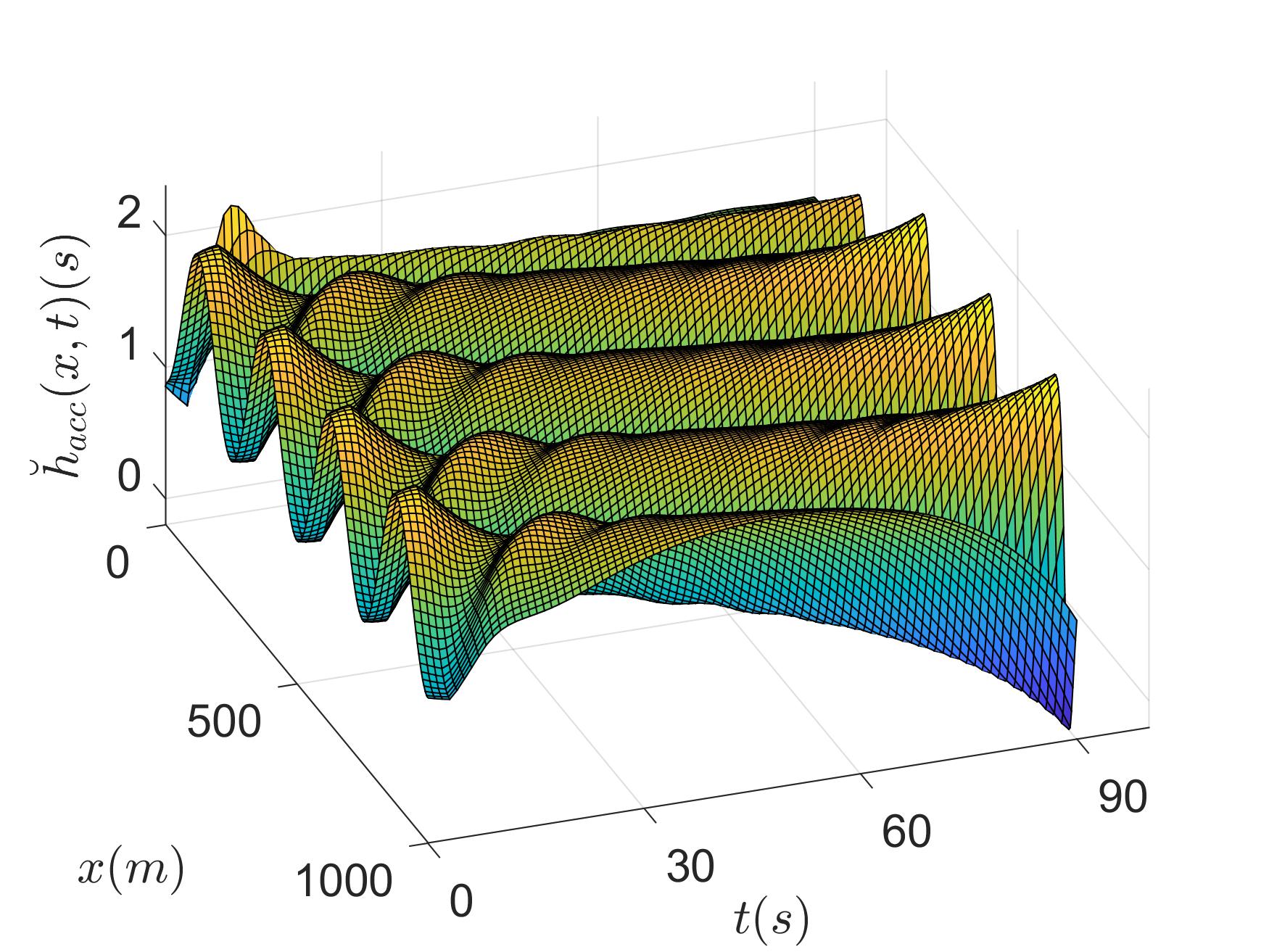
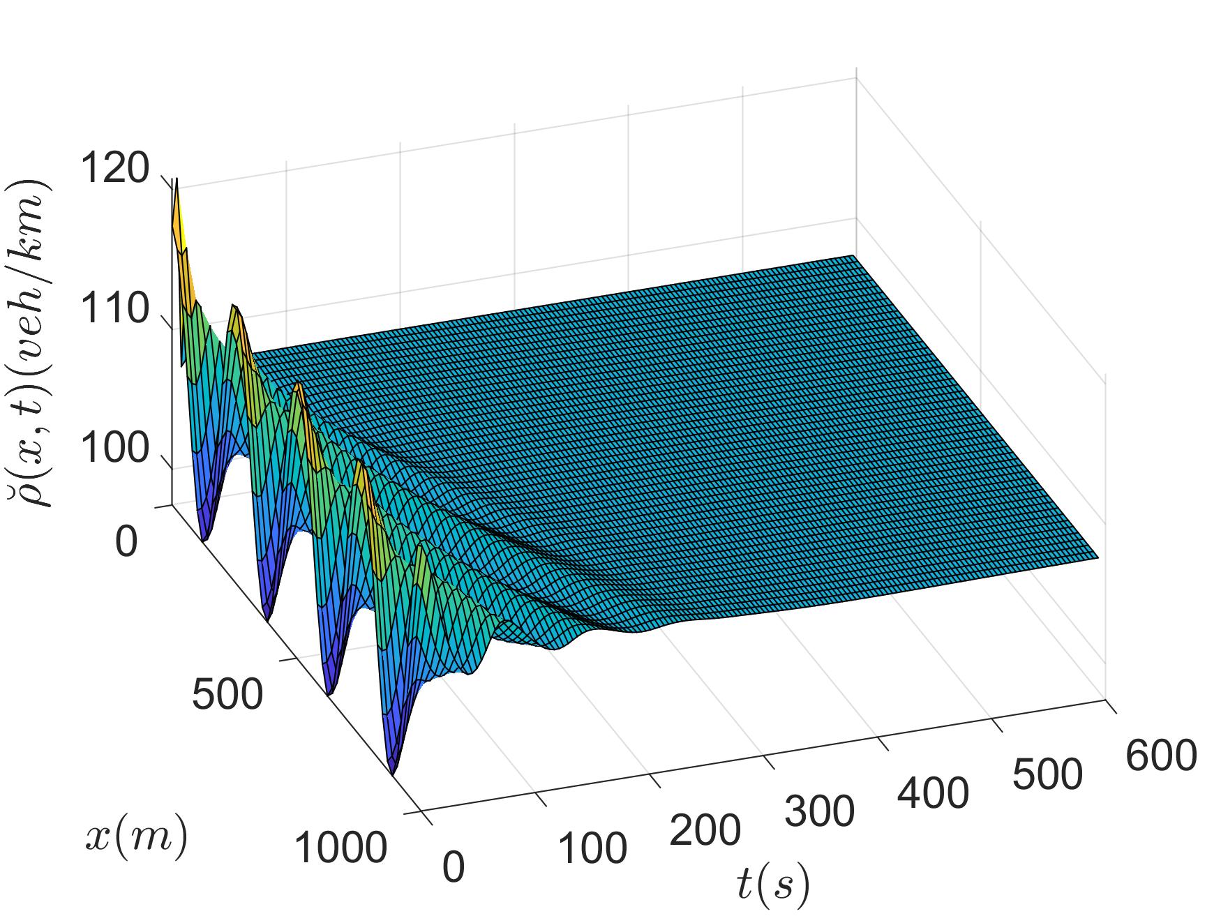
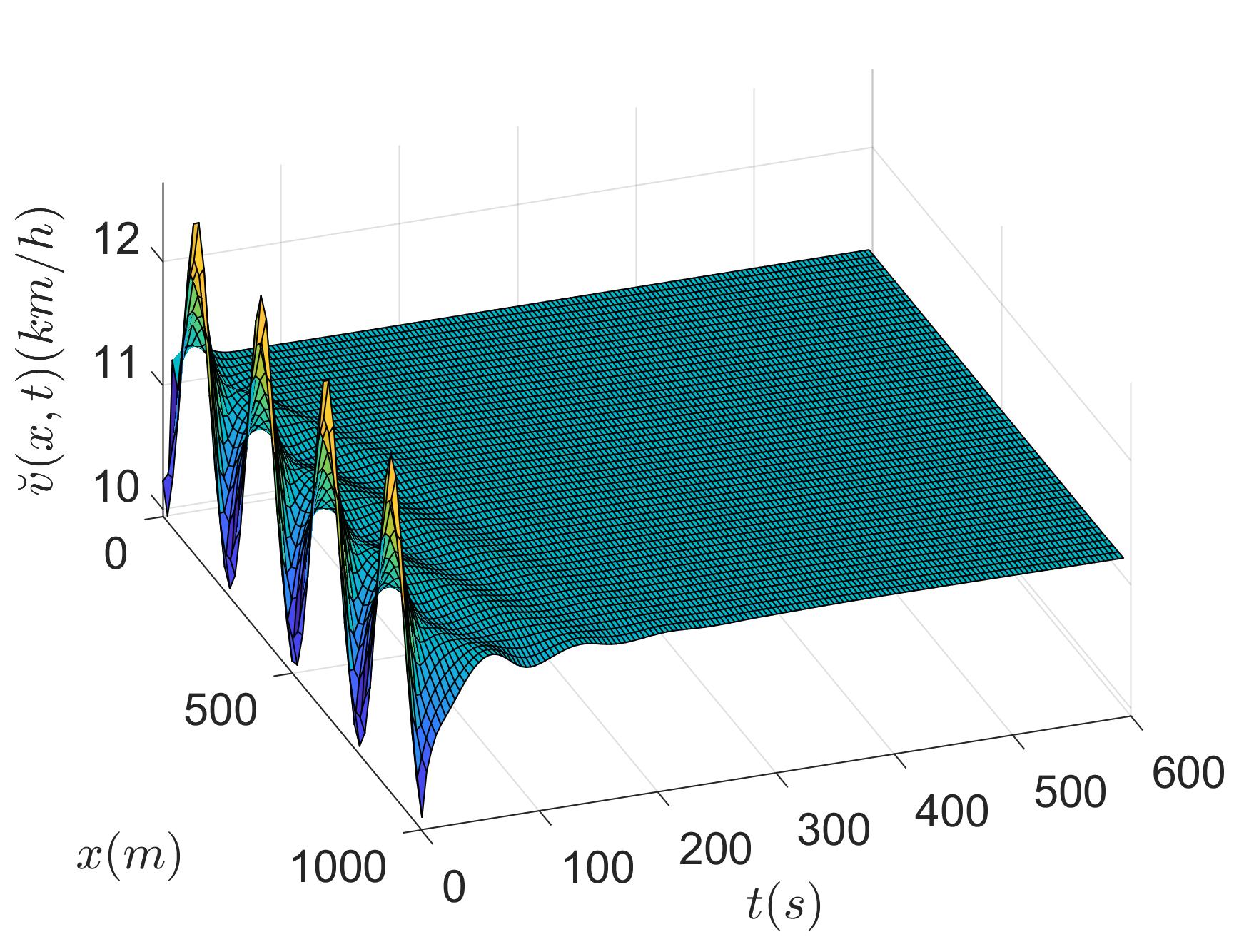
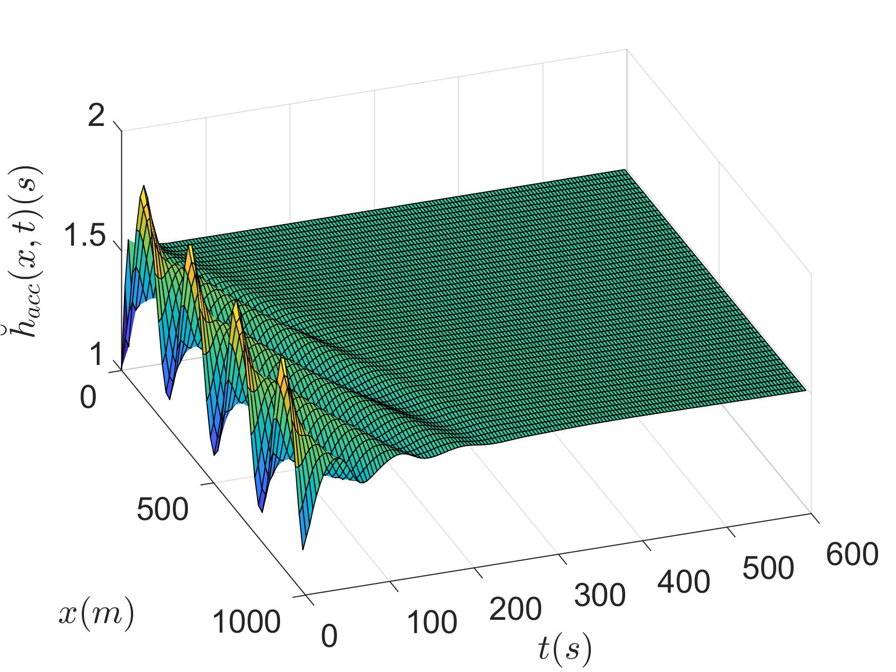
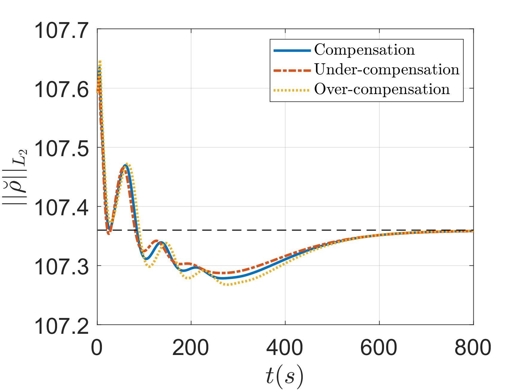
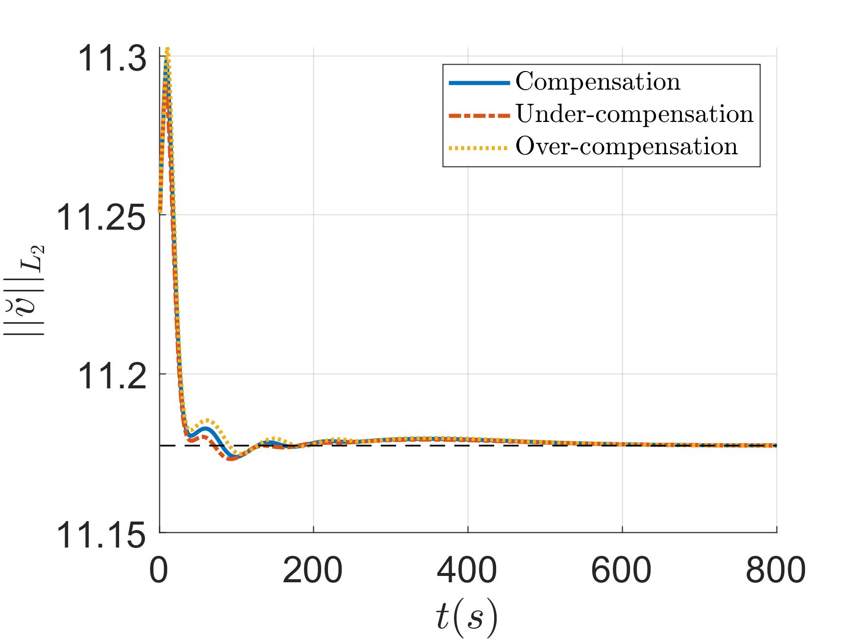
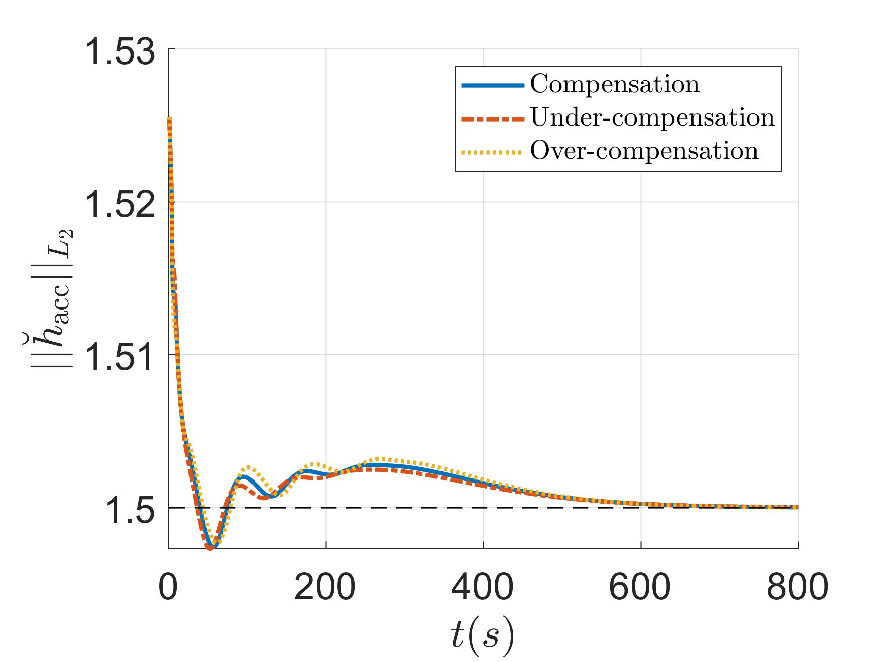
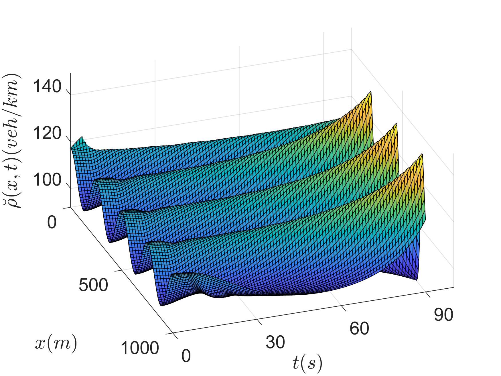
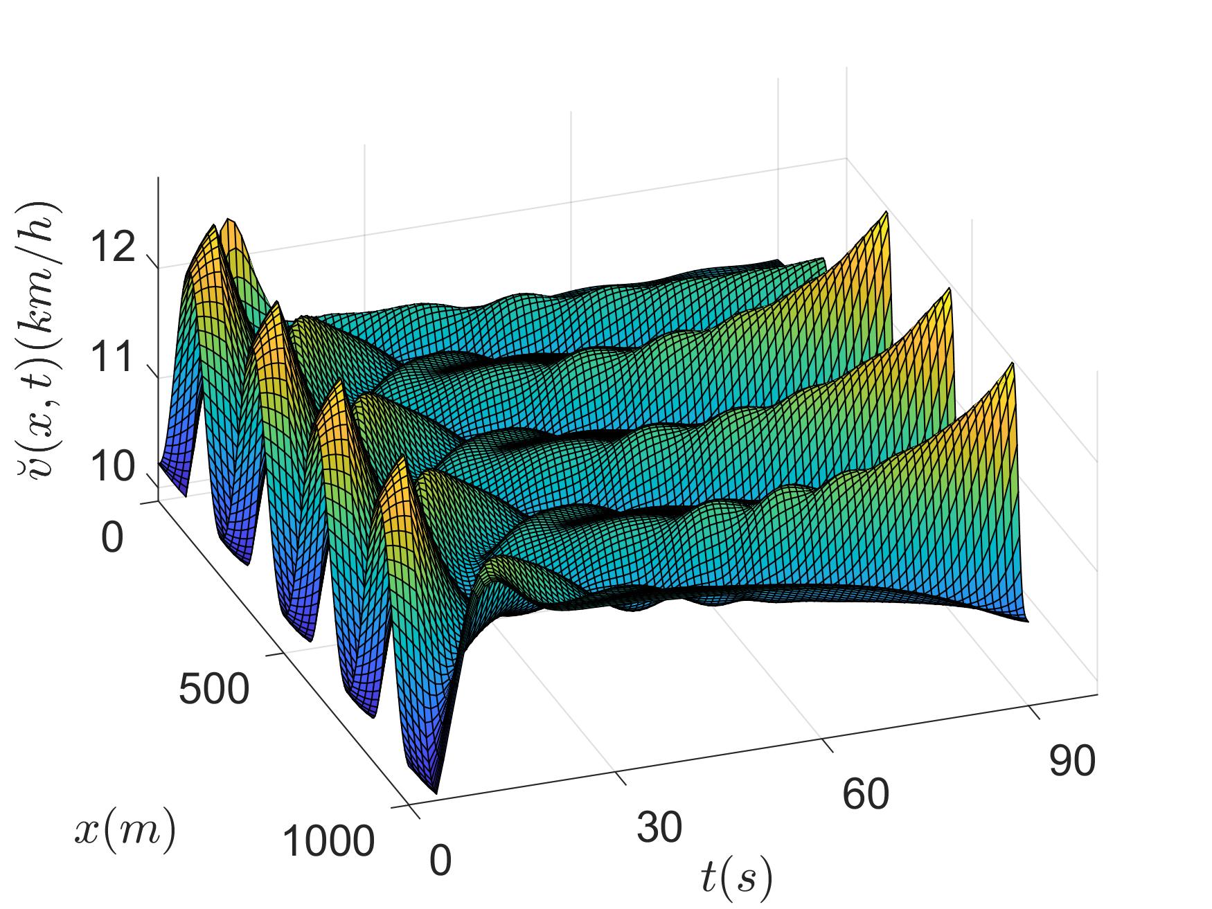
Fig. 5: The evolution of the traffic states and the actuator: (a) $\breve{\rho}(x,t)$ without delay-compensation; (b) $\breve{v}(x,t)$ without delay-compensation; (c) control effort $\breve{h}_{\rm{acc}}(x,t)$ with no delay-compensation; (d) $\breve{\rho}(x,t)$ with delay-compensator; (e) state $\breve{v}(x,t)$ with delay-compensator; (f) control effort $\breve{h}_{\rm{acc}}(x,t)$ with delay-compensator; (g) the $L_{2}$ norm of state $\breve{\rho}(x,t)$ for delay matched and delay mismatched cases; (h) the $L_{2}$ norm of state $\breve{v}(x,t)$ for delay matched and delay mismatched cases; (i) the $L_{2}$ norm of control $\breve{h}_{\rm{acc}}(x,t)$ for delay matched and delay mismatched cases.

Lemma 4.

The Lyapunov functions $V_{1}$ defined in (81) and $V_{2}$ defined in (82) are equivalent in the sense of the $L_{2}$ norm, i.e., there exist positive constants $\alpha_{1}$ and $\alpha_{2}$ , such that

$$\alpha_{1}V_{2}(t)\leq V_{1}(t)\leq\alpha_{2}V_{2}(t).$$ (102)

Since the transformation (64) and the inverse transformation (94) are presented in explicit form and they are bounded, the $L_{2}$ norm equivalence between the Lyapunov functions $V_{1}$ and $V_{2}$ is easily established from Theorem 1.2 [1]. Combining Lemma 2-4, we reach Theorem 1.

V Simulation

In this section, we illustrate our results with an numerical example. We apply the control law (79) directly on the nonlinear model (1)-(4). The parameters utilized in the simulation are shown in Table I, for which we choose the same values as those in [4].

TABLE I: PARAMETERS OF SYSTEM

$L=1000~{}\rm{m}$	$l=5~{}\rm{m}$	$q_{\rm{in}}=1200~{}\rm{veh}/h$
$\tau_{\rm{acc}}=2~{}\rm{s}$	$\tau_{\rm{m}}=60~{}\rm{s}$	$\breve{h}_{\rm{m}}=1~{}\rm{s}$
$\bar{h}_{\rm{acc}}=1.5~{}\rm{s}$	$\breve{\rho}_{\rm{min}}=37\rm{veh}/km$

From (12), we get the value of the mixed steady-state time gap $\bar{h}_{\rm{mix}}=1.35~{}\rm{s}$. The steady-state values for density and speed derived from (11) are $\bar{\rho}=107.36~{}\rm{veh/km}$, $\bar{v}=11.18~{}\rm{km/h}$. The system is discretized with time step $\Delta t=0.5~{}\rm{s}$ and spatial step $\Delta x=5~{}\rm{m}$. The initial conditions are chosen as $\breve{\rho}(x,0)=10\cos(8\pi x/L)$ and $\breve{v}(x,0)=q_{\rm{in}}/\breve{\rho}(x,0)$, which imitates the stop-and-go wave in congested regime. Considering the time delay $D=4~{}{\rm{s}}$ and the coefficient $k=0.1(1/\rm{s})$ of the target system, we first investigate the numerical solution of the nonlinear system (1)-(4) with the non-delay-compensation state-feedback control proposed in [4], whose results are shown in Fig. 5 (a)-(c). It is evident that the response of the system without delay-compensation exhibits an unstable and oscillatory behavior and the stop-and-go wave propagates backward without being attenuated. In contrast, as it is shown in Fig. 5 (d) and (e), the traffic system (1)-(4) is stabilized under the delay-compensator and the oscillations in the speed response are suppressed first and then the oscillations in density response converges to the equilibrium as well. The control effort (79) is shown in Fig. 5 (f), which indicates the resulting values for the time gap of ACC vehicles lie within the interval $[0.8,2.2]~{}\rm{s}$ which is typically implemented in ACC vehicles settings, see, e.g., [21]. In order to illustrate the converging evolution of the states and the actuator more clearly, we plot the states and the control effort in $L_{2}$ norm in solid line, respectively, shown in Fig. 5 (g)-(i), where the dashed line represents the steady-state value.

To examine the robustness of the proposed delay-compensated control law, we conducted some additional simulations with mismatched delays. First, we consider the over-compensation case where the actual delay is less than the delay used in control. The numerical result is shown in Fig. 5 (g)-(i) in dotted line when the actual delay is $3\rm{s}$, while the delay used in control is $4\rm{s}$. Then, we consider the under-compensation case where the actual delay is larger than the delay used in control. The numerical result is also shown in Fig. 5 (g)-(i), where the dash-dotted line represents $L_{2}$ norm of the states $\breve{\rho}$, $\breve{v}$ and the control effort, respectively, when the actual delay is $5\rm{s}$, while the delay used in control is $4\rm{s}$. From the simulation results, we find the closed-loop system remains stable in delay mismatched conditions. The performance improvement of the closed-loop system under the proposed controller (79) is also illustrated in simulation by employing three metrics, namely, total travel time (TTT), fuel consumption and comfort, where we use the same definition as in [30]:

$$J_{\mathrm{TTT}} =\int_{0}^{T}\int_{0}^{L}\rho(x,t)dxdt,$$ (103)

$$J_{\text{fuel }} =\int_{0}^{T}\int_{0}^{L}\xi(x,t)\cdot\rho(x,t)dxdt,$$ (104)

$$J_{\text{comfort }} =\int_{0}^{T}\int_{0}^{L}\left(a(x,t)^{2}+a_{t}(x,t)^{2}\right)\rho(x,t)dxdt,$$ (105)

where we also select the same functions and parameters as those in [30]: $a(x,t)=v_{t}(x,t)+v(x,t)v_{x}(x,t)$, $b_{0}=25\cdot 10^{-3}$, $b_{1}=24.5\cdot 10^{-6}$, $b_{3}=32.5\cdot 10^{-9}$, $b_{4}=125\cdot 10^{-6}$, $\xi(x,t)=\max\left\{0,b_{0}+b_{1}v(x,t)+b_{3}v(x,t)+b_{4}v(x,t)a(x,t)\right\}$ and $T=300~{}\rm{s}$.

TABLE II: PERFORMANCE INDICES

Performance indices	Percentage with improvement
$J_{\mathrm{TTT}}$	$3.91\%$
$J_{\text{fuel }}$	$3.76\%$
$J_{\text{comfort }}$	$92.1\%$

As shown in the Table II, three indicators are improved compared to the open-loop system. Since the open-loop system is unstable, we only consider the first 300 seconds in the simulation. In particular, the driving comfort is significantly improved due to the homogenization of speed which alleviates the phenomenon of stop-and-go oscillation.

VI Conclusion

In this paper, we present a control design methodology for compensation of unstable traffic flow with input delay. The delay is resulting from the time required for the transmission of the control command from the control to the ACC vehicles. Applying the PDE backstepping method, we develop an explicit feedback delay-compensator, composed of the feedback of the traffic speed, the traffic density and the historical actuator states, which is divided into three parts upon the spatial domain along the highway. The closed-loop system, under the developed compensator, was shown to be exponentially stable in the $L_{2}$ sense. Although the control design is based on a linearized system, the numerical simulation shows the effectiveness of the proposed controller on the original nonlinear system. Further research would include delay-robustness and the output feedback control based on observer design.

Appendix A Solving kernel equations

Under Assumption 1, we get the integral equations from (46)–(51) by using the characteristic line method,

$$\gamma(x,s,y)= -\frac{c_{5}}{c_{6}}\mathrm{e}^{-{c}_{2}x}\delta(x-y-c_{1}s)$$

$$-\int_{y}^{y+c_{1}s}\frac{c_{5}}{c_{1}}\mathrm{e}^{-{c}_{2}\theta}\eta(x,\frac{y-\theta}{c_{1}}+s,\theta)d\theta,$$ (106)

$$~{}~{}\mathrm{if}~{}~{}y\leq L-c_{1}s,$$

$$\gamma(x,s,y)= -\int^{s-\frac{L-y}{c_{1}}}_{0}\frac{c_{4}c_{5}}{c_{1}}\mathrm{e}^{-{c}_{2}L}\eta(x,\theta,L)d\theta$$

$$-\int_{y}^{L}\frac{c_{5}}{c_{1}}\mathrm{e}^{-{c}_{2}\theta}\eta(x,\frac{y-\theta}{c_{1}}+s,\theta)d\theta,$$ (107)

$$~{}~{}\mathrm{if}~{}~{}y>L-c_{1}s,$$

$$\eta(x,s,y)= -\frac{c_{1}c_{7}}{c_{4}}\gamma(x,s-\frac{y}{c_{4}},0),$$ (108)

$$~{}~{}\mathrm{if}~{}~{}y\leq c_{4}s,$$

$$\eta(x,s,y)= \frac{k}{c_{6}}\delta(x-(y-c_{4}s)),$$ (109)

$$~{}~{}\mathrm{if}~{}~{}y>c_{4}s.$$

Substitute (108) and (109) into (106) and (107), which gives three-branch expression of $\gamma(x,s,y)$

$$\gamma(x,s,y)= -\int_{0}^{y+c_{1}s}\frac{kc_{5}}{c_{6}(c_{1}+c_{4})}\mathrm{e}^{-\frac{c_{1}c_{2}}{c_{1}+c_{4}}\theta-\frac{c_{2}c_{4}}{c_{1}+c_{4}}(y+c_{1}s)}$$

$$\times\delta(x-\theta)d\theta$$

$$+\int_{0}^{s-\frac{y}{c_{4}}}\frac{c_{1}c_{5}c_{7}}{c_{1}+c_{4}}\mathrm{e}^{\frac{c_{2}c_{4}}{c_{1}+c_{4}}(c_{1}\theta-y-c_{1}s)}\gamma(x,\theta,0)d\theta$$

$$-\frac{c_{5}}{c_{6}}\mathrm{e}^{-{c}_{2}x}\delta(x-y-c_{1}s),$$ (110)

$$~{}~{}\mathrm{if}~{}~{}0\leq y\leq c_{4}s,$$

$$\gamma(x,s,y)= -\int_{y-c_{4}s}^{y+c_{1}s}\frac{kc_{5}}{c_{6}(c_{1}+c_{4})}\mathrm{e}^{-\frac{c_{1}c_{2}}{c_{1}+c_{4}}\theta-\frac{c_{2}c_{4}}{c_{1}+c_{4}}(y+c_{1}s)}$$

$$\times\delta(x-\theta)d\theta$$

$$-\frac{c_{5}}{c_{6}}\mathrm{e}^{-{c}_{2}x}\delta(x-y-c_{1}s),$$ (111)

$$~{}~{}\mathrm{if}~{}~{}c_{4}s<y\leq L-c_{1}s,$$

$$\gamma(x,s,y)= -\int_{y-c_{4}s}^{\frac{c_{1}+c_{4}}{c_{1}}L-\frac{c_{4}}{c_{1}}y-c_{4}s}\frac{kc_{5}}{c_{6}(c_{1}+c_{4})}$$

$$\times\mathrm{e}^{-\frac{c_{1}c_{2}}{c_{1}+c_{4}}\theta-\frac{c_{2}c_{4}}{c_{1}+c_{4}}(y+c_{1}s)}\delta(x-\theta)d\theta$$

$$-\frac{kc_{5}}{c_{1}c_{6}}\mathrm{e}^{-{c}_{2}L},$$ (112)

$$~{}~{}\mathrm{if}~{}~{}L-c_{1}s<y\leq L.$$

We use successive approximations method for (110) and get the following iterations:

$$\gamma^{n+1}(x,s,y)=-\frac{kc_{5}}{c_{6}(c_{1}+c_{4})}\mathrm{e}^{-\frac{c_{1}c_{2}}{c_{1}+c_{4}}x-\frac{c_{2}c_{4}}{c_{1}+c_{4}}(y+c_{1}s)}$$

$$-\frac{c_{5}}{c_{6}}\mathrm{e}^{-{c}_{2}x}\delta(x-y-c_{1}s)$$

$$+\int_{0}^{s-\frac{y}{c_{4}}}\frac{c_{1}c_{5}c_{7}}{c_{1}+c_{4}}\mathrm{e}^{\frac{c_{2}c_{4}}{c_{1}+c_{4}}(c_{1}\theta-y-c_{1}s)}\gamma^{n}(x,\theta,0)d\theta,$$

$$~{}~{}~{}~{}~{}~{}~{}\mathrm{if}~{}~{}~{}0\leq x\leq y+c_{1}s,~{}~{}\mathrm{for}~{}n=0,1,2,...$$ (113)

Let

$$\Delta\gamma^{n}(x,s,y)= \gamma^{n+1}(x,s,y)-\gamma^{n}(x,s,y),$$ (114)

then,

$$\Delta\gamma^{0}(x,s,y)= -\frac{kc_{5}}{c_{6}(c_{1}+c_{4})}\mathrm{e}^{-\frac{c_{1}c_{2}}{c_{1}+c_{4}}x-\frac{c_{2}c_{4}}{c_{1}+c_{4}}(y+c_{1}s)}$$

$$-\frac{c_{5}}{c_{6}}\mathrm{e}^{-{c}_{2}x}\delta(x-y-c_{1}s),$$ (115)

$$\Delta\gamma^{n}(x,s,y)= \int_{\frac{x}{c_{1}}}^{s-\frac{y}{c_{4}}}\frac{c_{1}c_{5}c_{7}}{c_{1}+c_{4}}\mathrm{e}^{\frac{c_{2}c_{4}}{c_{1}+c_{4}}(c_{1}\theta-y-c_{1}s)}$$

$$\times\Delta\gamma^{n-1}(x,\theta,0)d\theta,$$ (116)

After a series of iterations of $\gamma^{n}$, we have

$$\Delta\gamma^{n}=-\frac{c_{5}}{c_{6}}\mathrm{e}^{-\frac{c_{1}c_{2}}{c_{1}+c_{4}}x-\frac{c_{2}c_{4}}{c_{1}+c_{4}}(y+c_{1}s)}\times$$

$$\left[\frac{c_{5}c_{7}(c_{1}c_{5}c_{7}(s-\frac{y}{c_{4}}-\frac{x}{c_{1}}))^{n-1}}{(n-1)!(c_{1}+c_{4})^{n}}-\frac{k(c_{1}c_{5}c_{7}(s-\frac{y}{c_{4}}-\frac{x}{c_{1}}))^{n}}{n!(c_{1}+c_{4})^{n+1}}\right]$$

$$~{}~{}~{}~{}~{}~{}~{}~{}~{}~{}~{}~{}~{}~{}~{}\mathrm{if}~{}~{}0\leq y\leq c_{4}s-\frac{c_{4}}{c_{1}}x,$$ (117)

then,

$$\gamma (x,s,y)=\sum_{n=1}^{+\infty}\Delta\gamma^{n}(x,s,y)+\Delta\gamma^{0}(x,s,y)$$

$$= -\frac{c_{5}(k+c_{5}c_{7})}{c_{6}(c_{1}+c_{4})}\mathrm{e}^{-c_{2}(x+y)}-\frac{c_{5}}{c_{6}}\mathrm{e}^{-{c}_{2}x}\delta(x-y-c_{1}s),$$

$$~{}~{}~{}~{}~{}\mathrm{if}~{}~{}0\leq y\leq c_{4}s-\frac{c_{4}}{c_{1}}x.$$ (118)

After a direct computing from (111) and (112), we reach (52).

Appendix B The Proof of Lemma 1

First, we prove that the transformation is continuous. Substitute $x=c_{1}s$ into the first and the second case of the transformation (64), which gives

$$T_{1}[\psi(t)](c_{1}s,s)+Z_{1}[z(t)](c_{1}s)+Y_{1}[v(t)](c_{1}s)$$

$$= \psi(c_{1}s,s,t)$$

$$-\int_{0}^{s}c_{1}c_{2}\mathrm{e}^{-c_{1}c_{2}\tau}\psi(c_{1}s-c_{1}\tau,s-\tau,t)d\tau$$

$$+\int_{0}^{s}k\psi(c_{1}s+c_{4}\tau,s-\tau,t)d\tau$$

$$-\int_{0}^{s}\int_{c_{1}s-c_{1}\tau}^{c_{1}s+c_{4}\tau}\frac{kc_{1}c_{2}}{c_{1}+c_{4}}\mathrm{e}^{-\frac{c_{1}c_{2}}{c_{1}+c_{4}}(c_{1}s-y+c_{4}\tau)}$$

$$\times\psi(y,s-\tau,t)dyd\tau$$

$$+\int_{0}^{c_{1}s+c_{4}s}\frac{kc_{5}}{c_{6}(c_{1}+c_{4})}\mathrm{e}^{-c_{1}c_{2}s-\frac{c_{2}c_{4}}{c_{1}+c_{4}}y}z(y,t)dy$$

$$-\frac{c_{5}c_{7}}{c_{6}}\mathrm{e}^{-c_{1}c_{2}s}v(0,t)-\frac{k}{c_{6}}v(c_{1}s+c_{4}s,t),$$ (119)

and

$$T_{2}[\psi(t)](c_{1}s,s)+Z_{2}[z(t)](c_{1}s)+Y_{2}[v(t)](c_{1}s)$$

$$= \psi(c_{1}s,s,t)$$

$$-\int_{0}^{s}c_{1}c_{2}\mathrm{e}^{-c_{1}c_{2}\tau}\psi(c_{1}s-c_{1}\tau,s-\tau,t)d\tau$$

$$+\int_{0}^{s}k\psi(c_{1}s+c_{4}\tau,s-\tau,t)d\tau$$

$$-\int_{0}^{s}\int_{c_{1}s-c_{1}\tau}^{c_{1}s+c_{4}\tau}\frac{kc_{1}c_{2}}{c_{1}+c_{4}}\mathrm{e}^{-\frac{c_{1}c_{2}}{c_{1}+c_{4}}(c_{1}s-y+c_{4}\tau)}$$

$$\times\psi(y,s-\tau,t)dyd\tau$$

$$+\frac{c_{5}}{c_{6}}\mathrm{e}^{-c_{1}c_{2}s}z(0,t)$$

$$+\int_{0}^{c_{1}s+c_{4}s}\frac{kc_{5}}{c_{6}(c_{1}+c_{4})}\mathrm{e}^{-c_{1}c_{2}s-\frac{c_{2}c_{4}}{c_{1}+c_{4}}y}z(y,t)dy$$

$$-\frac{k}{c_{6}}v(c_{1}s+c_{4}s,t),$$ (120)

It shows that (B) equals to (B) by using the the boundary condition (26). In a similar way, one can get

$$T_{2}[\psi(t)](L-c_{4}s,s)= T_{3}[\psi(t)](L-c_{4}s,s),$$

$$Z_{2}[z(t)](L-c_{4}s)= Z_{3}[z(t)](L-c_{4}s),$$

$$Y_{2}[v(t)](L-c_{4}s,s)= \frac{k}{c_{6}}v(L,t),$$

which implies the transformation (64) in the second and third case has a same value at $x=L-c_{4}s$.

Second, it is obvious that the transformation is bounded from the explicit form of each kernel function.

Third, differentiating the transformation (64) with respect to $t$ and $s$, respectively, and then substituting them into (36) and (37), one can prove the system (24)-(29) can be transformed into (III-A)-(37) via (64) after a lengthy computation. The details are shown as follows: in the case of $0\leq x<c_{1}s$,

$$\beta_{s}(x,s,t)=\psi_{s}(x,s,t)$$

$$~{}~{}~{}+\frac{c_{4}c_{5}(k+c_{5}c_{7})}{c_{6}(c_{1}+c_{4})}\mathrm{e}^{-c_{2}(c_{4}s+\frac{c_{1}-c_{4}}{c_{1}}x)}z(c_{4}(s-\frac{x}{c_{1}}),t)$$

$$~{}~{}~{}+\frac{kc_{4}c_{5}}{c_{6}(c_{1}+c_{4})}\mathrm{e}^{-c_{2}(x+c_{4}s)}z(x+c_{4}s,t)$$

$$~{}~{}~{}-\frac{kc_{4}c_{5}}{c_{6}(c_{1}+c_{4})}\mathrm{e}^{\frac{c_{2}(c_{4}-c_{1})}{c_{1}}x-c_{2}c_{4}s}z(c_{4}(s-\frac{x}{c_{1}}),t)$$

$$~{}~{}~{}-\int_{c_{4}(s-\frac{x}{c_{1}})}^{x+c_{4}s}\frac{kc_{1}c_{2}c_{4}c_{5}}{c_{6}(c_{1}+c_{4})^{2}}\mathrm{e}^{-\frac{c_{1}c_{2}}{c_{1}+c_{4}}x-\frac{c_{2}c_{4}}{c_{1}+c_{4}}(y+c_{1}s)}$$

$$~{}~{}~{}\times z(y,t)dy$$

$$~{}~{}~{}-\frac{c_{4}c_{5}c_{7}}{c_{6}}\mathrm{e}^{-c_{2}x}v_{x}(c_{4}(s-\frac{x}{c_{1}}),t)$$

$$~{}~{}~{}-\frac{kc_{4}}{c_{6}}v_{x}(x+c_{4}s,t)$$

$$~{}~{}~{}-\frac{c_{1}c_{5}c_{7}(k+c_{5}c_{7})}{c_{6}(c_{1}+c_{4})}\mathrm{e}^{-c_{2}x}v(c_{4}(s-\frac{x}{c_{1}}),t)$$

$$~{}~{}~{}-\int_{0}^{\frac{x}{c_{1}}}c_{1}c_{2}\mathrm{e}^{-c_{1}c_{2}r}\psi_{s}(x-c_{1}r,s-r,t)dr$$

$$~{}~{}~{}+\int_{\frac{x}{c_{1}}}^{s}c_{5}c_{7}\mathrm{e}^{-c_{2}x}\psi_{s}(c_{4}(r-\frac{x}{c_{1}}),s-r,t)dr$$

$$~{}~{}~{}+c_{5}c_{7}\mathrm{e}^{-c_{2}x}\psi(c_{4}(s-\frac{x}{c_{1}}),0,t)$$

$$~{}~{}~{}+\int_{0}^{s}k\psi_{s}(x+c_{4}r,s-r,t)dr$$

$$~{}~{}~{}+k\psi(x+c_{4}s,0,t)$$

$$~{}~{}~{}-\int_{0}^{s}\int_{\max\{x-c_{1}r,c_{4}(r-\frac{x}{c_{1}})\}}^{x+c_{4}r}\frac{kc_{1}c_{2}}{c_{1}+c_{4}}\mathrm{e}^{-\frac{c_{1}c_{2}}{c_{1}+c_{4}}(x-y+c_{4}r)}$$

$$~{}~{}~{}\times\psi_{s}(y,s-r,t)dydr$$

$$~{}~{}~{}-\int_{c_{4}(s-\frac{x}{c_{1}})}^{x+c_{4}s}\frac{kc_{1}c_{2}}{c_{1}+c_{4}}\mathrm{e}^{-\frac{c_{1}c_{2}}{c_{1}+c_{4}}(x-y+c_{4}s)}\psi(y,0,t)dydr;$$ (121)

in the case of $c_{1}s<x\leq L-c_{4}s$,

$$\beta_{s}(x,s,t)=\psi_{s}(x,s,t)$$

$$~{}~{}~{}-\frac{c_{1}c_{5}}{c_{6}}\mathrm{e}^{-c_{2}x}z_{x}(x-c_{1}s,t)$$

$$~{}~{}~{}+\frac{kc_{4}c_{5}}{c_{6}(c_{1}+c_{4})}\mathrm{e}^{-c_{2}(x+c_{4}s)}z(x+c_{4}s,t)$$

$$~{}~{}~{}+\frac{kc_{1}c_{5}}{c_{6}(c_{1}+c_{4})}\mathrm{e}^{-c_{2}x}z(x-c_{1}s,t)$$

$$~{}~{}~{}-\int_{x-c_{1}s}^{x+c_{4}s}\frac{kc_{1}c_{2}c_{4}c_{5}}{c_{6}(c_{1}+c_{4})^{2}}\mathrm{e}^{-\frac{c_{1}c_{2}}{c_{1}+c_{4}}x-\frac{c_{2}c_{4}}{c_{1}+c_{4}}(y+c_{1}s)}z(y,t)dy$$

$$~{}~{}~{}-\frac{kc_{4}}{c_{6}}v_{x}(x+c_{4}s,t)$$

$$~{}~{}~{}-\int_{0}^{s}c_{1}c_{2}\mathrm{e}^{-c_{1}c_{2}r}\psi_{s}(x-c_{1}r,s-r,t)dr$$

$$~{}~{}~{}-c_{1}c_{2}\mathrm{e}^{-c_{1}c_{2}s}\psi(x-c_{1}s,0,t)$$

$$~{}~{}~{}+\int_{0}^{s}k\psi_{s}(x+c_{4}r,s-r,t)dr$$

$$~{}~{}~{}+k\psi(x+c_{4}s,0,t)$$

$$~{}~{}~{}-\int_{0}^{s}\int_{x-c_{1}r}^{x+c_{4}r}\frac{kc_{1}c_{2}}{c_{1}+c_{4}}\mathrm{e}^{-\frac{c_{1}c_{2}}{c_{1}+c_{4}}(x-y+c_{4}r)}$$

$$~{}~{}~{}\times\psi_{s}(y,s-r,t)dydr$$

$$~{}~{}~{}-\int_{x-c_{1}s}^{x+c_{4}s}\frac{kc_{1}c_{2}}{c_{1}+c_{4}}\mathrm{e}^{-\frac{c_{1}c_{2}}{c_{1}+c_{4}}(x-y+c_{4}s)}$$

$$~{}~{}~{}\times\psi(y,0,t)dy;$$ (122)

and in the case of $L-c_{4}s<x\leq L$,

$$\beta_{s}(x,s,t)=\psi_{s}(x,s,t)$$

$$~{}~{}~{}-\frac{c_{1}c_{5}}{c_{6}}\mathrm{e}^{-c_{2}x}z_{x}(x-c_{1}s,t)$$

$$~{}~{}~{}-\frac{kc_{1}c_{5}}{c_{6}(c_{1}+c_{4})}\mathrm{e}^{-c_{2}L}z(\frac{c_{1}+c_{4}}{c_{4}}L-\frac{c_{1}}{c_{4}}x-c_{1}s,t)$$

$$~{}~{}~{}+\frac{kc_{1}c_{5}}{c_{6}(c_{1}+c_{4})}\mathrm{e}^{-c_{2}x}z(x-c_{1}s,t)$$

$$~{}~{}~{}-\int_{x-c_{1}s}^{\frac{c_{1}+c_{4}}{c_{4}}L-\frac{c_{1}}{c_{4}}x-c_{1}s}\frac{kc_{1}c_{2}c_{4}c_{5}}{c_{6}(c_{1}+c_{4})^{2}}$$

$$~{}~{}~{}\times\mathrm{e}^{-\frac{c_{1}c_{2}}{c_{1}+c_{4}}x-\frac{c_{2}c_{4}}{c_{1}+c_{4}}(y+c_{1}s)}z(y,t)dy$$

$$~{}~{}~{}+\frac{kc_{5}}{c_{6}}\mathrm{e}^{c_{2}L}z(\frac{c_{1}+c_{4}}{c_{4}}L-\frac{c_{1}}{c_{4}}x-c_{1}s,t)$$

$$~{}~{}~{}-\int_{0}^{s}c_{1}c_{2}\mathrm{e}^{-c_{1}c_{2}r}\psi_{s}(x-c_{1}r,s-r,t)dr$$

$$~{}~{}~{}-c_{1}c_{2}\mathrm{e}^{-c_{1}c_{2}s}\psi(x-c_{1}s,0,t)$$

$$~{}~{}~{}+\int_{0}^{\frac{L-x}{c_{4}}}k\psi_{s}(x+c_{4}r,s-r,t)dr$$

$$~{}~{}~{}+\int_{\frac{L-x}{c_{4}}}^{s}k\psi_{s}(L,s-r,t)dr$$

$$~{}~{}~{}+k\psi(L,0,t)dr$$

$$~{}~{}~{}-\int_{0}^{s}\int_{x-c_{1}r}^{\min\{x+c_{4}r,\frac{c_{1}+c_{4}}{c_{4}}L-\frac{c_{1}}{c_{4}}x-c_{1}r\}}\frac{kc_{1}c_{2}}{c_{1}+c_{4}}$$

$$~{}~{}~{}\times\mathrm{e}^{-\frac{c_{1}c_{2}}{c_{1}+c_{4}}(x-y+c_{4}r)}\psi_{s}(y,s-r,t)dydr$$

$$~{}~{}~{}-\int_{x-c_{1}s}^{\frac{c_{1}+c_{4}}{c_{4}}L-\frac{c_{1}}{c_{4}}x-c_{1}s}\frac{kc_{1}c_{2}}{c_{1}+c_{4}}$$

$$~{}~{}~{}\times\mathrm{e}^{-\frac{c_{1}c_{2}}{c_{1}+c_{4}}(x-y+c_{4}s)}\psi(y,0,t)dy$$

$$~{}~{}~{}-\int_{\frac{L-x}{c_{4}}}^{s}\int_{\frac{c_{1}+c_{4}}{c_{4}}L-\frac{c_{1}}{c_{4}}x-c_{1}r}^{L}kc_{2}\mathrm{e}^{-c_{2}L}\psi_{s}(y,s-r,t)dydr$$

$$~{}~{}~{}-\int_{\frac{c_{1}+c_{4}}{c_{4}}L-\frac{c_{1}}{c_{4}}x-c_{1}s}^{L}kc_{2}\mathrm{e}^{-c_{2}L}\psi(y,0,t)dy.$$ (123)

Then, differentiating (64) with respect of $t$, substituting (24), (25), (27) and (28) to the time derivative of (64), and using integration by parts, we have $\beta_{t}$ in three cases as follows: in the case of $0\leq x<c_{1}s$,

$$\beta_{t}(x,s,t)=\psi_{t}(x,s,t)$$

$$~{}~{}~{}-\frac{c_{1}c_{5}(k+c_{5}c_{7})}{c_{6}(c_{1}+c_{4})}\mathrm{e}^{-c_{2}(c_{4}s+\frac{c_{1}-c_{4}}{c_{1}}x)}z(c_{4}(s-\frac{x}{c_{1}}),t)$$

$$~{}~{}~{}+\frac{c_{1}c_{5}(k+c_{5}c_{7})}{c_{6}(c_{1}+c_{4})}\mathrm{e}^{-c_{2}x}z(0,t)$$

$$~{}~{}~{}-\int_{0}^{c_{4}(s-\frac{x}{c_{1}})}\frac{c_{1}c_{2}c_{5}(k+c_{5}c_{7})}{c_{6}(c_{1}+c_{4})}\mathrm{e}^{-c_{2}(x+y)}z(y,t)dy$$

$$~{}~{}~{}-\int_{0}^{c_{4}(s-\frac{x}{c_{1}})}\frac{c_{1}c_{2}(k+c_{5}c_{7})}{c_{1}+c_{4}}\mathrm{e}^{-c_{2}x}\psi(y,0,t)dy$$

$$~{}~{}~{}-\frac{kc_{1}c_{5}}{c_{6}(c_{1}+c_{4})}\mathrm{e}^{-c_{2}(x+c_{4}s)}z(x+c_{4}s,t)$$

$$~{}~{}~{}+\frac{kc_{1}c_{5}}{c_{6}(c_{1}+c_{4})}\mathrm{e}^{\frac{c_{2}(c_{4}-c_{1})}{c_{1}}x-c_{2}c_{4}s}z(c_{4}(s-\frac{x}{c_{1}}),t)$$

$$~{}~{}~{}-\int_{c_{4}(s-\frac{x}{c_{1}})}^{x+c_{4}s}\frac{kc_{1}c_{2}c_{4}c_{5}}{c_{6}(c_{1}+c_{4})^{2}}\mathrm{e}^{-\frac{c_{1}c_{2}}{c_{1}+c_{4}}x-\frac{c_{2}c_{4}}{c_{1}+c_{4}}(y+c_{1}s)}$$

$$~{}~{}~{}\times z(y,t)dy$$

$$~{}~{}~{}-\int_{c_{4}(s-\frac{x}{c_{1}})}^{x+c_{4}s}\frac{kc_{1}c_{2}}{c_{1}+c_{4}}\mathrm{e}^{-\frac{c_{1}c_{2}}{c_{1}+c_{4}}(x-y+c_{4}s)}$$

$$~{}~{}~{}\times\psi(y,0,t)dy$$

$$~{}~{}~{}-\frac{c_{4}c_{5}c_{7}}{c_{6}}\mathrm{e}^{-c_{2}x}v_{x}(c_{4}(s-\frac{x}{c_{1}}),t)$$

$$~{}~{}~{}+\frac{c_{5}^{2}c_{7}}{c_{6}}\mathrm{e}^{-c_{2}(c_{4}s+\frac{c_{1}-c_{4}}{c_{1}}x)}z(c_{4}(s-\frac{x}{c_{1}}),t)$$

$$~{}~{}~{}+c_{5}c_{7}\mathrm{e}^{-c_{2}x}\psi(c_{4}(s-\frac{x}{c_{1}}),0,t)$$

$$~{}~{}~{}-\frac{kc_{4}}{c_{6}}v_{x}(x+c_{4}s,t)$$

$$~{}~{}~{}+\frac{kc_{5}}{c_{6}}\mathrm{e}^{-c_{2}(x+c_{4}s)}z(x+c_{4}s,t)$$

$$~{}~{}~{}+k\psi(x+c_{4}s,0,t)$$

$$~{}~{}~{}-\frac{c_{1}c_{5}c_{7}(k+c_{5}c_{7})}{c_{6}(c_{1}+c_{4})}\mathrm{e}^{-c_{2}x}v(c_{4}(s-\frac{x}{c_{1}}),t)$$

$$~{}~{}~{}+\frac{c_{1}c_{5}c_{7}(k+c_{5}c_{7})}{c_{6}(c_{1}+c_{4})}\mathrm{e}^{-c_{2}x}v(0,t)$$

$$~{}~{}~{}+\int_{0}^{c_{4}(s-\frac{x}{c_{1}})}\frac{c_{1}c_{2}c_{5}(k+c_{5}c_{7})}{c_{6}(c_{1}+c_{4})}\mathrm{e}^{-c_{2}(x+y)}z(y,t)dy$$

$$~{}~{}~{}+\int_{0}^{c_{4}(s-\frac{x}{c_{1}})}\frac{c_{1}c_{5}c_{7}(k+c_{5}c_{7})}{c_{4}(c_{1}+c_{4})}\mathrm{e}^{-c_{2}x}\psi(y,0,t)dy$$

$$~{}~{}~{}-\int_{0}^{\frac{x}{c_{1}}}c_{1}c_{2}\mathrm{e}^{-c_{1}c_{2}r}\psi_{t}(x-c_{1}r,s-r,t)dr$$

$$~{}~{}~{}+\int_{\frac{x}{c_{1}}}^{s}c_{5}c_{7}\mathrm{e}^{-c_{2}x}\psi_{t}(c_{4}(r-\frac{x}{c_{1}}),s-r,t)dr$$

$$~{}~{}~{}+\int_{0}^{s}k\psi_{t}(x+c_{4}r,s-r,t)dr$$

$$~{}~{}~{}-\int_{0}^{s}\int_{\max\{x-c_{1}r,c_{4}(r-\frac{x}{c_{1}})\}}^{x+c_{4}r}\frac{kc_{1}c_{2}}{c_{1}+c_{4}}\mathrm{e}^{-\frac{c_{1}c_{2}}{c_{1}+c_{4}}(x-y+c_{4}r)}$$

$$~{}~{}~{}\times\psi_{t}(y,s-r,t)dydr;$$ (124)

in the case of $c_{1}s<x\leq L-c_{4}s$,

$$\beta_{t}(x,s,t)=\psi_{t}(x,s,t)$$

$$~{}~{}~{}-\frac{c_{1}c_{5}}{c_{6}}\mathrm{e}^{-c_{2}x}z_{x}(x-c_{1}s,t)$$

$$~{}~{}~{}-c_{1}c_{2}\mathrm{e}^{-c_{1}c_{2}s}\psi(x-c_{1}s,0,t)$$

$$~{}~{}~{}-\frac{kc_{1}c_{5}}{c_{6}(c_{1}+c_{4})}\mathrm{e}^{-c_{2}(x+c_{4}s)}z(x+c_{4}s,t)$$

$$~{}~{}~{}+\frac{kc_{1}c_{5}}{c_{6}(c_{1}+c_{4})}\mathrm{e}^{-c_{2}x}z(x-c_{1}s,t)$$

$$~{}~{}~{}-\int_{x-c_{1}s}^{x+c_{4}s}\frac{kc_{1}c_{2}c_{4}c_{5}}{c_{6}(c_{1}+c_{4})^{2}}\mathrm{e}^{-\frac{c_{1}c_{2}}{c_{1}+c_{4}}x-\frac{c_{2}c_{4}}{c_{1}+c_{4}}(y+c_{1}s)}z(y,t)dy$$

$$~{}~{}~{}-\int_{x-c_{1}s}^{x+c_{4}s}\frac{kc_{1}c_{2}}{c_{1}+c_{4}}\mathrm{e}^{-\frac{c_{1}c_{2}}{c_{1}+c_{4}}(x-y+c_{4}s)}$$

$$~{}~{}~{}\times\psi(y,0,t)dy$$

$$~{}~{}~{}-\frac{kc_{4}}{c_{6}}v_{x}(x+c_{4}s,t)$$

$$~{}~{}~{}+\frac{kc_{5}}{c_{6}}\mathrm{e}^{-c_{2}(x+c_{4}s)}z(x+c_{4}s,t)$$

$$~{}~{}~{}+k\psi(x+c_{4}s,0,t)$$

$$~{}~{}~{}-\int_{0}^{s}c_{1}c_{2}\mathrm{e}^{-c_{1}c_{2}r}\psi_{t}(x-c_{1}r,s-r,t)dr$$

$$~{}~{}~{}+\int_{0}^{s}k\psi_{t}(x+c_{4}r,s-r,t)dr$$

$$~{}~{}~{}-\int_{0}^{s}\int_{x-c_{1}r}^{x+c_{4}r}\frac{kc_{1}c_{2}}{c_{1}+c_{4}}\mathrm{e}^{-\frac{c_{1}c_{2}}{c_{1}+c_{4}}(x-y+c_{4}r)}$$

$$~{}~{}~{}\times\psi_{t}(y,s-r,t)dydr;$$ (125)

in the case of $L-c_{4}s<x\leq L$,

$$\beta_{t}(x,s,t)=\psi_{t}(x,s,t)$$

$$~{}~{}~{}-\frac{c_{1}c_{5}}{c_{6}}\mathrm{e}^{-c_{2}x}z_{x}(x-c_{1}s,t)$$

$$~{}~{}~{}-c_{1}c_{2}\mathrm{e}^{-c_{1}c_{2}s}\psi(x-c_{1}s,0,t)$$

$$~{}~{}~{}-\frac{kc_{1}c_{5}}{c_{6}(c_{1}+c_{4})}\mathrm{e}^{-c_{2}L}z(\frac{c_{1}+c_{4}}{c_{4}}L-\frac{c_{1}}{c_{4}}x-c_{1}s,t)$$

$$~{}~{}~{}+\frac{kc_{1}c_{5}}{c_{6}(c_{1}+c_{4})}\mathrm{e}^{-c_{2}x}z(x-c_{1}s,t)$$

$$~{}~{}~{}-\int_{x-c_{1}s}^{\frac{c_{1}+c_{4}}{c_{4}}L-\frac{c_{1}}{c_{4}}x-c_{1}s}\frac{kc_{1}c_{2}c_{4}c_{5}}{c_{6}(c_{1}+c_{4})^{2}}$$

$$~{}~{}~{}\times\mathrm{e}^{-\frac{c_{1}c_{2}}{c_{1}+c_{4}}x-\frac{c_{2}c_{4}}{c_{1}+c_{4}}(y+c_{1}s)}z(y,t)dy$$

$$~{}~{}~{}-\int_{x-c_{1}s}^{\frac{c_{1}+c_{4}}{c_{4}}L-\frac{c_{1}}{c_{4}}x-c_{1}s}\frac{kc_{1}c_{2}}{c_{1}+c_{4}}$$

$$~{}~{}~{}\times\mathrm{e}^{-\frac{c_{1}c_{2}}{c_{1}+c_{4}}(x-y+c_{4}s)}\psi(y,0,t)dy$$

$$~{}~{}~{}-\frac{kc_{5}}{c_{6}}\mathrm{e}^{c_{2}L}z(L,t)$$

$$~{}~{}~{}+\frac{kc_{5}}{c_{6}}\mathrm{e}^{c_{2}L}z(\frac{c_{1}+c_{4}}{c_{4}}L-\frac{c_{1}}{c_{4}}x-c_{1}s,t)$$

$$~{}~{}~{}-\int_{\frac{c_{1}+c_{4}}{c_{4}}L-\frac{c_{1}}{c_{4}}x-c_{1}s}^{L}kc_{2}\mathrm{e}^{-c_{2}L}\psi(y,0,t)dy$$

$$~{}~{}~{}+\frac{kc_{5}}{c_{6}}\mathrm{e}^{c_{2}L}z(L,t)$$

$$~{}~{}~{}+k\psi(L,0,t)dr$$

$$~{}~{}~{}-\int_{0}^{s}c_{1}c_{2}\mathrm{e}^{-c_{1}c_{2}r}\psi_{t}(x-c_{1}r,s-r,t)dr$$

$$~{}~{}~{}+\int_{0}^{\frac{L-x}{c_{4}}}k\psi_{t}(x+c_{4}r,s-r,t)dr$$

$$~{}~{}~{}+\int_{\frac{L-x}{c_{4}}}^{s}k\psi_{t}(L,s-r,t)dr$$

$$~{}~{}~{}-\int_{0}^{s}\int_{x-c_{1}r}^{\min\{x+c_{4}r,\frac{c_{1}+c_{4}}{c_{4}}L-\frac{c_{1}}{c_{4}}x-c_{1}r\}}\frac{kc_{1}c_{2}}{c_{1}+c_{4}}$$

$$~{}~{}~{}\times\mathrm{e}^{-\frac{c_{1}c_{2}}{c_{1}+c_{4}}(x-y+c_{4}r)}\psi_{t}(y,s-r,t)dydr$$

$$~{}~{}~{}-\int_{\frac{L-x}{c_{4}}}^{s}\int_{\frac{c_{1}+c_{4}}{c_{4}}L-\frac{c_{1}}{c_{4}}x-c_{1}r}^{L}kc_{2}\mathrm{e}^{-c_{2}L}\psi_{t}(y,s-r,t)dydr.$$ (126)

For each case, one can reach $\beta_{t}(x,s,t)-\beta_{s}(x,s,t)=0$. In order to get (III-A), (33) and (35) of the target system, we get the relation between $\psi$ and $\beta$ at $s=0$ via transformation (64) as follows:

$$\psi(x,0,t)=\beta(x,0,t)-\frac{c_{5}}{c_{6}}\mathrm{e}^{-c_{2}x}z(x,t)+\frac{k}{c_{6}}v(x,t).$$ (127)

Substitute (127) into (24), (25) and (27), respectively, which gives (III-A), (33) and (35). Hence, the transformation (64) can transform the original system (24)-(29) into the target system (III-A)-(37).

Jie Qi is Professor of Automation Department at the Donghua University, China. She received her Ph.D. degree in Systems Engineering (2005) and the B.S. degree in Automation (2000) from Northeastern University in Shenyang, China. She has been a research fellow with the Institute of Textiles & Clothing, the Hong Kong Polytechnic University, Hong Kong from 2007 to 2008; a visiting researcher with the Cymer Center for Control Systems and Dynamics at the University of California, San Diego, from March 2013 to February 2014 and from June to September in 2015; and a visiting researcher with the Chemical and Materials Engineering Department at the University of Alberta, from January 2019 to January 2020. Her research interests include control and estimation of distributed parameters systems, control of delayed systems and its applications on multi-agent systems and traffic systems.

Shurong Mo received his B.S. degree in Automation from Donghua University in 2018. He participated in the National Undergraduate Electronic Design Contest and won the third prize, in 2017. He is currently pursuing his M.S. degree in Control Science and Control Engineering at Donghua University. His research interests include control of delayed systems, reinforcement learning-based control of traffic systems.

Miroslav Krstic is Distinguished Professor of Mechanical and Aerospace Engineering, holds the Alspach endowed chair, and is the founding director of the Cymer Center for Control Systems and Dynamics at UC San Diego. He also serves as Senior Associate Vice Chancellor for Research at UCSD. As a graduate student, Krstic won the UC Santa Barbara best dissertation award and student best paper awards at CDC and ACC. Krstic has been elected Fellow of seven scientific societies - IEEE, IFAC, ASME, SIAM, AAAS, IET (UK), and AIAA (Assoc. Fellow) - and as a foreign member of the Serbian Academy of Sciences and Arts and of the Academy of Engineering of Serbia. He has received the Richard E. Bellman Control Heritage Award, SIAM Reid Prize, ASME Oldenburger Medal, Nyquist Lecture Prize, Paynter Outstanding Investigator Award, Ragazzini Education Award, IFAC Nonlinear Control Systems Award, Chestnut textbook prize, Control Systems Society Distinguished Member Award, the PECASE, NSF Career, and ONR Young Investigator awards, the Schuck (’96 and ’19) and Axelby paper prizes, and the first UCSD Research Award given to an engineer. Krstic has also been awarded the Springer Visiting Professorship at UC Berkeley, the Distinguished Visiting Fellowship of the Royal Academy of Engineering, the Invitation Fellowship of the Japan Society for the Promotion of Science, and four honorary professorships outside of the United States. He serves as Editor-in-Chief of Systems & Control Letters and has been serving as Senior Editor in Automatica and IEEE Transactions on Automatic Control, as editor of two Springer book series, and has served as Vice President for Technical Activities of the IEEE Control Systems Society and as chair of the IEEE CSS Fellow Committee. Krstic has coauthored fifteen books on adaptive, nonlinear, and stochastic control, extremum seeking, control of PDE systems including turbulent flows, and control of delay systems.

References

• [1] H. Anfinsen and O. Aamo. Adaptive control of hyperbolic PDEs. Springer, 2019.
• [2] J. Auriol, U. J. F. Aarsnes, P. Martin, and F. Di Meglio. Delay-robust control design for two heterodirectional linear coupled hyperbolic PDEs. IEEE Transactions on Automatic Control, 63(10):3551–3557, 2018.
• [3] A. Aw and M. Rascle. Resurrection of ”second order” models of traffic flow. SIAM journal on applied mathematics, 60(3):916–938, 2000.
• [4] N. Bekiaris-Liberis and A. I. Delis. PDE-based feedback control of freeway traffic flow via time-gap manipulation of ACC-equipped vehicles. IEEE Transactions on Control Systems Technology, 29(1):461–469, 2021.
• [5] N. Bekiaris-Liberis, C. Roncoli, and M. Papageorgiou. Highway traffic state estimation per lane in the presence of connected vehicles. Transportation research part B: methodological, 106:1–28, 2017.
• [6] Nikolaos Bekiaris-Liberis and Miroslav Krstic. Compensation of actuator dynamics governed by quasilinear hyperbolic pdes. Automatica, 92:29–40, 2018.
• [7] M. Burger, S. Göttlich, and T. Jung. Derivation of second order traffic flow models with time delays. Networks & Heterogeneous Media, 14(2):265, 2019.
• [8] C. Chen, Z. Jia, and P. Varaiya. Causes and cures of highway congestion. IEEE Control Systems Magazine, 21(6):26–32, 2001.
• [9] S. Darbha and K. Rajagopal. Intelligent cruise control systems and traffic flow stability. Transportation Research Part C: Emerging Technologies, 7(6):329–352, 1999.
• [10] A. I. Delis, I. K. Nikolos, and M. Papageorgiou. Macroscopic traffic flow modeling with adaptive cruise control: Development and numerical solution. Computers & Mathematics with Applications, 70(8):1921–1947, 2015.
• [11] M. Laura Delle Monache, B. Piccoli, and F. Rossi. Traffic regulation via controlled speed limit. SIAM Journal on Control and Optimization, 55(5):2936–2958, 2017.
• [12] C. Diakaki, M. Papageorgiou, I. Papamichail, and I. Nikolos. Overview and analysis of vehicle automation and communication systems from a motorway traffic management perspective. Transportation Research Part A: Policy and Practice, 75:147–165, 2015.
• [13] M. Fountoulakis, N. Bekiaris-Liberis, C. Roncoli, I. Papamichail, and M. Papageorgiou. Highway traffic state estimation with mixed connected and conventional vehicles: Microscopic simulation-based testing. Transportation Research Part C: Emerging Technologies, 78:13–33, 2017.
• [14] T. Hashimoto and M. Krstic. Stabilization of reaction diffusion equations with state delay using boundary control input. IEEE Transactions on Automatic Control, 61(12):4041–4047, 2016.
• [15] I. G. Jin and G. Orosz. Dynamics of connected vehicle systems with delayed acceleration feedback. Transportation Research Part C: Emerging Technologies, 46:46–64, 2014.
• [16] I. Karafyllis, N. Bekiaris-Liberis, and M. Papageorgiou. Feedback control of nonlinear hyperbolic PDE systems inspired by traffic flow models. IEEE Transactions on Automatic Control, 64(9):3647–3662, 2019.
• [17] O. Kolb, S. Göttlich, and P. Goatin. Capacity drop and traffic control for a second order traffic model. Networks & Heterogeneous Media, 12(4):663, 2017.
• [18] M. Krstic. Control of an unstable reaction-diffusion PDE with long input delay. Systems & Control Letters, 58(10-11):773–782, 2009.
• [19] H. Lhachemi, C. Prieur, and R. Shorten. Robustness of constant-delay predictor feedback for in-domain stabilization of reaction–diffusion PDEs with time-and spatially-varying input delays. Automatica, 123:109347, 2021.
• [20] D. Ngoduy. Instability of cooperative adaptive cruise control traffic flow: A macroscopic approach. Communications in Nonlinear Science and Numerical Simulation, 18(10):2838–2851, 2013.
• [21] C. Nowakowski, S. E. Shladover, D. Cody, F. Bu, J. O’Connell, J. Spring, S. Dickey, and D. Nelson. Cooperative adaptive cruise control: Testing drivers’ choices of following distances. Technical report, 2011.
• [22] C. Prieur and E. Trélat. Feedback stabilization of a 1-d linear reaction–diffusion equation with delay boundary control. IEEE Transactions on Automatic Control, 64(4):1415–1425, 2019.
• [23] J. Qi, S. Dubljevic, and W. Kong. Output feedback compensation to state and measurement delays for a first-order hyperbolic PIDE with recycle. Automatica, 128:109565, 2021.
• [24] J. Qi, M. Krstic, and S. Wang. Stabilization of reaction-diffusions PDE with delayed distributed actuation. Systems & Control Letters, 133:104558, 2019.
• [25] J. Qi, S. Wang, J. Fang, and M. Diagne. Control of multi-agent systems with input delay via PDE-based method. Automatica, 106:91–100, 2019.
• [26] H. Sano and M. Wakaiki. Boundary stabilization of first-order hyperbolic equations with input delay. Japan Journal of Industrial and Applied Mathematics, 36(2):325–355, 2019.
• [27] A. Selivanov and E. Fridman. Delayed point control of a reaction-diffusion PDE under discrete-time point measurements. Automatica, 96:224–233, 2018.
• [28] A. Selivanov and E. Fridman. Delayed Hsubscript𝐻{H}_{\infty} control of 2D diffusion systems under delayed pointlike measurements. Automatica, 109:108541, 2019.
• [29] R. E. Stern, S. Cui, Maria L. Delle M., R. Bhadani, M. Bunting, M. Churchill, N. Hamilton, H. Pohlmann, F. Wu, B. Piccoli, et al. Dissipation of stop-and-go waves via control of autonomous vehicles: Field experiments. Transportation Research Part C: Emerging Technologies, 89:205–221, 2018.
• [30] M. Treiber and A. Kesting. Traffic Flow Dynamics-Data, Models and Simulation. Berlin, Germany:Springer, 2013.
• [31] J. Yi and R. Horowitz. Macroscopic traffic flow propagation stability for adaptive cruise controlled vehicles. Transportation Research Part C: Emerging Technologies, 14(2):81–95, 2006.
• [32] H. Yu, M. Diagne, L. Zhang, and M. Krstic. Bilateral boundary control of moving shockwave in lwr model of congested traffic. IEEE Transactions on Automatic Control, 66(3):1429–1436, 2021.
• [33] H. Yu, S. Koga, and M. Krstic. Stabilization of traffic flow with a leading autonomous vehicle. In Dynamic Systems and Control Conference, volume 51906, page V002T22A006. American Society of Mechanical Engineers, 2018.
• [34] H. Yu and M. Krstic. Traffic congestion control on two-lane Aw-Rascle-Zhang model. In 2018 IEEE Conference on Decision and Control (CDC), pages 2144–2149. IEEE, 2018.
• [35] H. Yu and M. Krstic. Traffic congestion control for Aw-Rascle-Zhang model. Automatica, 100:38–51, 2019.
• [36] H. M. Zhang. A non-equilibrium traffic model devoid of gas-like behavior. Transportation Research Part B: Methodological, 36(3):275–290, 2002.
• [37] L. Zhang and C. Prieur. Necessary and sufficient conditions on the exponential stability of positive hyperbolic systems. IEEE Transactions on Automatic Control, 62(7):3610–3617, 2017.
• [38] L. Zhang, C. Prieur, and J. Qiao. PI boundary control of linear hyperbolic balance laws with stabilization of ARZ traffic flow models. Systems & Control Letters, 123:85–91, 2019.
[Uncaptioned image] Jie Qi is Professor of Automation Department at the Donghua University, China. She received her Ph.D. degree in Systems Engineering (2005) and the B.S. degree in Automation (2000) from Northeastern University in Shenyang, China. She has been a research fellow with the Institute of Textiles & Clothing, the Hong Kong Polytechnic University, Hong Kong from 2007 to 2008; a visiting researcher with the Cymer Center for Control Systems and Dynamics at the University of California, San Diego, from March 2013 to February 2014 and from June to September in 2015; and a visiting researcher with the Chemical and Materials Engineering Department at the University of Alberta, from January 2019 to January 2020. Her research interests include control and estimation of distributed parameters systems, control of delayed systems and its applications on multi-agent systems and traffic systems.
[Uncaptioned image] Shurong Mo received his B.S. degree in Automation from Donghua University in 2018. He participated in the National Undergraduate Electronic Design Contest and won the third prize, in 2017. He is currently pursuing his M.S. degree in Control Science and Control Engineering at Donghua University. His research interests include control of delayed systems, reinforcement learning-based control of traffic systems.
[Uncaptioned image] Miroslav Krstic is Distinguished Professor of Mechanical and Aerospace Engineering, holds the Alspach endowed chair, and is the founding director of the Cymer Center for Control Systems and Dynamics at UC San Diego. He also serves as Senior Associate Vice Chancellor for Research at UCSD. As a graduate student, Krstic won the UC Santa Barbara best dissertation award and student best paper awards at CDC and ACC. Krstic has been elected Fellow of seven scientific societies - IEEE, IFAC, ASME, SIAM, AAAS, IET (UK), and AIAA (Assoc. Fellow) - and as a foreign member of the Serbian Academy of Sciences and Arts and of the Academy of Engineering of Serbia. He has received the Richard E. Bellman Control Heritage Award, SIAM Reid Prize, ASME Oldenburger Medal, Nyquist Lecture Prize, Paynter Outstanding Investigator Award, Ragazzini Education Award, IFAC Nonlinear Control Systems Award, Chestnut textbook prize, Control Systems Society Distinguished Member Award, the PECASE, NSF Career, and ONR Young Investigator awards, the Schuck (’96 and ’19) and Axelby paper prizes, and the first UCSD Research Award given to an engineer. Krstic has also been awarded the Springer Visiting Professorship at UC Berkeley, the Distinguished Visiting Fellowship of the Royal Academy of Engineering, the Invitation Fellowship of the Japan Society for the Promotion of Science, and four honorary professorships outside of the United States. He serves as Editor-in-Chief of Systems & Control Letters and has been serving as Senior Editor in Automatica and IEEE Transactions on Automatic Control, as editor of two Springer book series, and has served as Vice President for Technical Activities of the IEEE Control Systems Society and as chair of the IEEE CSS Fellow Committee. Krstic has coauthored fifteen books on adaptive, nonlinear, and stochastic control, extremum seeking, control of PDE systems including turbulent flows, and control of delay systems.