Non-Hermitian non-Abelian topological insulators with $PT$ symmetry

Abstract

We study a non-Hermitian non-Abelian topological insulator preserving $PT$ symmetry, where the non-Hermitian term represents nonreciprocal hoppings. As it increases, a spontaneous $PT$ symmetry breaking transition occurs in the perfect-flat band model from a real-line-gap topological insulator into an imaginary-line-gap topological insulator. By introducing a band bending term, we realize two phase transitions, where a metallic phase emerges between the above two topological insulator phases. We discuss an electric-circuit realization of non-Hermitian non-Abelian topological insulators. We find that the spontaneous $PT$ symmetry breaking as well as the edge states are well observed by the impedance resonance.

I Introduction

Topological insulators are one of the most fascinating ideas in contemporary physicsHasan ; Qi . They are characterized by topological numbers such as the winding number, the Chern number and the $\mathbb{Z}_{2}$ index. However, all of these topological numbers are Abelian.

Non-Abelian topological charges are discussed in three-band models protected by $PT$ symmetryWuScience ; Tiwari ; Guo ; YangPRL ; Leng or $C_{2}T$ symmetryBouhon ; DWang . They are realized in nodal line semimetalsWuScience ; Tiwari ; YangPRL ; Leng ; MWang ; BJiang ; HPark in three dimensions and Weyl pointsBouhon in two dimensions. Non-Abelian topological insulators in one dimension are studied for three-band modelsGuo and four-band modelsJiang4 . They are experimentally observed in photonic systemsYangPRL ; DWang , phononic systemsBJiang ; BPeng and transmission linesGuo ; Jiang4 . In addition, a generalization to multi-band theories is proposed in nodal line semimetalsWuScience . As far as we aware of, there is no study on non-Hermitian non-Abelian topological phases so far.

Non-Hermitian topological physics have attracted much attentionBender ; Bender2 ; Malzard ; Konotop ; Rako ; Gana ; Zhu ; Yao ; Jin ; Liang ; Nori ; Lieu ; UedaPRX ; Coba ; Jiang ; JPhys ; Ashida . In non-Hermitian systems eigenvalues and eigenfunctions are complex in general. However, they are restricted to be real if $PT$ symmetry is imposedBender ; Mosta ; Ruter ; Yuce ; LFeng ; Gana ; Weimann . There is a $PT$ symmetry breaking transition, where the eigenvalues and eigenfunctions become complex. Nonreciprocal hopping is such a hopping that the right-going and left-going hopping amplitude are differentHatano . It makes a system non-Hermitian.

In this paper, we study a non-Hermitian non-Abelian topological insulator in an $N$ band model with $PT$ symmetry. We show that a spontaneous $PT$ symmetry breaking is induced by increasing the nonreciprocal hoppings from a phase transition from a real-line-gap topological insulator to an imaginary-line-gap topological insulator in the case of a perfect-flat band model. Furthermore, by introducing a band bending term, we may generalize the model to have a metal with two critical points, where a metallic phase emerges between the above two topological insulator phases. Finally, we show how to implement the present model in electric circuits. The edge states and the spontaneous $PT$ symmetry breaking are well signaled by the impedance resonance.

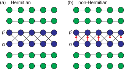
Figure 1: Illustration of the tight-binding Hamiltonian. (a) Hermitian and (b) non-Hermitian models. Interactions between the $\alpha$ and $\beta$ chains yield a non-Abelian topological number. All other chains shown in green act as spectators. Red arrows represent nonreciprocal hoppings.

II Non-Hermitian Non-Abelian topological insulators

II.1 Hermitian Hamiltonian

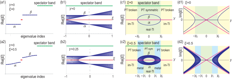
Figure 2: Energy spectrum of the non-Hermitian Hamiltonian in nanoribbon geometry. Eigenvalues of (a1) the perfectly flat $\alpha$ and $\beta$ bands with $\xi=0$ and (a2) the bended bands with $\xi=0.5$ shown in blue. The red dots represent the topological edge states. The band structure as a function of $\xi$ with (b1) $\gamma=0$ and (b2) $\gamma=0.25$. The red lines represent the topological edge states. (c1) and (c2) Real part of the energy. (d1) and (d2) Imaginary part of the energy. We have set $\xi=0$ for (c1) and (d1), while we have set $\xi=0.5$ for (c2) and (d2). The bulk bands are colored in blue, while the edge states are colored in red. The spectator band is colored in green. When $\xi=0$, there are two phases, a real-line-gap topological insulator (real-TI) phase and an imaginary-line-gap topological insulator (im-TI) phase. When $\xi\not=0$, a metallic phase emerges between these two topological insulator phases. We have set $\varepsilon_{\alpha}=1$ and $\varepsilon_{\beta}=2$.

We start with a Hermitian system capable to describe a non-Abelian topological insulator based of the one-dimensional lattice in Fig.1(a). We consider generators of $\mathfrak{so}\left(N\right)$ rotation $L_{\alpha\beta}$ indexed by $\alpha$ and $\beta$, whose $ab$ components are defined by

$$\left(L_{\alpha\beta}\right)_{ab}=\delta_{\alpha b}\delta_{\beta a}-\delta_{\alpha a}\delta_{\beta b}.$$ (1)

We consider a $PT$-invariant Hamiltonian in the momentum space given byWuScience

$$H_{\alpha\beta}\left(k\right)=R_{\alpha\beta}\left(\frac{k}{2}\right)\text{diag.}\left(\varepsilon_{1},\varepsilon_{2},\cdots,\varepsilon_{N}\right)R_{\alpha\beta}\left(\frac{k}{2}\right)^{\text{t}},$$ (2)

where $0\leq k<2\pi$, $1\leq\alpha,\beta\leq N$, $\varepsilon_{1},\varepsilon_{2},\cdots,\varepsilon_{N}$ are real, and

$$R_{\alpha\beta}\left(\frac{k}{2}\right)=e^{\frac{k}{2}L_{\alpha\beta}}$$ (3)

is a rotation matrix given by

$$\left(R_{\alpha\beta}\left(\frac{k}{2}\right)\right)_{ab} =\delta_{ab}+\left(\delta_{a\alpha}\delta_{b\alpha}+\delta_{a\beta}\delta_{b\beta}\right)\cos\frac{k}{2}$$

$$+\left(\delta_{a\beta}\delta_{b\alpha}-\delta_{a\alpha}\delta_{b\beta}\right)\sin\frac{k}{2}.$$ (4)

The Hamiltonian (2) is explicitly written as

$$H_{\alpha\beta}\left(k\right) =\frac{\varepsilon_{\alpha}+\varepsilon_{\beta}}{2}$$

$$+\frac{\varepsilon_{\alpha}-\varepsilon_{\beta}}{2}\left(\delta_{a\alpha}\delta_{b\alpha}-\delta_{a\beta}\delta_{b\beta}\right)\cos k$$

$$+\frac{\varepsilon_{\alpha}-\varepsilon_{\beta}}{2}\left(\delta_{a\beta}\delta_{b\alpha}+\delta_{a\alpha}\delta_{b\beta}\right)\sin k.$$ (5)

It is decomposed into two parts,

$$H_{\alpha\beta}\left(k\right)=\bigoplus_{j\neq\alpha,\beta}H_{j}\oplus H_{\alpha\beta}^{\prime}\left(k\right),$$ (6)

where

$$H_{j} =\varepsilon_{j}\mathbb{I}_{1},$$ (7)

$$H_{\alpha\beta}^{\prime}\left(\theta\right) =\left[\frac{\varepsilon_{\alpha}-\varepsilon_{\beta}}{2}\left(\begin{array}[]{cc}\cos k&\sin k\\ \sin k&-\cos k\end{array}\right)+\frac{\varepsilon_{\alpha}+\varepsilon_{\beta}}{2}\mathbb{I}_{2}\right].$$ (10)

The Hamiltonian is nontrivial only for the $\alpha$ and $\beta$ bands, with eigenvalues $\varepsilon_{\alpha}$ and $\varepsilon_{\beta}$. All other bands are spectators with respect to the $\alpha$ and $\beta$ bands. See Fig.1.

The energy spectrum of the bulk Hamiltonian does not change by the rotation (3) and is given by

$$E\left(k\right)=\varepsilon_{1},\quad\varepsilon_{2},\quad\cdots,\quad\varepsilon_{N}.$$ (11)

The eigenfunctions for the $2\times 2$ matrix $H_{\alpha\beta}^{\prime}\left(k\right)$ are

$$\psi_{a}^{+} =\delta_{a\alpha}\sin\frac{k}{2}+\delta_{a\beta}\cos\frac{k}{2},$$ (12)

$$\psi_{a}^{-} =-\delta_{a\alpha}\cos\frac{k}{2}+\delta_{a\beta}\sin\frac{k}{2},$$ (13)

while those for $H_{j}$ are $\psi_{a}=\delta_{aj}$.

The $\alpha$ and $\beta$ bands are perfectly flat. They are ($\ell$–$1$) fold degenerate in a finite chain, where $\ell$ is the number of sites in the chain. See Fig.2(a1).

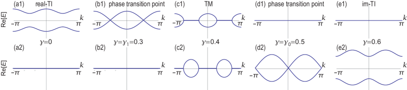
Figure 3: (a1)$\sim$(e1) Real part of the energy and (a2)$\sim$(e2) imaginary part of the energy. (a1) and (a2) for a real-line-gap topological insulator (real-TI) with $\gamma=0$; (b1) and (b2) for a phase transition point with $\gamma=\gamma_{1}=0.3$; (c1) and (c2) for a metal with $\gamma=0.4$; (d1) and (d2) for a phase transition point with $\gamma=\gamma_{0}=0.5$; (e1) and (e2) for an imaginary-line-gap topological insulator (im-TI) with $\gamma=0.6$. We have set $\xi=0.2$ for all figures. See also the caption of Fig.2.

II.2 Non-Hermitian Hamiltonian

We generalize the Hermitian non-Abelian system (2) to a non-Hermitian non-Abelian system, keeping $PT$ symmetry. We consider the Hamiltonian

$$H_{\alpha\beta}^{\prime}\left(k;\gamma,\xi\right)=H_{\alpha\beta}^{\prime}\left(k\right)+i\gamma\sigma_{y}+\xi\sigma_{x}\sin k,$$ (14)

whose eigenenergies are

$$E_{\alpha\beta}^{\prime}\left(k;\gamma,\xi\right)=\frac{\varepsilon_{\alpha}+\varepsilon_{\beta}\pm\sqrt{g(k;\gamma,\xi)}}{2},$$ (15)

with

$$g(k;\gamma,\xi)=\left(\varepsilon_{\alpha}-\varepsilon_{\beta}\right)^{2}-\gamma^{2}+4\xi\left(\varepsilon_{\alpha}-\varepsilon_{\beta}+\xi\right)\sin^{2}k.$$ (16)

We explain the meanings of the $\gamma$ term and the $\xi$ term. The Hamiltonian (14) is Hermitian when $\gamma=0$. When $\xi=0$ in addition, the band structure is highly degenerate as in Fig.2(a1). This degeneracy is resolved by introducing the $\xi$ term as shown in Fig.2(a2). We show the band structure with $\gamma=0$ as a function of $\xi$ in Fig.2(b1). The perfect flat bands at $\varepsilon_{\alpha}$ and $\varepsilon_{\beta}$ become bended and have dispersions. We also show the band structure with $\gamma=0.25$ as a function of $\xi$ in Fig.2(b2).

We show Re[$E_{\alpha\beta}^{\prime}\left(k;\gamma,\xi=0\right)$] in Fig.2(c1) and Im[$E_{\alpha\beta}^{\prime}\left(k;\gamma,\xi=0\right)$] in Fig.2(d1) as a function of $\gamma$. They are real for $|\gamma|\leq\gamma_{0}$ with

$$\gamma_{0}=\frac{\varepsilon_{\alpha}-\varepsilon_{\beta}}{2},$$ (17)

where $PT$ symmetry is preserved. On the other hand, they are complex for $|\gamma|>\gamma_{0}$, and hence $PT$ symmetry is spontaneously broken there. Namely, although the Hamiltonian is $PT$-symmetric, eigenvalues and eigenfunctions are no longer real in the spontaneous symmetry broken phase. We show the real and imaginary parts of the energy as a function of $\gamma$ in Fig.2(c2) and (c2), where the bulk band has a finite width. We also show the real and imaginary parts of the energy as a function of the momentum $k$ in Fig.3, where the bands have dispersions.

Especially, we have

$$E_{\alpha\beta}^{\prime}\left(\frac{\pi}{2};\gamma,\xi\right)=\frac{\varepsilon_{\alpha}+\varepsilon_{\beta}\pm\sqrt{h(\gamma,\xi)}}{2},$$ (18)

with

$$h(\gamma,\xi)=\left(\varepsilon_{\alpha}-\varepsilon_{\beta}+2\xi-2\gamma\right)\left(\varepsilon_{\alpha}-\varepsilon_{\beta}+2\xi+2\gamma\right).$$ (19)

By solving the condition that $E_{\alpha\beta}^{\prime}\left(\frac{\pi}{2};\gamma,\xi\right)$ is complex, or $h(\gamma,\xi)<0$, we find a phase transition point $\gamma_{1}$ in addition to the phase transition point $\gamma_{0}$ as

$$\gamma_{1}=\frac{\varepsilon_{\alpha}-\varepsilon_{\beta}}{2}-\xi=\gamma_{0}-\xi.$$ (20)

When $\xi>0$, the bulk energy is real for $\left|\gamma\right|\leq\gamma_{1}$, complex for $\left|\gamma\right|>\gamma_{1}$. On the other hand, when $\xi<0$, the bulk energy is real for $\left|\gamma\right|\leq\gamma_{0}$, complex for $\left|\gamma\right|>\gamma_{0}$.

II.3 Tight-binding Hamiltonian

The tight-binding Hamiltonian (10) is written in the coordinate space as

$$H_{\alpha\beta}^{\prime}=H_{0}+H_{\gamma}+H_{\xi},$$ (21)

with

$$H_{0} = \frac{\varepsilon_{\alpha}-\varepsilon_{\beta}}{2}\sum_{j=1}^{\ell-1}(\left|\alpha_{j}\right\rangle\left\langle\alpha_{j+1}\right|+\left|\beta_{j}\right\rangle\left\langle\beta_{j+1}\right|,$$ (22)

$$+i\left|\alpha_{j}\right\rangle\left\langle\beta_{j+1}\right|-i\left|\beta_{j}\right\rangle\left\langle\alpha_{j+1}\right|)+\text{h.c.},$$

$$H_{\gamma} = \gamma\sum_{j=1}^{\ell}(\left|\alpha_{j}\right\rangle\left\langle\beta_{j}\right|-\left|\beta_{j}\right\rangle\left\langle\alpha_{j}\right|),$$ (23)

$$H_{\xi} = i\xi\sum_{j=1}^{\ell-1}(\left|\alpha_{j}\right\rangle\left\langle\beta_{j+1}\right|-\left|\beta_{j}\right\rangle\left\langle\alpha_{j+1}\right|)+\text{h.c.},$$ (24)

where the first two terms in $H_{0}$ represent normal hoppings, while the last two terms represent spin-orbit-like imaginary hoppings. The $\xi$ term modifies the spin-orbit-like imaginary hoppings. The $\gamma$ term represents nonreciprocal hoppings, which make the system non-Hermitian.

The tight-binding Hamiltonians for the spectator bands are simply given by

$$H_{j\neq\alpha,\beta}=\sum_{j=1}^{\ell}\varepsilon_{j}\left|j\right\rangle\left\langle j\right|+\sum_{j=1}^{\ell-1}t_{j}\left|j\right\rangle\left\langle j+1\right|+\text{h.c.},$$ (25)

where $\varepsilon_{j}$ is the on-site energy and $t_{j}$ is the hopping parameter.

In this sense, it is enough to consider only the $\alpha$ and $\beta$ bands for an arbitrary $N$ band system. We illustrate the tight-binding model in Fig.1.

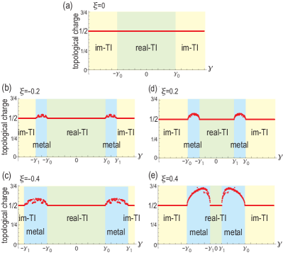
Figure 4: Non-Abelian topological charge marked in red as a function of $\gamma$ for various $\xi$. (a) $\xi=0$, (b) $\xi=-0.2$, (c) $\xi=-0.4$, (d) $\xi=0.2$ and (e) $\xi=0.4$. It is quantized at $1/2$ except for the metallic phase. In the figures, real-TI (im-TI) stands for real(imaginary)-line-gap topological insulator phase.

II.4 Edge states for non-Hermitian model

We illustrate the tight-binding model (21) in Fig.1(b). In a finite chain, two localized states emerge at the edges with the energy

$$E(\xi,\gamma)=\frac{\varepsilon_{\alpha}+\varepsilon_{\beta}}{2}\pm i\gamma$$ (26)

in the presence of the $\gamma$ term and the $\xi$ term. They are degenerate only in the Hermitian limit ($\gamma=0$). In contrasted to the bulk band, the eigenenergy (26) is complex once $\gamma$ is introduced even for the $PT$ symmetric phase. We show Eq.(26) as a function of $\gamma$ in Fig.2. In contrast to the bulk band, the eigenenergy (26) has no $\xi$ dependence: See Figs.2(d1) and (d2).

When $\xi=0$, the eigenfunctions for the edge states $\psi_{\alpha}\left(j\right)$ and $\psi_{\beta}\left(j\right)$ at the $j$ site are perfectly localized at the edges and given by

$$\psi_{\alpha}\left(j\right)=\frac{1}{\sqrt{2}}\delta_{1,j},\qquad\psi_{\beta}\left(j\right)=\frac{-i}{\sqrt{2}}\delta_{1,j}$$ (27)

for the left edge, and

$$\psi_{\alpha}\left(j\right)=\frac{1}{\sqrt{2}}\delta_{\ell,j},\qquad\psi_{\beta}\left(j\right)=\frac{i}{\sqrt{2}}\delta_{\ell,j}$$ (28)

for the right edge. Here, $1$ in $\delta_{1,j}$ represent the left edge, while $\ell$ in $\delta_{\ell,j}$ represents the right edge. The perfectly localized edge states for $\xi=0$ are transformed to edge states with finite penetration depth for $\xi\neq 0$.

II.5 Non-Hermitian Non-Abelian topological charges

We define a non-Hermitian non-Abelian Berry connection or a non-Hermitian Berry-Wilczek-Zee (BWZ) connection byWZ

$$A_{\alpha\beta}^{\text{RL}}\left(\theta\right)=\left\langle\psi_{\alpha}^{\text{R}}\right|\partial_{\theta}\left|\psi_{\beta}^{\text{L}}\right\rangle,$$ (29)

where

$$H\left|\psi_{\alpha}^{\text{L}}\right\rangle=\varepsilon_{\alpha}\left|\psi_{\alpha}^{\text{L}}\right\rangle$$ (30)

is the left eigenfunction, and

$$H^{\dagger}\left|\psi_{\alpha}^{\text{R}}\right\rangle=\varepsilon_{\alpha}\left|\psi_{\alpha}^{\text{R}}\right\rangle$$ (31)

is the right eigenfunction.

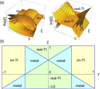
Figure 5: (a) Real and imaginary parts of the bulk-band energy in the $(\gamma,\xi)$ plane. (b) Topological phase diagram in the $(\gamma,\xi)$ plane. Metallic phase appears except for $\xi=0$. In the figure, real-TI (im-TI) stands for real(imaginary)-line-gap topological insulator phase.

We define a non-Hermitian BWZ phase by

$$\Gamma_{\alpha\beta}^{\text{RL}}=\frac{1}{2\pi}\int_{0}^{2\pi}\text{Re}\left[A_{\alpha\beta}^{\text{RL}}\left(\theta\right)\right]d\theta,$$ (32)

which we use as a non-Hermitian non-Abelian topological charge. The eigenfunctions are analytically solved as

$$\left|\psi_{\pm}^{\text{L}}\right\rangle =\frac{1}{\sqrt{\left(\psi_{1}^{\text{L}}\right)^{2}+\left(\psi_{2}^{\text{L}}\right)^{2}}}\left\{\psi_{1}^{\text{L}},\psi_{2}^{\text{L}}\right\},$$ (33)

$$\psi_{1}^{\text{L}} =-\gamma_{0}\cos k\pm\sqrt{\gamma_{0}^{2}-\gamma^{2}+\xi\left(2\gamma+\xi\right)\sin^{2}k},$$ (34)

$$\psi_{2}^{\text{L}} =\gamma-\left(\gamma_{0}+\xi\right)\sin k,$$ (35)

and

$$\left|\psi_{\pm}^{\text{R}}\right\rangle =\frac{1}{\sqrt{\left(\psi_{1}^{\text{R}}\right)^{2}+\left(\psi_{2}^{\text{R}}\right)^{2}}}\left\{\psi_{1}^{\text{R}},\psi_{2}^{\text{R}}\right\},$$ (36)

$$\psi_{1}^{\text{R}} =\gamma_{0}\cos k\pm\sqrt{\gamma_{0}^{2}-\gamma^{2}+\xi\left(2\gamma+\xi\right)\sin^{2}k},$$ (37)

$$\psi_{2}^{\text{R}} =\gamma+\left(\gamma_{0}+\xi\right)\sin k.$$ (38)

When $\gamma=0$ and $\xi=0$, using (33) and (36), we calculate the non-Hermitian BWZ connection (29) numerically and find that

$$A_{\alpha\beta}^{\text{RL}}=\frac{1}{2}\left(\begin{array}[]{cc}0&-1\\ 1&0\end{array}\right),$$ (39)

which leads to the non-Hermitian BWZ phase (32) as

$$\Gamma_{\alpha\beta}^{\text{RL}}=\frac{1}{2}\left(\begin{array}[]{cc}0&-1\\ 1&0\end{array}\right),$$ (40)

where we have explicitly written only the nontrivial $2\times 2$ submatrix within the $N\times N$ matrix. Hence, the topological charges are given by

$$\Gamma_{\alpha\beta}^{\text{RL}}=-\frac{1}{2}L_{\alpha\beta}$$ (41)

with Eq.(1). The topological charges $\Gamma_{\alpha\beta}^{\text{RL}}$ obey essentially the same non-Abelian algebra as $L_{\alpha\beta}$.

When $\gamma\neq 0$ and $\xi=0$, we calculate the non-Hermitian BWZ connection (29) to find that it is no longer a constant. However, the non-Hermitian BWZ phase (32) is calculated as in Eq.(40), and hence the topological charge is quantized as in Eq.(41) for any $\gamma$. Nevertheless, the eigenfunctions as well as the eigenvalues are real (i.e., real-line-gap topological insulator phase) only for $\gamma^{2}\leq\gamma_{0}^{2}$, while the eigenvalues and the eigenfunctions are complex (i.e. imaginary-line-gap topological insulator phase) for $\gamma^{2}>\gamma_{0}^{2}$. Hence, PT symmetry is preserved only for $\gamma^{2}\leq\gamma_{0}^{2}$, and it is spontaneously broken for $\gamma^{2}>\gamma_{0}^{2}$. The system undergoes a phase transition at $\gamma=\pm\gamma_{0}$.

When $\gamma\neq 0$ and $\xi\neq 0$, we have numerically calculated the topological charge (32) with the use of (33) and (36). We have shown the $\left(2,1\right)$ component of the $2\times 2$ matrix $\Gamma_{\alpha\beta}^{\text{RL}}$ for various values of $\xi$ in Fig.4. It is quantized to be 1/2 for $\gamma^{2}\leq\gamma_{1}^{2}$ and $\gamma^{2}>\gamma_{0}^{2}$ when $\xi>0$, while $\gamma^{2}\leq\gamma_{0}^{2}$ and $\gamma^{2}>\gamma_{1}^{2}$ when $\xi<0$, where $\gamma_{1}=\gamma_{0}-\xi$ as in Eq.(20). On the other hand, it is not quantized for the metallic phase that emerges between $\gamma_{0}$ and $\gamma_{1}$, as in Fig.4. It is concluded that the topological charges are quantized and given by Eq.(41) in the insulator phases.

II.6 Topological phase diagram

In non-Hermitian systems, there are line-gap insulators and point-gap insulatorsUedaPRX ; Kawabata in general. In the point-gap insulator, there is a gap in $|E|$. On the other hand, there are two types of line-gap insulators. A real-line gap topological insulator has a gap in Re$\left[E\right]$, while an imaginary-line-gap topological insulator has a gap in Im$\left[E\right]$. We first consider the case $\xi>0$. For $\left|\gamma\right|<\gamma_{1}$, the system is a non-Hermitian line-gap topological insulator along the Re$\left[E\right]$. The systems is metallic for $\gamma_{1}\leq\left|\gamma\right|\leq\gamma_{0}$. For $\left|\gamma\right|>\gamma_{0}$, the system is a non-Hermitian line-gap topological insulator along the Im$\left[E\right]$. If $\xi<0$, the system is a real-line-gap topological insulator for $\left|\gamma\right|<\gamma_{0}$, it is a metal for $\gamma_{0}\leq\left|\gamma\right|\leq\gamma_{1}$ and it is an imaginary-line-gap topological insulator for $\left|\gamma\right|>\gamma_{1}$. We show the topological phase diagram in Fig.5(b). It is consistent with the real and imaginary parts of the energy in the $\gamma$-$\xi$ plane as shown in Fig.5(a).

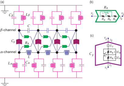
Figure 6: (a) Illustration of the electric circuit corresponding to the lattice in Fig.1(b). The hopping along the $\alpha$-chain ($\beta$-chain) is represented by the inductance $L$ (the capacitance $C$). (b) Negative impedance converter $R_{X}$ represents an imaginary hoppingHofmann . (c) Operational amplifier circuit $C_{\gamma}$ represents a nonreciprocal hoppingNonR .

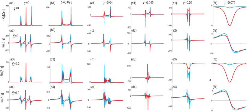
Figure 7: Real and imaginary parts of impedance $Z_{aa}$ at the edge as a function of frequency $\omega$. (a1) $\sim$(a4) Hermitian model with $\gamma=0$. (b1)$\sim$(b4) Non-Hermitian model with $\gamma=0.025$, (c1)$\sim$(c4) with $\gamma=0.04$ (phase transition point $\gamma_{1}$), (d1)$\sim$(d5) with $\gamma=0.045$, (e1)$\sim$(e4) with $\gamma=0.05$ (phase transition point $\gamma_{0}$), and (f1)$\sim$(f4) with $\gamma=0.075$. We have used a finite chain with open boundary condition (red) and periodic boundary condition (cyan). (a1)$\sim$(f2) $\xi=0$. (a3)$\sim$(f4) $\xi=0.2$. We have set $\varepsilon_{\alpha}=1$ and $\varepsilon_{\beta}=1.1$. The length of the chain is 20.

III Electric circuit simulation

An electric circuit is described by the Kirchhoff current law. By making the Fourier transformation with respect to time, the Kirchhoff current law is expressed as

$$I_{a}\left(\omega\right)=\sum_{b}J_{ab}\left(\omega\right)V_{b}\left(\omega\right),$$ (42)

where $I_{a}$ is the current between node $a$ and the ground, while $V_{b}$ is the voltage at node $b$. The matrix $J_{ab}\left(\omega\right)$ is called the circuit Laplacian. Once the circuit Laplacian is given, we can uniquely setup the corresponding electric circuit. By equating it with the Hamiltonian $H$ asTECNature ; ComPhys

$$J_{ab}\left(\omega\right)=i\omega H_{ab}\left(\omega\right),$$ (43)

it is possible to simulate various topological phases of the Hamiltonian by electric circuitsTECNature ; ComPhys ; Hel ; Lu ; EzawaTEC ; EzawaLCR ; Research ; Zhao ; EzawaSkin ; Garcia ; Hofmann ; EzawaMajo ; Tjunc ; NonR . The relations between the parameters in the Hamiltonian and in the electric circuit are determined by this formula.

In the present problem, only the $\alpha$-chain and the $\beta$-chain are active in the tight-binding Hamiltonian as in Fig.1. Thus, we need only a $2\times 2$ matrix. The circuit Laplacian follows from the Hamiltonian (14) as

$$J_{\alpha\beta}^{\prime}\left(k\right)=i\omega\left[\left(\begin{array}[]{cc}-\frac{L}{\omega^{2}}\cos k&f_{+}\\ f_{-}&C\cos k\end{array}\right)+\frac{\varepsilon_{\alpha}+\varepsilon_{\beta}}{2}\mathbb{I}_{2}\right],$$ (44)

with

$$f_{\pm}=\frac{1}{\omega R_{X}}\left(1+\xi\right)\sin k\pm\gamma.$$ (45)

We may design the electric circuit to realize this circuit Laplacian as in Fig.6. The main part consists of the $\alpha$-channel and the $\beta$-channel corresponding to the $\alpha$-chain and the $\beta$-chain in the lattice in Fig.1. Additionally, each node in the $i$-channel is connected to the ground via a set of inductor $L_{i}$ and capacitor $C_{i}$, where $i=\alpha$ or $\beta$, in order to realize the diagonal term $\varpropto(\varepsilon_{\alpha}+\varepsilon_{\beta})$ in Eq.(44).

Hopping terms along the $\alpha$-chain and the $\beta$-chain are described by the diagonal terms in Eq.(44), where $\pm\cos k=\pm(e^{ik}+e^{-ik})/2$ represents the plus (minus) hopping in the tight-bind model. To simulate the positive and negative hoppings in the Hamiltonian, we replace them with the capacitance $i\omega C$ and the inductance $1/i\omega L$, respectively.

Hopping terms across the $\alpha$-chain and the $\beta$-chain are described by the off-diagonal terms $f_{\pm}$ in Eq.(44), which consist of two terms proportional to $\sin k$ and $\gamma$.

(i) The term proportional to $\sin k$ produces the cross hopping, where $\sin k=(e^{ik}-e^{-ik})/2i$ represents an imaginary hopping in the tight-bind model. The imaginary hopping is implemented by a negative impedance converter $R_{X}$ with current inversionHofmann , as is constructed based on an operational amplifier with resistors: See Fig.6(b). The voltage-current relation is given by

$$\left(\begin{array}[]{c}I_{1}\\ I_{2}\end{array}\right)=\frac{1}{R_{X}}\left(\begin{array}[]{cc}-\nu&\nu\\ -1&1\end{array}\right)\left(\begin{array}[]{c}V_{1}\\ V_{2}\end{array}\right),$$ (46)

with $\nu=R_{b}/R_{a}$, where $R_{X}$, $R_{a}$ and $R_{b}$ are the resistances in an operational amplifier. We note that the resistors in the operational amplifier circuit are tuned to be $\nu=1$ in the literatureHofmann so that the system becomes Hermitian, where the corresponding Hamiltonian represents a spin-orbit interaction. It produces the Hamiltonian

$$H=\frac{1}{\omega R_{X}}\left(\begin{array}[]{cc}i&-i\\ i&-i\end{array}\right)$$ (47)

for the Hermitian limit.

(ii) The term $\varpropto\gamma$ produces the nonreciprocal hopping terms, which are vertical hoppings represented by red arrows in Fig.1(b). The nonreciprocal hopping is constructed by a combination of an operational amplifier and capacitorsNonR ,

$$\left(\begin{array}[]{c}I_{ij}\\ I_{ji}\end{array}\right)=i\omega C_{\gamma}\left(\begin{array}[]{cc}-1&1\\ -1&1\end{array}\right)\left(\begin{array}[]{c}V_{i}\\ V_{j}\end{array}\right),$$ (48)

as in Fig.6(c). It corresponds to the Hamiltonian

$$H=C_{\gamma}\left(\begin{array}[]{cc}-1&1\\ -1&1\end{array}\right).$$ (49)

In this way, the tight-binding Hamiltonian for the present non-Hermitian non-Abelian topological system is implemented in the electric circuit given in Fig.6.

III.1 Impedance resonance

The band structure as well as edge states are well observed by impedance resonance, which is definedTECNature ; ComPhys ; Hel by

$$Z_{ab}=V_{a}/I_{b}=G_{ab},$$ (50)

where $G=J^{-1}$ is the Green function. Taking the nodes $a=b$ at an edge, we show the real and imaginary parts of the impedance for a finite chain as a function of $\omega$ in Fig.7, which are marked in red. For comparison, we also show the impedance for a periodic boundary condition in cyan, where the edge states are absent.

We first study the Hermitian case ($\gamma=0$) with $\xi=0$, where the impedance is shown in Fig.7(a1) and (a2). The edge impedance resonance is clear by comparing the periodic boundary condition and the open boundary condition. There are only two bulk peaks in cyan at Re[$E_{\alpha\beta}^{\prime}\left(k;\gamma,\xi\right)$]. On the other hand, there is an additional peak in red due to the edge states between two bulk peaks, as corresponds to Fig.2(a1).

Next, we show the impedance for various nonreciprocity $\gamma$ with $\xi=0$ in Fig.7(a1)$\sim$(f1) and (a2)$\sim$(f2). The edge impedance resonance rapidly decreases as the increase of $\gamma$, as shown in Fig.7(b1). This is due to the imaginary contribution in Eq.(26). Then, the distance between two bulk peaks becomes narrower, which is consistent with Re[$E_{\alpha\beta}^{\prime}\left(k;\gamma,\xi=0\right)$] as shown in Fig.2(c1). The two bulk peaks merge into one peak at the spontaneous $PT$ symmetry breaking point $\gamma_{0}$, as shown in Fig.7(e1). The bulk impedance resonance is very strong due to the gap closing of the bulk band. We also observe the edge impedance resonance in the imaginary-line gap topological insulating phase, where the impedance resonance is weak comparing to Fig.7(a1) as shown in Fig.7(f1). This is also the imaginary contribution in Eq.(26).

We also show the impedance for finite $\xi$ in Fig.7(a3)$\sim$(f3) and (a4)$\sim$(f4), as corresponds to Fig.2(c2). The bulk impedance peaks become broad, which reflects the broadening of the bulk bands. As a result, the edge impedance peak becomes clearer as in Fig.7(a3) in comparison to Fig.7(a1). There are strong cyan resonances at the phase transition point $\gamma_{1}$ point as shown in Fig.7(c3) and (c4). It is due to the gap closing of the bulk band. In Fig.7(d3) and (d4), the impedance structure is complicated, which reflects the metallic band structure. The effect of the $\xi$ term is negligible for the imaginary-line-gap topological phase as shown in Fig.7(f3) and (f4) since the peak of the impedance is broad even for $\xi=0$ in Fig.7(f1) and (f2). Here, note that $\xi$ appears only in the form of $(1+\xi)$ in Eq.(45).

IV Conclusion

We have proposed a non-Hermitian non-Abelian topological insulator model by imposing $PT$ symmetry in one dimension. It describes a real-line-gap topological insulator with real eigenvalues in the Hermitian limit. The system undergoes a spontaneous breakdown of $PT$ symmetry as the non-Hermitian term increases, and turns out to describe an imaginary-line-gap topological insulator, when the bulk bands are perfectly flat. When we introduce a bulk bending term, there are two phase transitions with the emergence of a metal with complex eigenvalues between the above two topological insulators. Finally, we have presented how to construct these models in electric circuits. We have shown that the spontaneous $PT$ symmetry breaking as well as topological edge states are well signaled by measuring the frequency dependence of the impedance.

References

- (1) M. Z. Hasan and C. L. Kane, Rev. Mod. Phys. 82, 3045 (2010).
- (2) X.-L. Qi and S.-C. Zhang, Rev. Mod. Phys. 83, 1057 (2011).
- (3) Q. Wu, A. A. Soluyanov, T. Bzdusek, Science 365, 1273 (2019)
- (4) A. Tiwari and T. Bzdušek, Phys. Rev. B 101, 195130 (2020)
- (5) E. Yang, B. Yang, O. You, H.-c. Chan, P. Mao, Q. Guo, S. Ma, L. Xia, D. Fan, Y. Xiang, S. Zhang, Phys. Rev. Lett. 125, 033901 (2020)
- (6) P. M. Lenggenhager, X. Liu, S. S. Tsirkin, T. Neupert and T. Bzdusek, arXiv:2008.02807
- (7) Q. Guo, T. Jiang, R.-Y. Zhang, L. Zhang, Z.-Q. Zhang, B. Yang, S. Zhang, C. T. Chan, Nature 594, 195 (2021)
- (8) A. Bouhon, Q. Wu, R.-J. Slager, H. Weng, O. V. Yazyev and T. Bzdusek, Nature Physics 16, 1137 (2020)
- (9) D. Wang, B. Yang, Q. Guo, R.-Y. Zhang, L. Xia, X. Su, W.-J. Chen, J. Han, S. Zhang, C. T. Chan, Light: Science & Applications 10, 83 (2021)
- (10) H. Park, S. Wong, X. Zhang, S. S. Oh, arXiv:2102.12546
- (11) Bin Jiang, Adrien Bouhon, Zhi-Kang Lin, Xiaoxi Zhou, Bo Hou, Feng Li, Robert-Jan Slager, Jian-Hua Jiang, arXiv:2104.13397
- (12) M. Wang, S. Liu, Q. Ma, R.-Y. Zhang, D. Wang, Q. Guo, B. Yang, M. Ke, Z. Liu, and C. T. Chan, arXiv:2106.06711
- (13) T. Jiang, Q. Guo, R.-Y. Zhang, Z.-Q. Zhang, B. Yang, C. T. Chan, arXiv:2106.16080
- (14) B. Peng, A. Bouhon, B. Monserrat, R.-J. Slager, arXiv:2105.08733
- (15) C. M. Bender and S. Boettcher, Phys. Rev. Lett. 80, 5243 (1998).
- (16) R. El-Ganainy, K. G. Makris, M. Khajavikhan, Z. H. Musslimani, S. Rotter and D. N. Christodoulides, Nat. Physics 14, 11 (2018).
- (17) C. M. Bender, D. C. Brody, and H. F. Jones, Phys. Rev. Lett. 89, 270401 (2002).
- (18) S. Malzard, C. Poli, H. Schomerus, Phys. Rev. Lett. 115, 200402 (2015).
- (19) V. V. Konotop, J. Yang, and D. A. Zezyulin, Rev. Mod. Phys. 88, 035002 (2016).
- (20) T. Rakovszky, J. K. Asboth, and A. Alberti, Phys. Rev. B 95, 201407(R) (2017).
- (21) B. Zhu, R. Lu and S. Chen, Phys. Rev. A 89, 062102 (2014).
- (22) S. Yao and Z. Wang, Phys. Rev. Lett. 121, 086803 (2018).
- (23) L. Jin and Z. Song, Phys. Rev. B 99, 081103 (2019).
- (24) S.-D. Liang and G.-Y. Huang, Phys. Rev. A 87, 012118 (2013).
- (25) D. Leykam, K. Y. Bliokh, Chunli Huang, Y. D. Chong, and Franco Nori, Phys. Rev. Lett. 118, 040401 (2017).
- (26) S. Lieu, Phys. Rev. B 97, 045106 (2018).
- (27) Z. Gong, Y. Ashida, K. Kawabata, K. Takasan, S. Higashikawa and M. Ueda, Phys. Rev. X 8, 031079 (2018).
- (28) E. Cobanera, A. Alase, G. Ortiz, L. Viola, Phys. Rev. B 98, 245423 (2018).
- (29) H. Jiang, C. Yang and S. Chen, Phys. Rev. A 98, 052116 (2018)
- (30) A. Ghatak, T. Das, J. Phys.: Condens. Matter 31, 263001 (2019).
- (31) Y. Ashida, Z. Gong, M. Ueda, Advances in Physics 69, 3 (2020)
- (32) A. Mostafazadeh, J. Math. Phys 43, 205 (2002).
- (33) C. E. Ruter, K. G. Makris, R. El-Ganainy, D. N. Christodoulides, M. Segev and D.Kip, Nat. Phys. 6, 192 (2010)
- (34) C. Yuce, Physics Letters A 379, 12213 (2015).
- (35) L. Feng, R. El-Ganainy and L. Ge, Nature Photonics 11, 752 (2017).
- (36) S. Weimann, M. Kremer, Y. Plotnik, Y. Lumer, S. Nolte, K. G. Makris, M. Segev, M. C. Rechtsman and A. Szameit, Nature Materials 16, 433 (2017)
- (37) N. Hatano and D. R. Nelson, Phys. Rev. Lett. 77, 570 (1996): Phys. Rev. B 56, 8651 (1997): Phys. Rev. B 58, 8384 (1998).
- (38) F. Wilczek and A. Zee Phys. Rev. Lett. 52, 2111 (1984)
- (39) K. Kawabata, K. Shiozaki, M. Ueda, and M. Sato, Phys. Rev. X 9, 041015 (2019).
- (40) S. Imhof, C. Berger, F. Bayer, J. Brehm, L. Molenkamp, T. Kiessling, F. Schindler, C. H. Lee, M. Greiter, T. Neupert, R. Thomale, Nat. Phys. 14, 925 (2018).
- (41) C. H. Lee , S. Imhof, C. Berger, F. Bayer, J. Brehm, L. W. Molenkamp, T. Kiessling and R. Thomale, Communications Physics, 1, 39 (2018).
- (42) T. Helbig, T. Hofmann, C. H. Lee, R. Thomale, S. Imhof, L. W. Molenkamp and T. Kiessling, Phys. Rev. B 99, 161114 (2019).
- (43) Y. Lu, N. Jia, L. Su, C. Owens, G. Juzeliunas, D. I. Schuster and J. Simon, Phys. Rev. B 99, 020302 (2019).
- (44) K. Luo, R. Yu and H. Weng, Research (2018), ID 6793752.
- (45) E. Zhao, Ann. Phys. 399, 289 (2018).
- (46) M. Ezawa, Phys. Rev. B 98, 201402(R) (2018).
- (47) M. Serra-Garcia, R. Susstrunk and S. D. Huber, Phys. Rev. B 99, 020304 (2019).
- (48) T. Hofmann, T. Helbig, C. H. Lee, M. Greiter, R. Thomale, Phys. Rev. Lett. 122, 247702 (2019).
- (49) M. Ezawa, Phys. Rev. B 100, 045407 (2019)
- (50) M. Ezawa, Phys. Rev. B 102, 075424 (2020)
- (51) M. Ezawa, Phys. Rev. B 99, 201411(R) (2019).
- (52) M. Ezawa, Phys. Rev. B 99, 121411(R) (2019).
- (53) T. Helbig, T. Hofmann, S. Imhof, M. Abdelghany, T. Kiessling, L. W. Molenkamp, C. H. Lee, A. Szameit, M. Greiter, R. Thomale, Nature Physics 16, 747 (2020)