Fitting infrared ice spectra with genetic modelling algorithms

Abstract

Context. A variety of laboratory ice spectra simulating different chemical environments, ice morphology as well as thermal and energetic processing are demanded to provide an accurate interpretation of the infrared spectra of protostars. To answer which combination of laboratory data best fit the observations, an automated statistically-based computational approach becomes necessary.

Aims. To introduce a new approach, based on evolutionary algorithms, to search for molecules in ice mantles via spectral decomposition of infrared observational data with laboratory ice spectra.

Methods. A publicly available and open-source fitting tool, called ENIIGMA (dEcompositioN of Infrared Ice features using Genetic Modelling Algorithms), is introduced. The tool has dedicated Python functions to carry out continuum determination of the protostellar spectra, silicate extraction, spectral decomposition and statistical analysis to calculate confidence intervals and quantify degeneracy. As assessment of the code, fully blind and fully sighted tests were conducted with known ice samples and constructed mixtures. Additionally, a complete analysis of the Elias 29 spectrum was performed and compared with previous results in the literature.

Results. The ENIIGMA fitting tool can identify the correct ice samples and their fractions in all checks with known samples tested in this paper. In the cases where Gaussian noise was added to the experimental data, more robust genetic operators and more iterations became necessary. Concerning the Elias 29 spectrum, the broad spectral range between 2.5$-$20 $\mu$m was successfully decomposed after continuum determination and silicate extraction. This analysis allowed the identification of different molecules in the ice mantle, including a tentative detection of CH₃CH₂OH.

Conclusions. The ENIIGMA is a toolbox for spectroscopy analysis of infrared spectra that is well-timed with the launch of the James Webb Space Telescope. Additionally, it allows for exploring different chemical environment and irradiation field in order to correctly interpret the astronomical observations.

1 Introduction

Characterizing the composition of astrophysical ice mantles in the interstellar medium (ISM) is crucial for understanding the chemical evolution of Young Stellar Objects (YSOs). With this goal, systematic studies in the infrared (IR) with ground- and space-based telescopes (e.g., Chiar et al., 1995; Schutte et al., 1996; Gibb et al., 2000; Pontoppidan et al., 2003a; Boogert et al., 2008; Zasowski et al., 2009; Thi et al., 2011; Öberg et al., 2011) aided by laboratory experiments simulating diverse chemical environments and irradiation fields (e.g., Gerakines et al., 1995; Schutte et al., 1993; Palumbo et al., 1998; Watanabe & Kouchi, 2002; Fuchs et al., 2009; Pilling et al., 2010; Linnartz et al., 2015; Terwisscha van Scheltinga et al., 2018; Rachid et al., 2020; Ioppolo et al., 2021) have pushed forward the frontiers of knowledge about the composition of interstellar ices.

The Infrared Space Observatory (ISO) allowed for the first systematic studies of ices in star-forming regions (e.g. Schutte et al., 1996; van Dishoeck et al., 1998). These observations revealed the presence of H₂O, NH₃, and CH₄, as well as allowed to infer the synthesis of new chemical species such as CH₃OH and NH${}_{4}^{+}$, both byproducts of heating and energetic processing by photons and cosmic rays (Gibb et al., 2000, 2004). Tentative assignments of CH₃CHO (acetaldehyde) and HCOOH (formic acid) relying on the absorption features at 7.24 $\mu$m and 7.41 $\mu$m were made by Schutte et al. (1999). However, the strong bands at 5.80 $\mu$m associated with these two molecules have not been unequivocally detected yet, and, therefore the presence of these molecules is still under debate.

The Spitzer Space Telescope improved in sensitivity compared to ISO allowed ice surveys toward low-mass star-forming regions, background stars and high-UV environments (e.g., Bergin et al., 2005; Whittet et al., 2009; Reach et al., 2009; Boogert et al., 2013). Systematic analysis of the 5$-$8 $\mu$m absorption complex, CH₄ band at 7.7 $\mu$m, CO₂ bending mode at 15.2 $\mu$m, as well as NH₃ and CH₃OH absorption features at 9.01 $\mu$m and 9.74 $\mu$m, were performed in Boogert et al. (2008); Öberg et al. (2008); Pontoppidan et al. (2008) and Bottinelli et al. (2010), respectively. All used a phenomenological approach and/or analytical function decomposition to estimate environment-dependent variations, in order to avoid degenerated solutions in characterizing the ice morphology. A statistical analysis of the ice column density and abundance with respect to H₂O in these four studies was done by Öberg et al. (2011), who concluded that except in the case of CO, CO₂ and CH₄ (the most volatile species), there is no significant statistical abundance variation between low- and high-mass YSOs in the case of OCN^-, CH₃OH, and the broad residual component, C5, described in Boogert et al. (2008). In the case of background sources, however, the abundances of CO and CO₂ are similar to the low-mass YSOs and higher than the high-mass YSOs by a factor of around 3.4 (Boogert et al., 2013, 2015).

Considering pathways and morphology, the analysis of Spitzer observations demonstrated that CO₂, NH₃, and CH₄ ice abundances do not vary significantly with respect to H₂O ice, which indicates co-formation (Öberg et al., 2011). On the contrary, the same work shows that CH₃OH and CO ices vary by order-of-magnitude relative to water ice, thus indicating different formation pathways. NH${}_{4}^{+}$ is anti-correlated with H₂O, likely due to the high desorption temperature compared to other volatiles (Greenberg & D’Hendecourt, 1985). In the case of CO and CO₂, there is evidence in support of cosmic-ray processing, given the abundance ratio CO:CO₂, as well as thermal evolution, that is mainly seen by the CO₂ bending mode splitting at 15.2 $\mu$m (Pontoppidan et al., 2008). Attempts at assigning more complex molecules such as HCOOH, CH₃CHO and CH₃CH₂OH were also made by Öberg et al. (2011), although they are still relying on the absorption features between 7$-$8 $\mu$m.

The main disadvantage of the phenomenological approach is the limited information about ice morphology and the a priori assumption of carriers associated with the absorption bands. In addition, these methods are usually limited to a short wavelength range to address a small set of spectral components (e.g. 3-5; Pontoppidan et al., 2003b; Thi et al., 2006; Boogert et al., 2008). Other approaches combining laboratory ice spectra to fit the observed spectra have been adopted in previous works (Merrill et al., 1976; Gibb et al., 2004; Thi et al., 2006; Zasowski et al., 2009; Suutarinen, 2015). Although the degeneracies are high in these methods, some issues in the direct comparison of the observations with the experimental data were revealed, as is the case of the absorption peak at 6 $\mu$m attributed to H₂O ice, found to be deeper than the features at 3 $\mu$m and 13 $\mu$m (Schutte et al., 1996; Keane et al., 2001), as well as the nature of the peaks at 3.55 $\mu$m and 6.85 $\mu$m, that cannot be only attributed to CH₃OH ice (Dartois & d’Hendecourt, 2001; Schutte & Khanna, 2003; Bottinelli et al., 2010).

In order to allow exploitation of large data-sets of laboratory ice spectra to identify and quantify molecules in ice mantles observed toward YSOs, a new computational code for spectral analysis is presented in this paper. The code uses genetic modelling algorithm (Holland, 1975) to decompose IR spectra of protostars using a linear combination of laboratory data themselves. The use of evolutionary algorithms have successfully been used in the literature to derive the dust composition in asymptotic giant branch (AGB) stars (Baier et al., 2010), as well as to derive physical properties of protostars (Woitke et al., 2016). This paper is laid out as follows: Section 2 list the public databases containing ice spectra used in this work and Section 3 details the code methodology. The accuracy and performance tests of this tool are discussed in Section 4, and an application to a real source, the Class I protostar Elias 29 is shown in Section 5. A summary of the capabilities of the ENIIGMA fitting tool and the results of the Elias 29 spectral analysis are given in Section 6.

2 The ENIIGMA fitting tool

The ENIIGMA (“dEcompositioN of Infrared Ice features using Genetic Modelling Algorithm”) fitting tool aims for the analysis of observational spectra containing ice absorption features. As a general overview, the structure of this tool is split into three major modules; the first provides Python functions to calculate the continuum spectral energy distribution (SED) of YSOs spectra and silicate feature removal. The second focuses on the unbiased spectral decomposition using a linear combination of laboratory ice spectrum. The third offers a statistical analysis of the fits such as confidence intervals and degeneracy quantification. The ENIIGMA fitting tool documentation and download instructions are publicly available at https://eniigma-fitting-tool.readthedocs.io.

In the first module, the ENIIGMA makes use of previous techniques available in the literature for the continuum determination (e.g. Boogert et al., 2000) and silicate removal from a template (e.g., Bottinelli et al., 2010). The second and third module stand the novelty of the code that uses genetic modelling algorithms to search for the optimal solution in a large problem space followed by a robust statistical analysis of the results. Global optimization is a mathematical method that aims to search for the best overall solution providing the maximum likelihood among the parameters. This method is unbiased in the sense that a large sample of ice spectra is tested without targeting any particular species, and the final statistically-based decision of the best fit is made. In the context of ice observations in space, it allows us to explore a significant amount of IR laboratory data and decide for the best ice components. A flowchart of the entire procedure is shown in Figure 1, and the different step are detailed in the next sections.

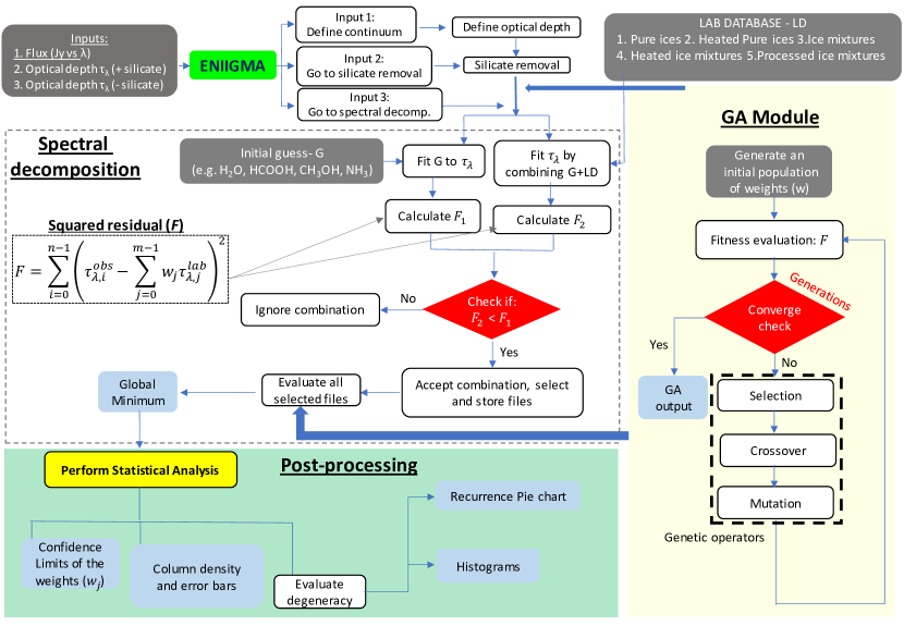
Figure 1: Flowchart of the ENIIGMA fitting tool. The light grey dashed box highlights the steps during the spectral decomposition. The light yellow region highlights the Genetic Algorithm (GA) module, whereas the light green region shows the steps performed during the post-processing statistical analysis. The small grey boxes indicate the input data requested by the tool. Small blue boxes are the output data. White boxes indicate the processes performed in each step.

2.1 Input data, continuum determination and optical depth

The ENIIGMA fitting tool works with three types of input data. The first possibility is to work with observed spectra representing the flux in units of Jy. The second possibility is to use spectra in an optical depth scale – including the silicate features at 9.8 $\mu$m and 18 $\mu$m. Finally, it is possible to provide the tool with spectra where the silicate features have been removed. The file format and structure must be ASCII (American Standard Code for Information Interchange), with three columns, containing the wavelength in micrometres, flux or optical depth and the errors, respectively.

The accurate analysis of the chemical composition and column densities of ices in star-forming regions depends on the subtraction of continuum SED. However, determining an accurate continuum SED of YSOs is challenging because of the large width of the ice and silicate features. Wavelengths shortwards of 5 $\mu$m are better constrained because of the lack of ice bands at the K-band and the narrow features of CO₂ and CO ices at 4.27 and 4.67 $\mu$m, respectively. Some methods for the continuum determination shortwards of 4 $\mu$m have been adopted in the literature such as the near-IR excess removal by using the Kurucz stellar atmosphere models (e.g. Pontoppidan et al., 2004) and a linear combination of black-bodies to fit near- and mid-IR photometric data (e.g. Ishii et al., 2002; Moultaka et al., 2004; Perotti et al., 2020, 2021). Both methods not only provide the flux continuum, but also physical properties such as near-IR extinction or effective temperature.

The continuum above 5 $\mu$m, on the other hand, is much less constrained even though short-wavelength data is available. The entire range between 5$-$30 $\mu$m is dominated by multiple broad and narrow absorption and emission features associated to ices and polycyclic aromatic hydrocarbons (PAHs), respectively (see reviews by Tielens, 2008; Boogert et al., 2015). Hydrogenated amorphous carbon (HAC), or more generally a-C(:H), is another class of material observed toward Galactic Center sources with multiple features in this spectral range (Chiar et al., 2000; Jones, 2012). Toward YSOs, a-C(:H) has been attributed to the absorption bands at 3.47 $\mu$m, 6.85 $\mu$m and 7.25 $\mu$m (e.g., Gibb et al., 2004; Alata et al., 2014). Nevertheless, the profile at 3.47 $\mu$m shows a good correlation with the water ice band at 3 $\mu$m, thus suggesting this band is associated with volatile chemical species, instead (e.g., Brooke et al., 1999; Dartois et al., 2002; Boogert et al., 2015). The strong feature at 6.85 $\mu$m observed toward YSOs, has also been excluded as a potential carrier of a-C(:H) - as it is observed in a similar wavelength in the diffuse ISM - due to the absence of the strong feature at 3.40 $\mu$m (Boogert et al., 2015). The 6.85 $\mu$m band has also been attributed to the CO${}_{3}^{-}$ ion in minerals, but the lack of absorption bands at short or long wavelengths discard this possibility (e.g. Tielens & Allamandola, 1987; Schutte et al., 1996; Boogert et al., 2008, 2015). Finally, the feature at 7.25 $\mu$m can be associated with HCOOH (Schutte et al., 1999), ethanol (CH₃CH₂OH; Öberg et al., 2011; Terwisscha van Scheltinga et al., 2018) and aminomethanol (NH₂CH₂OH; Bossa et al., 2009). However, Jones (2016) discuss that the other compounds containing C$=$O bonds (e.g., ketone, organic carbonate), could be present in the grains before or at the onset of ice mantle formation, and therefore, the bands at 3.47 $\mu$m, 6.85 $\mu$m and 7.25 $\mu$m, could be consistent with carbonyl functional groups. Because of all of these uncertainties, a low-order polynomial fit has usually been used to trace the continuum between the 5 and 32 $\mu$m spectral range (e.g. Gibb et al., 2000, 2004; Pontoppidan et al., 2005; Boogert et al., 2008; Zasowski et al., 2009; Boogert et al., 2011; Öberg et al., 2011; Noble et al., 2013, 2017).

Given that context, the low-order polynomial and blackbody combination methods are incorporated in the ENIIGMA tool for the continuum determination of the observational flux. In the polynomial approach, the function below is used:

$$F_{\mathrm{poly}}(\lambda)=\sum_{k=0}^{n}a_{k}\lambda^{k},$$ (1)

where $a_{k}$ are the constants, $\lambda^{k}$ the wavelength and $k$ the polynomial order. The second method adopts a sum of blackbodies, given by:

$$F_{\mathrm{BB}}(\lambda,T)=\sum_{i=1}^{m}f_{i}\frac{2hc^{2}}{\lambda^{5}}\left(\mathrm{exp}\left[\frac{hc}{\lambda k_{\mathrm{B}}T_{i}}\right]-1\right)^{-1}$$ (2)

where $f_{i}$ is a scale factor, $h$ the Planck’s constant, $c$ the light velocity, $k_{B}$ the Boltzmann’s constant, $\lambda$ the wavelength and $T_{i}$ the temperature of each blackbody.

Once the continuum SED is determined from Equations 1 or 2, the observed spectrum ($F_{\lambda}^{obs}$) is converted to an optical depth scale using the following equation:

$$\tau_{\lambda}^{obs}=-\mathrm{ln}\left(\frac{F_{\lambda}^{obs}}{F_{\lambda}^{cont}}\right)$$ (3)

2.2 Silicate removal

The spectral range between 8$-$25 $\mu$m is dominated by strong and weaker silicate absorption features at 9.7 $\mu$m and 18 $\mu$m, respectively. However, other functional groups associated with simple or complex molecules are also blended in the silicate band at 9.7 $\mu$m. Some examples are ammonia (9.01 $\mu$m; $\nu_{2}$ umbrella vibrational mode) and methanol (9.74 $\mu$m; $\nu_{4}$ stretching vibrational mode of C$-$O bond) as discussed in Boogert et al. (2008) and Bottinelli et al. (2010). Additionally, ethanol (CH₃CH₂OH) also shares the C$-$O stretching mode at 9.51 $\mu$m with the silicate broad profile.

A proper removal of the silicate feature is therefore critical, although not straightforward. Different methodologies have been used in the literature, such as the local continuum and silicate spectrum template of sources toward the Galactic Center (e.g., the GCS 3 silicate absorption profile, taken from Kemper et al., 2004). In Boogert et al. (2008), this absorption feature is narrower compared to the observed silicate band of HH 46 IRS. As a consequence, when the GCS 3 absorption band is used for the silicate removal, a significant residual is left between 8$-$10 $\mu$m. A systematic study by van Breemen et al. (2011) shows that such an IR excess is absent in the sightline of the diffuse interstellar medium, while it is present toward molecular clouds. Although this difference can be associated with ice growth in some cases (e.g., H₂O, NH₃ and CH₃OH; Ossenkopf & Henning, 1994; Boogert & Ehrenfreund, 2004; Boogert et al., 2008; McClure, 2009; Bottinelli et al., 2010), it is also observed toward sources with weak or absent absorption of these molecules at other wavelengths (e.g., SSTc2d_J182835.8+002616; van Breemen et al., 2011). In this regard, such an IR excess is likely due to the chemical composition of the dust, most specifically, the combination of magnesium-rich pyroxene-type (MgSiO₃) and amorphous olivine-type (Mg₂SiO₄) silicates. Further evidence that the silicate band is not associated with only one composition has been found by Poteet et al. (2015), that fitted the silicate profile with a linear combination of amorphous silicates, in particular Mg₂SiO₄, MgFeSiO₄, and MgSiO₃. This study indicates that although small, variations in the silicate band shape cannot be ruled out. In the same framework, the THEMIS (The Heterogeneous dust Evolution Model for Interstellar Solids) code also uses amorphous olivine-type and pyroxene-type silicates with inclusions of iron compounds and a-C(:H) to interpret the observed absorption bands in the diffuse ISM (Jones et al., 2013). Additionally, the effects of dust evolution from the diffuse ISM to denser regions can be addressed with the THEMIS code (e.g., Köhler et al., 2015; Jones et al., 2017).

The debate about the nature (geometry, size and composition) of the silicate feature toward galactic center sources and protostars is still to be clarified by high-quality data that will be provided by the upcoming James Webb Space Telescope observations. To avoid the uncertainties underlying the silicate feature, the ENIIGMA fitting tool assumes a synthetic silicate profile. This method is similar to the silicate template scaling approach used by Bottinelli et al. (2010). The steps adopted here are the following: (I) the observational GCS 3 silicate profile is scaled to match the bands at 9.7 $\mu$m and 18 $\mu$m (same as Bottinelli et al., 2010); (II) these two silicate bands are decomposed into six Gaussian components (three for each band); (III) a small variation of the width and height of the six Gaussian components are performed to match the YSO silicate profile. The synthetic silicate is therefore given by the following the set of equations:

$$G(\lambda;A,\lambda_{0},\sigma) = \frac{A}{\sigma\sqrt{2\pi}}\mathrm{exp}\left[-\frac{(\lambda-\lambda_{0})^{2}}{2\sigma^{2}}\right]$$ (4a)

$$\tau_{\lambda}^{ss} = \sum_{\begin{subarray}{c}i=0\\ j=0\end{subarray}}^{\begin{subarray}{c}m-1\\ n-1\end{subarray}}G(\lambda^{i},\lambda_{0}^{j})$$ (4b)

$$\lambda_{0}(\mu m) = 8.3,9.7,11.2,16.2,18.0,20.8$$ (4c)

where $G(\lambda;A,\lambda_{0},\sigma)$ is the Gaussian function, $\tau_{\lambda}^{ss}$ is the synthetic silicate (ss) optical depth, $\lambda_{0}$ are the fixed peak positions of each component, $A$ is the amplitude and $\sigma$ is the width of the components. Note that in this approach only $A$ and $\sigma$ are allowed to vary. This method assumes that the silicate width of protostars is substantially caused by the dust chemical composition as shown by van Breemen et al. (2011) and the ice features are not affected.

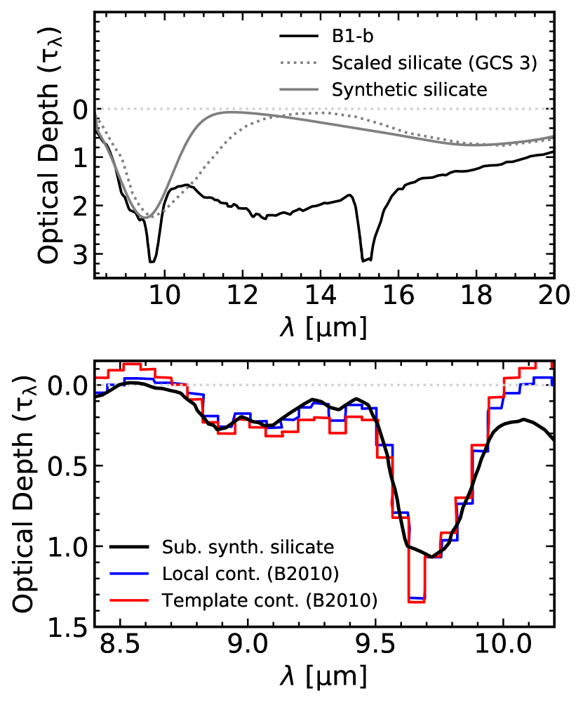
Figure 2: Illustration of the silicate removal with the synthetic silicate method. Top: The B1-b optical depth is shown by the black solid line, whereas the dashed and solid lines are the scaled GCS 3 silicate profile and the synthetic silicate feature, respectively. Bottom: Residual optical depth after synthetic silicate removal (black line). The blue and red colours show the residual optical depth after local and template continuum methods, respectively (See text for details; Bottinelli et al., 2010).

Figure 2 shows an example of how the synthetic silicate method is applied to an observational spectrum. As shown in the top panel, the GCS 3 silicate profile is scaled to the peak at 9.7 $\mu$m of the B1-b spectrum taken from Boogert et al. (2008) (Step I). After steps (II) and (III), the synthetic silicate feature is calculated to match the observational spectrum. The band at 18 $\mu$m, however, is less deep than the observed profile. In the bottom panel, the residual spectrum of B1-b after the silicate removal is shown and compared with the residual spectra taken from Bottinelli et al. (2010). To extract the 9.7 $\mu$m silicate feature, the authors used the local and template continuum methods. Briefly, the local continuum mimics the silicate feature by a short-range polynomial fit, in particular, the intervals between 8.25$-$8.75, 9.23$-$9.37 and 9.98$-$10.4 $\mu$m. Conversely, the template continuum uses empirical profiles separated into three general categories, namely, (1) sources with a straight 8 $\mu$m wing, (2) sources with a curved 8 $\mu$m wing, and (3) sources with a rising 8 $\mu$m wing (“emission” sources). In the case of B1-b source, the curved 8 $\mu$m wing has been used. As mentioned by Bottinelli et al. (2010), the template method is not suitable to fit the 9.7 $\mu$m silicate feature toward all YSOs in their sample, and the local continuum approach was adopted instead. However, this method provides narrow bands for the feature at 9 $\mu$m, often associated with NH₃ ice, then in the template method (Öberg et al., 2011). From an eyeball comparison, one can note that the synthetic silicate method introduced in this paper agrees very well with the methods adopted by Bottinelli et al. (2010). In this way, it can be an alternative to the local continuum method when the template profile is not available. It is worth noting than an advantage of the synthetic silicate method is that it provides the silicate extraction of both 9.7 $\mu$m and 18 $\mu$m bands simultaneously, which allows a better analysis of the H₂O libration band at around 13 $\mu$m. Despite the challenges, new laboratory data combining ice and dust could provide a better understanding of the link between ice and dust in star-forming regions. With this goal, Potapov et al. (2018, 2021) have measured spectrum and optical constants of silicate (MgSiO₃) and H₂O ice, and showed that this experimental data can partially fit the 3 $\mu$m of some astronomical objects.

2.3 Laboratory ice spectra and databases

In order to build an internal database of experimental data for the ENIIGMA to decompose the spectra of YSOs, a data-set of around 100 laboratory ice spectra were compiled from publicly online databases which are listed below:

• NASA Ames: The Astrophysics & Astrochemistry Lab at NASA Ames Research Center

• Leiden DB: Leiden Ice Database

• UNIVAP: Laboratorio de Astroquimica & Astrobiologia da UNIVAP

The ice samples compiled in this paper were recorded in transmittance ($T$) or absorbance ($A$) mode using Fourier Transform Infrared Spectrometer (FTIR). All spectra in transmittance scale were converted to absorbance using the equation $A=-\mathrm{log_{10}}(T)$. In the absorbance scale, the ice spectra can be converted to optical depth using following the equation (D’Hendecourt & Allamandola, 1986):

$$\tau_{\lambda}^{lab}=2.3\cdot A_{\lambda}.$$ (5)

In addition to the compiled data, two IR spectra containing organic residue material (henceforth: residue) at high temperature (¿ 100 K) were taken from the literature. Residue is produced with or without UV irradiation of the ice mixture samples and subsequent warm-up until room temperature (300 K). In particular, the spectra taken from Schutte & Khanna (2003) are HNCO:NH₃ heated until 120 K without energetic processing and H₂O:CO₂:NH₃:O₂ irradiated with UV and heated until 200 K. In common, these experiments identified the ammonium ion (NH${}_{4}^{+}$) formation, a likely carrier of the absorption band at 6.85 $\mu$m in YSOs spectra (Schutte et al., 1996).

Accurate baseline correction of the laboratory data is required to avoid misinterpretations of the carriers. As an example, the band at 5.85 $\mu$m that has been attributed to HCOOH by Schutte et al. (1996, 1999), was put into question by Boogert et al. (2008) and Öberg et al. (2011) because of unreliable laboratory baselines. Instead, ethanol (CH₃CH₂OH) was proposed as the carrier by those authors. To avoid this issue, the baselines of the data compiled in this paper were checked and corrected when necessary. Appendix A lists the data-sets used in this paper and the reference from where the data were taken. In brief, these ice data are grouped by common characteristics, such as (i) pure, (ii) pure and heated, (iii) heated mixtures, (iv) irradiated mixtures and (v) residue.

2.4 Genetic Algorithm Module

Inspired by the theory of natural selection and biological evolution, the genetic algorithms (GA) aim to provide a global optimization process for a proposed problem. For clarification purposes, the GA nomenclature is briefly explained: (i) gene corresponds to the value of a parameter (e.g., scaling factor of the ice spectrum to match the observation), (ii) chromosome is a set of values proposed as a solution of the parameters, (iii) fitness function is the criteria to evaluate the fit (e.g., squared residual, reduced $\chi^{2}$), selection is the election of the best parameters out of the entire set of potential solutions (chromosome) used to generate improved values, (iv) crossover is the mixing of values from two distinct solutions in order to create a new solution, (v) mutation is a small variation of one or more parameters (gene), (vi) global minimum is the optimal solution of the parameters and (vii) generation corresponds to an interaction where potential solutions are tested.

The GA module implemented in the ENIIGMA fitting tool is build on Pyevolve (Perone, 2009), an open-source and extensible library dedicated to perform evolutionary computation in Python programming language. The GA computation is composed of three main characteristics, namely, generation of random population of probable solutions, fitness-oriented to evaluate the population, and variation-driven to improve the next population (Holland, 1975; Koza, 1992). The population follows the chromosome-like structure, in which the vector $w_{ij}\in\mathbb{R}^{m\times n}$ is given by:

$$\vec{W}=\begin{bmatrix}w_{11}&w_{12}&\dots&w_{1n}\\ w_{21}&w_{22}&\dots&w_{2n}\\ \vdots&\vdots&\ddots&\vdots\\ w_{m1}&w_{m2}&\dots&w_{mn}\end{bmatrix}$$ (6)

where each variable $w$ is called gene, and the rows are the combination of genes that provide a solution. The quality of population is evaluated by a fitness function ($F$) - the squared residual as shown below:

$$F=\sum_{i=0}^{n-1}\left(\tau_{\lambda,i}^{obs}-\sum_{j=0}^{m-1}w_{j}\tau_{\lambda,j}^{lab}\right)^{2}$$ (7)

where the optical depth of the observational spectrum ($\mathrm{\tau_{\lambda,i}^{obs}}$) was defined in the Equation 3, $\mathrm{\tau_{\lambda,j}^{lab}}$ is the optical depth of the laboratory data, $w_{j}$ is the scale factor (the genes in the chromosome; Equation 6), and $\mathrm{\sigma_{i}^{2}}$ is the error of optical depth, propagated from the error in the flux.

After checking the random population with the fitness function in the first iteration, the genetic operators are used to improve the population in the subsequent generations. Selection is the first operator and aims to guarantee the survival of the best genes (coefficients) from one generation to another. One of the selection methods adopted in this paper is called “roulette wheel” and elects the best individuals based on their probability of providing good solutions, defined as:

$$P_{i}=\frac{F_{i}}{\Sigma_{j=1}^{N}F_{j}}$$ (8)

where $F_{i}$ is the fitness of individual $i$ in the population, and $N$ is the number of individuals in the population. The second selection method is called “tournament”, and randomly selects a fixed number of individuals from the entire population. The “winner” of the tournament, i.e., the coefficient with the highest fitness is passed to the next generations. In comparison with the roulette wheel method, the tournament selection has a lower computational cost. Moreover, the roulette wheel method suffers from the problem of premature convergence if there are individuals with high probability to be selected, whereas the selection pressure in the tournament selection is constant and keep the diversity of the population (Blickle & Thiele, 1996).

The best individuals passed from a generation to another are elected to crossover operation. Formally, if Equation 6 is given for only two chromosome of two genes, i.e., $\vec{W^{1}}=[w_{11},w_{12}]$ and $\vec{W^{2}}=[w_{21},w_{22}]$, the single-point crossover operator is given by $H_{W^{1},W^{2}}$, which will allow the elected genes to exchange their position among each other. Depending on the complexity of the problem, for example, a linear combination of more than four components, two-point or multi-point cross-overs can also be used in the ENIIGMA. The crossover rate is defined as 80% in Pyevolve and provided good solutions for many problems in the literature (e.g., Peng et al., 2003; Baier et al., 2010). However, a crossover rate of 90% provided better results in this paper when the tournament selection method was adopted. The mutation operator is used next, and consists of applying a small perturbation $\zeta$ in one or more genes (scale factor), formally expressed as $w_{mn}^{{}^{\prime}}=w_{mn}+\zeta$. In particular, a Gaussian mutation is adopted with a mutation rate of 10% in this paper. Compared with other mutation methods, a Gaussian distribution of the genes has found to be superior to other approaches (Hinterding, 1995). Once the genetic operators are applied, the fitness function evaluates how close to the solution the new genes are. This process is repeated until the convergence criteria are reached, that in this paper, is the number of generations.

Although it is one of the simplest random-based Evolutionary Algorithms (EAs), it does not mean that it is less robust than other EAs or even other conventional optimization methods. As such, it has been used to solve complex problems in astrophysics such as the huge degeneracy behind the physical parameters of protoplanetary disks and the silicate composition in the mid-IR (e.g. Charbonneau, 1995; Hetem & Gregorio-Hetem, 2007; Baier et al., 2010; Woitke et al., 2019).

2.5 Searching for the best solution

The ENIIGMA fitting tool requires an initial guess ($G$) composed of four laboratory spectra to start searching for the best combination that minimizes the residual, in Equation 7. At this initial stage, the GA module is applied to fit $G$ to the observational optical depth $\tau_{\lambda}^{obs}$, and the residual $F{{}_{1}}$ is calculated. Next, each laboratory data is added to the initial guess one at a time in a numerical loop, and another combination is used to fit $\tau_{\lambda}^{obs}$, that leads to another residual calculation, $F{{}_{2}}$. All the laboratory data providing $F{{}_{2}}<F{{}_{1}}$ are stored, and after this stage, the GA module is applied to combine them in groups of 8 or more genes, which results in the global minimum. It is worth noting that during the search for the best solution, the information from the initial guess might be lost since other ice spectra can provide better solutions. In this sense, the ENIIGMA fitting tool does not target a specific molecule or ice sample, but rather it searches for the best linear combination from a large database performing an unbiased search for the global minimum solution.

The population ($\vec{W}$) and the generation numbers are two of the most important parameters in GAs. If these two numbers are too small, the GA module cannot find a proper solution, since the variability of the genes is essential in the context of EAs. High numbers, otherwise, will provide good solutions, but the computation limit must be also taken into account. Following previous works employing GAs (e.g., Szkody et al., 2010; Harrison & Hamilton, 2015), the ENIIGMA fitting tool uses the population-to-generation ratio of 90/100 or 150/200, which allows it to search the global minimum parameters from a large population avoiding premature convergence.

2.6 Ice column density

The optical depths obtained from the GA optimization are used to calculate the ice column densities, following the equation:

$$N_{ice}=\frac{1}{\mathcal{A}}\int_{\nu_{1}}^{\nu_{2}}(w\cdot\tau_{\nu})d\nu$$ (9)

where $\mathcal{A}$ is the band strength of a specific vibrational mode. If the ice is composed of only one molecule (pure ice), the absorption features themselves are used to calculate the column density. In the opposite case, however, blended features are avoided, and the isolated vibrational modes are used instead. If, however, blended profiles cannot be avoided, a Gaussian or Lorentzian decomposition is applied, aiming to separate the components. Table 1 lists the band strengths of molecules present in the ENIIGMA database used to calculate the ice column densities.

Table 1: Ice features and band strengths of the identified molecules during the spectral decomposition.

Molecule	$\lambda\;[\mu\mathrm{m}]$	$\nu\;\mathrm{[cm^{-1}]}$	Identification	$\mathcal{A}\;\mathrm{[cm\;molec^{-1}]}$	References
H2O	3.01	3,322	O$-$H stretch	$\mathrm{2.2\times 10^{-16}}$	Bouilloud et al. (2015)
H2O	6.00	1,666	H2O bend	$\mathrm{1.1\times 10^{-17}}$	Bouilloud et al. (2015)
NH3	9.01	1,109	NH3 umbrella	$\mathrm{2.1\times 10^{-17}}$	Bouilloud et al. (2015)
CH4	7.67	1,303	CH4 deformation	$\mathrm{8.4\times 10^{-18}}$	Bouilloud et al. (2015)
CH3OH	9.74	1,128	C$-$O stretch	$\mathrm{1.78\times 10^{-17}}$	Bouilloud et al. (2015)
CH3CN	4.44	2,252	CN stretch	$\mathrm{2.2\times 10^{-18}}$	Hudson & Moore (2004)
HCOOH	8.22	1,216	C$-$O stretch	$\mathrm{8.22\times 10^{-17}}$	Bouilloud et al. (2015)
H2CO	5.83	1,715	C$-$O stretch	$\mathrm{9.60\times 10^{-18}}$	Schutte et al. (1993)
CH3CH2OH	9.17	1,090	CH3 rock	$\mathrm{7.35\times 10^{-18}}$	Terwisscha van Scheltinga et al. (2018)
CH3OCH3	8.59	1,163	COC stretch. + CH3 rock	$\mathrm{3.00\times 10^{-17}}$	Terwisscha van Scheltinga et al. (2018)
CH3CHO	5.80	1,723	C$-$O stretch	$\mathrm{1.3\times 10^{-17}}$	Terwisscha van Scheltinga et al. (2018)
COO-	6.30	1,586	COO- stretch	$\mathrm{6.0\times 10^{-17}}$	Muñoz Caro & Schutte (2003)
NH${}_{4}^{+}$	6.85	1,460	NH${}_{4}^{+}$ bend	$\mathrm{3.0\times 10^{-17}}$	Schutte & Khanna (2003)
CO2	4.27	2,341	CO stretch	$\mathrm{1.3\times 10^{-16}}$	Bouilloud et al. (2015)
CO	4.67	2,141	CO stretch	$\mathrm{1.4\times 10^{-17}}$	Bouilloud et al. (2015)

2.7 Statistical Analysis

The heuristic nature of GA optimization makes the final result unpredictable, although one expects that the global minimum is always found. In addition to that, the decomposition of the IR ice features is a source of huge degeneracy itself on top of the fitting procedure. Given these two aspects, a statistical analysis becomes necessary to evaluate how good the solutions are after an enormous number of combinations of laboratory ice data. For example, if the GA module is applied to combine 13 ice spectra in groups of 8 and without repetition, there are 1287 different solutions for the same problem. The aim of the post-processing statistical analysis is to check how close the other combinations of the optimal solution are. In this way, both the heuristic aspect and degeneracy itself can be evaluated as a whole.

The statistical analysis is based on the minimum $\Delta\chi^{2}$ method (Avni & Bahcall, 1980), given by the following equations:

$$\chi^{2} = \frac{F}{\sigma^{2}}$$ (10a)

$$\Delta\chi^{2}(\nu,\alpha) = \chi^{2}-\chi_{min}^{2}$$ (10b)

where $F$ is the squared residual in Equation 7 and $\sigma$ the standard deviation taken from the observational optical depth; $\nu$ and $\alpha$ are the number of free parameters and the statistical significance, respectively. $\chi_{min}^{2}$ corresponds to the goodness-of-fit in the global minimum solution. One can observe, that confidence regions do not depend on the accuracy of the fit, but the number of free parameters. Equations 10a,b are calculated from a normal variation around the optimal scale factors $w$, by using a probability distribution $p(x)$ available in the numpy.random.normal numpy (Harris et al., 2020) routine:

$$p(x)=\frac{1}{\sqrt{2\pi\sigma^{2}}}\mathrm{exp}\left[-\frac{(x-\mu)^{2}}{2\sigma^{2}}\right]$$ (11)

where the mean, $\mu$, are the optimal scale factors themselves, and $\sigma$ the standard deviation taken from the observational optical depth. From this analysis, the confidence intervals of the linear combination coefficients are calculated with a significance of 3$\sigma$.

Column density error bars: The uncertainty in the column densities is calculated from the confidence intervals derived with the minimum $\chi^{2}$ method. In this regard, the lower and upper scale parameters are used to calculate the minimum and maximum optical depths. The ice column density calculated from these limits provides the bounds for the error bars of each molecule found during the spectral decomposition. It must be stressed that in this method the error bar depends on the number of parameters in fit instead of the covariance matrix in non-heuristic methods (e.g., non-linear least squares problems). For example, for a fit with two components, the 1$-$3$\sigma$ confidence intervals are, respectively obtained for $\Delta\chi^{2}$ equal to 2.41, 4.61 and 9.21. On the other hand, if 8 laboratory data are used, the confidence intervals become $\Delta\chi^{2}$ equal to 9.52, 13.36 and 20.09, respectively.

Recurrence plots. The degeneracy of the spectral decomposition is quantified with recurrence plot analysis. All solutions found by the ENIIGMA are sorted in increasing order by the $\chi^{2}$ value of the fit. Next, Equation 10b is used to calculate $\Delta\chi^{2}$ and define the bounds for 3$\sigma$ confidence interval. All solution outside this level of significance is excluded from this analysis. Finally, the frequency of each ice sample is calculated, and the recurrence derived by the following equation:

$$R=\frac{f_{i}}{S}$$ (12)

where $f_{i}$ is the absolute frequency of sample $i$ and $S$ is the sum of all solutions. The recurrence of the ice data is shown in percentage, and 100% means that a given sample was found in all solutions, indicating that such a component is required for the spectral decomposition. Lower percentage value means that the corresponding ice sample can be replaced by another data and still provide a solution with high statistical significance.

Histograms. Because of the degeneracy involved in the fit of observational YSO spectrum, ice column densities derived from local minimum solutions might deviate from values calculated from the optimal combination. In this regard, the column density variation of the ice components shown in the Recurrence plot is estimated with histograms analysis. The bin sizes are proportional to the column density variances and were calculated by the Freedman Diaconis Estimator taken from the numpy.histogram$\_$bin$\_$edges Python package. Additionally, the histograms are log-transformed and normalized by the median ice column density. With this analysis, both the mean and 3$\sigma$ confidence interval for the column densities are calculated (See also Appendix B).

3 Accuracy tests

In this section, we address the capability of the ENIIGMA fitting tool to provide accurate solutions. For these tests, known ice samples present in the database (see Appendix A) are used as input data to check the accuracy of the tool to search for the correct sample and fractionation.

Depending on the complexity of the problem, the method to find the global minimum solution with genetic algorithms may require more robust genetic operators. In this section, three methods were adopted to tackle the proposed problems, and their parameters are shown in Table 2. The population size and generation number are important input values. If lower values are adopted for these two parameters, the solution space might not be entirely covered. In addition, two selection methods and crossover rates were adopted, depending on the population size.

Table 2: Laboratory data of pure and thermally-processed ices used in this paper

Method	Mutation rate	Selection method	Crossover rate	Crossover method	Gen.	Pop. size
1	0.1%	Roulette wheel	80%	Single-point	100	90
2	0.1%	Tournament	90%	Single-point	200	150
3	0.1%	Tournament	90%	Two-point	200	150

3.1 Identification of known samples

The ice spectra used to test the ENIIGMA tool with known ice samples were taken from the public databases shown in Section 2.3, and are listed in Tables 4 and  7.

Three tests were performed in this section, namely, (i) fully sighted: the solution is indicated in the initial guess and is also present in the database; (ii) fully blind: the solution is not included in the initial guess but it is available in the database, and (iii) solution not available: the correct sample is deliberately removed from the database and not chosen as initial guess. In all cases, the three searching methods in Table 2 provided the expected global minimum solution.

Pure ice: The test with pure ice sample is performed with H₂O and (Hudgins et al., 1993) ethanol (CH₃CH₂OH; Terwisscha van Scheltinga et al., 2018) ice at 15 K. Water ice is selected because it is the most abundant molecule in the solid phase observed toward YSOs. On the other hand, ethanol was selected because of the multiple narrow features in the IR spectrum, as well as because it has some common absorption features with methanol (CH₃OH) ice, which is also observed in star-forming regions. Figures 3 and 4 show the results of the three tests. The fully sighted and blind tests in the left and middle panels indicate that the ENIIGMA tool can identify the correct ice spectra associated with pure water and ethanol. The residuals shown in the bottom boxes are below 5% and are the result of the intrinsic randomness behind the genetic optimization. It is worth noting that the difference in the residuals in the tests 1 and 2 are not associated to the presence or absence of the correct ice sample in the initial guess, but rather are related to the randomness of method itself. The right panel shows the fit when the correct solution is not available in the database. In that case, the ENIIGMA tool fits the input spectra with the most similar data available in the database, i.e., H₂O at 40 K and CH₃CH₂OH at 30 K, respectively. As a result, the residuals in some wavelengths are higher than in the tests 1 and 2.

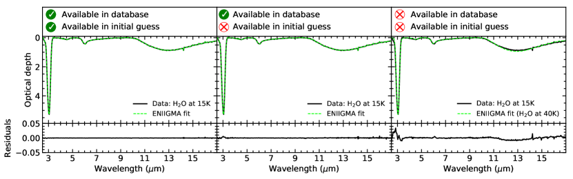
Figure 3: ENIIGMA fit (dashed green line) of the pure H₂O ice sample at 15 K (black line). Left and middle panels show the fit in fully sighted and blinded tests, respectively. The right panel shows the fit when the correct solution does not exist. The residuals of the fit are shown in the boxes below the fits.

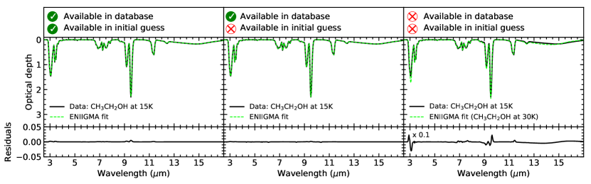
Figure 4: Same as Figure 3, but for pure CH₃CH₂OH at 15 K.

Binary ice mixture: A mixture dominated by H₂O (95%) ice containing a fraction of ethanol (5%) at 15 K is used in the test with binary ice sample. Despite the small fraction, ethanol shows clearly features around 9 $\mu$m and 11 $\mu$m. The fitting results are shown in Figure 5. The left and middle panels showing the fully sighted and fully blinded tests indicate that the correct ice spectra were assigned with residuals lower than 5%. In the case where the correct solution is not available (right panel), the H₂O:CH₃CH₂OH at 30 K was selected by the fitting routine. As in the pure ice case, this fit indicates that the ENIIGMA tool is able to select the most similar ice sample to fit the input spectrum. Because of the small differences of this ice mixture at 15 K and 30 K, the residual is around 5%.

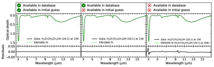
Figure 5: Same as Figure 3, but for H₂O:CH₃CH₂OH (20:1) at 15 K.

Ternary ice mixture: The third test is performed with a tertiary ice mixture composed by CO:CH₃OH:CH₃CH₂OH (20:20:1). As seen in Figure 6, the fits were also accurate for the fully sighted and blinded tests (left and right panels). The residual in the middle panel is higher than in the left panel, clearly showing the random nature of the method. The fit in the right panel was performed by combining two ice samples, namely, CO:CH₃CH₂OH at 30 K and CH₃CH₂OH at 30 K. Because of the prominent CO feature in the input spectrum, not present in the ethanol ice, the code combined the two samples in order to provide a good fit. The reason why the pure CO ice was not used in this fit is that its full width half maximum is 30% narrower than in the mixture with ethanol.

Figure 6: Same as Figure 3, but for CO:CH₃OH:CH₃CH₂OH (20:20:1) at 15 K.

Quaternary ice mixture: The final test about the identification of known samples is performed with H₂O:CH₃OH:CO:NH₃ (100:50:1:1) at 10 K, where both water and methanol features are prominent. Left and middle panels of Figure 7 show the result in the fully sighted and blinded tests, respectively. Again, the fits result in residuals lower than 5%. Slightly higher residual are seen in the right panel, where the solution is not available in the database. In that case, the ice sample composed by the sample molecules at 40 K was provided with the fit. As in the case of the tertiary mixture, this result indicates that a combination of the pure molecules does not result in a good fit. For example, Dawes et al. (2016) show that the peak position of the O$-$H vibrational at around 3.0 $\mu$m is redshifted in a mixture of H₂O:CH₃OH compared to the pure H₂O. Nevertheless, the temperature difference of this mixture at 10 and 40 K is evident by the residuals. At this temperature, most of the CO ice has been thermal desorbed (Collings et al., 2004; Acharyya et al., 2007), whereas a small fraction trapped in the ice porous has enough energy to migrate over active sites.

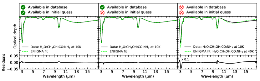
Figure 7: Same as Figure 3, but for H₂O:CO:NH₃:CH₃OH at 10 K.

3.2 Fractionation

As water represents the major component of astrophysical ices observed toward YSOs, this section aims to check the capability of the ENIIGMA tool in finding the correct coefficients in a linear combination of H₂O ice and another component. In the tests shown in Sections 3.2.1-3.2.3, two IR ice spectra were summed with different coefficients and Gaussian noise of standard deviation equal to 0.01 has been added to the data to resemble the noise present in the astronomical observations. Although the tests in Sections 3.2.1 and  3.2.2 use water ice spectra at two different temperatures, the aim is to discuss the fractionation of constructed mixtures with similar spectral bands, rather than thermal processing. The searching Methods 1$-$3 in Table 2 provided the expected global minimum solutions. In the test shown in Section 3.2.5, eight IR ice spectrum were considered to mimic the ice absorption features observed toward protostars. In this case, only Methods 2 and 3 provided the best fits.

3.2.1 H₂O (15K) and H₂O (40K)

IR spectra of pure water at 15 K and 40 K were summed with proportions of 50:50 and 90:10, respectively. These two ice data were selected because they have small differences in the band shapes and thus represents a challenging task for fitting methods. Figure 8 shows the test results for these two H₂O ice spectra. The top left panel shows the good match between the ENIIGMA fit and combined H₂O ice data with proportions of 50:50. The residual plot in the bottom part of this figure shows that only the Gaussian residual noise is left after subtracting the model from data. The top right panel shows a $\Delta\chi^{2}$ map, where the confidence intervals (1$-$3$\sigma$) are indicated by the green, yellow and red contours, respectively. As one can note in this degeneracy analysis, the increasing of the H₂O proportion at 15 K with simultaneous decreasing of the proportion of H₂O at (40 K) also provides statistically significant results inside the confidence intervals.

The two bottom panels of Figure 8 shows the same test for the proportion of 90:10 at 15 K and 40 K, respectively. The spectral decomposition is shown in the left panel also shows a good match between the ENIIGMA fit and the combined H₂O ice data, with residuals lower than 5%. In this test, the $\Delta\chi^{2}$ map shown in the right panel indicates that a solution considering only H₂O (15 K) is also statistically possible when the fraction of H₂O (40 K) is lower than 10%. The same solution is still found by the ENIIGMA tool with the $\sigma_{\rm{noise}}$ equal to 0.02. Above that limit, the ENIIGMA is unable to find the H₂O (40 K) component.

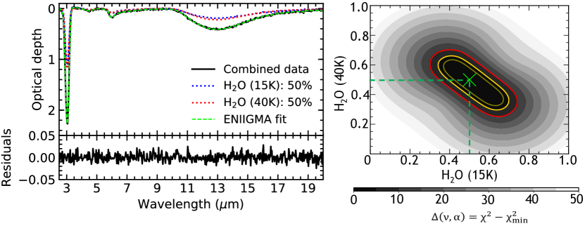
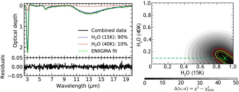
Figure 8: Spectral decomposition and confidence interval analysis of the ENIIGMA results. Left panels show the spectral decomposition of the combined water ice spectra (black solid line) with proportions of 50:50 and 90:10. The components of the decomposition are given by the red and blue dotted lines, whereas the ENIIGMA fit is given by the green dashed line. The residual of the fit is shown in the bottom parts of these graphs. Right panels show the confidence interval analysis of the coefficients in the linear combination. The greyscale colours are the difference between chi-square and minimum chi-square values; the olive, yellow and red contours are 1$\sigma$, 2$\sigma$ and 3$\sigma$ confidence intervals, respectively.

For the case where the H₂O ice proportions are 90:10, a population evolution analysis is shown in Figure 9. At the initial generations, most of the population values result in high fitness score (white region) and therefore the optimal coefficients have not been found yet. As the optimization evolves, the population is improved and better coefficients are generated because of the survival of the best solution. Close to generation 85, most of the population results is low fitness score, which increases the probability of finding the global minimum solution of the problem. The fitness score evolution over the generations is shown in the bottom panel of Figure 9. As noted in the top panel, the fitness score at the initial generations is high for any value in the population. With the improvement of the population, the fit is improved until finding the optimal solution between generations 80 and 85, with $\chi_{\nu}^{2}=1.01$. As the population has not converged in this problem, the fitness score starts increasing again until generation 100, which is the stopping criteria in this problem.

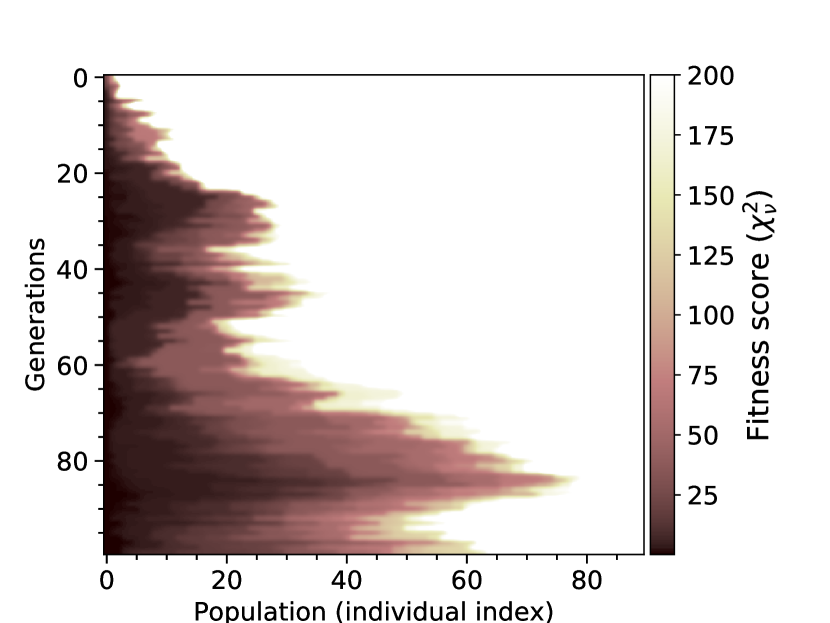
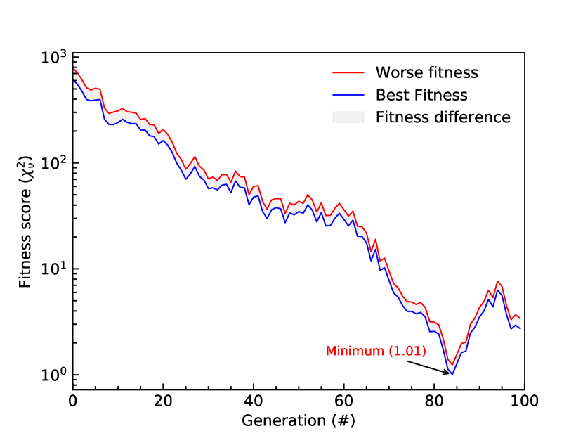
Figure 9: Top: Heat map of the fitness score for each population over the generations. Bottom: Fitness score over the generations. The blue and red colours indicate the best and worse fitness based on the population of each generation. The grey shaded area between the two lines shows the difference between the worse and best fitness.

3.2.2 H₂O (15 K) and H₂O (75 K)

A second check with water ice samples at (15 K) and (75 K) was also made. At high temperatures the water band shapes are significantly different than in the cases of 15 K and 40 K because of the transition from amorphous to cubic crystalline ice (Hudgins et al., 1993). In particular, the O$-$H band at 3 $\mu$m is gradually sharpened until the full crystalline ice is formed between 100$-$140 K (Sack & Baragiola, 1993). As shown in the left panels of Figure 10, the ENIIGMA tool is able to identify the correct proportions of the two samples in the cases of 50:50 and 10:90, respectively. This is also indicated by the low fit residuals around 5% in both situations.

The confidence intervals of the optimal solution are shown in the right panels of Figure 10. In these plots, the reduced area of the contours compared to Figure 8 indicates that the solution is less degenerated. The reason is the differences of the band shapes of the cold and warm H₂O ice components. In the case of 50:50 proportion shown in the top right panel, the 3$\sigma$ confidence interval of both coefficients is around 20%. On the other hand, in the bottom right panel, the degeneracy of the 10:90 proportion is 50% and 10%, respectively, which indicates that the H₂O (75 K) component is better constrained than the H₂O (15 K) component.

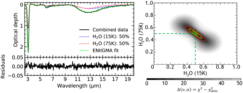
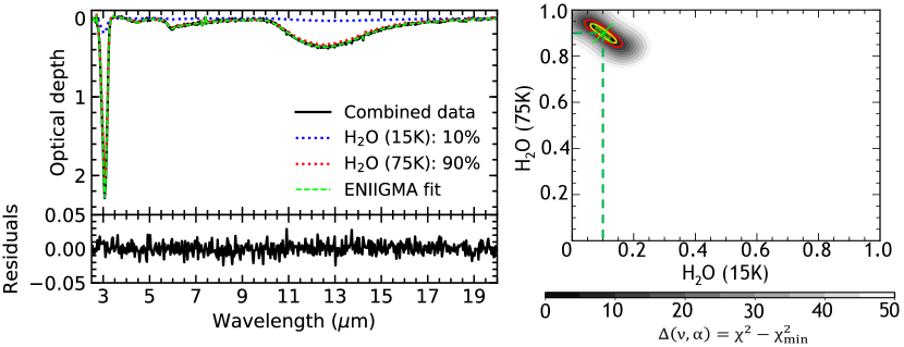
Figure 10: Same as Figure 8, but for H₂O at 15 K and 75 K.

After the global minimum solution is found, the degeneracy analysis of the ice composition is performed for the case with proportions of 10:90. Figures 11a-c show the IR spectra of H₂O ice at 15, 40 and 75 K. As one can note, the spectral shape of the bands is similar between the samples at 15 and 40 K, and significantly different at 75 K because of the crystallization of the ice matrix via warm-up. An initial test has been done with the sum of the two H₂O ice samples at 15 and 75 K without Gaussian noise and the recurrence plot was created. The recurrence plot shown in panel d indicates that no degeneracy exists inside 3$\sigma$ confidence interval when the spectrum is absent of noise. On the other hand, if Gaussian noise is added to the summed spectrum, the degeneracy becomes evident. The dominant ice component, H₂O at 75 K is still present in all solutions inside the same confidence interval, whereas the recurrence of water component at 15 K is reduced to 50% because of its lower contribution. The presence of other samples in this recurrence analysis indicate that the H₂O (15 K) can be replaced by one of those data, and still provide good solution inside 3$\sigma$ confidence interval.

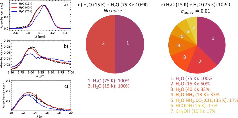
Figure 11: Degeneracy analysis for the combination of H₂O (15 K) + H₂O (75 K): 10:90. Panels a.$-$c. show respective stretching, bending and librational modes of H₂O ice at 15, 40 and 75 K. These panels highlight the temperature effect on the band shapes in the water ice IR spectra. Panel d shows the recurrence pie chart for the fit of the combined data H₂O(15 K):H₂O(75 K) with proportions 10:90, respectively and without adding Gaussian noise to the spectrum. Panel e shows the same as Panel d, but after adding Gaussian noise to the spectrum ($\sigma=0.01$).

3.2.3 H₂O (15K) and CO:CH₃OH:CH₃CH₂OH (15K)

In this test, the combination of H₂O and the mixture CO:CH₃OH:CH₃CH₂OH (20:20:1) at 15 K is used. In general, these two ice data have different band peaks and shapes in the IR spectrum, although the O$-$H stretching modes of H₂O and CH₃OH overlaps around 3 $\mu$m. Another difference is that the samples do not have the same ice thickness. Figure 12 shows the fits of the proportion 50:50. Because of the thickness difference, the water ice has a major contribution to the band at 3 $\mu$m compared to methanol, whereas at 4.67 $\mu$m and 8.86 $\mu$m the presence of the mixture sample becomes evident. The residuals of the fit are lower than 5% and indicate a good match between fit and combined data. The confidence interval analysis of the coefficients, shown in the top right panel indicates that the water and mixture components vary in about 20% and 40%, respectively, inside 3$\sigma$.

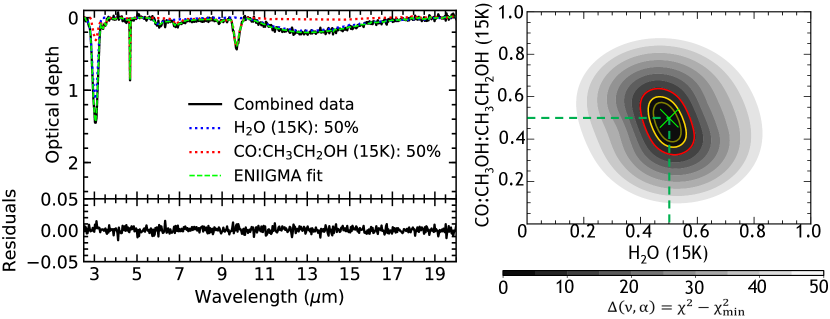
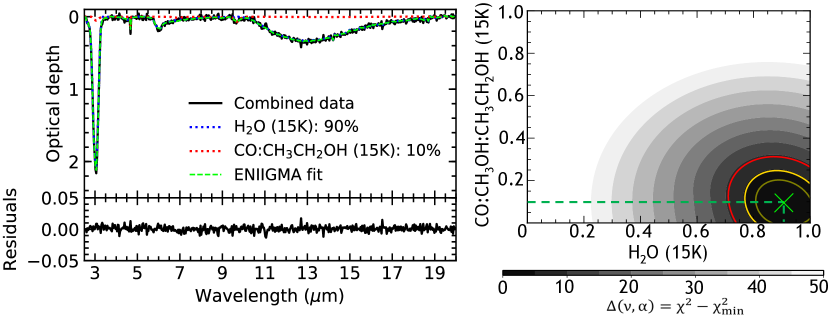
Figure 12: Same as Figure 8, but for H₂O and CO:CH₃CH₂OH at 15 K.

The bottom left panel shows the fit of the proportions 90:10 for the water and mixture samples, respectively. In this case, the contribution of methanol at 3 $\mu$m is minimal, although it still visible around 9 $\mu$m. As seen from the residuals of the fit, the decomposition process was also able to identify the correct coefficients of the two samples. However, because of the small contribution of the mixture, the confidence interval analysis (bottom right panel) indicate that solutions considering only pure water are statistically significant as well.

3.2.4 Spurious features

To test the effect of spurious bands that could be present in a real observational spectrum, we added emission and absorption features of non-ice compounds to the constructed mixture shown in Section 3.2.3. The emission features mimic the hydrogen lines at 3.04 $\mu$m (HI Pf$\epsilon$ 5$-$10), 3.30 $\mu$m (HI Pf$\delta$ 5$-$9), and 3.74 $\mu$m (HI Pf$\gamma$ 5$-$8). These lines are seen in spectra observed with ground-based telescopes when the standard star is not properly modelled (e.g., Pontoppidan et al., 2004; Thi et al., 2006). These emission profiles were created with the Python package pysynphot (STScI Development Team, 2013) by adopting full width at half maximum of 50 $\AA$. For the absorption feature, we use the naphthalene (C₁₀H₈) spectrum taken from Hudgins & Sandford (1998), that is the simplest polycyclic aromatic hydrocarbon containing two rings. Naphthalene has multiple bands between 3.20 $\mu$m and 3.44 $\mu$m, where features of methanol and ethanol are also present.

Figure 13 displays the spectral decomposition of a constructed mixture containing ice bands (H₂O and CO:CH₃OH:CH₃CH₂OH) and spurious features. Once these emission and absorption features are located shortwards of 4 $\mu$m, the ENIIGMA fit is performed between 2.5 $\mu$m and 4.0 $\mu$m. This test shows that the ENIIGMA fitting tool identify correctly the ice bands and does fit the narrow features associated with spurious absorption and emission lines. In this example, the spectral profile between 3.2 $\mu$m and 3.5 $\mu$m is the most affected with spurious features, but those features do not change the shape of the ice bands. We highlight that in real observations, other spurious features might occur in the spectrum due to poorly continuum subtraction, as well as the effect of spectral glitches and baseline jumps. In these cases, a broad band fit of the spectrum covering other vibrational modes of the same molecule could minimize the effect of spurious features in the spectral decomposition with the ENIIGMA package.

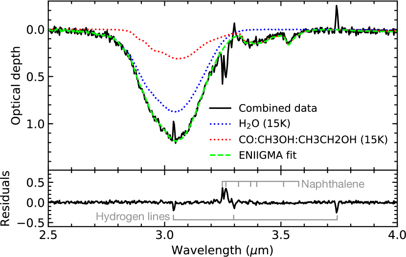
Figure 13: Spectral decomposition of the H₂O and CO:CH₃OH:CH₃CH₂OH constructed mixture containing spurious features mimicked with hydrogen lines and naphthalene bands.

3.2.5 Synthetic ice spectrum

Multiple ice features have been observed in the IR spectra of protostars (e.g., Gibb et al., 2004; Zasowski et al., 2009). For example, a linear combination of five empirical components, which are associated to more than one carrier, have been adopted to decompose the short spectral range between 5$-$8 $\mu$m (Boogert et al., 2008). In this test, a synthetic ice spectrum is created based on the median ice composition derived by Öberg et al. (2011) towards low-mass protostars, namely, H₂O:CO:CO₂:CH₃OH:NH₃:CH₄:XCN (1:0.29:0.29:0.03:0.05:0.05:0.003). However, the chemical specie XCN is replaced by 2% of CH₃CHO and 1% of CH₃CH₂OH with respect to the water ice to check the feasibility to identify these molecules with the ENIIGMA tool. The synthetic spectrum, shown in Figure 14a, is created with the linear combination of IR spectra of eight pure ices (temperatures: 10$-$15 K) listed in Table 4 and the silicate spectrum from GCS 3 taken from Kemper et al. (2004). Also, a Gaussian noise of $\sigma$ equal to 0.01 is added to the spectrum. This highlights that a real spectrum might have such a strong silicate features, and that they must be subtracted off before the the spectral decomposition with the ENIIGMA tool. The procedure of silicate removal in an observed spectrum is shown in Sections 2.2 and 4.1.

The initial guess adopted in this test is made of H₂O (40 K), NH₃ (10 K) and CH₃OH (75 K). Figures 14b$-$e show the result of the spectral decomposition. Although the expected global minimum solution was found by the three methods in Table 2, Method 1 provided less accurate coefficients in about 4$-$7%. In the top panel, the fit is shown for the range between 2.5$-$20 $\mu$m. At this scale, only the major features are seen, such as H₂O (3 $\mu$m, 6 $\mu$m, 13 $\mu$m), CO₂ (4.27 $\mu$m, 15.53 $\mu$m), CO (4.67 $\mu$m) and CH₄ (7.673 $\mu$m). The residual plot shows that only the Gaussian noise is left after subtracting the data from the model, which indicates that both the samples and the coefficients were found by the ENIIGMA fitting tool. The bottom panels show a zoom-in of the regions where the weak features are detected. The left panel highlights the C$-$H stretching mode at 3.53 $\mu$m. The middle panel shows the contribution of CH₃CHO at 5.8 $\mu$m, and 7.4 $\mu$m, NH₃ at 6.2 $\mu$m and CH₃OH at 6.8 $\mu$m. The right panel shows the dominant absorption features of NH₃ at 9.35 $\mu$m and CH₃OH at 9.8 $\mu$m, with small contributions of CH₃CHO at 8.9 $\mu$m and the CH₃CH₂OH double peaks at 9.2 $\mu$m and 9.5 $\mu$m.

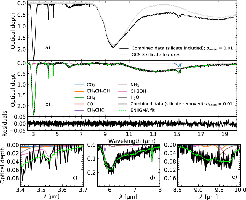
Figure 14: Spectral decomposition of the synthetic ice spectrum composed of 8 components of pure ice sample (black line) and Gaussian noise ($\sigma=0.01$). Panel a shows the synthetic spectrum along with the silicate band from 2.5$-$20 $\mu$m. Panel b displays the synthetic spectrum without the silicate feature and residual plot.

The ENIIGMA fit is shown by the dashed green line and the ice components by the other colours. Panels c-e show small spectral ranges highlighting the contribution of shallow bands.

In summary, these tests show that the ENIIGMA can find the correct components and linear combination coefficients in the combined spectral data. However, Methods 2 and 3 provides better results than Method 1 when the number of components is large.

4 Application to infrared spectra of the Class I protostar Elias 29

To test the ENIIGMA fitting tool with a real source, an spectral analysis of the well-known Class I YSO, Elias 29 is carried out. This object is located in the Ophiuchus cloud, at an estimated distance of 135 pc (Ortiz-León et al., 2018). Elias 29 is the brightest source in the $\rho$ Oph E core and was observed in broad IR spectral range by the Infrared Space Observatory. Multiple absorption bands were securely and tentative detected in the IR spectrum of this protostar (Gibb et al., 2004; Boogert et al., 2000; Rocha & Pilling, 2015). Millimeter observations toward Elias 29 show high abundances of simple molecules (e.g., CO, H₂CO, HCO⁺, SO, SO₂; Boogert et al., 2002; Oya et al., 2019) and deficiency of complex molecules (e.g., CH₃OH, HCOOCH₃, CH₃OCH₃; Artur de la Villarmois et al., 2019; Oya et al., 2019). In particular, Oya et al. (2019) attribute the lack of organic molecules and richness in SO and SO₂ to the evolved nature of the source or the enhancement of the dust temperature above the CO freeze-out regime ($>$ 20 K) as suggested by Rocha & Pilling (2018) based on radiative transfer models. Artur de la Villarmois et al. (2019) suggest that the non-detection of warm CH₃OH toward Elias 29 and other sources in Ophiuchus molecular cloud, is due to the absence of hot-core like region in the inner envelope close to the protostar or the due to higher temperatures in the precursor environments, as also discussed in the case of Corona Australis (Lindberg et al., 2014).

4.1 Continuum and optical depth calculation, and silicate feature extraction

In this paper, the continuum SED of Elias 29 has been determined with a blackbody function shortwards of 4.2 $\mu$m and a low-order polynomial function between 4.1 $\mu$m and 30 $\mu$m. In the former case, the spectrum between the ranges 2.5$-$2.8 $\mu$m and 3.9$-$4.2 $\mu$m are absent of ice features and thus were used to constrain the fitting. In this case, a temperature of 717 K provided the best match with the observations. Longwards of 4.1 $\mu$m, a third-order polynomial fitting passing through spectral ranges without ice features (4.1$-$4.25 $\mu$m, 4.3$-$4.5 $\mu$m, 5.3$-$5.5 $\mu$m and 25$-$30 $\mu$m) has been adopted. Pontoppidan et al. (2005) mention that although this method has some uncertainty involved, the shape of the bands are not affected even though the total optical depth is uncertain by up to 20%. The top panel of Figure 15 shows the result of this fit and other calculations in the literature. The fits from Boogert et al. (2000) and Rocha & Pilling (2015) agrees better with the continuum SED calculated in this paper, whereas the fit from Boogert et al. (2002) mismatch the observations.

Once the continuum SED is determined, the observational optical depth is calculated with Equation 3, and the result is shown in the middle panel of Figure 15. The continuum methods used in this paper and Boogert et al. (2000) results in similar optical depths. The differences between the two methods are shown in the bottom panel of Figure 15 and are less than 10% in the range between 2.5$-$30 $\mu$m. A similar variation is reported by van Breemen et al. (2011) for the band at 9.8 $\mu$m, when different continuum models are assumed for the objects StRs 164 and SSTc2d_J163346.2$-$242753. Most importantly, they concluded that the shape of the 9.8 $\mu$m bands remains virtually unaffected, which is in agreement with the result shown in this work. On the other hand, the effect of alterations in the shape of the silicate band at 18 $\mu$m are much less constrained.

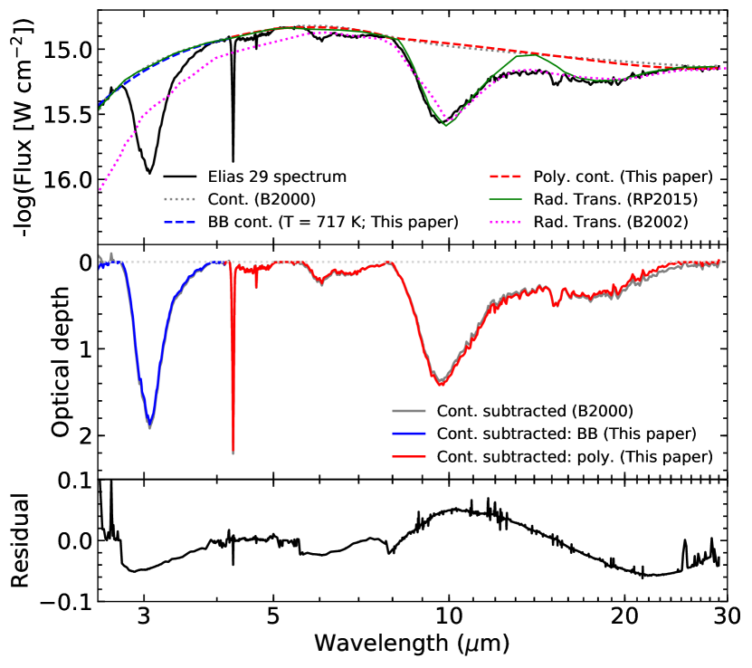
Figure 15: Continuum determination and optical depth calculation of the Elias 29 spectrum. Top: Blue and red dashed lines show, respectively, the blackbody and polynomial continuum calculation used in this paper. The grey dotted line shows the continuum determination from Boogert et al. (2000), which is similar to the continuum in this paper. The dotted magenta line is the continuum calculation with radiative transfer modelling from Boogert et al. (2002). The green solid line is the continuum calculation with radiative transfer modelling from Rocha & Pilling (2015). In both cases, the silicate feature is red-shifted in the models compared with the observations. Middle: Grey line shows the optical depth scale of Elias 29 spectrum adopting the continuum from Boogert et al. (2000), whereas blue and red lines show the same by respectively adopting blackbody and polynomial continuum derived in this paper. Bottom: Difference in optical depth estimates from this paper and Boogert et al. (2000).

The silicate absorption in the spectrum of Elias 29 is removed following the procedure described in Section 2.2. It is observed in the top panel of Figure 16 that the GCS 3 silicate feature resembles well the absorption band seen toward Elias 29, suggesting they could have similar mineralogy. In this particular case, the modification of the 9.7 $\mu$m band shape is minimal as can be noted in the result of the silicate extraction in the bottom panel of Figure 16. The major difference in the two methods is only the absorption excess at 8.8 $\mu$m, previously discussed in Section 2.2. With the synthetic silicate band, this leftover residual is subtracted off. Figure 16a also shows an absorption excess between 11$-$18 $\mu$m between the broad silicate bands at 9.8 $\mu$m and 18 $\mu$m that is clearly seen in the silicate feature subtracted spectrum (Figure 16b.) Because of the uncertainties in the continuum and in the silicate band profile at 18 $\mu$m, some effect could be added to this band with silicate subtraction. However, Boogert et al. (2008) and Zasowski et al. (2009) convincingly shows that this entire feature is associated with the H₂O ice libration mode.

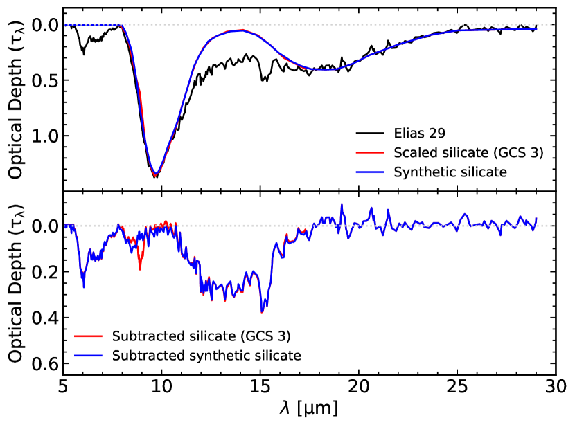
Figure 16: Silicate extraction procedure in the Elias 29 spectrum. Top: Black line shows the optical depth scale of the Elias 29 spectrum calculated in this paper. Red and blue lines show, respectively, the scaled CGS 3 and synthetic silicate bands at 9.7 $\mu$m and 18 $\mu$m. Bottom: Red and blues lines show the Elias 29 mid-IR optical depth after silicate band extractions with scaled CGS 3 and synthetic silicate profiles, respectively.

4.2 Spectral decomposition

The Methods 1$-$3 in Table 2 were used to decompose the IR spectrum of Elias 29. The initial guess adopted in this study is composed of the pure ice samples H₂O, CO, CO₂ and NH₃. After selecting the best candidates for the solution, the entire sample is combined in groups of 7 components. The best global minimum was found in Method 3, and the result is shown in Figure 17a$-$f. In Panel a, the spectral decomposition in the range between 2.5$-$20 $\mu$m highlights the fitting of the most prominent bands, whereas the Panels b$-$f bottom panels show zoom-in of small spectral ranges and the contributions of shallow features. The spectral features of a$-$C(:H), taken from Alata et al. (2014), are also shown in these panels to illustrate potential contributions of carbonaceous grains as discussed by Jones (2012, 2016).

The global minimum solution in the Elias 29 spectral analysis is given by the combination of pure and mixed ice samples. The dominant component in this broadband analysis is H₂O:NH₃:CO₂:CH₄ (10:1:1:1) at 35 K and processed by heavy ions, simulating the effects of cosmic rays. This sample has significant contributions at 3 $\mu$m, 6 $\mu$m and 11$-$18 $\mu$m and 15 $\mu$m. The second prominent component is CO₂ with vibrational modes at 4.27 $\mu$m and 15 $\mu$m. Pure and mixed H₂O components also contribute about 20% of the remaining absorption at 3 $\mu$m. The shallow features observed in this spectral decomposition are CO, NH₃, CH₄, CH₃CH₂OH.

An old-standing problem in the analysis of mid-IR spectra of YSOs and background sources is that the band at 6 $\mu$m is deeper than what is expected from the 3 $\mu$m and 13 $\mu$m H₂O ice bands (e.g., Cox, 1989; Gibb et al., 2000; Boogert et al., 2008; Bottinelli et al., 2010; Boogert et al., 2011). A potential explanation for the absorption excess at 6 $\mu$m is the presence of organic refractory material (Gibb & Whittet, 2002), although it lacks independent spectroscopic confirmation (Boogert et al., 2015). Another open question in this context is the correct carrier of the band at 6.85 $\mu$m. Although the most likely candidate is NH${}_{4}^{+}$ (Schutte & Khanna, 2003), it lacks a convincing profile fit as pointed-out by Boogert et al. (2015).

In this paper, the global optimization with the ENIIGMA tool provided a good fit of the absorption bands observed in the Elias 29 spectrum between 2.5$-$20 $\mu$m. The feature at 3 $\mu$m associated with the O$-$H vibrational mode is fitted by multiple ice sample containing water. However, there is an absorption excess in the Elias 29 spectrum that is not fitted with the ice samples in this case (Figure 17b). One of the explanations for this excess is the absorption caused by ammonia hydrates (e.g., Knacke et al., 1982; Dartois & d’Hendecourt, 2001). Another cause is attributed to the light scattering due to large grains (Smith et al., 1989). Jones (2016) also suggest that compounds containing the carbonyl functional group (C$=$O) present in the dust before or during the formation of the ice mantle, could be a potential explanation for this absorption excess. Figure 17b shows that a$-$C(:H) could contribute to the large absorption excess around 3.5 $\mu$m, although the absorption features at 6.85 $\mu$m and 7.24 $\mu$m lacks visual matching with the observations (Figure 17e). Because of the low spectral resolution, this does not disregard the presence of a small fraction of a$-$C(:H) in the dust grains toward Elias 29. However, Boogert et al. (2000) argue that for the case of Elias 29, the scattered light due to large grains is the likely explanation because of the good matching of this red wing obtained with large icy grains.

The CO₂ stretching component at 4.27 $\mu$m (Figure 17c) is found to be a combination of pure and mixed CO₂. However, the peak optical depth in the fit does not match with the observations because it is also constrained by the CO₂ bending mode at 15.1 $\mu$m. Adding more CO₂ to the feature at 4.27 $\mu$m would lead to absorption excess at 15.1 $\mu$m. On the other hand, the CO ice band at 4.67 $\mu$m (Figure 17d) is reproduced in this study by three components, namely, pure CO ice, CO:CH₃OH and CO formed with the cosmic-ray processing of H₂O:NH₃:CO₂:CH₄ (10:1:1:1) at 35 K, which is in agreement with the literature. Previous studies of the structure of CO ice band (e.g., Pontoppidan et al., 2003a; Thi et al., 2006; Perotti et al., 2020), have shown that this band is well fitted by three Gaussian components or a combination of laboratory data and analytical functions. Such components are associated with pure CO, and CO mixed in polar ice matrices (e.g., H₂O and CH₃OH; Cuppen et al., 2011).

The broadband between 5.5$-$8.0 $\mu$m (Figure 17e) is well fitted by combining multiple components. In particular, two ice samples processed by UV (H₂O:NH₃:CH₃OH:CO:CO₂; Muñoz Caro & Schutte, 2003) and cosmic rays (H₂O:NH₃:CO₂:CH₄ Pilling et al., 2010) significantly contribute to fit the Elias 29 spectrum. The ammonium ion (NH${}_{4}^{+}$) is a common byproduct of the ice processing in these two cases, and is one of the proposed carriers of the band at 6.85 $\mu$m. The significant contribution of these two IR ice spectrum might indicate that the chemical evolution of Elias 29 is mostly induced by energetic processing of the ice mantles.

In the presented spectral analysis, CH₃CH₂OH mixed in H₂O ice is a likely carrier of absorption bands at 7.5 $\mu$m and 9.6 $\mu$m (Figure 17e,f). Although the ethanol bands cannot be resolved at 7.5 $\mu$m with ISO observations, the band at 9.6 $\mu$m could indicate a tentative detection of this complex organic molecule toward Elias 29. This result also shows the contribution of methanol ice at 9.75 $\mu$m. Most importantly, this result shows that the band between 9.5$-$10 $\mu$m might not be only associated with methanol as suggested previously (e.g., Boogert et al., 2008; Bottinelli et al., 2010), but rather that it is due to the presence of other alcohols in ices as discussed by Jones (2016). Consequently, the reduced amount of methanol in ices would contribute to partially solve the conundrum of the low gas-to-ice ratio observed toward star-forming regions ($\sim$ 10^-4; Öberg et al., 2009; Perotti et al., 2020, 2021), as also conjectured by Jones (2016). However, we stress that high resolution spectral data are required to unambiguously detect complex molecules in ices beyond methanol.

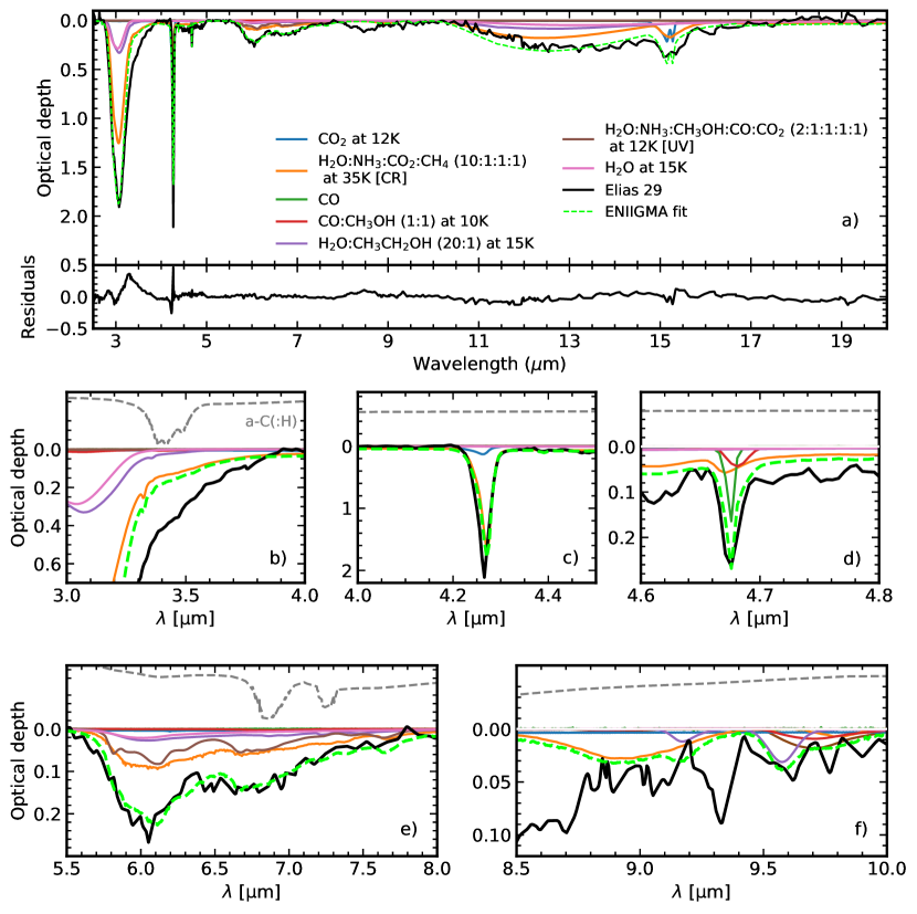
Figure 17: Spectral decomposition of the mid-IR spectrum of Elias 29 protostar. a): Optical depth scale of the observed spectrum between 2.5$-$20 $\mu$m, and the seven ice components used to fit the observed spectrum. The best fit is shown by the dashed green line. The residual spectrum is shown below this panel. b-f: Zoom-in of short spectral ranges highlighting the contribution of small features. In these plots, the spectral features of amorphous carbon, a-C(:H), that were not used in the spectral decomposition, are shown by the dashed grey lines above the Elias 29 spectrum and the ice data components. This illustrates potential contribution of features other than vibrational modes of ice species.

Panel b shows the L-band red wing absorption excess that is not entirely reproduced by the ice components (see Section 4.2). Panels c and d display the CO₂ and CO features. Panel e shows important contributions of UV and cosmic-ray processed samples. Finally, Panel f highlights the contribution of the broad NH₃ ice feature at 9 $\mu$m, CH₃CH₂OH at 9.6 $\mu$m and CH₃OH at 9.8 $\mu$m.

4.3 Recurrence analysis of the spectral decomposition

Because the ice spectral features vary with the physical and chemical environment such as composition, temperature, and radiation field, the fits of observational IR spectra of YSOs are often degenerate. The recurrence pie chart (Section 2.7) is used to verify uniqueness of the solution found with the ENIIGMA and the result is displayed in Figure 18.

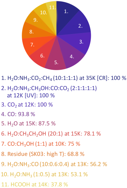
Figure 18: Recurrence pie chart of the IR ice data contributing to solutions inside 3$\sigma$ confidence interval ($\Delta\chi^{2}\leq 18.5$). The size of each piece is proportional to the contribution of each sample.

This analysis shows that the samples 1$-$7 have recurrence above 75%, and are also the components providing the global minimum solution as seen in Figure 17. The samples 1$-$3 have a recurrence of 100%, and thus are solutions that cannot be replaced. Additionally, they have a significant contribution to the strong absorption features in the Elias 29 spectrum. The CO sample has a recurrence of 93.8% since the C-O stretching mode at 4.67 $\mu$m can be combined with other solutions containing CO, such as sample 1 (CO formed after processing; see Section 4.2) and samples 7 and 9. The recurrence of pure H₂O (87.5%) indicates that this component is necessary for the global minimum solution, but not crucial. Other samples containing H₂O (e.g., 6, 9 and 10), can also be adopted to provide a good fit of the water absorption bands. Sample 6, is the only component containing CH₃CH₂OH. However, because this sample is dominated by water ice, that can be replaced by another component, its recurrence is 78.1%. Sample 7 has a recurrence of 75% and is important to fit the red wing of the absorption band at 4.67 $\mu$m.

The samples 8$-$11 are less recurrent (37.7$-$68.8%), although still inside the 3$\sigma$ confidence interval. In particular, sample 8 contains a strong NH${}_{4}^{+}$ feature that could replace component 2 in the fits. However, it is not part of the global minimum solution because the bandwidth at 6.85 $\mu$m of component 8 is lower than in component 2, which provided a good match with the observational spectrum. In the cases of samples 9 and 10, they provide less accurate fit compared to components 1, 5, and 6. The less recurrent component, HCOOH, has been tentatively detected towards Elias 29. Despite formic acid is not part of the global minimum solution, it is not excluded as a potential carrier to fit the Elias 29 spectrum.

4.4 Ice column density

Ice bands can be blended in the IR spectrum, and thus the selection of clear absorption features is essential to provide accurate quantification of the ice column densities. With the spectral decomposition used in this paper, the bands associated with different molecules were isolated, and their ice column densities calculated using Equation 9 and the band strengths listed in Table 1. The derived values are shown in Table 3 and are compared with previous calculations by Boogert et al. (2000). The lower and upper bounds are calculated from the 3$\sigma$ confidence interval analysis shown in Figure 19. Table 3 also shows the median ice column densities calculated from the histograms shown in Appendix B. These values take into account all solutions found by the ENIIGMA tool inside 3$\sigma$ confidence interval.

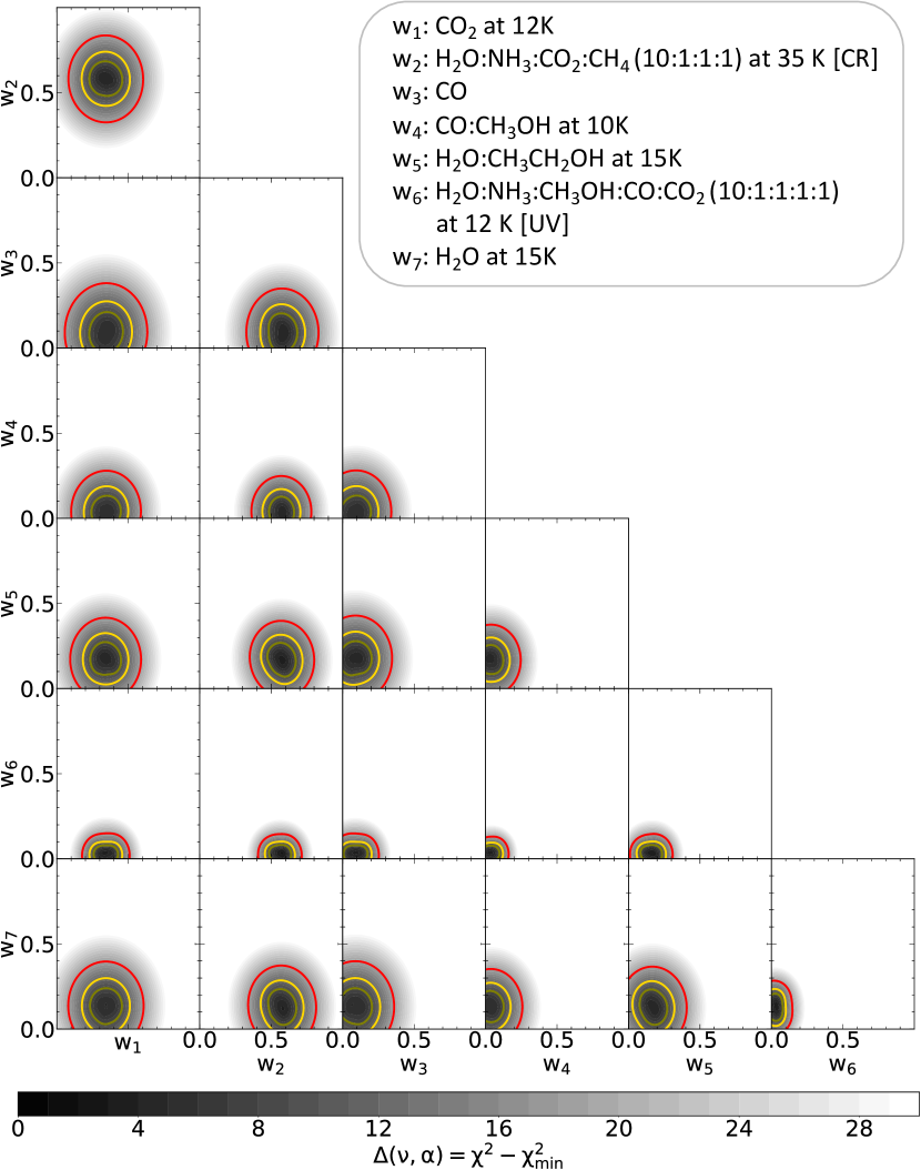
Figure 19: 2D $\Delta\chi^{2}$ maps in grey-scale showing the correlation between seven ice laboratory data used to decompose the Elias 29 spectrum. The green, yellow and red contours indicate 1$-$3$\sigma$ confidence intervals, respectively. For seven components, they are defined for $\Delta\chi^{2}$ equal to 8.38, 12.02 and 18.48.

Table 3: Ice column densities towards Elias 29. Tentative detection in the literature are shown as 3$\sigma$ upper limit and non-detection as “NA”.

Specie	$N_{\rm{ice}}$ [$10^{17}$ cm-2]	This paper: $N_{\rm{ice}}$ [$10^{17}$ cm-2]
	Boogert et al. (2000)	Global minimum	Median (Histogramb)
H2O	34 (6)	33.11${}_{21.09}^{41.13}$	35.42${}_{25.23}^{41.87}$
NH3	¡ 3.5	1.01${}_{0.75}^{1.47}$	2.42${}_{0.43}^{3.88}$
CO	1.7 (0.3)	1.55${}_{0.73}^{1.81}$	1.42${}_{1.23}^{1.87}$
CO2	6.7 (0.5)	5.22${}_{3.4}^{7.13}$	4.42${}_{2.23}^{6.87}$
CH4	¡ 0.5	0.38${}_{0.17}^{0.51}$	0.42${}_{0.02}^{1.12}$
H2CO	¡ 0.6	0.38${}_{0.13}^{0.42}$	0.27${}_{0.03}^{0.52}$
CH3OH	¡ 1.5	0.86${}_{0.06}^{1.16}$	1.70${}_{0.21}^{2.38}$
CH3CH2OH	NA	0.08${}_{0.03}^{0.11}$	0.12${}_{0.02}^{0.40}$
NH${}_{4}^{+}$	1.01 (0.3)a	1.15${}_{0.3}^{0.72}$	1.02${}_{0.23}^{3.12}$
HCOOH	¡ 0.3	NA	0.55${}_{0.13}^{0.91}$
OCS	¡ 0.015	NA	NA
OCN-	¡ 0.067	NA	NA

Water ice has multiple bands detected in the Elias 29 spectrum. In this paper, the water libration mode at 14 $\mu$m is used in the calculation as it easily separated from the CO₂ vibrational mode at 15 $\mu$m. The bands at 3 $\mu$m and 6 $\mu$m are blended with strong features of some molecules such as CH₃OH, HCOOH and processed ice, which makes difficult the correct extraction of the water band. In the cases of CO₂ and CO, the respective bands at 4.27 $\mu$m and 4.67 $\mu$m were used to derive the column densities. However, the pure and mixed CO₂ components found in the decomposition were not sufficient to reproduce the observed absorption band, and the $N_{\rm{CO_{2}}}$ ice column density in this paper is 28% lower than found by Boogert et al. (2000). On the other hand, the $N_{\rm{CO}}$ values match well within the uncertainties. The ice column densities of calculated in this paper for H₂CO (5.83 $\mu$m), CH₃OH (6.83 $\mu$m), CH₄ (7.67 $\mu$m) and NH${}_{4}^{+}$ (6.85 $\mu$m) are also in agreement with Boogert et al. (2000).)

From the ENIIGMA fits, CH₃CH₂OH contributes to the absorption band at 9.6 $\mu$m, and has abundances with respect to H₂O and CH₃OH ices of, respectively, 0.25% and 10%. Other molecules such as HCOOH, OCS and OCN^- were not found in this work.

5 Limitations

The methodology adopted in the ENIIGMA fitting tool seems to work well to decompose ice bands in the spectra of YSOs. However, we mention in this section the limitations of this tool, thereby listing opportunities for further development.

First: poorly subtracted continuum or silicate band would add spurious features to the spectrum, that could bias the ENIIGMA spectral decomposition. For example, due to inherent uncertainties in the broad 18 $\mu$m amorphous silicate band subtraction, the shape of the H₂O libration and CO₂ bands around 13 $\mu$m could be affected. We thus recommend fitting other water and carbon dioxide absorption bands when possible to increase the reliability of the spectral decomposition method. We highlight that the approaches included in the ENIIGMA fitting tool are simplified techniques that have been successful while dealing with IR observations containing ice bands (e.g., Boogert et al., 2008; Bottinelli et al., 2010). Nevertheless, more accurate approaches apart from the ENIIGMA package could be adopted, instead. For example, a separate subtraction of silicate and other dust features could be performed with other computational tools (e.g., THEMIS code; Jones et al., 2017), and the silicate subtracted spectrum decomposed with the ENIIGMA fitting tool.

Second: the solutions found with the ENIIGMA fitting tool rely on the amount and diversity of data stored in the ENIIGMA database, which is flexible to be enlarged or reduced. While adding data to the database, we recommend caution to add properly baselined laboratory data, once inaccurate baselines would bias the results as well.

Third: experimental works show that both temperature and chemical environment change the shape and peak position of ice bands (e.g., Schutte & Khanna, 2003; Dawes et al., 2016). This imposes an intrinsic caveat to the methodology adopted in the ENIIGMA fitting tool, i.e., the effects of intermolecular interactions within the ice are limited to the mixtures present in the ENIIGMA database. It is worth noting, however, that to the best of our knowledge, there is no analytical method that systematically explains such a change in the ice bands with the chemical environment. Works by Bonfim & Pilling (2018) started addressing this issue using quantum chemistry calculations, where an average dielectric constant simulates a generic mixture. One way to overcome this limitation is to add reliable experimental data of icy mixtures to the database.

Fourth: the current version of the ENIIGMA fitting tool does not account for spectral band shape changes caused by the geometry and properties of the grain where the ice is formed in interstellar conditions.

6 Summary

In this paper, the ENIIGMA fitting tool is introduced as a new approach to perform spectral decomposition of ice features in the IR using genetic modelling algorithm. Python functions to perform continuum calculation and silicate removal in YSOs spectra before the decomposition are also available in the tool. Additionally, a post-processing module dedicated to statistical analysis of the solutions is added to the capabilities of the ENIIGMA tool. A compilation of 103 laboratory ice spectrum split into pure and mixed, as well as thermally or energetic processed ices compose an internal database used in the spectral analysis.

In order to test all capabilities of the ENIIGMA fitting tool, fully blind and fully sighted tests were performed on known species. The statistical module was applied to derive the confidence intervals of coefficients in the global minimum solution. Moreover, the code was used to successfully decompose a synthetic ice spectrum containing different fractions of chemical species with respect to the water, as well as constructed mixture containing spurious absorption and emission features.

A final test on a real source showed that the ENIIGMA successfully decomposed the Elias 29 spectrum with 7 components, which correspond to pure and mixed ice samples. From this analysis, multiple molecules were identified, including a tentative detection of CH₃CH₂OH at 9.6 $\mu$m. Moreover, the ice column densities and their lower and upper limits derived with the ENIIGMA tool from the global minimum solution and histogram analysis are in agreement with the previous estimations in the literature.

The tests performed with synthetic and observational ice spectra show that the ENIIGMA fitting tool can identify both strong and weak absorption features associated with different molecules. In this regard, it will be a useful toolbox for the analysis of future near- and mid-IR observations of YSOs, as for example the data that will be provided by the James Webb Space Telescope.

Appendix A List of ice laboratory data

A data-set containing 102 laboratory data of astrophysical ices was compiled from different public online databases and are divided into 4 categories, namely, (i) pure and non-processed ices - Table 4, (ii) pure and thermally processed ices - Table 5, (iii) organic reside samples - Table 6 and mixed processed ices - Table 7 and . In the last case, the mixtures are grouped into 3 sub-categories, i.e., non-processed, thermally processed and energetically processed. These ice samples were formed inside a high-vacuum chamber ($P$ $\sim$ $10^{-7}-10^{-10}$ mbar) by the condensation of liquids or gases onto an IR transparent substrate (e.g., ZnSe, CsI) cooled until temperatures around 10 K. In the cases where the ice samples were irradiated by UV, a hydrogen discharge lamp dominated by Ly-$\alpha$ emission with a flux of 10¹⁴ photons cm^-2 s^-1 was used (Schutte & Khanna 2003; Muñoz Caro & Schutte 2003). Some samples were irradiated by heavy ions simulating the effect of cosmic rays in the ISM. In this case, different ions were used as a projectile with energies between 0.2$-$632 MeV.

Table 4: Laboratory data of pure and non-processed ices used in this paper

Label/Temp.	Database	Reference
H2O (15 K)	NASA Ames	[1]
NH3 (10 K)	…	[2]
CH4 (10 K)	NASA Ames	[1]
CO (12 K)	UNIVAP	[3]
CO2 (12 K)	UNIVAP	[3]
H2CO (10 K)	…	[2]
CH3OH (10 K)	NASA Ames	[1]
HCOOH (15 K)	Leiden DB	[4]
CH3CN (12 K)	UNIVAP	[3]
CH3COOH (12 K)	UNIVAP	[3]
CH3CHO (15 K)	Leiden DB	[5]
CH3OCH3 (15 K)	Leiden DB	[5]
CH3CH2OH (15 K)	Leiden DB	[5]

Table 5: Laboratory data of pure and thermally-processed ices used in this paper

Label	Temperature (K)	Database	Reference
H2O	40, 75, 100, 120, 140	NASA Ames	[1]
CH4	20, 30	NASA Ames	[1]
H2CO	30, 70	…	[2]
CH3OH	50, 75, 100, 120	NASA Ames	[1]
HCOOH	30, 60, 75, 90, 105	Leiden DB	[3]
CH3CHO	30, 70, 90, 110, 120	Leiden DB	[4]
CH3OCH3	30, 70, 90, 100	Leiden DB	[4]
CH3CH2OH	30, 70, 100, 120, 130, 140, 150	Leiden DB	[4]

Table 6: Laboratory data of organic residue.

Label/Fraction	ID	Temperature (K)	Database	Reference
HNCO:NH3 (1:1.2)	NH${}_{4}^{+}$ heating	120	…	[1]
H2O:CO2:NH3:O2 (10:2:1.1:1)	NH${}_{4}^{+}$ heating + UV	200	…	[1]

Table 7: Laboratory data of mixed and processed ices (thermal or energetic) used in this paper.

Non-processed mixtures
Label/Fraction	Temperature (K)	Ionizing agent	log10(Fluence)	Database	Reference
H2O:CH3CH2OH (20:1)	15	…	…	Leiden DB	[1]
H2O:CH3CHO (20:1)	16	…	…	Leiden DB	[1]
CO:CH3OH (1:1)	15	…	…	…	[2]
Thermally-processed mixtures
Label/Fraction	Temperature (K)	Ionizing agent	log10(Fluence)	Database	Reference
H2O:CH3OH:CO:NH3 (100:50:1:1)	10$-$140	…	…	NASA Ames	[3]
CO:CH3CH2OH (20:1)	15, 30	…	…	Leiden DB	[1]
CO:CH3CHO (20:1)	15, 30	…	…	Leiden DB	[1]
CO:CH3OCH3 (20:1)	15, 30	…	…	Leiden DB	[1]
CO:CH3OH:CH3OCH3 (20:1)	15, 30	…	…	Leiden DB	[1]
CO:CH3OH:CH3CH2OH (20:20:1)	15, 30	…	…	Leiden DB	[1]
Energetically processed mixtures
Label/Fraction	Temperature (K)	Ionizing agent	log10(Fluence)	Database	Reference
H2O:NH3 (1:0.5)	13	40 MeV 58Ni13+	0, 12, 13.2	UNIVAP	[4]
H2O:NH3:CO (1:0.6:0.4)	13	46 MeV 58Ni13+	0, 12, 13.3	UNIVAP	[4]
H2O:CH4 (1:0.6)	16	40 MeV 58Ni11+	0, 12, 13	UNIVAP	[4]
H2O:CH4 (10:1)	16	40 MeV 58Ni11+	0, 12, 13	UNIVAP	[4]
H2O:H2CO:CH3OH (100:0.2:0.8)	15	220 MeV 16O7+	0, 12, 13	UNIVAP	[4]
H2O:HCOOH (1:1)	15	46 MeV 58Ni11+	0, 12, 13	UNIVAP	[4]
H2O:NH3:c-C6H6 (1:0.3:0.7)	13	632 MeV 58Ni24+	0, 12.3, 13.5	UNIVAP	[4]
H2O:CH3OH (1:1)	15	40 MeV 58Ni11+	0, 12, 13	UNIVAP	[4]
H2O:NH3:CO2:CH4 (10:1:1:1)	35	15.7 MeV 16O5+	0, 12, 13	UNIVAP	[4]
H2O:NH3:CO2:CH4 (10:1:1:1)	72	15.7 MeV 16O5+	0, 12, 13	UNIVAP	[4]
CO:NH3 (1:1)	14	5.8 MeV 16O2+	0, 12.1, 13	UNIVAP	[5]
NH3:CH3OH (1:1)	14	0.2 MeV 58Ni24+	0, 12, 13	UNIVAP	[5]
H2O:NH3:CH3OH:CO:CO2 (2:1:1:1:1)	12	UV (7.3$-$10.5 eV)	14	…	[6]

Appendix B Histograms

All solutions inside a 3$\sigma$ confidence interval out of 1100 combinations (11 components) are analysed with histograms (Figure 20). The mean, lower and upper limits of the column densities are derived in this analysis (See Table 3). The bin size is proportional to the column density variation and is calculated by the Freedman Diaconis Estimator, that is given by:

$$h=2\frac{IQR}{n^{1/3}}$$ (13)

where $IQR$ is the interquartile range, that is robust to the outliers. In order to reduce the skewness in the distribution, the histograms are log-transformed, although some data still show tails in the distribution. To take into account that skewness factor, the mean and upper limits are calculated by scipy.stats.skewnorm available in the SciPy library(Virtanen et al. 2020). The skewness parameter is calculated, and the statistical quantities derived. The histograms

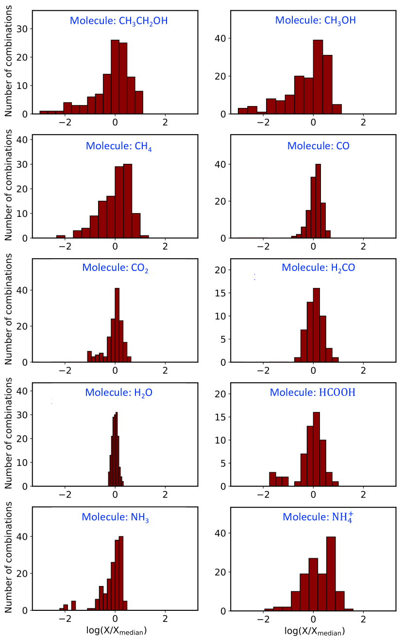
Figure 20: Log-transformed and median centered histograms of the ice column densities derived from all solutions inside 3$\sigma$ confidence interval in the case of Elias 29.