A comparison of cluster algorithms for the bond-diluted Ising model

Abstract

Monte Carlo cluster algorithms are popular for their efficiency in studying the Ising model near its critical temperature. We might expect that this efficiency extends to the bond-diluted Ising model. We show, however, that this is not always the case by comparing how the correlation times $\tau_{w}$ and $\tau_{\rm sw}$ of the Wolff and Swendsen-Wang cluster algorithms scale as a function of the system size $L$ when applied to the two-dimensional bond-diluted Ising model. We demonstrate that the Wolff algorithm suffers from a much longer correlation time than in the pure Ising model, caused by isolated (groups of) spins which are infrequently visited by the algorithm. With a simple argument we prove that these cause the correlation time $\tau_{w}$ to be bounded from below by $L^{z_{w}}$ with a dynamical exponent $z_{w}=\gamma/\nu\approx 1.75$ for a bond concentration $p<1$. Furthermore, we numerically show that this lower bound is actually taken for several values of $p$ in the range $0.5<p<1$. Moreover, we show that the Swendsen-Wang algorithm does not suffer from the same problem. Consequently, it has a much shorter correlation time, shorter than in the pure Ising model even. Numerically at $p=0.6$, we find that its dynamical exponent is $z_{\rm sw}=0.09(4)$.

I Introduction

The Ising model is one of the most popular models in statistical physics: its simplicity makes it easy to study while it is complex enough that many interesting physical phenomena can be studied with it, such as phase transitions and criticality [1]. Since its inception, numerous variants of the Ising model have been proposed to study different phenomena. An important class of such variants are the Ising models with impurities. These are used to investigate how the presence of impurities, which occur frequently in nature, affects the properties of a system. Common ways to model impurities in the Ising model is by randomly removing spins (site-dilution [2, 3, 4]), bonds (bond-dilution [5, 6, 7, 8, 9]) or alternatively by randomly modifying the strength of the interactions in some other way [6, 10]. In this paper we focus on the variant with bond-dilution.

The introduction of bond-dilution to the Ising model changes its properties significantly. For example, it has been shown that the critical temperature that separates the ferromagnetic and paramagnetic phases of the Ising model changes depending on the extent of the bond-dilution [8]. This even introduces a new type of phase transition because the critical temperature drops to zero at a certain bond concentration creating two phases (zero and non-zero critical temperature) separated by what is referred to as the percolation threshold [11]. In addition, it appears that the presence of impurities also alters the universality class of the model [2].

A common approach to study the Ising model is the use of Monte Carlo methods. The choice of the algorithm does not change any of the equilibrium properties: all algorithms sample the same (Boltzmann) distribution. However, the dynamics of different algorithms can vary strongly leading to pronounced differences in their efficiency for studying a certain model. In the pure Ising model, cluster algorithms such as the Wolff and Swendsen-Wang algorithms have proven themselves to be much more effective at criticality than single spin-flip algorithms like Metropolis [12]. This difference is expected to be even more pronounced in the bond-diluted Ising model since it has been recently shown that single spin-flip algorithms suffer from a diverging correlation time when the percolation threshold is approached [5]. The dynamics of cluster algorithms for the bond-diluted Ising model remains poorly studied and so it is still unclear whether they actually are more effective. Some studies have proposed that the efficiency of these cluster algorithms carries over to the bond-diluted Ising model and that correlation times actually decrease when site- or bond-dilution is introduced [13, 4]. We present a quantitative analysis of the dynamics of the Wolff and Swendsen-Wang algorithms to show that this is in fact not the case for the Wolff algorithm. We will demonstrate that the Wolff algorithm suffers from much longer correlation times than in the pure model, caused by isolated (groups of) spins, a fact which has previously been hinted at by Ballesteros et al, who showed that depending on the degree of bond dilution there are different regions, characterised by the size of the groups of isolated spins, where certain Monte Carlo updates are more efficient at thermalising the system [14]. We expand upon their work by proving a lower bound on the dynamical exponent of the Wolff algorithm and numerically showing that this lower bound is actually taken for several values of the dilution.

This paper is organised as follows. We first define the bond-diluted Ising model, the cluster algorithms, and the observables that we use. Next, we present our results and discuss what they teach us about the correlation times of the Wolff and Swendsen-Wang algorithms. In the final section we summarise our main findings and conclude.

II Model and Methods

II.1 Model

In this paper we study the bond-diluted Ising model in two dimensions on a square lattice of size $L\,\times\,L$. This model is a variant of the regular Ising model with nearest-neighbour interactions and is obtained by randomly removing a fraction $1-p$ of the bonds (i.e. interactions between two neighbours) from the lattice, where $p$ is called the bond concentration. Defined this way, $p$ is the probability that there is a bond between two neighbours. With this choice, $p=1$ corresponds to the regular Ising model and $p=0$ to a collection of isolated spins (no interactions). We define the model with the Hamiltonian

$$\mathcal{H}=-J\sum_{\langle ij\rangle}c_{ij}(p)s_{i}s_{j}$$ (1)

where the sum runs over all pairs of nearest-neighbour sites, $s_{i}=\pm 1$ is the spin on site $i$ and $c_{ij}(p)$ is a constant that follows a Bernoulli distribution with probability $p$, i.e. it has value $1$ with probability $p$ and value $0$ with probability $1-p$. We refer to a realization of the $c_{ij}$’s for all nearest-neighbour pairs as a configuration of the model. The bond-dilution is frozen in for a particular configuration. In other words, the values of the $c_{ij}$’s are fixed for a specific configuration. All through the manuscript, energy is measured in units of $J$.

II.2 Algorithms

We use the bond-diluted Ising model to study the behaviour, and in particular the dynamics, of two cluster Monte Carlo algorithms. The first of these is the Wolff algorithm [15]. The basic idea behind this algorithm is to grow a cluster of spins and flip all the spins in this cluster simultaneously with probability 1. To grow a cluster we perform the following steps [12],

1. choose a spin at random from the lattice,

2. consider each of its neighbours. If the spins are aligned, add the neighbour to the cluster with probability $1-e^{-2\beta J}$ with $\beta=\frac{1}{k_{B}T}$ and $J$ the coupling constant from the Hamiltonian,

3. for each of the neighbours added in step 2 also consider all their neighbours to be added to the cluster and repeat this until no more neighbours exist that have not yet been considered.

It can be shown that by growing the cluster in this way we satisfy both ergodicity and detailed balance [12]. It is important to note that in the bond-diluted Ising model two spins are only considered to be neighbours if there is a bond between them.

The second algorithm under consideration is the Swendsen-Wang algorithm [16]. Similar to the Wolff algorithm, clusters of spins are grown according to the aforementioned procedure. It differs, however, in the fact that we do not just grow a single cluster, but cover the entire lattice with clusters and flip each of these with probability $\frac{1}{2}$ in a single step [12]. Since clusters are grown in the same way as in the Wolff algorithm, showing that the Swendsen-Wang algorithm satisfies ergodicity and detailed balance proceeds analogously [12].

II.3 Observables

During our simulations we keep track of several quantities. This includes the energy of a state, which follows directly from the definition of the model and requires no further explanation. Additionally, we measure a quantity which we will refer to as the spin age and which we define as follows.

To extract more information about the dynamics of the Wolff algorithm from our simulations, we label each site in the lattice with a spin age $a_{i}$, which we define to be the time since site $i$ was last visited (i.e. was part of a Wolff cluster) measured in the number of Wolff cluster moves. In other words, when a site is visited, its age is set to $0$ and each subsequent Wolff cluster move where the site is not visited, the age is incremented by $1$. Once the system is thermalised, both with respect to its configuration of spins and the distribution of ages, we count how often a certain age occurs at various steps in the simulation, to produce a histogram showing the distribution of ages in equilibrium. To be specific, at certain steps in the simulation (between moves) we measure for each age $a$ how many spins in the lattice are labelled with that age at that step and we call this number the age frequency $f_{L}(a)$.

III Results and Discussion

III.1 The Wolff algorithm

We first discuss the behaviour of the Wolff algorithm applied to the bond-diluted Ising model. We will start with a simple argument to show that there must be a lower limit on the correlation time. Then we discuss the results from our numerical analysis to show that this lower bound is also taken for several values of the bond concentration $p$. But before going into the simple argument, let us first introduce some notation and two different time scales that we have used.

For all the results we measure time in cluster moves of the algorithm used, because we found this the most intuitive timescale for understanding the results. However, when evaluating the performance of an algorithm, we prefer to measure time such that it scales with required CPU time. Since the CPU time per single Wolff cluster move can vary significantly, we require a second timescale for the Wolff algorithm. A good candidate is to measure time such that $t=1$ corresponds to the situation where on average as many spins are flipped as there are in the lattice. The relation between the time $t$ and our previous time, which we denote by $t_{\mathrm{steps}}$ for Wolff, is given by $t=t_{\mathrm{steps}}\frac{\langle n\rangle}{L^{2}}$, where $\langle n\rangle$ is the average size of a Wolff cluster [12]. It can also be shown that $\langle n\rangle$ scales as $L^{\gamma/\nu}$ at the critical temperature such that $L^{\gamma/\nu-2}$ acts as a conversion factor when required [12]. By construction, the same number of spins, namely all the spins in the lattice, are visited by the Swendsen-Wang algorithm in each cluster move, so $t_{\mathrm{steps}}$ already scales with CPU time for Swendsen-Wang and there is no additional timescale meaning we use $t$ to denote the time measured in Swendsen-Wang cluster moves.

Now let us turn to the simple argument. We argue that the correlation time $\tau_{\mathrm{steps},w}$ for $p<1$ is bounded from below by $L^{2}$, i.e. $\tau_{\mathrm{steps},w}=\Omega(L^{2})$. To see this, note that for any $p<1$ there will always exist at least one isolated spin in the lattice for a sufficiently large system size (i.e. for a sufficiently large system the expectation value for the number of isolated spins will be at least 1). With an isolated spin we mean spins which have all their bonds to the rest of the lattice removed. Such spins would only be flipped by the Wolff algorithm if they are chosen as the seed spin. And since each spin is equally likely to be picked and there are $L^{2}$ spins, the correlation stored in these spins, however small it might be, will also survive for $\Omega(L^{2})$ cluster moves. Therefore, we can conclude that the correlation time $\tau_{\mathrm{steps},w}$ is bounded from below by $L^{2}$.

To study the behaviour numerically, we ran simulations with the Wolff algorithm for various system sizes with $p=0.6$ at $(\beta J)^{-1}=0.940$ where $\beta=\frac{1}{k_{B}T}$ and $J$ the coupling constant. We chose this value for $p$ because the effects of bond-dilution become more pronounced when the bond fraction $p$ is significantly below $1$. The temperature was chosen to be in the vicinity of the critical temperature as determined with the Binder cumulant. The value we found is also in good agreement with the critical temperature found in other papers, see for example [5]. Unless otherwise mentioned, we used $100,000$ different realizations of the bond dilution in each simulation.

Figure 1 shows the evolution of the energy of the system towards its thermal equilibrium value as a function of Wolff cluster moves. For $L=40$ we ran for 400 cluster moves per configuration, for $L=100$ we ran for 300 cluster moves and in between we tuned the number of cluster moves to roughly keep the CPU time used per simulation constant. At $t_{\mathrm{steps}}=0$, the system starts in the configuration with all spins pointing up ($s_{i}=1$ for all $i$). Notice how the curve seems to transition from a fast decay for small $t_{\mathrm{steps}}$ to a slower decay at large $t_{\mathrm{steps}}$. When the vertical and horizontal axes are scaled with $L^{2}$ the tails of the curves, the regions of slower decay, collapse. Since these tails are the limiting factor in convergence of the energy to its equilibrium this suggests that the correlation time $\tau_{\mathrm{steps},w}$ scales as $L^{2}$ such that $\tau_{w}$ scales as $L^{z_{w}}$ with $z_{w}={\gamma/\nu}$. Numerically, it is reported that $\gamma/\nu$ is independent of $p$ for $p\geq 0.6$, and actually indistinguishable from $\gamma/\nu=1.75$ as in the regular Ising model [8]. Note that, while the equilibrium exponents are numerically indistinguishable, the dynamic exponent is very different: in the regular two-dimensional (2D) Ising model the dynamic exponent is reported as $z_{w}=0.25(1)$ [12].

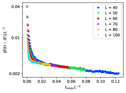
Figure 1: Convergence of the energy $E(t)$ to the thermal equilibrium $\langle E\rangle$ during thermalisation with the Wolff algorithm for different system sizes $L$ with $p=0.6$ at $(\beta J)^{-1}=0.940$ where $\beta=\frac{1}{k_{B}T}$ and $J$ the coupling constant. For $t_{\mathrm{steps}}=0$ the system starts in a state with all spins pointing up. Both the vertical and horizontal axes were scaled with $L^{2}$. Note the collapse of the right tails of the curves, suggesting that the correlation time $\tau_{\mathrm{steps},w}\sim L^{2}$.

To verify our argument that isolated (groups of) spins exist that are not touched by the algorithm for a long time, we computed a histogram of the distribution of the spin ages throughout a simulation with the Wolff algorithm in the manner described in the Model and Methods section. For these simulations we used $10^{4}$ realizations of the bond-dilution. To initialise the system we first thermalise with 50 Swendsen-Wang moves, starting from a state with all spins pointing up. We also first run the simulation for $5L^{2}$ Wolff cluster moves to make sure that spins can actually reach all the ages that we report in the histogram. Finally, we measure the age for an additional $1000$ consecutive Wolff steps. We did the simulations for both $p=0.6$ at $(\beta J)^{-1}=0.940$ as before as well as for $p=0.7$ at $(\beta J)^{-1}=1.310$, $p=0.8$ at $(\beta J)^{-1}=1.648$ and $p=0.9$ at $(\beta J)^{-1}=1.964$. For completeness, we also did the simulations at $p=1$ at $(\beta J)^{-1}=2.27$. We found these temperatures to be in the vicinity of the critical temperature at their respective bond fractions $p$, again in agreement with the critical temperature found in other papers [5]. The results are shown in figure 2.

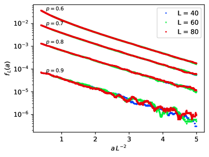
(a) $p<1$

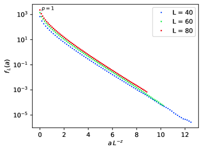
(b) $p=1$

Figure 2: Distribution of spin ages $a$ during a simulation with the Wolff algorithm at equilibrium. In figure (a) we see the data for $p=0.6$ at $(\beta J)^{-1}=0.940$, $p=0.7$ at $(\beta J)^{-1}=1.310$, $p=0.8$ at $(\beta J)^{-1}=1.648$ and $p=0.9$ at $(\beta J)^{-1}=1.964$. In figure (b) we see the data for $p=1$ at $(\beta J)^{-1}=2.27$. Here $\beta=\frac{1}{k_{B}T}$ and $J$ the coupling constant. The spin age is defined as the time since the site was last visited, measured in Wolff cluster moves. Note the different scaling of the horizontal axis for (a) and (b). The horizontal axis in (a) was scaled with $L^{2}$, while in (b) it was scaled with $L^{z_{\mathrm{steps},w}}$ where $z_{\mathrm{steps},w}=0.50$ was chosen to correspond with the $z_{w}=0.25(1)$ for the regular 2D Ising model [12]. The collapse of the curves in (a) again suggests that the correlation time $\tau_{\mathrm{steps},w}$ of the Wolff algorithm scales as $L^{2}$, in agreement with figure 1. Scaling the horizontal axis in (b) with the dynamical exponent for the regular 2D Ising model from the literature also leads to a reasonable collapse, as we would expect.

The figure clearly shows that some spins survive for a very long time. Also note the strikingly good collapse of the curves in 2a when we scale the horizontal axis with $L^{2}$, for $p=0.6$, $p=0.7$, $p=0.8$ and $p=0.9$. This supports our earlier finding that $\tau_{w}$ scales as $L^{z_{w}}$ with $z_{w}=\gamma/\nu\approx 1.75$ for these values of $p$. In contrast, the histogram drops to zero very quickly for $p=1$ and we need a different scaling to get a reasonable collapse. This seems to suggest that the effect of long surviving spins only shows up for $p<1$.

III.2 The Swendsen-Wang algorithm

We now turn our attention to the Swendsen-Wang algorithm. By construction, it visits every spin in the lattice each step, so it should not suffer from the problems encountered with the Wolff algorithm, originating from long surviving spins. Similar to the Wolff algorithm, we ran simulations for various system sizes $L$ at $p=0.6$ and $(\beta J)^{-1}=0.940$, i.e. the setup of the simulations was exactly the same, only the algorithm used to update the spins was different. Figure 3 shows the analogue of figure 1, but then for Swendsen-Wang. In addition, it contains an inset figure that shows the same data but plotted in a different way. At $L=30$ we ran for 300 Swendsen-Wang steps per configuration while at $L=100$ we ran for 100 steps; in between we tuned the steps to keep the CPU time used roughly constant. In the main part of the figure we can see that the energy quickly converges to its thermal equilibrium value and the slowly decaying tail from figure 1 is absent. Moreover, when scaling the vertical axis with $L^{2}$ and the horizontal axis with $L^{z_{\rm sw}}$ with $z_{\rm sw}=0.09(4)$, the curve collapse suggests that the correlation time $\tau_{\rm sw}$ for Swendsen-Wang at $p=0.6$ scales as $L^{z_{\rm sw}}$. The value for $z_{\rm sw}$ used to scale the horizontal axis was chosen to be the same as the value we determined with a different method which will be described below. Note that the dynamical exponent $z_{\rm sw}$ is significantly smaller at $p=0.6$ than for the regular 2D Ising model ($p=1$) where $z_{\rm sw}=0.25(1)$ [12]. This is the opposite of the super slowing down observed for the Metropolis algorithm [5]. Finally, in the inset figure the data for $h(t)$ versus time $t$ is plotted. Here $h(t)=-\log\left(c\left|E(t)-\langle E\rangle\right|\right)$ with $c=\left|E(0)-\langle E\rangle\right|^{-1}$. The blue curve is a straight line with slope $0.87$. Since the data seems to be parallel to this blue curve instead of a curve with slope $1$, the convergence of the energy seems to be a stretched exponential.

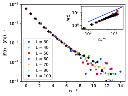
Figure 3: Convergence of the energy $E(t)$ to the thermal equilibrium $\langle E\rangle$ during thermalisation with the Swendsen-Wang algorithm for different system sizes $L$ with $p=0.6$ at $(\beta J)^{-1}=0.940$ where $\beta=\frac{1}{k_{B}T}$ and $J$ the coupling constant. For $t=0$ the system starts in a state with all spins pointing up. The vertical axis was scaled with $L^{2}$ and the horizontal axis with $L^{z_{\rm sw}}$ with $z_{\rm sw}=0.09(4)$, where $z_{\rm sw}$ was chosen to be the same as in figure 4. Note that this plot is equivalent to figure 1 but for the Swendsen-Wang algorithm. The collapse of the curves suggests that the correlation time for the Swendsen-Wang algorithm scales as $L^{z_{\rm sw}}$ with $z_{\rm sw}=0.09(4)$. Also note the absence of a slowly decaying tail, demonstrating that the Swendsen-Wang algorithm does not suffer from the same problems that plague the Wolff algorithm (see figure 1). The inset figure in the top-right shows the same data but plotted differently. Here $h(t)=-\log\left(c\left|E(t)-\langle E\rangle\right|\right)$ with $c=\left|E(0)-\langle E\rangle\right|^{-1}$. The blue curve is a straight line with slope $0.87$. Since the data seems to be parallel to this blue curve instead of a curve with slope 1, the convergence of the energy seems to be stretched exponential.

We have already shown that there is a value for the dynamical exponent $z_{\rm sw}$ that gives a good collapse of the data in figure 3. However, this plot shows data from simulations out-of-equilibrium so we did not use this data to determine the correct scaling of the correlation time (at least not in the form presented in figure 3). Instead, we determined it from equilibrium simulations. For this we computed the evolution of the mean-square displacement of the energy $\langle[E(t)-E(0)]^{2}\rangle$ from the same data as was used for figure 3. To obtain equilibrium data we discarded all data before the system was thermalised. For $L=30$ this concerns all data before $t=50$ and for all other system sizes all data before $t=20$ (i.e. these times became the new $t=0$ for determining $\langle[E(t)-E(0)]^{2}\rangle$). The results are shown in figure 4. After scaling the vertical axis with the numerically determined limiting values of the curves, we can collapse the curves using a horizontal scaling of $L^{z_{\rm sw}}$ with $z_{\rm sw}=0.09(4)$. The uncertainty in the dynamical exponent was determined by tuning the scaling of the axis to determine the range within which the collapse seemed good. The size of this range was then used as a measure of the uncertainty. This confirms our earlier numerical estimate of the dynamical critical exponent for the Swendsen-Wang algorithm at $p=0.6$.

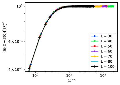
Figure 4: Mean-square displacement of the energy $\langle[E(t)-E(0)]^{2}\rangle$ in thermal equilibrium as a function of Swendsen-Wang moves $t$ for different system sizes $L$ with $p=0.6$ at $(\beta J)^{-1}=0.940$ where $\beta=\frac{1}{k_{B}T}$ and $J$ the coupling constant. The vertical axis was scaled with the numerically determined limit value of the curves, while the horizontal axis was scaled with $L^{z_{\rm sw}}$ with $z_{\rm sw}=0.09(4)$. The dynamical critical exponent for the Swendsen-Wang algorithm was determined by tuning the scaling of the horizontal axis until a good collapse was found.

IV Summary and Conclusions

We have shown how the correlation times $\tau_{w}$ and $\tau_{\rm sw}$ of the Wolff and Swendsen-Wang cluster algorithms scale as a function of the system size $L$ when applied to the 2D bond-diluted Ising model. We demonstrated that the Wolff algorithm suffers from a much longer correlation time than in the pure Ising model, caused by isolated (groups of) spins which are infrequently visited by the algorithm. With a simple argument we proved that these cause the correlation time to be bounded from below by $L^{z_{w}}$ where $z_{w}=\gamma/\nu\approx 1.75$ for a bond concentration $p<1$. Furthermore, we showed numerically that this lower bound is actually taken for several values of the bond concentration in the region $0.5<p<1$. Moreover, we have shown that the Swendsen-Wang algorithm does not suffer from the same problem, by construction. It has a much shorter correlation time, even shorter than in the pure Ising model. Numerically, we have found that its correlation time scales as $L^{z_{\rm sw}}$ with $z_{\rm sw}=0.09(4)$ at $p=0.6$.

We expect that the Wolff algorithm will suffer from the same problems in the three-dimensional bond-diluted Ising model, albeit to a lesser degree as more bonds will have to be removed to create isolated spins. In addition, we think the same will hold for the site-diluted and weakly diluted (i.e. where you weaken instead of removing the bonds) Ising models. This could be something to explore in the future.

References

- Brush [1967] S. G. Brush, History of the Lenz-Ising model, Reviews of modern physics 39, 883 (1967).
- Hasenbusch et al. [2007] M. Hasenbusch, F. P. Toldin, A. Pelissetto, and E. Vicari, The universality class of 3D site-diluted and bond-diluted Ising systems, Journal of Statistical Mechanics: Theory and Experiment 2007, P02016 (2007).
- Ballesteros et al. [1997] H. Ballesteros, L. Fernández, V. Martín-Mayor, A. M. Sudupe, G. Parisi, and J. Ruiz-Lorenzo, Ising exponents in the two-dimensional site-diluted Ising model, Journal of Physics A: Mathematical and General 30, 8379 (1997).
- Ivaneyko et al. [2005] D. Ivaneyko, J. Ilnytskyi, B. Berche, and Y. Holovatch, Criticality of the random-site Ising model: Metropolis, Swendsen-Wang and Wolff Monte Carlo algorithms, CONDENSED MATTER PHYSICS 8, 149 (2005).
- Zhong et al. [2020] W. Zhong, G. T. Barkema, and D. Panja, Super slowing down in the bond-diluted Ising model, Phys. Rev. E 102, 022132 (2020).
- Hasenbusch et al. [2008] M. Hasenbusch, F. P. Toldin, A. Pelissetto, and E. Vicari, Universal dependence on disorder of two-dimensional randomly diluted and random-bond Ising models, Phys. Rev. E 78, 011110 (2008).
- Zobin [1978] D. Zobin, Critical behavior of the bond-dilute two-dimensional Ising model, Phys. Rev. B 18, 2387 (1978).
- Hadjiagapiou [2011] I. A. Hadjiagapiou, Monte Carlo analysis of the critical properties of the two-dimensional randomly bond-diluted Ising model via Wang–Landau algorithm, Physica A: Statistical Mechanics and its Applications 390, 1279 (2011).
- Berche et al. [2004] P.-E. Berche, C. Chatelain, B. Berche, and W. Janke, Bond dilution in the 3D Ising model: a Monte Carlo study, The European Physical Journal B-Condensed Matter and Complex Systems 38, 463 (2004).
- Wolff and Zittartz [1983] W. Wolff and J. Zittartz, On the phase transition of the random bond Ising model, Zeitschrift für Physik B Condensed Matter 52, 117 (1983).
- Jain [1995] S. Jain, Anomalously slow relaxation in the diluted Ising model below the percolation threshold, Physica A: Statistical Mechanics and its Applications 218, 279 (1995).
- Newman and Barkema [1999] M. E. J. Newman and G. T. Barkema, Monte Carlo Methods in Statistical Physics (Oxford University Press, Oxford, 1999).
- Hennecke and Heyken [1993] M. Hennecke and U. Heyken, Critical dynamics of cluster algorithms in the dilute Ising model, Journal of statistical physics 72, 829 (1993).
- Ballesteros et al. [1998] H. G. Ballesteros, L. A. Fernández, V. Martín-Mayor, A. Muñoz Sudupe, G. Parisi, and J. J. Ruiz-Lorenzo, Critical exponents of the three-dimensional diluted Ising model, Phys. Rev. B 58, 2740 (1998).
- Wolff [1989] U. Wolff, Collective Monte Carlo updating for spin systems, Phys. Rev. Lett. 62, 361 (1989).
- Swendsen and Wang [1987] R. H. Swendsen and J.-S. Wang, Nonuniversal critical dynamics in Monte Carlo simulations, Phys. Rev. Lett. 58, 86 (1987).