Non-local Potts model on random lattice and chromatic number of a plane

Abstract

Statistical models are widely used for investigation of complex system’s behaviour. Most of the models considered in the literature are formulated on regular lattices with nearest neighbour interactions. The models with non-local interaction kernels have been less studied. In this article we investigate an example of such a model – non-local $q$-color Potts model on a random $d=2$ lattice. Only the same color spins at unit distance (within some small margin $\delta$) interact. We study the vacuum states of this model and present the results of numerical simulations and discuss qualitative features of the corresponding patterns. Conjectured relation with the chromatic number of a plane problem is discussed.

• August 2021

Keywords: Potts model, Non-local interaction, Hadwiger-Nelson problem

1 Introduction

Statistical models on discrete lattices are proved to be an extremely useful tool in studying various problems in fundamental and applied science. The best known is certainly the Ising model and its generalizations like the Potts models family [1, 2]. As is well known, the typical model of this kind is defined by the functional

$$H=\sum_{i,k\in M}\>J_{ik}\>\sigma_{i}\cdot\sigma_{k},$$ (1)

where the dynamical variables $\sigma_{i}$ - ”spins” - take values in some set $S$, while the indices $i$, $k$, run over the lattice $M$. The matrix $J_{ik}$ encodes the ”interaction strength” between sites $i$ and $k$. It is usually assumed that $S,M,J_{ik}$ and the composition law are such that $H$ is a real non-negative number for any spin configuration. The two most common problems are finding the vacuum state of (1), i.e. the configuration(s) $\{\sigma_{i}\}$, which provide(s) minimum of $H$, and computation of the corresponding partition function

$$Z=\sum_{\{\sigma_{i}\}}\>e^{-\beta H}.$$ (2)

In the low temperature limit the latter one is dominated by the vacuum state(s) contribution, but needless to say that computing (2) and studying its $\beta\to\infty$ limit is usually by far not the most economic way to find the vacuum state(s) of a model.

The most peculiar feature of all these models is a subtle interplay between a structure of the space $S$ the degrees of freedom belong to, and geometry and topology of the bulk, encoded in $M$ and the interaction kernel $J_{ik}$. In particular, if the model in question undergoes phase transition at some value of the inverse temperature $\beta$, the typical correlation length in the vicinity of this point can be much larger than the scale of the microscopic structure of the lattice. As a result, large distance correlators become insensitive to this structure and can correspond to some continuous theory in this limit, which shares with the original model only some global parameters like dimension or topology. However if one is far from the phase transition point, the lattice microstructure is manifest. For example, in the ground state of the standard nearest neighbor antiferromagnetic Ising model the typical correlation length equals to just one lattice link and the concrete pattern of the spins in this lowest state depends on the geometry of the lattice (hypercubic, honeycomb etc).

There is another well known way to get rid of the dependence on the lattice microstructure - to define the model on a random lattice. This is the framework we work within in the present paper. The clear disadvantage of this method is an absence of a fixed geometry. Therefore the only geometric invariant can be given by the coupling pattern. We consider two-dimensional case with the interaction kernel, describing interaction of the given spin with all spins, whose distance from it is larger than $R-\delta/2$ but smaller that $R+\delta/2$:

$$J_{ik}=\left\{\begin{array}[]{ll}J,&\;\;R-\frac{\delta}{2}\leq|i-k|\leq R+\frac{\delta}{2}\\ 0,&\;\;\mbox{otherwise.}\end{array}\right.$$ (5)

We will assume that $\delta\ll R$, so the interaction region can be thought of as a ring.

For a regular lattice the above means that the number of neighbors is the same for any spin. For example, in the $d$-dimensional Ising model on a hypercubic lattice with the link $R$ it is exactly $2d$ for any $0<\delta\ll R$.

For a random lattice, let us take $N$ sites to be randomly distributed over a compact $d$-dimensional region with linear size $L$, so we get $\rho=N/L^{d}$ for the average site density. Then the average number of each spin neighbors is given by $\rho\sim R^{d-1}\delta$. It is easy to see that if one requires that each spin to have at least one neighbor on average, there will be $\sim R^{d}\rho\gg 1$ noninteracting spins, which are closer to the chosen one, than the neighbors it interacts with. This is a peculiar difference between statistical models on regular and random lattices: interaction at the fixed (minimal) distance (within perhaps some margin $\delta$) is the same thing as interaction with the nearest neighbors for the former, but not for the latter ones.

We proceed below with the analysis of (1) on a plane ($d=2$) with the interaction kernel (5). The spins $\sigma_{i}$ are represented by $q$-component vectors (we use the word ”colors” for different components of these vectors), $\sigma_{i}=(\sigma_{i}^{1},\sigma_{i}^{2},...,\sigma_{i}^{q})$ where $\sigma_{i}^{k}\in\{0,1\}$ and $\sum_{k=1}^{q}\sigma_{i}^{k}=1$, so the product $\sigma_{i}\cdot\sigma_{k}=1$ if spins in the sites $i$ and $k$ have the same color, and $\sigma_{i}\cdot\sigma_{k}=0$ otherwise.

The idea of nearest neighbor interaction goes to physical interpretation of the degrees of freedom as spins whose interaction decreases with the distance and hence is the strongest between the closest spins. The non-local interaction models have attracted much less attention in the literature (see however [3, 4, 5, 6, 7]). In the present paper we consider the model with interaction at finite distance, i.e. the spins interact when they are located within some finite distance from each other. This model can be seen as a discrete version of the combinatorial topology problem of unit graph coloring. This problem is known in mathematical literature under the name Hadwiger-Nelson problem (hereafter referred to as EHN problem, E stands for Paul Erdos who made significant contribution to this topic [8, 9]) and can be formulated as follows: what is the minimal number of colors $q$ one has to use to color the $\mathbf{R}^{d}$ space in such a way that no two points at unit distance are colored identically [10]. There is a vast mathematical literature on the subject [8, 9, 11, 12]. Let us summarize the main findings here. In the $d=1$ case the EHN problem has a trivial solution $q=2$ and the minimal configuration is shown in the figure 1. Surprisingly, already for a plane ($q=2$) an answer is unknown. It can be easily shown that $q=3$ colors is not enough (figure 2a), while for $q=7$ a regular partition satisfying the requirement exists (figure 2b). Of course, the solution shown in the figure 2b is not unique. Quite recently it was argued with the help of a sophisticated mathematical construction that $q=4$ is also too small [13]. So, one is left with three possibilities: $q=5$, $q=6$ or $q=7$.

Figure 1: The solution of EHN problem for one dimension – the alternating lines of unit length with one excluded point (at the right edge in our example).

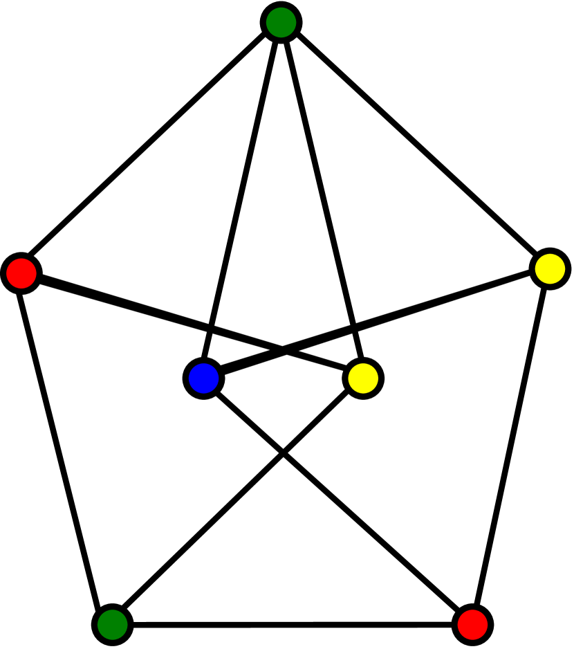
(a)

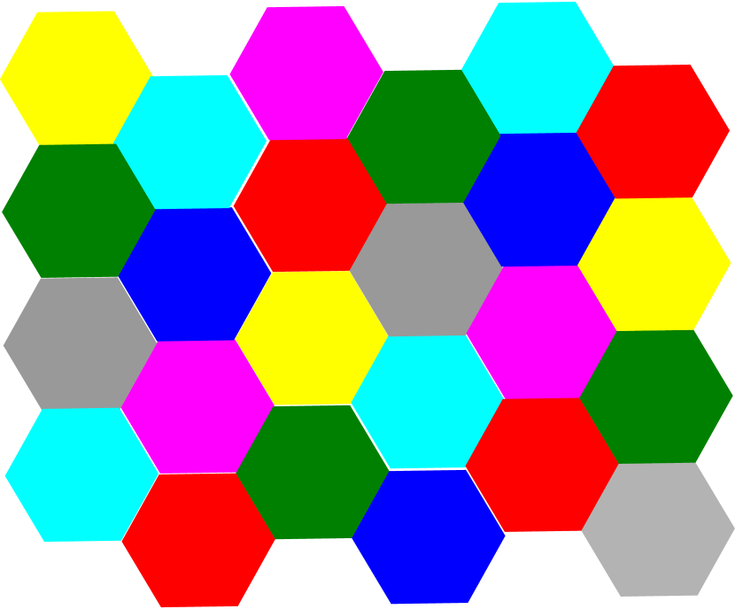
(b)

Figure 2: Illustration of the fact that $4\leqslant q\leqslant 7$: (a) The Moser’s spindle – four-chromatic unit distance graph on 11 vertices proving the necessity of minimum 4 colors for coloring plane such that there are no points of the same color at the unit distance apart; (b) The coloring of the plane with 7 colors such that there are no points of the same color at the unit distance apart.

The intrinsic mathematical difficulty of the EHN problem has its roots in the necessity to assign discrete index of color $k=1,..,q$ to each point of the continuum set $\mathbf{R}^{d}$. The minimal configuration for $q=7$ is characterized by clustering of the plane in finite size domains, which renders the problem from continuum to countable set. It could happen that other kinds of solutions do exist (for the same value $q=7$ or for smaller $q$), where the points on the line connecting any two points (however close) have colors, different from the colors of the edge points. Such ”fractal colorings” have no intrinsic ultraviolet scale.

In the settings (1), (5) a limit corresponding to the original EHN problem would be recovered as $N\to\infty$, $L\to\infty$, $\delta\to 0$, while $R=1$ without loss of generality. The EHN problem in this language is to find (for a given $q$) a configuration corresponding to $H=0$.

2 The method

2.1 Setting up the problem

First, let’s make some refinements in equation (1) describing energy function $H$ of the system. It can be normalized by introducing the normalization factor $A$:

$$E=A\sum\limits_{x,y}J_{xy}\delta_{i(x)i(y)}$$ (6)

and we assume $A=1$ in what follows. The alternative choice $A=\frac{L^{2}q}{2\pi R\delta N^{2}}$ would correspond to the energy of random configuration of the order of unity. In the expression (6) interaction kernel is given by (5), $i(x)$ – the color of the site $x$, $\delta_{i(x)i(y)}$ – Kronecker delta. The schematic picture is shown in the figure 3. The important parameter of this model is the averaged number of interacted neighbors for each particle. It is given by relation

$$\langle n\rangle=2\pi\delta\frac{N}{L^{2}}.$$ (7)

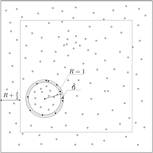
(a)

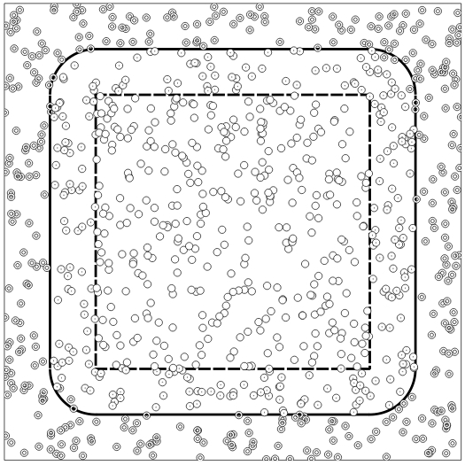
(b)

Figure 3: (a): The schematic picture of the model. A particle at the center of the ring interacts only with its ring-neighbors, which are, by definition, particles at $R\pm\delta/2$ distance from the chosen one. The dotted square represents area outside of which the colors of particles are fixed - the implementation of fixed boundary conditions; (b): The schematic picture of energy zones. All particles have the same properties but depicted differently depending on the zone they belong to. The inside energy is calculated only between open circled particles and each pair of them counted twice. Pairs which constitute of one open circled particle from inside zone and dotted circled particle from adjoining zone counted once. They contribute to outside energy. The interaction of pairs of dotted circled particles doesn’t contribute to energy. Interactions with ring symbol particles also omitted. It is worth mentioning that one should not be deluted by sparse density of particles - in reality the density is much higher and the example is given only for illustrative purposes.

In our work we fix this number as $\langle n\rangle=50$. This number is large enough to observe the basic properties of the model but at the same time allows to perform computations in reasonable time. Also we fix the linear size of area $L=20$ and width of interaction ring $\delta=0.02$. This corresponds to the number of sites equal to $N=159\,155$. All our simulations are based on this setup.

The true minimum $E=0$ is reached only if there are no particles of the same color that are ring-neighbours and, as should be clear from the above discussion, there is no way to get $E=0$ for small values of $q$. There are two questions in this respect: first, what are the typical patterns for minimized $E$ (for small as well as for large $q$) and, second, for which $q$ the energy $E$ approaches zero (perhaps, within statistical errors).

Another important thing is the boundary conditions. The most common are periodic conditions. However in our case it is not suitable because of non-local nature of the model. The non-locality $R$ leads to artificial effects depending on whether $L/R$ is integer or not, where $L$ is linear size of the domain. Therefore fixed boundary conditions, illustrated in the figure 3a, are more convenient. Particles outside dotted area stay unchanged through the process of minimization. Due to the fact that this belt of particles with fixed color makes an influence on particles inside, the energy of the system should be calculated at some distance from the border. We have chosen to compute energy in internal region with the size 11 $\times$ 11 (dotted line in the figure 3b). The energy $E$ is the sum of two components: the energy $E_{\mathrm{ins}}$ of interaction only between particles that are inside energy area and the energy $E_{\mathrm{out}}$ of interaction of particles located inside area with particles outside. The schematic picture is represented in the figure 3b. The total energy $E$ is given by

$$E=2E_{\mathrm{ins}}+E_{\mathrm{out}}.$$ (8)

It should be pointed out that energies $E_{\mathrm{ins}}$ and $E_{\mathrm{out}}$ are both non-negative quantities. Therefore vanishing of total energy in the given region implies vanishing of energy in any internal area of it.

2.2 The algorithm

The simplest possible algorithm is the greedy one, which accepts new configuration only if its energy smaller or equal. The well known drawback of this procedure is the tendency of the system to fall into the closest state, corresponding to the local minimum, which can be quite far from the global minimum. The simulated annealing algorithm [14] suits much better for this task and differ from greedy algorithm by possibility of accepting state with higher energy. The probability of such event decreases over the time and eventually system comes to the state which we consider as vacuum state. The algorithm starts from initial configuration of randomly distributed and colored particles and goes throw all of them in random order. The positions of particles are fixed while their colors are changed to random color at every step. If the energy decreases or stays unchanged then new color is accepted. But if the energy increases then new color is accepted with probability $P=\exp[(E-E^{\prime})/T]$, where $E$ is the energy of current state, $E^{\prime}$ is the energy of new state and $T$ is artificial temperature which decreases as some function of the step number. By trying different decrease functions we have chosen linear dependence, corresponding to $T_{n+1}=T_{n}-\Delta T$. After visiting all particles the $T$ is decreased and above process is repeated until the temperature reaches zero. As algorithm is running the probability of accepting configuration with higher energy is going down making harder for the system to leap between minima.

3 Results

Table 1: The parameters of simulated model

Quantity	Description	Value
$R$	radius of interaction	1.0
$\delta$	width of interaction	0.02
$L$	linear size of area	20.0
$N$	the number of particles	$159\,155$
$q$	the number of colors	2..7
$l_{\mathrm{f}}$	the width of fixed boundary	1.01
$L/(R\sqrt{N})$	ratio of average distance between points to $R$	0.05
$2\pi RN\delta/L^{2}$	average number of neighbors the spin interacts with	50

Relevant parameters of our model are summarised in the table 1. For each choice of $q$ we made 200 runs from random configurations and every run generated new random coloring of particles keeping positions the same. We also checked the case when positions were generated randomly for each run but did not find any difference. Below we present the results for different number of colors.

3.1 $q\leqslant 4$

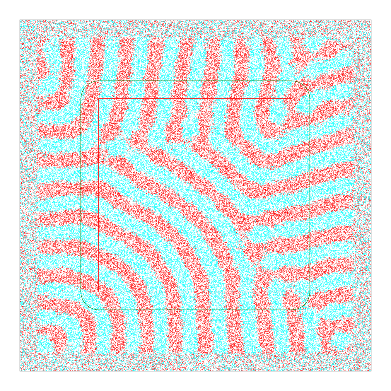
(a)

(b)

Figure 4: Typical vacuum configurations. (a): $q$ = 2; (b): $q$ = 3

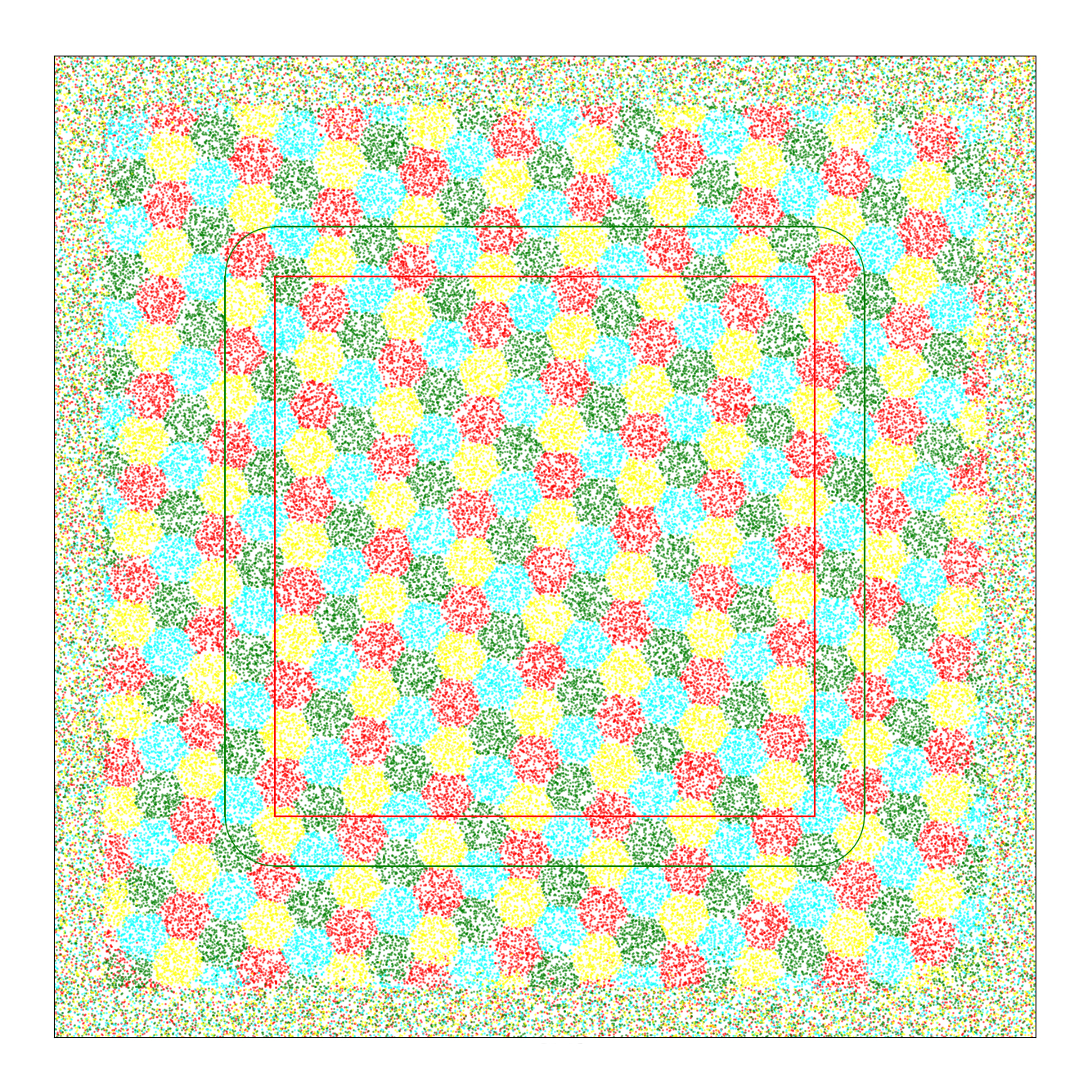
(a)

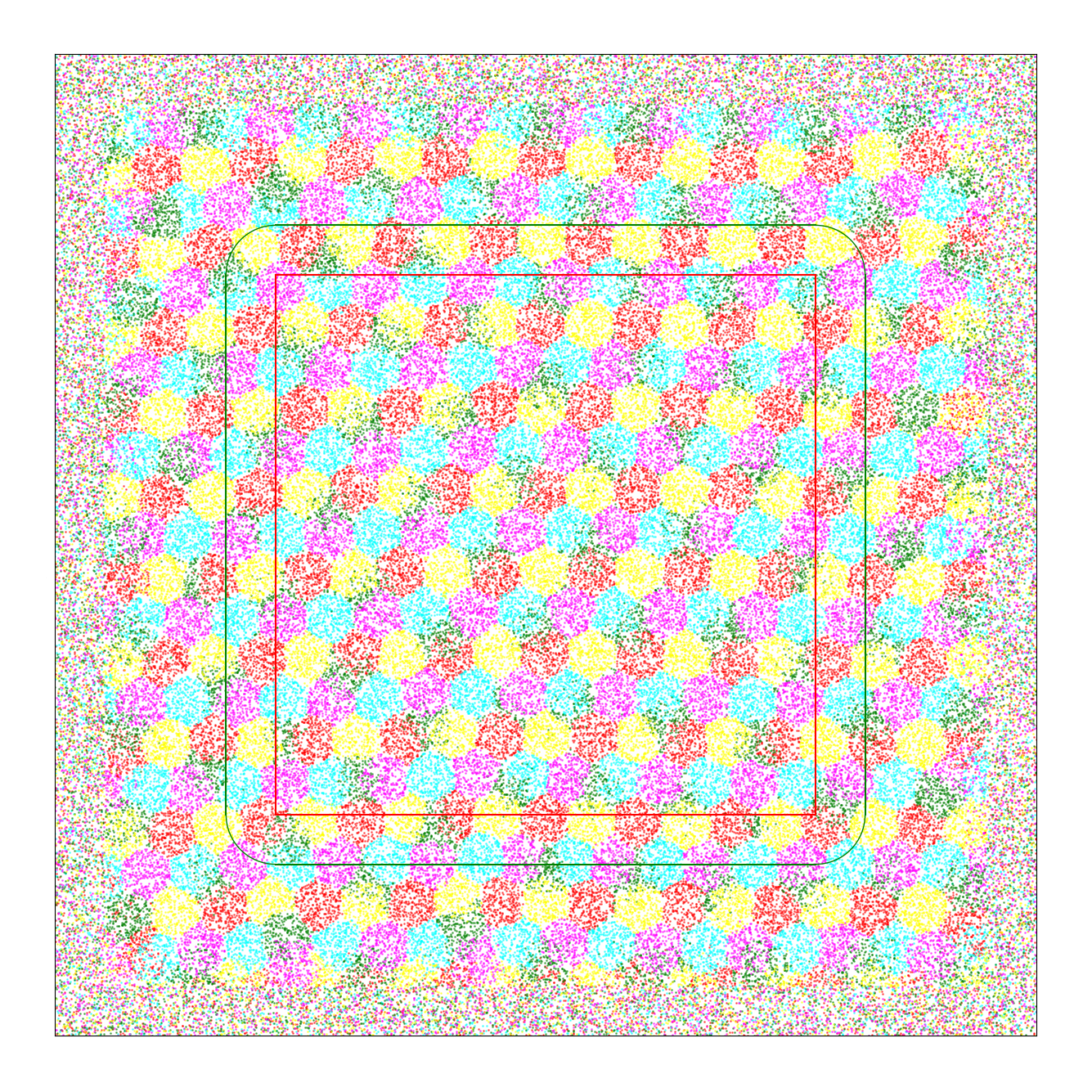
(b)

Figure 5: Typical vacuum configurations. (a): $q$ = 4; (b): $q$ = 5

Let us begin with $q=2$ colors. Typical minimized configuration are represented by alternate stripes pattern and shown in the figure 4a. The energy of such configuration is about 65% of the initial configuration energy, corresponding to random coloring.

For $q=3$ the resulting pattern is hexagonal and consist of regular shapes (figure 4b). The minimal energy is about 31% of the starting configuration. This number refers to regular almost pure pattern which emerges in 70% of minimizations. It is interesting that the resulting tiling is not ideal hexagonal lattice. If one constructs such lattice with optimal length of hexagon’s edge $l=0.64$ then the energy of it would be higher than energy of minimized configuration, with the ratio of energies of minimized configuration and regular lattice configuration is about 0.86. Some nontrivial mixing at the borders of the color clusters leads to decreasing of energy comparing to ideal regular hexagonal configuration.

For the case of $q=4$ the vacuum energy is about 3% of the initial configuration energy, but this energy is still far from zero value. The minimized configuration have regular hexagonal pattern as for $q=3$ (figure 5a). The nearly perfect coloring observed in 40% of configurations, the other part have some irregularities. The truly perfect coloring, as well as for $q=3$ does not give a minimum of energy. Considering optimal $l=0.56$ we get ratio about 0.7 that even less than corresponding ratio for three colors. It is remarkable how unnoticeable to naked eye changes on the edges of hexagons make such a big effect. Summarizing results for small $q$’s in the context of EHN problem we would not expect to see zero energy for $q\leqslant 4$. In the next section we discuss $q\geqslant 5$ case.

3.2 $q\geqslant 5$

We will go in reversed order and start with $q=7$ for the reason that it is an upper boundary of solution to EHN problem and therefore for discrete version of this we should get zero energy of vacuum configurations. It is a good test of our model and minimization algorithm. The tiling in the figure 2b allows pretty wide range of changing the length $l$ of the hexagon’s edge, $E=0$ for $l\in(\frac{1}{\sqrt{7}},\frac{1}{2})$. To put on test the simulated annealing algorithm we minimized initial configuration with randomly colored particles and observed zero vacuum energy on 97.5% of configurations. The example shown in the figure 6a. When we increased the number of neighbors $\langle n\rangle$ by the factor 2 (correspondingly increasing $N$), we got zero energy for standard offset on 41% configurations. We have found no vacuum configuration with the ideal hexagonal tiling but nevertheless the regular hexagonal pattern is observed. The result is a juxtaposition of regular lattices of clusters for each color.

For $q=6$ the minimized pattern is the same. Configurations with zero vacuum energy arise in about 4% of cases. The vast amount of minimizations end up at the vicinity of zero. The comparison histogram for six and seven colors is shown in the figure 7a. The example of configuration with zero energy is given in the figure 6b. It is obviously that if one would construct regular hexagonal tiling drawing analogy with $q=7$ (figure 2b) then the energy of resulting configuration would be not zero. What is surprising is how far actually it is from energy of minimized configurations. The energy of optimal hexagonal configuration with the edge of hexagon $l=0.55$ is $E=15\,740$ in contrast to around zero values for resulting vacuum configurations.

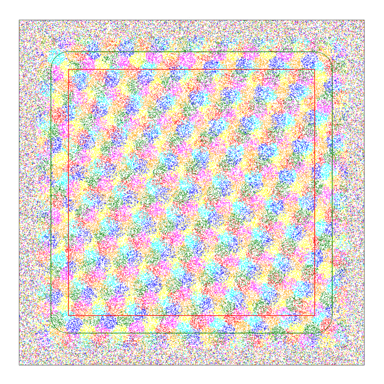
(a)

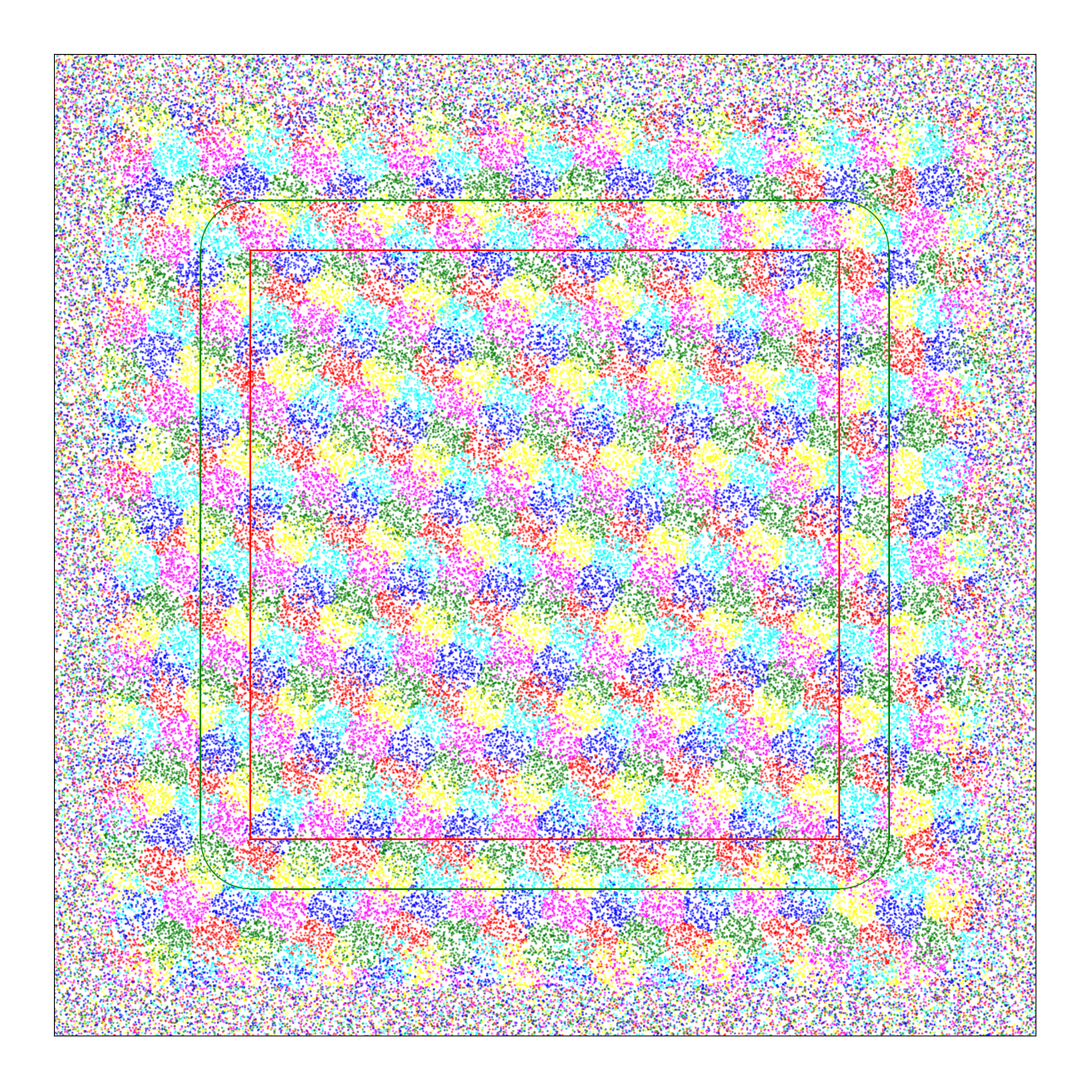
(b)

Figure 6: Examples of vacuum configurations with $E=0$. (a): $q$ = 7; (b): $q$ = 6.

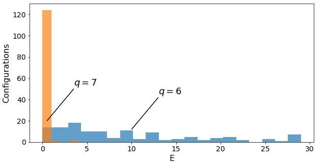
(a)

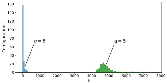
(b)

Figure 7: Comparison of distributions of energies for (a): six and seven colors, 127 the lowest energy configurations; (b): five and six colors, 200 configurations.

Finally we move to the description of minimized configurations for $q=5$. The typical pattern is shown in the figure 5b. Like for $q=4$ it also has hexagonal tiling but in this case only four colors form the pattern. The fifth color is displaced. Corresponding clusters of particles have pretty random shape and number of particles as well as the role of displaced color could go from one color to another in different parts of the area. Thus we observe the interesting conflict between color and geometric symmetries, and the former got broken as a result of this conflict. The energy of minimized configuration comprises only about 1% of energy of starting configurations. Nevertheless there is a huge gap between distributions of the energies for five and six colors (figure 7b). So based in our numerical results we can conjecture that there is no zero energy vacuum for five colors. We will discuss this issue below.

3.3 Breaking of color symmetry

The observed color symmetry breaking for $q=5$ is a consequence of the well known fact that no fifth order crystallographic symmetry does exist. To get quantative representation of this effect we check the ratio of particles with least represented color $N_{\mathrm{minc}}(A)$ to whole number of particles $N(A)$ inside particular region. The ratio scaled by $q$ depends on the area, as seen in the figure 8a. The curves for initial random coloring and minimized configurations are quite different. What is interesting that even for relatively big areas the second curve doesn’t approaches the first. So the effect is very profound and have rather global than local significance. For comparison one can look at the same graph for $q=3$ (figure 8b). In this case these curves go along together. The general picture is shown in the figure 9. From this we see that color symmetry breaking is not something that intrinsic only to $q=5$. Surprisingly it also shows up for six and seven colors (even for $q=4$) but in far less extent.

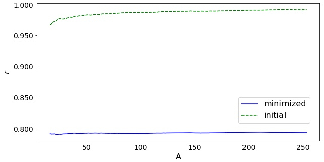
(a)

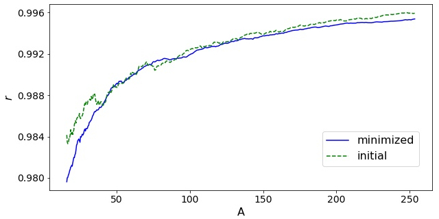
(b)

Figure 8: The ratio of number of particles with least represented colors to the total number of particles. (a): five colors; (b): three colors.

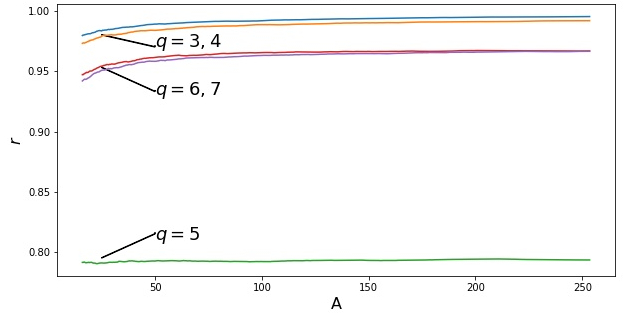
Figure 9: The ratio of number of particles with least represented colors to the total number of particles for all colors. The three levels are observed. The top two curves correspond to three and four colors, the intermediate ones to six and seven colors whereas bottom curve represents five colors.

4 Discussion

We discussed non-local Potts model in this paper. While in the local model the nearest neighbour interaction could imply anti-ferromagnetic state, when the interaction takes place at some finite distance, the picture is much more complex. We have found peculiar patterns in the ground states, strongly dependent on the number of ”colors” $q$ - degrees of freedom of the Potts spins. There are two most remarkable observations. First, we found color symmetry breaking for $q=5$ corresponding to the absence of degree five symmetry group of the plane. The geometric symmetry outperforms the color symmetry - the system minimizes its energy by quasi-regular pattern with nonequal share of one color with respect to four other ones. Of course, each color can be least represented, the actual choice depends on an initial configuration. Another observation comes from relation of our model to well known ENH problem of graph coloring in combinatorial topology. It was shown analytically [13] earlier that four colors are not enough for proper coloring of the plane and our numerical results agree with this conclusion. Moreover, we have found not a single zero energy configuration for $q=5$. On the other hand, zero energy vacuum state known for $q=7$, is clearly seen by our simulations. The situation with $q=6$ needs further refinements and, in ideal case, more systematic work towards the continuum limit (which is $N\to\infty$, $\delta\to 0$ our case). We hope to continue this analysis in future.

References

References

- [1] Beaudin L 2007 Rose-Hulman Undergraduate Mathematics Journal 8(1)
- [2] Wu F 1982 Rev. Mod. Phys. 54(1) 235–268
- [3] Werlberger M, Unger M, Pock T and Bischof H 2012 Efficient minimization of the non-local potts model SSVM ed Bruckstein A M, ter Haar Romeny B M, Bronstein A M and Bronstein M M (Springer Berlin Heidelberg) pp 314–325
- [4] Anderson A, Chaplain M and Rejniak K 2007 Single cell-based models in biology and medicine (Birkhauser)
- [5] Hou Z, Zong Y, Sun Z, Ye F, Mason T and Zhao K 2020 Nature communications 11(2064)
- [6] Schilling T, Pronk S, Mulder B and Frenkel D 2005 Physical Review E 71(036138)
- [7] Bauert T, Merz L, Bandera D, Parschau M, J S and Ernst K 2009 J. Am. Chem. Soc. 131 3460–3461
- [8] Erdos P 1961 Publ.Math.Inst Hung. Acad. Sci 221–254
- [9] Erdos P, Harary F and Tutte W T 1965 Mathematica 118–122
- [10] Hadwiger H 1961 Elemente der Math. 103–104
- [11] Guldan F 1991 Mathematica Bohemica 116 309–318
- [12] Moser L and Moser W 1961 Canad. Math. Bull. 4 187–189
- [13] de Grey A D 2018 The chromatic number of the plane is at least 5 arxiv:1804.02385
- [14] Kirkpatrick S, Gelatt C D and Vecchi M P 1983 Science 220 671–680