The Local Hole: a galaxy under-density covering 90% of sky to $\approx 200$ Mpc

Abstract

We investigate the ‘Local Hole’, an anomalous under-density in the local galaxy environment, by extending our previous galaxy $K-$band number-redshift and number-magnitude counts to $\approx 90$% of the sky. Our redshift samples are taken from the 2MASS Redshift Survey (2MRS) and the 2M++ catalogues, limited to $K<11.5$. We find that both surveys are in good agreement, showing an $\approx 21-22\%$ under-density at $z<0.075$ when compared to our homogeneous counts model that assumes the same luminosity function and other parameters as in our earlier papers. Using the Two Micron All Sky Survey (2MASS) for $n(K)$ galaxy counts, we measure an under-density relative to this model of $20\pm 2\%$ at $K<11.5$, which is consistent in both form and scale with the observed $n(z)$ under-density. To examine further the accuracy of the counts model, we compare its prediction for the fainter $n(K)$ counts of the Galaxy and Mass Assembly (GAMA) survey. We further compare these data with a model assuming the parameters of a previous study where little evidence for the Local Hole was found. At $13<K<16$ we find a significantly better fit for our galaxy counts model, arguing for our higher luminosity function normalisation. Although our implied under-density of $\approx 20\%$ means local measurements of the Hubble Constant have been over-estimated by $\approx 3$%, such a scale of under-density is in tension with a global $\Lambda$CDM cosmology at an $\approx 3\sigma$ level.

1 Introduction

Distance scale measurements of the expansion rate of the Universe or Hubble’s Constant, $H_{0}$, have improved significantly over recent years. For example, estimates of $H_{0}$ calculated by Riess et al. (2016) find a best fit value of $H_{0}=73.24\pm 1.74$ km s^-1 Mpc^-1, a quoted accuracy of 2.4%. However, this result is in serious tension with $H_{0}$ predictions made through $\Lambda$CDM model fits to the Planck CMB Power Spectrum. This ‘early Universe’ measurement yields a value of $H_{0}=67.4\pm 0.5$ km s^-1 Mpc^-1 (Planck Collaboration et al., 2018), which presents a tension at the $3-4\sigma$ level with measurements made using the local distance scale (see also Riess et al., 2018b).

These authors recognise the possibility that a source of the $\sim 9\%$ discrepancy between the $H_{0}$ measurements is unaccounted systematic uncertainties in one of, or both of the distance scale and early Universe approaches. However, an alternative proposal lies in studies of the galaxy distribution in the local Universe by Shanks (1990), Metcalfe et al. (1991), Metcalfe et al. (2001), Frith et al. (2003) & Busswell et al. (2004), who find evidence for an under-density or ‘Local Hole’ stretching to $150-200\,h^{-1}$ Mpc in the local galaxy environment.

Notably, Whitbourn & Shanks (2014) (hereafter WS14) suggest that the tension in $H_{0}$ measurements may arise from the outflow effects of the Local Hole. They find a detected under-density of $\approx 15\pm 3\%$ in number-magnitude counts $n(m)$ and redshift distributions $n(z)$, measured relative to a homogeneous model over a $\sim 9,000$ square degree area covering the NGC and SGC. This under-density is most prominent at $K<12.5$ and leads to an $\sim 2-3\%$ increase in $H_{0}$ which alleviates the tension to a $5\%$ level. Further, Shanks et al. (2019a) suggested that Gaia DR2 parallaxes might not have finally confirmed the Galactic Cepheid distance scale as claimed by Riess et al. (2018b) and could at least superficially, help reduce the overall tension to $<1\sigma$.

Moreover, the existence of the Local Hole has been detected in wider cluster distributions, with Böhringer et al. (2015), Collins et al. (2016) and Böhringer et al. (2020) finding underdensities of $\sim 30\%$ in the X-Ray cluster redshift distributions of the REFLEX II and CLASSIX surveys respectively. These results are in strong agreement with the galaxy counts of WS14, and suggest that the observed $H_{0}$ within the under-density would be inflated by $5.5^{+2.1}_{-2.8}\%$.

Contrastingly, Riess et al. (2018a) critique the assumption of isotropy and spherical symmetry assumed in the modelling of the Local Hole, highlighting that the WS14 dataset covers only $20\%$ of the sky, yet measurements drawn from this subset are projected globally to draw conclusions on the entire local environment. These authors further suggest that such an all-sky local under-density would then be incompatible with the expected cosmic variance of mass density fluctuations in the $\Lambda$CDM model at the $\approx 6\sigma$ level. In addition, Kenworthy et al. (2019) failed to find dynamical evidence in the form of infall velocities for the Local Hole in their Pantheon supernova catalogue.

Further, through analyses of the galaxy distribution in the 2M++ Catalogue, Jasche & Lavaux (2019), following Lavaux & Hudson (2011) (hereafter LH11) find that local structure can be accommodated within a standard concordance model, with no support for an under-density on the scale suggested by WS14. However, Shanks et al. (2019b) (see also Whitbourn & Shanks 2016) question the choice of the Luminosity Function (LF) parameters used by Jasche & Lavaux (2019) and LH11.

In this work we will examine two aspects of the above arguments against the Local Hole. First, to address the premise that the conclusions of WS14 cover too small a sky area to support a roughly isotropic under-density around our position, we will extend the analysis of WS14 and measure $K-$ band $n(m)$ and $n(z)$ galaxy counts over $\approx 90$% of the sky to a limiting Galactic latitude $|b|\ga 5^{\circ}$.

Second, we will compare the $n(z)$ and $n(K)$ model predictions of WS14 with Lavaux & Hudson (2011), hereafter LH11. These predictions will be compared at both the bright 2MASS limit and at the fainter $K-$band limit of the GAMA survey to try and understand the reasons for the different conclusions of WS14 and LH11 on the existence of the ‘Local Hole’.

2 Data

2.1 Photometric Surveys

We now detail properties of the photometric surveys used to provide $n(m)$ counts, alongside calibration techniques and star-galaxy separation methods that we apply to ensure consistency between the photometric data and model fit. Following WS14, we choose to work in the Vega system throughout. Thus for the GAMA survey, we apply a $K-$band conversion from the $AB$ system according to the relation determined by Driver et al. (2016):

$$K_{s}(Vega)=K_{s}(AB)-1.839$$ (1)

2.1.1 2MASS

The Two Micron All Sky Survey, 2MASS (Skrutskie et al., 2006) is a near-infrared photometric survey achieving a 99.998% coverage of the celestial sphere. In this work we will take $K$-band $n(m)$ counts from the 2MASS Extended Souce Catalogue (2MASS$\_$xsc), which is found to be $\sim 97.5\%$ complete (McIntosh et al., 2006), with galaxies thought to account for $\approx 97\%$ of sources.

For the galaxy $n(m)$ results, we choose to work in Galactic coordinates, and present counts from down to a limiting Galactic latitude $|b|>5^{\circ}$ except for the Galactic longitude range, $330<l<30^{\circ}$ where our limit will be $|b|>10^{\circ}$. This is the same 37063 deg² area of sky used by LH11. These cuts are motivated by the increasing density of Galactic stars at lower latitudes and close to the Galactic Centre.

Following WS14, sources are first selected according to the quality tags ‘cc_flg=0’ or ‘cc_flg=Z’. We will work with a corrected form of the 2MASS$\_$xsc extrapolated surface brightness magnitude, ‘$K\_m\_ext$’, quoted in the Vega system. The conversion we use is detailed in WS14 Appendix A1, and utilises the $K-$band photometry of Loveday (2000). For sources in the range $10<K<13.5$ we take a corrected form of the magnitude, $K\_\text{Best}$, defined as:

$$K\_\text{Best}=0.952\times(K\_m\_ext+0.5625)$$ (2)

The effect of converting to the $K\_\text{Best}$ system is to slightly steepen the observed counts at the fainter end. However, the effect of the conversion is small and its inclusion does not alter the conclusions we draw.

To remove stellar sources in 2MASS we exploit here the availability of the Gaia EDR3 astrometric catalogue (Gaia Collaboration et al., 2016, 2021) and simply require that a source detected in Gaia EDR3 is not classed as pointlike as defined by eq 3 of Section 2.1.4. But when compared to the star-galaxy separation technique used by WS14, little difference to the galaxy $n(K)$ and $n(z)$ is seen.

Finally, 2MASS galaxy $K_{s}$ magnitudes are corrected throughout for Galactic absorption using the $E(B-V)$ extinction values determined by Schlafly & Finkbeiner (2011) and $A_{K_{s}}=0.382E(B-V)$. The coefficient here corresponds to the relation $A_{V}=3.1E(B-V)$ for the $V$-band.

2.1.2 GAMA

The Galaxy And Mass Assembly, GAMA survey (Driver et al., 2009) provides a multi-wavelength catalogue covering the near- and mid-infrared, comprising $\approx 300,000$ galaxies over an area of $\approx 180$ deg². The survey offers deeper $K$ counts which are not accessible in the 2MASS sample, so we will use GAMA to compare the ability of the WS14- and LH11-normalised models to fit faint $K-$band $n(m)$ counts. Measurements will be taken from the GAMA DR3 release (Baldry et al., 2018) using the Kron magnitude ‘MAG_AUTO_K’, initially given in the AB system. We will target the combined count of the 3 equatorial regions G09, G12 and G15, each covering 59.98 square degrees with an estimated galaxy completeness of $\approx 98.5\%$ (Baldry et al., 2010). We shall take the GAMA sample to be photometrically complete to $K<15.5$ but only complete to $K<15$ for their redshift survey since a visual inspection of the $K$ counts of galaxies with redshifts indicate that only the G09 and G12 redshift surveys reach this limit. For star-galaxy separation we shall first use the $g-i:J-K$ galaxy colour-based method recommended for GAMA by Baldry et al. (2010) (see also Jarvis et al. 2013) before applying the Gaia criteria of Section 2.1.4 to this subset to reject any remaining stars.

2.1.3 VICS82

VISTA-CFHT Stripe 82, VICS82 (Geach et al., 2017), is a survey in the near-infrared over $J$ and $K_{s}$ bands, covering $\approx 150$ deg² of the SDSS Stripe82 equatorial field. The survey provides deep coverage to $K<20$. Sources are detected and presented measuring a total magnitude ‘$MAG-AUTO$’ quoted in the AB system. The image extraction gives a star-galaxy separation flag, ‘$Class~{}Star$’, with extended and point-like sources distributed at 0 and 1 respectively. Whereas Geach et al. (2017) defined pointlike sources at $Class~{}Star>0.95$, we shall define extended objects using a more conservative cut at $Class~{}Star<0.9$. We then use the Gaia method of Section 2.1.4 to remove any remaining pointlike objects. In terms of $K$ magnitude calibration, we start from the same VICS82 $K\_mag\_auto$ system as Geach et al. (2017) who note that there is zero offset to 2MASS total $K\_20$ magnitudes (see their Fig. 4). However, in Appendix C we find that between $12.0<K\_m\_ext<13.5$ the offset $K\_m\_ext-K\_VICS82=0.04\pm 0.004$ mag and this is the offset we use for these VICS82 data in this work. As with GAMA, we then use the deep $K-$ band counts of VICS82 to test how well the WS14 model predicts faint galaxy counts beyond the 2MASS $K<13$ limit.

2.1.4 Star-Galaxy Separation using Gaia

The Gaia Survey (Gaia Collaboration et al., 2018) provides an all-sky photometry and astrometry catalogue for over 1 billion sources in the $G-$band, and is taken as essentially complete for stars between $G=12$ and $G=17$. The filter used to determine pointlike objects makes use of the total flux density ‘$G$’ and astrometric noise parameter ‘$A$’, which is a measure of the extra noise per observation that can account for the scatter of residuals (Lindegren et al., 2018). Explicitly, through the technique of Krolewski et al. (2020), pointlike sources are then classified as:

$$\text{pointlike}(G,A)=\left\{\begin{array}[]{ll}\log_{10}A<0.5&\mbox{if }G<19.25\\ \log_{10}A<0.5+\frac{5}{16}(G-19.25)&\mbox{otherwise}\end{array}\right.$$ (3)

This separation technique is applied, sometimes in combination with other techniques, to the raw photometric datasets taken from 2MASS, GAMA and VICS82 used to analyse the wide-sky and faint-end $n(m)$ counts.

2.2 Redshift Surveys

We now present characteristics of the redshift surveys used to measure the $n(z)$ galaxy distribution, and the techniques we apply to ensure the data remain consistent with those of WS14.

To achieve close to all-sky measurement, we similarly take the observed $n(z)$ survey distribution to the same LH11 $(l,b)$ limits discussed in Section 2.1.1, and work with redshifts reduced to the Local Group barycentre (see Eq. 10 of WS14). While WS14 use the SDSS and 6dFGRS surveys to measure separate distributions in the northern- and southern-galactic hemispheres respectively, we will access a larger sky area using the wide-sky redshift surveys based on the photometric 2MASS catalogue.

2.2.1 2MRS

The 2MASS Redshift Survey, 2MRS (Huchra et al., 2012) is a spectroscopic survey of $\sim 45,000$ galaxies covering 91$\%$ of the sky built from a selected sample of the 2MASS photometric catalogue limited to $K<11.75$. The 2MRS Survey is reported to be 97.6$\%$ complete excluding the galactic region $|b|<5^{\circ}$, and provides a coverage to a depth $z\sim 0.08$.

To remain consistent with the $n(m)$ distributions, we work with a $K-$band limited 2MRS sample, achieved by matching the 2MRS data with the star-separated 2MASS Extended Source Catalogue. To minimise completeness anomalies, we take a conservative cut at $K<11.5$ to measure the $n(z)$ distribution. In Table 1 we provide summary statistics of the $n(z)$ dataset achieved by the matching procedure, alongside the corresponding 2MASS $n(m)$ count.

2.2.2 2M++

The 2M++ Catalogue (Lavaux & Hudson, 2011) is a spectroscopic survey of $\sim 70,000$ galaxies comprised of redshift data from 2MRS, 6dFGRS and SDSS. The 6dFGRS/SDSS and 2MRS data are given to $|b|>10^{\circ}$ and $|b|>5^{\circ}$ respectively, except in the region $-30^{\circ}<l<+30^{\circ}$ where 2MRS is limited to $|b|>10^{\circ}$.

The 2M++ Catalogue applies masks to this field to associate particular regions to each survey, weighting by completeness and magnitude limits. Overall, this creates a set of galaxies covering an all-sky area of $37,080$ deg² which is thought to be $\sim 90\%$ complete to $K\leq 12.5$. To compare with counts from 2MRS we will measure the redshift distribution to a depth $K<11.5$, with the summary statistics presented in Table 1.

Table 1: Summary statistics of the $n(m)$ and $n(z)$ datasets we use for analysis of the Local Hole over the wide-sky area ($|b|>5^{\circ}$ except for $|b|>10^{\circ}$ at $330^{\circ}<l<30^{\circ}$).

Survey	Wide-Sky Area	Mag. Limit	$n(m)$	$n(z)$
	(sq. deg.)		(2MASS)
2MRS	$37,063$	$K<11.5$	$41,771$	$38,730$
2M++				$34,310$
2MRS	$37,063$	$K<11.75$	$59,997$	$43,295$
2M++				$44,152$

2.2.3 Spectroscopic Incompleteness

For a given $n(z)$ sample taken from 2MRS and 2M++, we correct the data using an incompleteness factor. The observed $n(z)$ distribution from the survey is multiplied by the ratio of the total number of photometric to spectroscopic galaxies within the same target area and magnitude limit. Here, the photometric count is taken from the 2MASS Extended Source Catalogue and the correction ensures that the total number of galaxies considered in the redshift distribution $n(z)$ is the same as in the magnitude count $n(m)$. A breakdown of the completeness of each survey as a function of magnitude is presented in Appendix D.

2.3 Field-field errors

The field-field error, $\sigma$, in the galaxy 2-D sky or 3-D volume density in each photometric or spectroscopic bin is simply calculated by sampling the galaxy densities in $n$ sub-fields within the wide-sky area and calculating their standard error. For $n$ sub-fields each with galaxy density, $\rho_{i}$, the standard error $\sigma$ on the mean galaxy density, $\bar{\rho}$, in each magnitude or redshift bin is therefore,

$$\sigma^{2}=\frac{1}{n(n-1)}\sum_{i=1}^{n}\left(\rho_{i}-\bar{\rho}\right)^{2}$$ (4)

So, for the 2MASS wide-sky survey, we divide its area into 20 subfields each covering 1570 deg² over the majority of the sky, but in the offset strip for $330^{\circ}<l<30^{\circ}$, there are 4 additional subfields of equal area 1420 deg² that have slightly different boundaries. The 10% smaller boundaries for 4 out of 24 sub-fields is assumed to leave eq 4 a good approximation to the true field-field error estimate. In Section 5 we detail the Galactic coordinate boundaries of each sub-field in a Mollweide projection, and consider the individual galaxy densities in each of these $n=24$ sub-fields to visualise the extent on the sky of the Local Hole.

3 Modelling

To examine the redshift and magnitude distribution of galaxies, we measure their differential number counts per square degree on the sky as a function of magnitude, $m$, and redshift, $z$, over a bin size $\Delta m=0.5$ and $\Delta z=0.002$ respectively. The observed counts are then compared to the WS14 theoretical predictions that assumed a model based on the sum of contributions from the type-dependent LFs of Metcalfe et al. (2001). The LF parameters $\phi^{*},\alpha,M^{*}$, which represent the characteristic density, slope and characteristic magnitude respectively, are presented for each galaxy type in Table 2.

The apparent magnitude of galaxies is further dependent on their spectral energy distribution and evolution, modelled through $k(z)$ and $e(z)$ corrections respectively. Thus, we calculate the apparent magnitude $m$ by including these in the distance modulus for the $[m,z]$ relation:

$$m=M+5\log_{10}(D_{L}(z))+25+k(z)+e(z)$$ (5)

where $D_{L}(z)$ represents the luminosity distance at redshift, $z$. In this work, the $k$ and $e$ corrections are adopted from WS14 who adopt Bruzual & Charlot (2003) stellar synthesis models. We note that the K band is less affected by $k$ and $e$ corrections than in bluer bands because of the older stars that dominate in the near-IR.

In addition to the basic homogeneous prediction, we consider the WS14 inhomogeneous model in which the normalisation $\phi^{*}$ is described as a function of redshift. We trace the radial density profile shown in each redshift bin of the observed $n(z)$ count (see Fig. 1 (b)), and apply this correction to the $n(m)$ model prediction according to

$$\phi^{*}(z)=\begin{cases}\frac{n(z)_{\text{obs}}}{n(z)_{\text{global}}}\phi^{*}_{\text{global}}&z\leq z_{\text{global}}\\ \phi^{*}_{\text{global}}&z>z_{\text{global}}\end{cases}$$ (6)

where the $n(z)_{\text{obs}}$ are the observed distributions from our chosen redshift surveys, $\phi^{*}_{\text{global}}$ describes the standard homogeneous normalisation as detailed in Table 2, and $z_{\text{global}}$ is the scale at which the inhomogeneous model transitions to the homogeneous galaxy density.

In such a way we can model the effect of large-scale structure in the number-magnitude prediction, which we use as a check for consistency in measurements of any under-density between the observed $n(m)$ and $n(z)$ counts. In this work we test the effect of two transition values $z_{\text{global}}=0.06$ and $z_{\text{global}}=0.07$.

Table 2: The luminosity function parameters defined at zero redshift as a function of galaxy-type, used as the homogeneous model by WS14 and adopted in this work. The absolute magnitudes are ‘total’ $K-$band magnitudes, corresponding to our $K\_\text{Best}$ system. Here, the Hubble parameter $H_{0}=100\,h\,$km s^-1 Mpc^-1.

Type	$\phi^{*}(h^{3}$ Mpc${}^{-3})$	$\alpha$	$M^{*}_{K}+5log_{10}(h)$
E/S0	$7.42\times 10^{-3}$	$-0.7$	$-23.42$
Sab	$3.70\times 10^{-3}$	$-0.7$	$-23.28$
Sbc	$4.96\times 10^{-3}$	$-1.1$	$-23.33$
Scd	$2.18\times 10^{-3}$	$-1.5$	$-22.84$
Sdm	$1.09\times 10^{-3}$	$-1.5$	$-22.21$

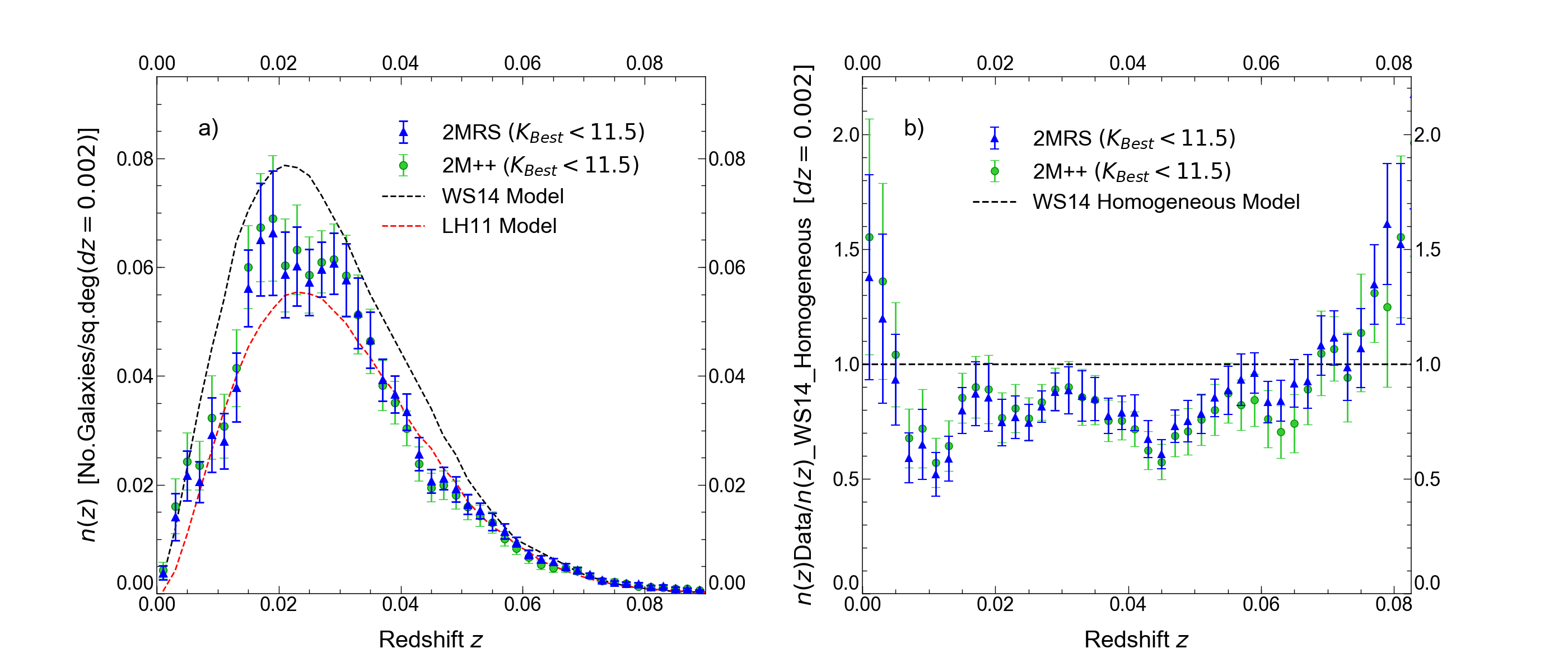
Figure 1: The observed $n(z)$ distributions of the 2MRS and 2M++ Catalogues measured to the wide-sky area $|b|\ga 5^{\circ}$, and consistently limited to $K<11.5$ where: (a) Counts are fit alongside the WS14 homogeneous model and LH11-normalised model over a bin size $\Delta z=0.002$. (b) The $n(z)$ counts are normalised to the WS14 model to demonstrate observed under- and overdensities across the distribution.

4 Galaxy redshift distribution

The observed $n(z)$ distribution measured in the 2MRS and 2M++ catalogues over the wide-sky area to $|b|\ga 5^{\circ}$ is shown in Fig. 1(a). The data are limited to $K<11.5$ and compared to the $n(z)$ predictions of the homogeneous WS14 LF model, with a corresponding plot of the observed $n(z)$ divided by the model shown in Fig. 1 (b). Counts have been corrected with the spectroscopic incompleteness factor described in Section 2.2.3, and a description of the completeness of each sample as a function of magnitude is given in Appendix D. Errors have been calculated using the field-field method incorporating the uncertainty in each observed redshift bin combined with the uncertainty in the incompleteness.

Subject to the limiting magnitude $K<11.5$, each survey shows a distribution where the majority of the observed $n(z)$ data fall below the predicted count of the WS14 homogeneous model. The observed distributions fail to converge to the model until $z>0.06$ and below this range the data exhibit a characteristic under-density that is consistent with $n(z)$ counts over the NGC and SGC presented in WS14.

To analyse the scale of under-density in our measurements, we consider the ‘total’ density contrast, calculated by evaluating the difference between the sum of the observed count and predicted count, normalised to the sum of the predicted count. Here we take the sum over $n(z)$ bins from $z=0$ to the upper limits of $z=0.05$ and $z=0.075$. Calculations of the density contrast in our wide-sky 2MRS and 2M++ distributions within these bounds are presented in Table 3.

Table 3: The measured density contrasts between the WS14 LF model and $n(z)$ counts of 2MRS and 2M++ over the $\sim 37,000$ sq. deg. wide-sky area. The samples are taken to a limiting magnitude $K<11.5$ and detail the scale of under- and overdensities to the specified ranges $z<0.05$ and $z<0.075$.

Sample Limit	Survey	Density Contrast $(\%)$
$z<0.05$	2MRS	$-23\pm 2$
	2M++	$-21\pm 3$
$z<0.075$	2MRS	$-22\pm 2$
	2M++	$-21\pm 2$

The measured density contrast of each survey at $z<0.075$ are in excellent agreement and indicate that the wide-sky $n(z)$ counts are $\sim 21-23\%$ underdense relative to the model. At both limits, the 2MRS dataset produces a marginally greater under-density than 2M++, however, the two values remain consistent to within $1\sigma$ and demonstrate a continuous under-density in the $n(z)$ distribution.

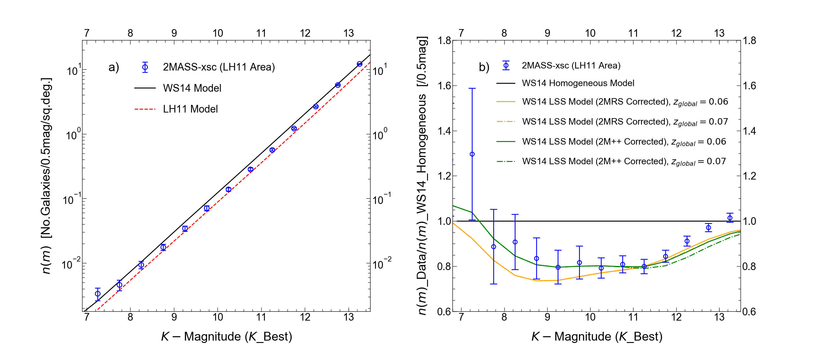
Figure 2: The observed $K-$band $n(m)$ counts of the 2MASS Extended Source Catalogue taken over the wide-sky region to $|b|\ga 5^{\circ}$, where: (a) The observed counts are compared to the WS14 and LH11 homogeneous models. (b) The observed counts divided by the WS14 homogeneous model are compared to the inhomogeneous, variable $\phi^{*}(z)$, versions of the WS14 models based on the 2MRS and 2M++ $n(z)$’s, and similarly divided by the homogeneous WS14 model. The transition to the homogeneous case for both of these inhomogeneous LSS models is investigated for both $z_{\text{global}}=0.06$ and $z_{\text{global}}=0.07$.

We note that in our approach we have applied a single incompleteness factor to correct each bin in the observed $n(z)$ distribution equally while a more detailed examination could incorporate a magnitude-dependent factor. This technique was implemented in WS14, where the completeness factor was introduced into the LF $n(z)$ model such that each bin conserved the galaxy number. However, the change to the $n(z)$ sample as a result of this method was less than $1\%$ and so we have not implemented this more detailed correction here.

We shall return in Section 6.1 to discuss the reasons for the difference in the $n(z)$ model prediction of Lavaux & Hudson (2011), also shown in Fig. 1(a).

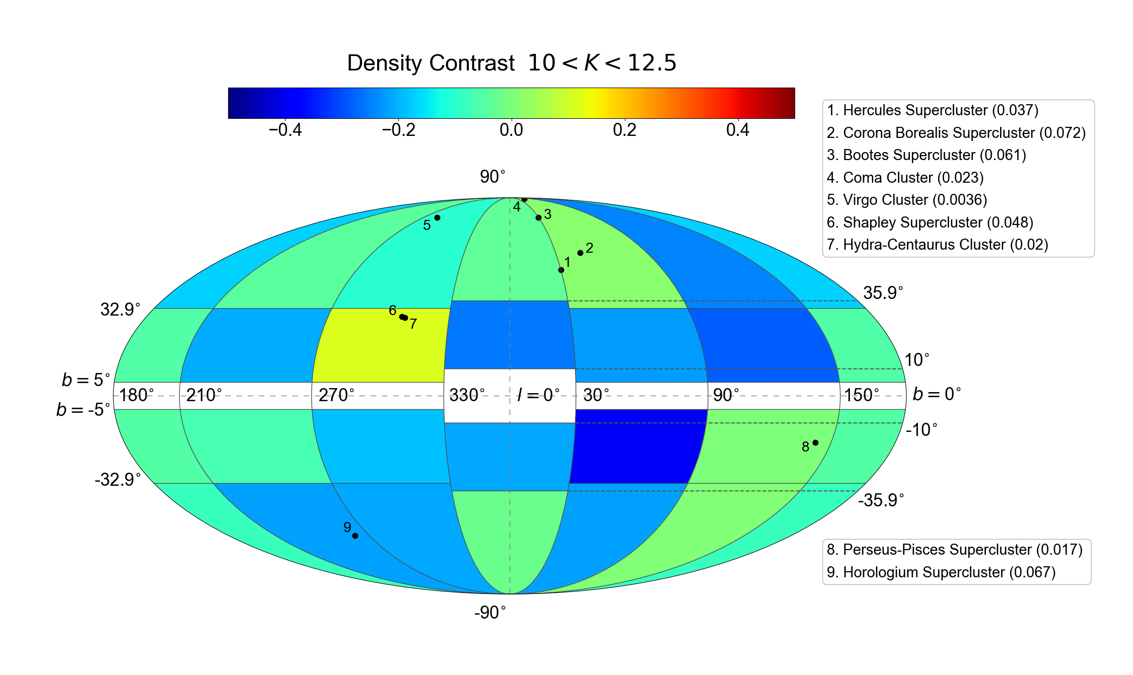
Figure 3: A Mollweide contour plot detailing the galactic coordinate positions of each sub-field we have used to calculate the field-field errors in our wide-sky $n(m)$ and $n(z)$ distributions. In each region we have evaluated the 2MASS $n(m)$ density contrast, measured at $10<K<12.5$, and plotted local galaxy structures to investigate the regional densities. The legend describes the key for each galaxy structure, and their corresponding redshift is given in brackets.

5 Galaxy number magnitude counts

5.1 2MASS $n(m)$ counts

We now consider the 2MASS number-magnitude counts, and examine the extent the WS14 homogeneous model can self-consistently replicate an $n(m)$ under-density that is of the same profile and at a similar depth as that suggested by the galaxy redshift distributions of 2MRS and 2M++.

The observed $K-$band $n(m)$ count of the 2MASS Extended Source Catalogue to the wide-sky limit of $|b|\ga 5^{\circ}$, is presented in Fig. 2(a). Similar to the $n(z)$ comparison in Fig. 1, these counts appear low compared to the homogeneous model of WS14, here at $K<12$.

To examine whether the $n(m)$ counts are consistent with the form of the under-density shown in the $n(z)$ measurements, we also predict this $n(m)$ based on the LSS-corrected $\phi^{*}(z)$ normalisation (see Section 3). We first show the observed $n(m)$ count divided by the homogeneous WS14 model in Fig 2(b). Then we use the $n(z)_{\text{obs}}$ derived from each of the 2MRS and 2M++ $n(z)$ distributions in Fig. 1 (b), both similarly divided by the WS14 homogeneous model. The orange and green lines represent the 2MRS and 2M++ -corrected models respectively.

At $K<12.5$, the wide-sky $n(m)$ distribution shows a significant under-density relative to the homogeneous prediction, only reaching consistency with the model at $K\approx 13$. Moreover, we find that the $\phi^{*}(z)$ models describing the observed $n(z)$ inhomogeneities in each of 2MRS and 2M++ give a significantly more accurate fit to the 2MASS $n(m)$ count. This indicates that the profile of the under-density in the galaxy redshift distributions, measured relative to the WS14 homogeneous prediction, is consistent with the observed $n(m)$ counts.

To explicitly evaluate the 2MASS $n(m)$ under-density, we give calculations of the density contrast in Table 4. To mitigate the uncertainty at the bright end and remain in line with measurements given by WS14, we take a fixed lower bound, $K>10$, and vary the upper magnitude bound.

Table 4: Measurements of the density contrast in the 2MASS wide-sky $n(m)$ counts relative to the WS14 model, taken to various $K-$ limits to examine the extent of underdensities in the distribution. Errors are field-field based on 24 sub-fields.

Sky Region	Sample Limit	Density Contrast ($\%$)
$|b|\ga 5^{\circ}$	$10<K<11.5$	$-20\pm 2$
$|b|\ga 5^{\circ}$	$10<K<12.5$	$-13\pm 1$
$|b|\ga 5^{\circ}$	$10<K<13.5$	$-3\pm 1$

The measurements of the total density contrast in the wide-sky $n(m)$ count in Table 4 demonstrate a significant scale of under-density at $10<K<11.5$ that becomes less pronounced approaching $K\approx 13.5$. Notably, at $K<11.5$ we measure an under-density of $20\pm 2\%$, which is consistent with the $\approx 21-22\%$ under-density shown in the 2MRS and 2M++ $n(z)$ counts. Additionally, for $K<12.5$ we find a wide-sky under-density of $13\pm 1\%$, which is in good agreement with the $15\pm 3\%$ under-density calculated in the three WS14 fields over the same magnitude range. The field-field errors suggest strongly significant detections of a 13-21% underdensity over the wide-sky area. This is in agreement with WS14, who found an $\approx 15$% underdensity from their sample covering a $\approx 4\times$ smaller area over the NGC and SGC. In addition, we note the effect of the magnitude calibration to the Loveday system. Excluding the correction lowers the observed count at the faint end by $\approx 10\%$, confirming the conclusion of WS14 that an under-density is seen independent of applying the Loveday magnitude correction. Finally, we again shall return in Section 6.1 to discuss why the $n(m)$ model prediction of LH11 also shown in Fig. 2(a) are so much lower than that of WS14.

5.2 Sub-field $n(m)$ Density Contrast Measurements

To further assess the sky extent of the Local Hole, we next consider the properties of the wide-sky sub-fields from which we derive the field-field errors and evaluate the 2MASS $n(m)$ density contrast in each sub-field region.

Fig. 3 shows the density contrast between the 2MASS $n(m)$ counts and the WS14 homogeneous model in each sub-field area that is also used to evaluate the wide-sky $n(m)$ and $n(z)$ field-field errors. The average density contrast in each field is plotted colour-coded on a Mollweide projection, which also details the geometric boundaries of each region in Galactic coordinates.

To probe the under-density, we choose to take the sum over the range $10<K<12.5$ to remain consistent with the limits considered in WS14. In addition, to examine the properties of individual regions we plot the local galaxy clusters and superclusters highlighted in LH11 using positional data from Abell et al. (1989), Einasto et al. (1997) and Ebeling et al. (1998), and provide their redshift as quoted by Huchra et al. (2012) in the 2MRS Catalogue.

From the lack of yellow-red colours in Fig. 3 it is clear that underdensities dominate the local Large Scale Structure across the sky. Now, there are several fields which demonstrate an $n(m)$ count that marginally exceeds the WS14 prediction and we find that such (light green) regions tend to host well known local galaxy clusters. The 4 out of 24 areas that show an over-density are those that contain clusters 2,3,4 - Corona Borealis+Bootes+Coma; 6,7 - Shapley+Hydra-Centaurus; 8 - Perseus-Pisces, using the numbering system from Fig. 3. The influence of the structures in these 4 areas is still not enough to dominate the Local Hole overall $13\pm 1$% under-density in the wide-sky area in Fig. 3.

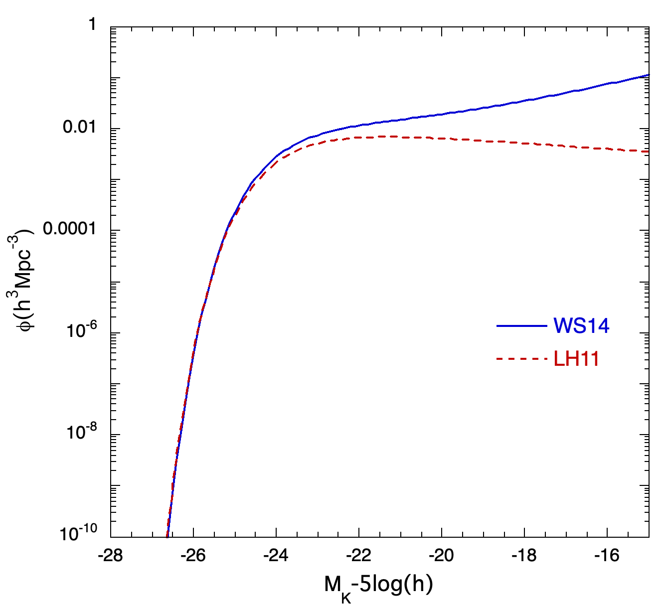
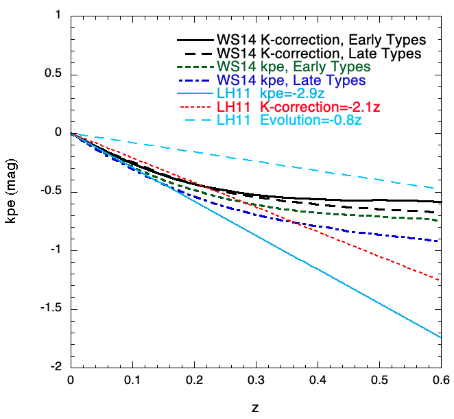
Figure 4: (a) The galaxy $K$ luminosity function of WS14 as used here compared to that of LH11. (b) The $k$ and $k+e$ corrections of WS14 compared to those of LH11, for the $K$-band.

We conclude that the observed $n(m)$ and $n(z)$ galaxy counts taken to $|b|\ga 5^{\circ}$ in 2MASS, 2MRS and 2M++, show a consistent overall under-density measured relative to the WS14 model that covers $\approx 90$% of the sky. At a limiting depth of $K=11.5$ the $n(m)$ counts show an under-density of $20\pm 2$% and this scale is replicated in form in the $K-$limited $n(z)$ distributions at $z<0.075$ which show an under-density of $\sim 21-22$%.

6 Comparison of LF and other model parameters

The above arguments for the Local Hole under-density depend on the accuracy of our model LF and to a lesser extent our $k+e$ parameters that are the basis of our $n(z)$ and $n(m)$ models. We note that Whitbourn & Shanks (2016) made several different estimates of the galaxy LF in the $K$ band from the $K<12.5$ 6dF and SDSS redshift surveys including parametric and non-parametric ‘cluster-free’ estimators and found good agreement with the form of the LF used by WS14 and in this work. The ‘cluster-free’ methods are required since they ensure that at least the form of the LF is independent of the local large-scale structure and mitigates the presence of voids as well as clusters. The non-parametric estimators also allowed independent estimates of the local galaxy density profiles to be made and showed that the results of WS14 were robust in terms of the choice of LF model. The WS14 LF normalisation was also tested using various methods as described in Section 2.3.1 of Whitbourn & Shanks (2016).

We now turn to a comparison between the WS14 galaxy count predictions with those made by Lavaux & Hudson (2011) who failed to find an under-density in the 2M++ $n(z)$ data. To examine the counts produced by their model we assume the LF parameters given in their Table 2, where in the Local Group frame with $750<v<20000$ km s^-1, they find $\alpha=-0.86$; $M^{*}=-23.24+5{\rm log}_{10}(h)$; $\phi^{*}=1.13\times 10^{-2}h^{3}{\rm Mpc}^{-3}$, independent of galaxy type. Note that we brighten the LH11 $M^{*}$ by 0.19 mag to $M^{*}=-23.43+5{\rm log}_{10}(h)$ in our version of their model to account for the 0.19 mag difference between $K\_m\_ext$ magnitudes used here and the 2MASS $K_{Kron}(=K\_20)$ magnitudes used by LH11 (see Appendix B). In Fig. 4 (a) we compare their $z=0$ LF with our LF summed over our five galaxy types. Importantly, LH11 note that their fitted LFs show a distinctly flatter faint slope ($\alpha>-1$) than other low redshift LF estimates (see their Fig 7a) that generally look more similar to the steeper WS14 LF (see also Whitbourn & Shanks 2016). However, Fig. 4 (a) shows that the form of both LF’s is similar in the range around $M^{*}$ that dominates in magnitude limited galaxy samples, apart from their normalisation, with the LH11 LF appearing $\approx 40$% lower than that of WS14. We shall argue that this low normalisation is crucial in the failure of LH11 to find the ‘Local Hole’.

Next, we compare the $k+e$ - redshift models of LH11 and WS14 in Fig. 4b. Two $k+e(z)$ models are shown for WS14 representing their early-type model applied to E/S0/Sab and their late type model applied to Sbc/Scd/Sdm. These models come from Bruzual & Charlot (2003) with parameters as described by Metcalfe et al. (2006) At $z=0.1$ these models give respectively $\Delta_{K}=-0.28$ and $\Delta_{K}=-0.31$. We also show just the $k(z)$ for early and late types in Fig.4. At $z=0.1$ these $k(z)$ models give respectively $\Delta_{K}=-0.26$ and $\Delta_{K}=-0.25$, implying little evolution in the $e(z)$ model for the early types and 0.06 mag for the late types.

We note that LH11 apply their $k+e$ corrections to the data whereas we apply them to the model. So reversing their sign on their $k(z)$ and $e(z)$ terms, the correction we add to our $K$ magnitudes in our count model is

$$\Delta_{K}(z)=k(z)-e(z).$$ (7)

LH11 give $k(z)=-2.1z$ and $e(z)=0.8z$ giving our additive correction as

$$\Delta_{K}(z)=k(z)-e(z)=-2.1z-0.8z=-2.9z$$ (8)

as representing the LH11 $k$- and evolutionary corrections, giving $\Delta_{K}=-0.29$mag at $z=0.1$. Their second model includes an additional galaxy $(1+z)^{4}$ surface brightness dimming correction so in magnitudes is

$$\Delta_{K}(z)=0.16(10\log_{10}(1+z))+1.16(k(z)-e(z))$$ (9)

i.e.

$$\Delta_{K}(z)=1.6\log_{10}(1+z)-3.4z$$ (10)

and so $\Delta_{K}=-0.27$mag at $z=0.1$.

Since we are using total $K$ magnitudes, the effect of cosmological dimming of surface brightness is included in our measured magnitudes. So in any comparison of the LH11 model with our $K$ band data, only the $k+e$ terms are used in the model. So at $z=0.1$ our $k+e$ term is $\Delta_{K}\approx-0.29$mag, the same as the $\Delta_{K}=-0.29$mag of LH11. Similarly at $z=0.3$ which is effectively our largest redshift of interest at $K<15.5$, $z=0.3$, $\Delta_{K}\approx-0.60$ to -0.69 mag for the WS14 $k+e$ model compared to $\Delta_{K}=-0.87$mag for LH11.

6.1 Lavaux & Hudson $n(m)$ and $n(z)$ comparisons to $K=11.5$

In Figs. 1(a) and  2(a) we now compare the LH11 model predictions to those of WS14 for the 2MRS and 2M++ $n(z)$ and 2MASS $n(K)$ distributions. Most notably, we find that the LH11 model produces theoretical $n(K)$ and $n(z)$ counts that are significantly lower than the WS14 counterparts and, if anything, slightly under-predict the observed wide-sky counts particularly near the peak of the $n(z)$ in Fig. 1(a). The LH11 $n(K)$ model is offset by $\approx 40$% from the WS14 $n(K)$ prediction. We also note that the $n(z)$ distribution predicted by LH11 when compared to the 2M++ $n(z)$, limited at $K=11.5/12.5$ mag, shows excellent agreement (see LH11 Fig. 5). However, in Fig. 2(a), beyond $K>12.5$, the LH11 $n(K)$ model diverges away from the 2MASS data. In contrast, the WS14 model was found to generate a consistency between the wide-sky $n(K)$ and $n(z)$ distributions and imply a similar under-density of $\approx 20$% at $K<11.5$. Due to the consistency of the slope in each model at both the bright and faint end of $n(K)$ counts, it is likely that the difference between the LH11 and the WS14 models is caused by the different effective normalisation in $\phi^{*}$ seen around the break in the LF in Fig. 4.

We further note that when we try to reproduce Fig. 5 of LH11, by combining $n(z)$ model predictions using their LF model parameters for their combined $K<11.5$ and $K<12.5$ 2M++ samples covering 13069 and 24011 deg² respectively, we find that we reasonably reproduce the form and normalisation of their predicted $n(z)$ to a few percent accuracy. So why the fit of the LH11 model is poorer than in our Fig. 1 (a) than in their Fig. 5 remains unknown. Nevertheless, we accept that their model fits our Fig. 1 (a) $n(z)$ better than the model of WS14.

6.2 Lavaux & Hudson $n(m)$ comparison at $K<16$

To examine the ability of the LH11 model simultaneously to predict the galaxy $n(K)$ at bright and faint magnitudes, we now compare the LH11 and WS14 models to the fainter $n(K)$ counts of the GAMA survey, shown in Fig. 5. We calculate errors using field-field errors as described in Section 2.3.

To compare the count models, we again assume the LH11 LF parameters from their Table 2, $\alpha=-0.86$; $M^{*}=-23.24+5{\rm log}_{10}(h)$ (corrected brighter by 0.19 mag into our system); $\phi^{*}=1.13\times 10^{-2}h^{3}{\rm Mpc}^{-3}$. We also assume the $k+e$ term of $\Delta_{K}=-2.9z$ used by LH11, one cut at $z<0.6$ and one cut at $z<1$ as shown by the dashed and dotted lines in Fig. 5.

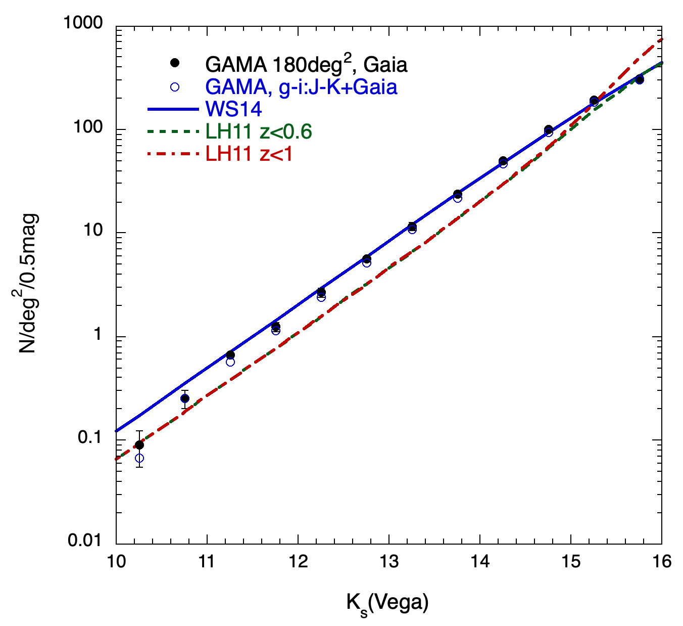
Figure 5: The WS14 and LH11 count models compared to the GAMA survey observed $n(K)$ counts averaged over 3 fields. Solid circles are the GAMA counts with the Gaia star-galaxy separation and open circles are with the Gaia separation applied after star-galaxy separating by colour (Baldry et al., 2010). Two versions of the LH11 model are shown with redshift cuts at $z<0.6$ and $z<1.0$ to prevent the model diverging due to an unphysical high redshift tail. Field-field errors based on the 3 GAMA fields are shown.

The two LH11 predictions reasonably fit the bright data at $K<11$ but lie below the observed GAMA data out to $K\approx 15$, then agreeing with these data at $K\approx 15.5$. In the case of the version cut at $z<1.0$, the model then rises above the GAMA counts. The model cut at $z<0.6$ remains in better agreement with these data. But without the redshift cuts we find that the $\Delta K=-2.9z$ k+e term used by LH11 would vastly overpredict the observed galaxy count not just at $K>15.5$mag but at brighter magnitudes too. This is the usual problem with an evolutionary explanation of the steep count slope at $K<12$, in that models that fits that slope then invariably overpredict the slope at fainter magnitudes. For an evolutionary model to fit, a strong evolution, either in galaxy density or luminosity (as in the LH11 + WS14 models used here) is needed out to $z<0.1$ and then something quite close to a no-evolution model is required at $0.1<z<1$ in the $K$ band. This is similar to what was found in the $b_{J}$-band where strong luminosity evolution is at least more plausible. In $K$ the evolution is less affected by increasing numbers of young blue stars with redshift and so the evolutionary explanation is even less attractive.

The conclusion that the steep $K$ counts are caused by local large-scale structure rather than evolution is strongly supported by the form of the $n(z)$ seen in Fig. 1 where the pattern of underdensities is quite irregular as expected if dominated by galaxy clustering rather than the smoothly increasing count with $z$ expected from evolution. We have also shown that following the detailed changes in $n(z)$ with redshift to model $\phi^{*}(z)$ gives a consistent fit to the steep $n(m)$ distribution at $K<12$. We conclude that unless a galaxy evolution model appears that has the required quick cut-off at $z\approx 0.1$ required simultaneously in the $K$ and $b_{J}$ counts then the simplest explanation of the steep $n(K)$ slope at bright magnitudes is the large scale structure we have termed the ‘Local Hole‘.

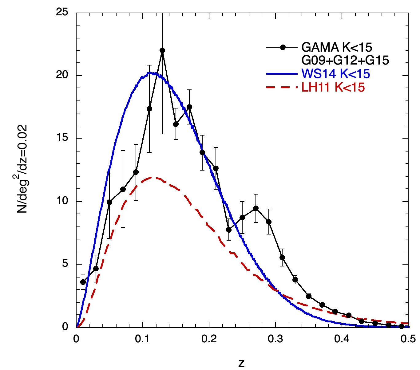
Figure 6: Galaxy $n(z)$ for GAMA survey limited at $10<K<15$ and the predictions of the WS14 and LH11 models. We chose the $K<15$ limit here because this appears to be the effective limit for the $K$ band spectroscopic survey in G09 and G12, although G15 may be complete to a 0.5mag fainter limit. We note that there is a ‘bump’ in the GAMA $n(z)$ at $z\approx 0.25$ that appears to have its origin mostly in the G09 and G15 fields with less contribution from G12. G09 and G15 are the two most widely separated fields of the three, arguing that this feature is a statistical fluctuation, if not caused by some $z$ survey target selection issue.

These conclusions are confirmed by the GAMA $n(z)$ in the range $10<K<15$, averaged over the G09, G12 and G15 fields and compared to the WS14 + LH11 models in Fig. 6. Similar results are seen to those for the GAMA $n(K)$ in Fig. 5 with the WS14 model better fitting these data than the LH11 model that again significantly underestimates the observed $n(z)$. Some hint of an under-density is seen out to $z\approx 0.12$ in the WS14 model comparison with the observed data but the area covered is only $180$ deg² so the statistical errors are much larger than for the brighter $K<11.5$ or $K<12.5$ ‘wide-sky’ redshift survey samples.

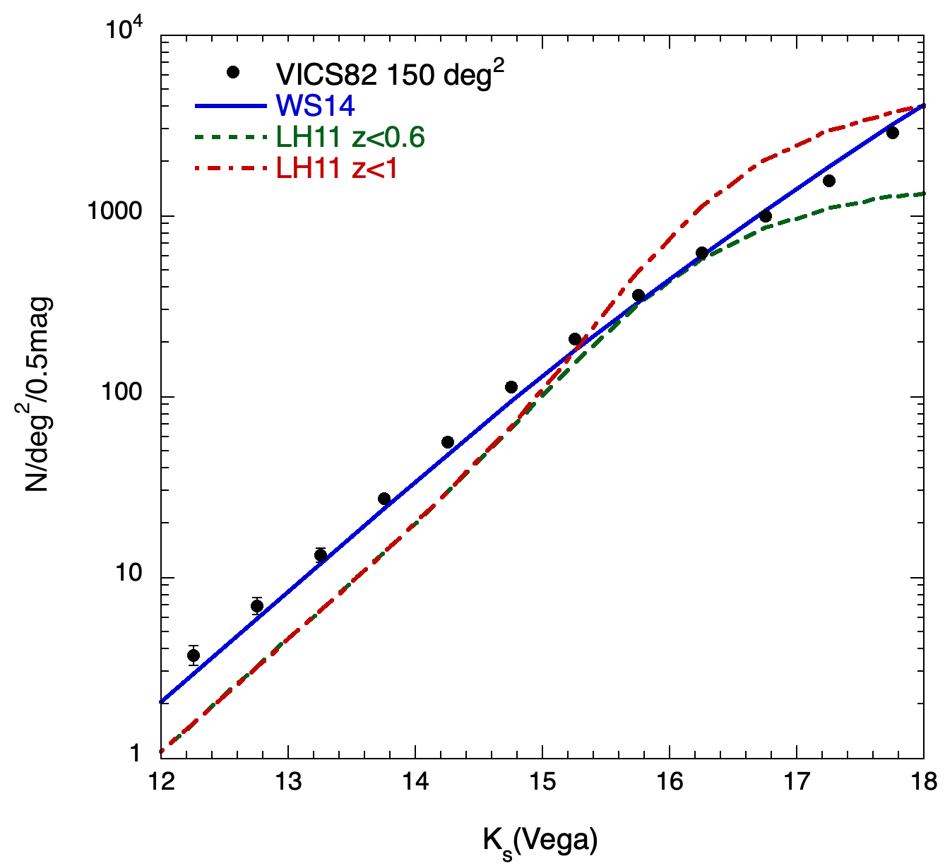
Figure 7: The WS14 and LH11 count models compared to the VICS82 survey (Geach et al., 2017) observed $n(K)$ counts averaged over $\approx 150$ deg² to $K<18$. Results are based on star-galaxy separation $Class\_Star<0.9$ with further removal of Gaia pointlike objects as defined by eq 3. Field-field errors based on 2 sub-fields of area 69 and 81 deg² are shown. The LH11 models again have redshift cuts at $z<0.6$ and $z<1$ to prevent divergence due to an unphysical high redshift tail.

6.3 VICS82 $K$ count model comparison to $K=18$

To assess further the LF normalisation uncertainties, we present in Fig. 7 the $n(K)$ galaxy counts in the range $12<K<18$ over the $\approx 150$deg² area of the VICS82 survey (Geach et al., 2017). Here, the faint $K=18$ limit is 2 mag fainter than the GAMA limit in Fig. 5. Use of the fainter, $K>18$, VICS82 data to test LF parameters would increasingly depend on the evolutionary model assumed. The bright limit is chosen because the $Class~{}Star$ parameter is only calculated by Geach et al. (2017) for $K>12$ to avoid effects of saturation. The $K$ magnitudes are corrected into the 2MASS $K\_m\_ext$ system (see Section 2.1.3 and Appendix C). As also described in Section 2.1.3 we have assumed a conservative star-galaxy separation using $Class~{}Star<0.9$ and then removing any remaining pointlike objects using Gaia data and eq 3. We note that there is good agreement with the counts given by Geach et al. (2017) in their Fig. 5, once our magnitude offsets are taken into account. In the full range, $12<K<16$, we again see excellent agreement with the WS14 model and again the LH11 model significantly under-predicts the galaxy counts. We conclude that, like the GAMA counts, the VICS82 $K$-band data also strongly support the accuracy of the WS14 model and its LF parameters, from counts based on a completely independent sky area.

6.4 Discussion

What we observe is that the brighter $K<11.5$ 2MRS $n(z)$ requires a 20% lower $\phi^{*}$ than the $K<15$ GAMA $n(z)$. So good fits to both $n(z)$’s can be obtained if the LF $\phi^{*}$ is left as a free parameter (see also Fig. 7 of Sedgwick et al. 2021). This means that the Local Hole may have quite a sharp spatial edge at $z\approx 0.08$ or $r\approx 240h^{-1}$ Mpc. Otherwise, in an evolutionary interpretation this would look more like pure density evolution than luminosity evolution. In the density evolution case it is true that it would be nearly impossible to differentiate a physical under-density from a smoothly increasing galaxy density with redshift due to evolution. But the reasonable fit of homogeneous models in the $z<0.08$ range would again imply that there was a sharp jump in the galaxy density above this redshift. Again this increase in density cannot continue at $z>0.08$ for the same reason as for pure luminosity evolution, since the counts at higher redshift would quickly be over-predicted. We regard either of these sharply changing evolutionary scenarios around $z\approx 0.08$ as much less likely than an under-density, as has been argued for some years even on the basis of blue-band number counts (Shanks, 1990; Metcalfe et al., 1991).

We highlight the relative normalisations of the WS14 and LH11 LF models as the key outcome of our analysis. The LH11 model fails to fit the faint $n(m)$ galaxy counts in the GAMA survey. If their normalisation is correct and no local under-density exists then it is implied that galaxies must evolve in a way that their space density sharply increases at $z\ga 0.08$ and $K>12$ and then returns to a non-evolving form out to $z\approx 0.5$ and $K>20$. This single spurt of evolution at $z\approx 0.08$ has to be seen at similar levels in the $b_{J}$, $r$ and $H$ bands as well as in the $K$ band. It was the unnaturalness of this evolutionary interpretation that originally led e.g. Shanks (1990) to normalise their LF estimates at $b_{J}(\sim g)>17$ mag rather than at brighter magnitudes where the form of the LF was estimated. Even authors who originally suggested such an evolutionary explanation (e.g. Maddox et al. 1990) have more recently suggested that a large scale structure explanation was more plausible (e.g. Norberg et al. 2002). Moreover, WS14 have presented dynamical evidence for a local outflow in their analysis of the relation between $\bar{z}$ and $m$ and Shanks et al. (2019a); Shanks et al. (2019b) have shown that this outflow is consistent with the Local Hole under-density proposed here. It will also be interesting to see whether future all-sky SNIa supernova surveys confirm this $\bar{z}:m$ outflow evidence, based as it is on the assumption that the $K-$band luminosity function is a reasonable standard candle.

We suggest that the crucial issue for LH11 and Sedgwick et al. (2021) is that they have fitted their LF parameters and particularly the LF normalisation in the volume dominated by the Local Hole and thus calibrated out the under-density. Certainly their $n(K)$ and $n(z)$ models clearly fail at magnitudes and redshifts just outside the ranges where they have determined their LF parameters. These authors would need to show powerful evidence for the $z<0.1$ evolution spurt in the favoured $\Lambda$CDM model before their rejection of the Local Hole hypothesis could be accepted. In the absence of such a model the balance of evidence will clearly favour the Local Hole hypothesis.

7 Conclusions

In this work we have examined the local galaxy distribution and extended the work of Whitbourn & Shanks (2014) by measuring observed number-redshift $n(z)$ and number-magnitude $n(m)$ galaxy counts in the $K-$band across $\approx 90$% of the sky down to a Galactic latitude $|b|\ga 5^{\circ}$.

The $n(z)$ distributions from the 2MRS and 2M++ surveys to $K<11.5$ were compared to the homogeneous model of WS14 (see also Metcalfe et al. 2001, 2006). These wide-sky $n(z)$ distributions showed excellent agreement and implied an under-density of $22\pm 2$% relative to the model at $z<0.075$. We also find that the 2MASS $K$ counts show a similar under-density of $20\pm 2\%$ at $K<11.5$ relative to the same model, only converging to the predicted count at $K\approx 13.5$. In addition, an LSS-corrected $\phi^{*}(z)$ model based on the $n(z)$ distribution, when compared to the 2MASS $K$ counts, showed a much improved fit, confirming the consistency of the 2MASS $n(m)$ and the 2MRS/2M++ $n(z)$ in detecting this under-density relative to the WS14 model. We also found the under-density covered 20/24 or $\approx 83$% of the observable wide-sky with only areas containing the Shapley and other super-clusters and rich clusters like Coma showing up as over- rather than an under-densities.

Combined, our $n(m)$ and $n(z)$ counts are in good agreement with the work of WS14, Frith et al. (2003), Busswell et al. (2004) and Keenan et al. (2013), who find overall underdensities of the order $\approx 15-25$ % using a similar galaxy counts method. We also recall that in the $\approx 9000$deg² sky area analysed by WS14, the under-density patterns found in redshift were confirmed in detail by the distribution traced by X-ray galaxy clusters in the same volume (Böhringer et al., 2020).

To examine whether our measured under-density represents a physical Local Hole in the galaxy environment around our observer location requires a confirmation of the accuracy of the WS14 galaxy count model. We have investigated this by comparing the model’s predictions for the fainter $K$ galaxy counts from the GAMA and VICS82 surveys. We have also compared these data with the model predictions of LH11 who failed to find an under-density in the 2M++ survey.

The $n(m)$ and $n(z)$ counts predicted by the LH11 model are lower by $\approx 40$% compared to the WS14 model; the LH11 model thus initially appears to under-predict the observed wide-sky $n(K)$ and $n(z)$ distributions from 2MASS, 2MRS and 2M++. Then, at $K>13.5$, beyond the 2MASS sample range, the WS14 prediction fits very well the observed $n(K)$ and $n(z)$ counts in the GAMA survey and the observed $n(K)$ in the VICS82 survey. However, the LH11 model shows a consistently poor fit over both the full GAMA+VICS82 $n(K)$ and GAMA $n(z)$ distributions. Thus the GAMA + VICS82 results indicate that the WS14 model can more accurately fit deep $K-$ counts than the LH11 model, supporting its use in interpreting the lower redshift, wide-sky surveys.

Consequently, our analyses here support the existence of the ‘Local Hole’ under-density over $\approx 90$% of the sky. At the limiting magnitude $K<11.5$ the under-density of $20\pm 2$% in the $n(z)$ counts corresponds to a depth of $\approx 100h^{-1}$ Mpc, while the $13\pm 1$% under-density at $K<12.5$ in the 2MASS wide-sky $n(m)$ counts, that is in good agreement with WS14, would imply the under-density extends further to a depth of $\approx 150h^{-1}$Mpc. We note that the statistical error on our LF normalisation can be easily estimated from the field-to-field errors in the $10<K<15$ galaxy counts between the 3 GAMA fields (see Table 5) and this gives an error of $\pm 3.4$%. The error estimated from the two VICS82 sub-fields would be similar at $\pm 3.6$% in the range $12<K<16$, decreasing to $\pm 1.1$% in the range $12<K<18$. Combining the GAMA $\pm 3.4$% error with the $\pm 2$% error on the -20% under-density to $K<11.5$ mag gives the full uncertainty on the Local Hole under-density out to 100h^-1 Mpc to be $-20\pm 3.9$% i.e. a $5.1\sigma$ detection. Similarly the Local Hole $K<12.5$ under-density out to $\approx 150$h^-1 Mpc is a $-13\pm 3.5$% or a $3.7\sigma$ detection.

Such a 13-20% underdensity at $\approx$100-150 h^-1Mpc scales would notably affect distance scale measurements of the expansion rate $H_{0}$. We can calculate this by assuming the linear theory discussed in WS14 and Shanks et al. (2019a), where $\delta H_{0}/H_{0}=-\frac{1}{3}\,\delta\rho_{g}/\rho_{g}\times\Omega_{m}^{0.6}/b$. Here we take the galaxy bias $b\approx 1.2$ for $K-$selected 2MRS galaxies in the standard model (see e.g. Boruah et al. 2020; also Maller et al. 2005; Frith et al. 2005b although these latter $b$ values should be treated as upper limits since they apply to $K<13.5$ and bias is expected to rise with redshift.) From our measured $n(m)$ and $n(z)$ underdensities this would produce a decrease in the local value of $H_{0}$ of $\approx 2-3$%.

We finally consider the significance of such a large scale inhomogeneity within the standard cosmological model. Frith et al. (2006) created mock 2MASS catalogues from the Hubble Volume simulation to determine theoretically allowed fluctuations and found that a $1\sigma$ fluctuation to $H=13$ ($K\approx 12.5$) over 65% of the sky corresponded to $\pm 3.25$%. Scaling this to the 90% wide-sky coverage used here implies $1\sigma=2.8$%. Given our $13\pm 3.5$% under-density to $K<12.5$, we can add in quadrature this $\pm 2.8$% expected fluctuation from the $\Lambda$CDM model to obtain $13\pm 4.5$% with the error now including our measurement error and the expected count fluctuation expected out to $\approx 150$h^-1 in $\Lambda$CDM. The Local Hole with a 13% under-density therefore here corresponds to a $2.9\sigma$ deviation from what is expected in a $\Lambda$CDM cosmology.

If we scale this from $K<12.5$ mag to $K<11.5$ mag via a 3-D version of Eq. 3 of Frith et al. (2005a), a $1\sigma$ fluctuation at $K<11.5$ corresponds to $\pm 5.6$%. At $K<12.5$, the under-density is $-20\pm 2$% and folding in the $\pm 3.4$% normalisation error gives $-20\pm 3.9$% or a $5.1\sigma$ detection of the Local Hole under-density. Then adding in the $\pm 5.6$% expected fluctuation amplitude just calculated gives $-20\pm 6.8$%, implying again a $2.9\sigma$ deviation in the $\Lambda$CDM cosmology, similar to the $K<11.5$ case.

However, the deviation from $\Lambda$CDM is likely to be more significant. For example, if we normalised our model via the VICS82 $n(K)$ counts in the $12<K<18$ range (see Fig. 7) then this would argue that our LF normalisation should be still higher and the field-field error would also be lower at $\pm 1.1$%. Additionally, taking into account the excellent fit of the WS14 model to the 2MASS wide-sky data itself at $12.5<K<13.5$ (see Fig. 2) would also further increase the significance of the deviation from $\Lambda$CDM.

Although the Hubble Volume mocks of Frith et al. (2006) have tested our methodology in the context of an N-body simulation ‘snapshot’ with an appropriate galaxy clustering amplitude in volumes similar to those sampled here, it would be useful to make further tests in a more realistic simulation. For example, a full lightcone analysis could be made, applying our selection cuts in a mock that includes a full ‘semi-analytic’ galaxy formation model (e.g. Sawala et al. 2022). This would make a further direct test of our methodology while checking if there is any evolutionary effect that provides the spurt of density evolution at $z\approx 0.08$ required to provide an alternative to our large-scale clustering explanation of the Local Hole.

We therefore anticipate that further work to separate out the effects of evolution and LSS on the luminosity function in each of the WS14 and LH11 approaches will shed further light on the presence and extent of the Local Hole. Similarly, further work will be needed to resolve the discrepancy between the detection of dynamical infall at the appropriate level implied from the Local Hole under-density found by WS14, Shanks et al. (2019a) and Shanks et al. (2019b) as compared to the lack of such infall found by Kenworthy et al. (2019) and Sedgwick et al. (2021). But here we have confirmed that the proposed Local Hole under-density extends to cover almost the whole sky, and argued that previous failures to find the under-density are generally due to homogeneous number count models that assume global LF normalisations that are biased low by being determined within the Local Hole region itself.

Finally, if the form of the galaxy $n(K)$ and $n(z)$ do imply a ‘Local Hole’ then how could it fit into the standard $\Lambda$CDM cosmology? Other authors have suggested possibilities to explain unexpectedly large scale inhomogeneities such as an anisotropic Universe (e.g. Secrest et al. 2021). However, it is hard to see how such suggestions retain the successes of the standard model in terms of the CMB power spectrum etc. We note that other anomalies in the local galaxy distribution exist e.g. Mackenzie et al. (2017) presented evidence for a coherence in the galaxy redshift distribution across $\approx 600$h^-1 Mpc of the Southern sky out to $z\approx 0.1$. Prompted by this result and by the ‘Local Hole’ result reported here, Callow et al. (2021, in prep.) will discuss the possibilities that arise if the topology of the Universe is not simply connected. We emphasise that there is no proof but here we just use this model as an example of one that might retain the basic features of the standard model while producing a larger than expected coherent local under- or over-density. It will be interesting to look for other models that introduce such ‘new physics‘ to explain the local large-scale structure while simultaneously reducing the tension in Hubble’s Constant.

Data Availability

The 2MASS, 2MRS, 6dF, SDSS, GAMA, VICS82 and Gaia data we have used are all publicly available. All other data relevant to this publication will be supplied on request to the authors.

Appendix A GAMA-2MASS magnitude comparison

We first show Fig. 8 where GAMA MAG_AUTO_K and 2MASS $K\_m\_ext$ magnitudes are directly compared. Table 5 shows the error weighted mean of the differences between these two for each GAMA field within the range $10<K\_GAMA<13.5$ mag. Similarly Fig. 9 shows the comparison between GAMA MAG_AUTO_K and 2MASS magnitudes and Table 5 again shows the error weighted mean of the differences for each field in the same $K\_GAMA$ range

Following WS14, we have conservatively corrected the GAMA magnitudes for each of the three fields by correcting the GAMA magnitudes by adding the 2MASS $K\_m\_ext$ magnitude offsets given in the fourth column of Table 5 rather than the 2MASS $k\_BEST$ offsets given in the third column. This takes the GAMA magnitudes into the 2MASS $K\_m\_ext$ system rather than the $K\_BEST$ system we are actually using. Clearly if we used the $K\_BEST$ offsets the GAMA $K$ counts would lie even higher in Fig. 5.

Table 5: The magnitude offsets needed to correct the GAMA MAG_AUTO_K ($=K\_GAMA$) in each of the GAMA fields into the 2MASS $K\_BEST$ and $K\_m\_ext$ systems. They were calculated by taking an error weighted mean of the magnitude differences in $10<K_{GAMA}<13.5$ mag.

GAMA	N (2MASS	Weighted Mean	Weighted Mean
Field	$\times$GAMA)	$K_{Best}-K_{GAMA}$	$K\_m\_ext-K_{GAMA}$
G09	876	$0.019\pm 0.004$	$0.071\pm 0.004$
G12	1,208	$-0.011\pm 0.003$	$0.039\pm 0.004$
G15	1,184	$-0.017\pm 0.004$	$0.033\pm 0.004$

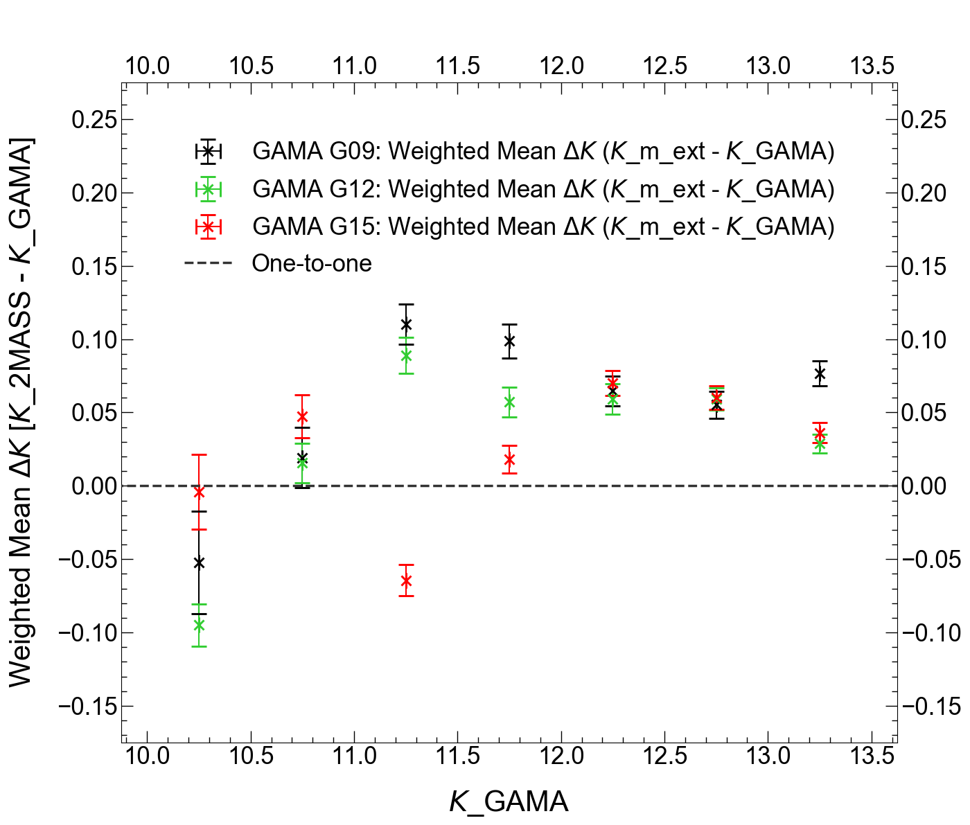
Figure 8: Differences between 2MASS $K\_m\_ext$ and GAMA MAG_AUTO_K as a function of GAMA magnitudes for each GAMA field.

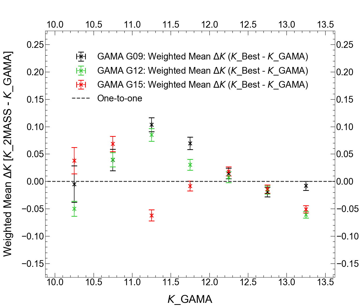
Figure 9: Differences between 2MASS $K\_BEST$ and GAMA MAG_AUTO_K as a function of GAMA magnitudes

Appendix B 2MASS magnitude comparison

Here we compare the 2MASS magnitude system, $K\_m\_ext$, on which our and WS14 $n(K)$ results are based with the 2MASS $K\_20(=K\_Kron)$ magnitudes used by LH11. The comparisons are shown as a function of $K\_m\_ext$ in Table 6 and Fig. 10. The overall difference is found to be $K\_m\_ext-K\_20=0.19\pm 0.0002$ mag.

Table 6: The 2MASS magnitude offsets between the $K\_m\_ext$ magnitudes on which WS14 and our magnitudes are based and the $K\_20$ magnitudes used by LH11 (see Fig. 10).

Magnitude Range	$N_{gal}$	Weighted Mean
	2MASS	$K\_m\_ext-K\_20$
$10.0<K\_m\_ext<10.5$	4,859	$0.139\pm 0.0008$
$10.5<K\_m\_ext<11.0$	9,827	$0.156\pm 0.0007$
$11.0<K\_m\_ext<11.5$	18,846	$0.166\pm 0.0006$
$11.5<K\_m\_ext<12.0$	38,756	$0.171\pm 0.0005$
$12.0<K\_m\_ext<12.5$	81,227	$0.184\pm 0.0004$
$12.5<K\_m\_ext<13.0$	169,857	$0.198\pm 0.0004$
$13.0<K\_m\_ext<13.5$	359,686	$0.208\pm 0.0003$
$10.0<K\_m\_ext<13.5$	683,958	$0.188\pm 0.0002$

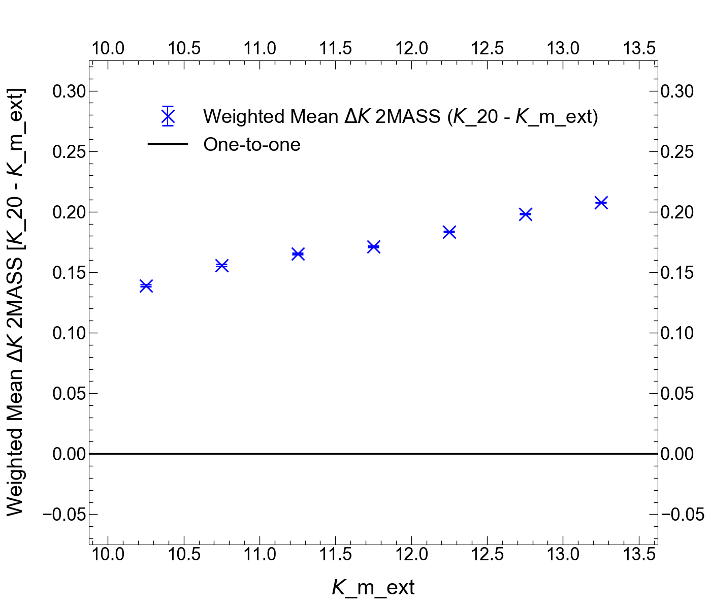
Figure 10: The 2MASS magnitude offsets from Table 6 between the $K\_m\_ext$ magnitudes on which WS14 and our magnitudes are based and the $K\_20$ magnitudes used by LH11.

Appendix C 2MASS-VICS82 magnitude comparison

Table 7 and Fig. 11 shows the offsets between] the $K\_m\_ext$ and VICS82 $MAG\_AUTO$ magnitude systems. Because of the possibility of saturation affecting the VICS82 magnitudes at $K<12.5$ and poor S/N affecting the fainter 2MASS magnitudes we simply average the 3 values in the range $12.5<K\_m\_ext<13.5$ to obtain the overall offset $K\_m\_ext-K\_VICS82=0.040\pm 0.004$ mag as used in Section 2.1.3.

Table 7: The offsets between the 2MASS $K\_m\_ext$ magnitudes on which WS14 and our magnitudes are based and the VICS82 $MAG\_AUTO$ magnitudes used by Geach et al. (2017) (see Fig. 11).

Magnitude Range	$N_{gal}$	Weighted Mean
	2MASS$\times$VICS82	$K\_m\_ext-K\_VICS82$
$10.0<K\_m\_ext<10.5$	26	$0.087\pm 0.007$
$10.5<K\_m\_ext<11.0$	31	$0.023\pm 0.009$
$11.0<K\_m\_ext<11.5$	73	$0.036\pm 0.007$
$11.5<K\_m\_ext<12.0$	175	$0.075\pm 0.005$
$12.0<K\_m\_ext<12.5$	361	$0.067\pm 0.005$
$12.5<K\_m\_ext<13.0$	730	$0.040\pm 0.004$
$13.0<K\_m\_ext<13.5$	1536	$0.013\pm 0.004$
$10.0<K\_m\_ext<13.5$	2932	$0.044\pm 0.002$

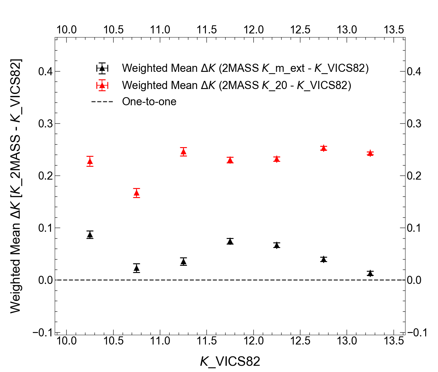
Figure 11: The offsets between the 2MASS $K\_m\_ext$ magnitudes on which WS14 and our magnitudes are based and the VICS82 $MAG\_AUTO$ magnitudes used by Geach et al. (2017) (see Table 7).

Appendix D Spectroscopic Incompleteness of $n(z)$ Counts

In Fig. 12 we present the calculation of the spectroscopic incompleteness factors applied to 2MRS and 2M++ $n(z)$ data before fitting to the WS14 homogeneous model. The $n(z)$ samples are matched to the 2MASS Extended Source Catalogue, and we plot the ratio of the $n(z)$ galaxy count to the 2MASS galaxy count, per half magnitude bin.

The overall completeness of each survey is calculated by the total sum of spectroscopic sources in either 2MRS or 2M++, divided by the total sum of photometric sources in 2MASS taken over the full magnitude range. We measure a completeness of $95\%$ in 2MRS and $88\%$ in 2M++, and the reciprocal of these values is the spectroscopic incompleteness factor which is multiplied to the raw $n(z)$ data of each survey.

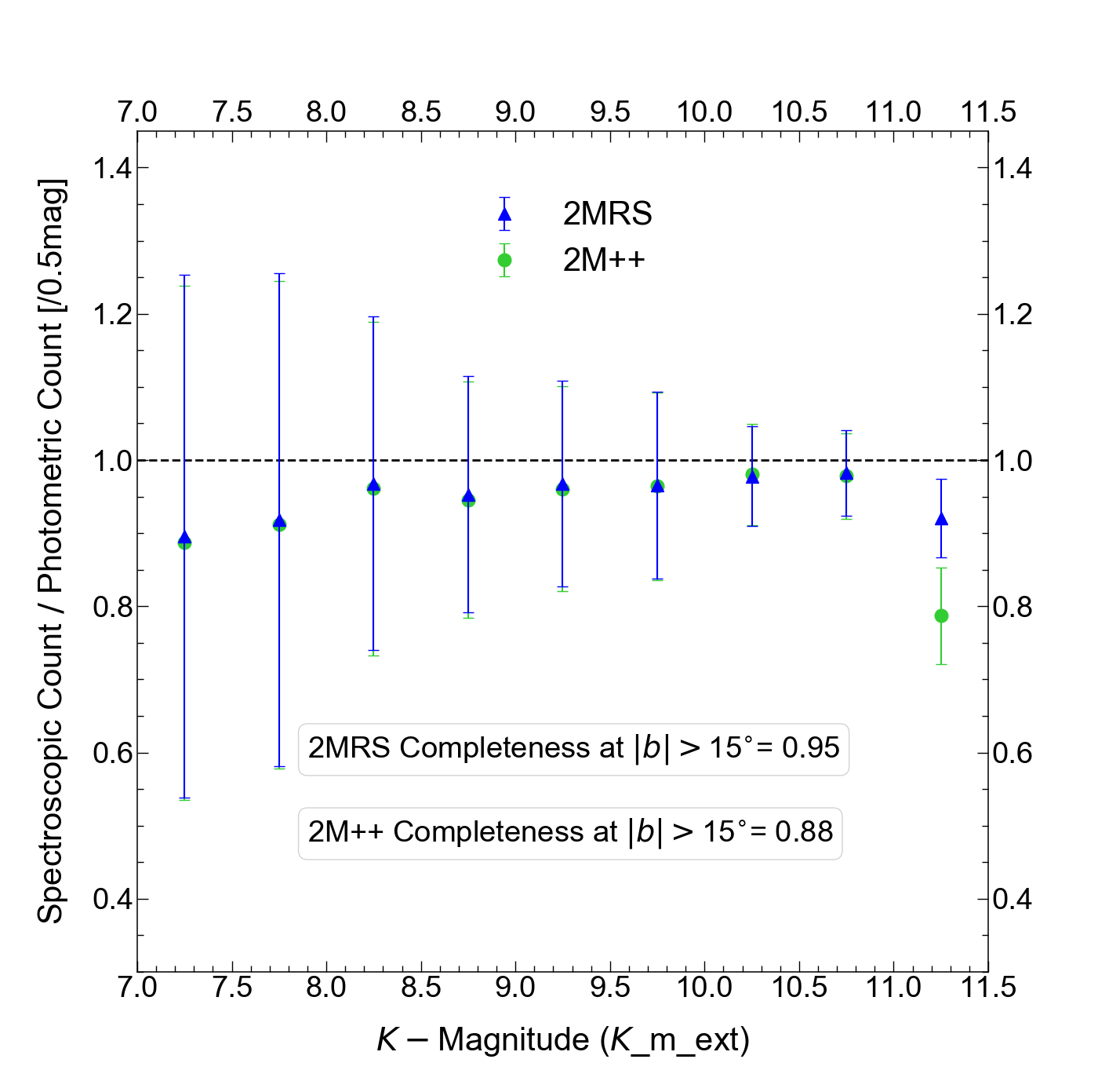
Figure 12: The $K-$band spectroscopic completeness of 2MRS and 2M++ with respect to the 2MASS Extended Source Catalogue, evaluated per half magnitude bin to the limit $K<11.5$. Errors have been calculated using the field-field method.

References

- Abell et al. (1989) Abell G. O., Corwin Harold G. J., Olowin R. P., 1989, ApJS, 70, 1
- Baldry et al. (2010) Baldry I. K., et al., 2010, MNRAS, 404, 86
- Baldry et al. (2018) Baldry I. K., et al., 2018, MNRAS, 474, 3875
- Bilicki et al. (2014) Bilicki M., Jarrett T. H., Peacock J. A., Cluver M. E., Steward L., 2014, ApJS, 210, 9
- Böhringer et al. (2015) Böhringer H., Chon G., Bristow M., Collins C. A., 2015, A&A, 574, A26
- Böhringer et al. (2020) Böhringer H., Chon G., Collins C. A., 2020, A&A, 633, A19
- Boruah et al. (2020) Boruah S. S., Hudson M. J., Lavaux G., 2020, MNRAS, 498, 2703
- Bruzual & Charlot (2003) Bruzual G., Charlot S., 2003, MNRAS, 344, 1000
- Busswell et al. (2004) Busswell G. S., Shanks T., Frith W. J., Outram P. J., Metcalfe N., Fong R., 2004, MNRAS, 354, 991
- Collins et al. (2016) Collins C. A., Böhringer H., Bristow M., Chon G., 2016, in van de Weygaert R., Shandarin S., Saar E., Einasto J., eds, IAU Symposium Vol. 308, The Zeldovich Universe: Genesis and Growth of the Cosmic Web. pp 585–588, doi:10.1017/S1743921316010620
- Driver et al. (2009) Driver S. P., et al., 2009, Astronomy and Geophysics, 50, 5.12
- Driver et al. (2016) Driver S. P., et al., 2016, MNRAS, 455, 3911
- Ebeling et al. (1998) Ebeling H., Edge A. C., Bohringer H., Allen S. W., Crawford C. S., Fabian A. C., Voges W., Huchra J. P., 1998, MNRAS, 301, 881
- Einasto et al. (1997) Einasto M., Tago E., Jaaniste J., Einasto J., Andernach H., 1997, A&AS, 123, 119
- Frith et al. (2003) Frith W. J., Busswell G. S., Fong R., Metcalfe N., Shanks T., 2003, MNRAS, 345, 1049
- Frith et al. (2005a) Frith W. J., Shanks T., Outram P. J., 2005a, MNRAS, 361, 701
- Frith et al. (2005b) Frith W. J., Outram P. J., Shanks T., 2005b, MNRAS, 364, 593
- Frith et al. (2006) Frith W. J., Metcalfe N., Shanks T., 2006, MNRAS, 371, 1601
- Gaia Collaboration et al. (2016) Gaia Collaboration et al., 2016, A&A, 595, A1
- Gaia Collaboration et al. (2018) Gaia Collaboration et al., 2018, A&A, 616, A1
- Gaia Collaboration et al. (2021) Gaia Collaboration et al., 2021, A&A, 649, A1
- Geach et al. (2017) Geach J. E., et al., 2017, ApJS, 231, 7
- Huchra et al. (2012) Huchra J. P., et al., 2012, ApJS, 199, 26
- Jarvis et al. (2013) Jarvis M. J., et al., 2013, MNRAS, 428, 1281
- Jasche & Lavaux (2019) Jasche J., Lavaux G., 2019, A&A, 625, A64
- Keenan et al. (2013) Keenan R. C., Barger A. J., Cowie L. L., 2013, ApJ, 775, 62
- Kenworthy et al. (2019) Kenworthy W. D., Scolnic D., Riess A., 2019, ApJ, 875, 145
- Krolewski et al. (2020) Krolewski A., Ferraro S., Schlafly E. F., White M., 2020, J. Cosmology Astropart. Phys., 2020, 047
- Lavaux & Hudson (2011) Lavaux G., Hudson M. J., 2011, MNRAS, 416, 2840
- Lindegren et al. (2018) Lindegren L., et al., 2018, A&A, 616, A2
- Loveday (2000) Loveday J., 2000, MNRAS, 312, 557
- Mackenzie et al. (2017) Mackenzie R., Shanks T., Bremer M. N., Cai Y.-C., Gunawardhana M. L. P., Kovács A., Norberg P., Szapudi I., 2017, MNRAS, 470, 2328
- Maddox et al. (1990) Maddox S. J., Sutherland W. J., Efstathiou G., Loveday J., Peterson B. A., 1990, MNRAS, 247, 1P
- Maller et al. (2005) Maller A. H., McIntosh D. H., Katz N., Weinberg M. D., 2005, ApJ, 619, 147
- McIntosh et al. (2006) McIntosh D. H., Bell E. F., Weinberg M. D., Katz N., 2006, MNRAS, 373, 1321
- Metcalfe et al. (1991) Metcalfe N., Shanks T., Fong R., Jones L. R., 1991, MNRAS, 249, 498
- Metcalfe et al. (2001) Metcalfe N., Shanks T., Campos A., McCracken H. J., Fong R., 2001, MNRAS, 323, 795
- Metcalfe et al. (2006) Metcalfe N., Shanks T., Weilbacher P. M., McCracken H. J., Fong R., Thompson D., 2006, MNRAS, 370, 1257
- Norberg et al. (2002) Norberg P., et al., 2002, MNRAS, 336, 907
- Planck Collaboration et al. (2018) Planck Collaboration et al., 2018, arXiv e-prints, p. arXiv:1807.06209
- Riess et al. (2016) Riess A. G., et al., 2016, ApJ, 826, 56
- Riess et al. (2018a) Riess A. G., Casertano S., Kenworthy D., Scolnic D., Macri L., 2018a, arXiv e-prints, p. arXiv:1810.03526
- Riess et al. (2018b) Riess A. G., et al., 2018b, ApJ, 861, 126
- Sawala et al. (2022) Sawala T., McAlpine S., Jasche J., Lavaux G., Jenkins A., Johansson P. H., Frenk C. S., 2022, MNRAS, 509, 1432
- Schlafly & Finkbeiner (2011) Schlafly E. F., Finkbeiner D. P., 2011, ApJ, 737, 103
- Secrest et al. (2021) Secrest N. J., von Hausegger S., Rameez M., Mohayaee R., Sarkar S., Colin J., 2021, ApJ, 908, L51
- Sedgwick et al. (2021) Sedgwick T. M., Collins C. A., Baldry I. K., James P. A., 2021, MNRAS, 500, 3728
- Shanks (1990) Shanks T., 1990, in Bowyer S., Leinert C., eds, IAU Symposium Vol. 139, The Galactic and Extragalactic Background Radiation. p. 269
- Shanks et al. (2019a) Shanks T., Hogarth L. M., Metcalfe N., 2019a, MNRAS, 484, L64
- Shanks et al. (2019b) Shanks T., Hogarth L. M., Metcalfe N., Whitbourn J., 2019b, MNRAS, 490, 4715
- Skrutskie et al. (2006) Skrutskie M. F., et al., 2006, AJ, 131, 1163
- Whitbourn & Shanks (2014) Whitbourn J. R., Shanks T., 2014, MNRAS, 437, 2146
- Whitbourn & Shanks (2016) Whitbourn J. R., Shanks T., 2016, MNRAS, 459, 496