On the Transfer of Polarization from the Initial to the Final Proton
in the Elastic Process $e\vec{p}\to e\vec{p}$

Abstract

The $Q^{2}$ dependence of the ratio of the cross sections with and without proton spin flip, as well as the polarization asymmetry in the process $e\vec{p}\to e\vec{p}$ has been numerically analyzed using the results of JLab’s polarization experiments on the measurements of the ratio of the Sachs form factors in the $\vec{e}p\to e\vec{p}$ process. The calculations have been made for the case where the initial (at rest) and final protons are fully polarized and have a common spin quantization axis, which coincides with the direction of motion of the final proton. The longitudinal polarization transfer to the proton has been calculated in the case of the partially polarized initial proton for a kinematics used in the experiment reported in [A. Liyanage et al. (SANE Collaboration), Phys. Rev. C 101, 035206 (2020)], where the double spin asymmetry was measured in the $\vec{e}\vec{p}\to ep$ process. A noticeable sensitivity of the polarization transfer to the proton to the form of the $Q^{2}$ dependence of the ratio $\mu_{p}G_{E}/G_{M}$ has been found. This sensitivity may be used to conduct a new independent experiment to measure this dependence in the $e\vec{p}\to e\vec{p}$ process. A criterion to assess the reliability of measurements of the ratio of Sachs form factors using the Rosenbluth technique has been proposed and used to analyze the results of two experiments.

Introduction. The electric $G_{E}$ and magnetic $G_{M}$ form factors, the so-called Sachs form factors (SFFs), have been experimentally studied since the mid-1950s in the elastic scattering of unpolarized electrons off a proton. All experimental data on the behavior of the SFFs have been obtained by applying the Rosenbluth technique (RT), which is based on using the Rosenbluth cross section (in the one-photon approximation) for the $ep\to ep$ process in the rest frame of the initial proton Rosen :

$$\sigma=\frac{d\sigma}{d\Omega_{e}}=\frac{\alpha^{2}E_{2}\cos^{2}(\theta_{e}/2)}{4E_{1}^{3}\sin^{4}(\theta_{e}/2)}\frac{1}{1+\tau_{p}}\left(G_{E}^{2}+\frac{\tau_{p}}{\varepsilon}G_{M}^{2}\right).$$ (1)

Here, $\tau_{p}=Q^{2}/4M^{2},Q^{2}=-q^{2}=4E_{1}E_{2}\sin^{2}(\theta_{e}/2)$ is the square of the momentum transfer to the proton; $M$ is the mass of the proton; $E_{1}$ and $E_{2}$, are the energies of the initial and final electrons, respectively; $\theta_{e}$ is the electron scattering angle; $\varepsilon=[1+2(1+\tau_{p})\tan^{2}(\theta_{e}/2)]^{-1}$ is the degree of linear polarization of the virtual photon Dombey ; Rekalo74 ; AR ; GL97 that varies in the range $0\leqslant\varepsilon\leqslant 1$; and $\alpha=1/137$ is the fine structure constant.

Formula (1) shows that the main contribution to the cross section for the process $ep\to ep$ at high $Q^{2}$ values comes from the term proportional to $G_{M}^{\,2}$. Because of this, extracting the contribution of $G_{E}^{\,2}$ even at $Q^{2}\geqslant 1$ GeV² becomes a challenging problem ETG15 ; Punjabi2015 . The RT was used to determine the experimental dependence of SFFs on $Q^{2}$, which is described up to $Q^{2}\approx 6$ GeV² by the dipole approximation; their ratio

$$R\equiv\mu_{p}G_{E}/G_{M}$$ (2)

is quite accurately approximated by the equality $R\approx 1$, where $\mu_{p}$=2.79 is the magnetic moment of the proton.

Akhiezer and Rekalo Rekalo74 proposed a method to measure the ratio $R$ that is based on the polarization transfer from the initial electron to the final proton in the process $\vec{e}p\to e\vec{p}$. Precision experiments based on this method conducted at JLab Jones00 ; Gay01 ; Gay02 revealed that the ratio $R$ decreases rapidly with increasing $Q^{2}$, which indicates that the dipole dependence (scaling) of the SFFs is violated. This decrease proved to be linear in the range $0.4\,\mbox{GeV}^{2}\leqslant Q^{2}\,\leqslant 5.6$ GeV².

Measurements of $R$, which were repeated with a higher accuracy Pun05 ; Puckett10 ; Puckett12 ; Puckett17 ; Qattan2005 in a broad $Q^{2}$ range up to 8.5 GeV² using both the Akhiezer – Rekalo method Rekalo74 and the RT, only confirmed these disagreements.

Experimental values of $R$ Liyanage2020 were obtained by the SANE collaboration using the third approach. Namely, they were extracted from the measurements of the double spin asymmetry in the process $\vec{e}\vec{p}\to ep$ in the case where the electron beam and the proton target are partially polarized. The degree of polarization of the proton target was $P_{t}=(70\pm 5)$%. The experiment was carried out at two electron beam energies $E_{1}=5.895$ and 4.725 GeV and two values of $Q^{2}=2.06$ and 5.66 GeV². The values of $R$ obtained in Liyanage2020 are in good agreement with the results of previous polarization experiments carried out in Jones00 ; Gay01 ; Gay02 ; Pun05 ; Puckett10 ; Puckett12 ; Puckett17 .

The fourth method was proposed in JETPL18 . This method allows extracting $G_{E}^{\,2}$ and $G_{M}^{\,2}$ from the direct measurements of cross sections with and without proton spin flip in the elastic process with the polarization transfer from the initial to the final proton:

$$e(p_{1})+\vec{p}\,(q_{1},s_{1})\to e(p_{2})+\vec{p}\,(q_{2},s_{2}),$$ (3)

when the initial (at rest) proton is fully polarized along the direction of motion of the detected final recoil proton. This method, which is also applicable in the two-photon exchange (TPE) approximation, enables measurement of the squares of absolute values of the generalized SFFs in a similar way JETPL19 .

In this study, we use the results of JLab’s polarization experiments, where the ratio $R$ was measured in the process $\vec{e}p\to e\vec{p}$, to numerically analyze the $Q^{2}$ dependence of the ratio of the cross sections with and without proton spin flip and the polarization asymmetry in the process $e\vec{p}\to e\vec{p}$ in the case where the initial (at rest) and final protons are fully polarized and have a common spin quantization axis that coincides with the direction of motion of the detected final recoil proton. In the case of the partially polarized initial proton, the longitudinal polarization transfer to the proton was calculated in the kinematics of the experiment Liyanage2020 . A criterion to assess the reliability of the measured $R$ ratio using the RT is proposed, which is used to analyze the measurements made in two well-known experiments Andivahis1994 ; Qattan2005 .

Cross section for the process $e\vec{p}\to e\vec{p}$ in the rest frame of the initial proton. Let us consider spin 4-vectors $s_{1}$ and $s_{2}$ of the initial and final protons with 4-momenta $q_{1}$ and $q_{2}$, respectively, in process (3) in an arbitrary reference frame. The conditions of orthogonality ($s_{i}q_{i}=0$) and normalization ($s_{i}^{2}=-1$) unambiguously provide the following expressions for the time ($s_{i0}$) and space ($\mbox{\boldmath$s$}_{i}$) components of these spin 4-vectors $s_{i}=(s_{i0},\mbox{\boldmath$s$}_{i})$ in terms of their 4-velocities $v_{i}=q_{i}/M$ ($i=1,2$):

$$s_{i}=(s_{i0},\mbox{\boldmath$s$}_{i}),\;s_{i0}=\mbox{\boldmath$v$}_{i}\,\mbox{\boldmath$c$}_{i},\;\mbox{\boldmath$s$}_{i}=\mbox{\boldmath$c$}_{i}+\frac{(\mbox{\boldmath$c$}_{i}\mbox{\boldmath$v$}_{i})\,\mbox{\boldmath$v$}_{i}}{1+v_{i0}}\;,$$ (4)

where the unit 3-vectors $\mbox{\boldmath$c$}_{i}$ ($\mbox{\boldmath$c$}_{i}^{2}=1$) specify the spin projection (quantization) axes.

In the laboratory reference frame, where $q_{1}=(M,\mbox{\boldmath$0$})$ and $q_{2}=(q_{20},\mbox{\boldmath$q$}_{2})$, the spin projection axes $\mbox{\boldmath$c$}_{1}$ and $\mbox{\boldmath$c$}_{2}$ are chosen such that they coincide with the direction of motion of the final proton:

$$\mbox{\boldmath$c$}=\mbox{\boldmath$c$}_{1}=\mbox{\boldmath$c$}_{2}=\mbox{\boldmath$n$}_{2}=\mbox{\boldmath$q_{2}$}/|\mbox{\boldmath$q$}_{2}|\,.$$ (5)

Then the spin 4-vectors $s_{1}$ and $s_{2}$ of the initial and final protons, respectively, in the laboratory reference frame have the form

$$s_{1}=(0,\mbox{\boldmath$n$}_{2})\,,\;s_{2}=(|\mbox{\boldmath$v$}_{2}|,v_{20}\,\mbox{\boldmath$n_{2}$})\,,\,\mbox{\boldmath$n$}_{2}=\mbox{\boldmath$q_{2}$}/|\mbox{\boldmath$q$}_{2}|\,.$$ (6)

Method JETPL18 is based on the formula for differential cross section for process (3) in the laboratory reference frame in the case where the initial and final protons are polarized and have a common axis of the spin projections $c$ given by Eq. (5):

$$\frac{d\sigma_{\delta_{1},\delta_{2}}}{d\Omega_{e}} = \omega_{+}\sigma^{\uparrow\uparrow}+\omega_{-}\sigma^{\downarrow\uparrow}\,,$$ (7)

$$\sigma^{\uparrow\uparrow} = \sigma_{M}\,G^{2}_{E},\;\;\sigma^{\downarrow\uparrow}=\sigma_{M}\frac{\tau_{p}}{\varepsilon}\,G^{2}_{M}\,,$$ (8)

$$\sigma_{M} = \frac{\alpha^{2}E_{2}\cos^{2}(\theta_{e}/2)}{4E_{1}^{\,3}\sin^{4}(\theta_{e}/2)}\frac{1}{1+\tau_{p}}\,.$$ (9)

Here, $\omega_{\pm}$ are the polarization factors specified by the formulas

$$\omega_{+}=(1+\delta_{1}\delta_{2})/2,\,\,\omega_{-}=(1-\delta_{1}\delta_{2})/2\,,$$ (10)

where $\delta_{1,2}$ are the double projections of the spins of the initial and final protons on the common axis of spin projections $c$ (5). It should be noted that Eq. (7) is valid at $-1\leqslant\delta_{1,2}\leqslant 1$.

The corresponding experiment to measure the squares of the SFFs in the processes with and without proton spin flip can be implemented in the following way. The initial proton at rest should be fully polarized along the direction of motion of the detected final recoil proton. By measuring the differential cross sections $\sigma^{\uparrow\uparrow}$ and $\sigma^{\downarrow\uparrow}$ (8) as functions of $Q^{2}$, it is possible to determine the $Q^{2}$ dependence of $G_{E}^{2}$ and $G^{2}_{M}$ and to measure in this way these form factors.

It is noteworthy that Eq. (7), similar to Eq. (1), is the sum of two terms one of which contains only $G_{E}^{\,2}$ and the second contains only $G_{M}^{\,2}$. By averaging and summing Eq. (7) over the polarizations of the initial and final protons, the Rosenbluth cross section given by Eq. (1) and denoted as $\sigma_{R}$ can be represented in the alternative form JETPL18

$$\sigma_{R}=\sigma^{\uparrow\uparrow}+\sigma^{\downarrow\uparrow}\,.$$ (11)

Consequently, the two terms one of which contains only $G_{E}^{~{}2}$ and the second contains only $G_{M}^{~{}2}$ in the representation of Rosenbluth formula (1) in the form of Eq. (11) physically mean the cross sections with and without proton spin flip, respectively, in the case where the initial proton at rest is fully polarized along the direction of motion of the final proton.

It is often asserted in publications, including textbooks on elementary particle physics, that the SFFs are employed simply because of convenience since they enable the representation of the Rosenbluth formula in a straightforward and concise form. Since such formal conclusions regarding advantages of using the form factors are also contained in popular monographs published many years ago AB ; BLP , they are not subject to criticism and are still reproduced in the literature; see, e.g., Paket2015 .

Cross section (7) can be represented in the form

$$d\sigma_{\delta_{1},\delta_{2}}/d\Omega_{e}=(1+\delta_{2}\delta_{f})(\sigma^{\uparrow\uparrow}+\sigma^{\downarrow\uparrow}),$$ (12)

$$\delta_{f}=\delta_{1}(R_{\sigma}-1)/(R_{\sigma}+1),$$ (13)

$$R_{\sigma}=\sigma^{\uparrow\uparrow}/\sigma^{\downarrow\uparrow},$$ (14)

where $\delta_{f}$ is the degree of the longitudinal polarization of the final proton. If the initial proton is fully polarized ($\delta_{1}=1$), $\delta_{f}$ coincides with the standard definition of polarization asymmetry

$$A=(R_{\sigma}-1)/(R_{\sigma}+1)\;.$$ (15)

As follows from Eq. (8), the ratio of the cross sections with and without proton spin flip $R_{\sigma}$ (14) can be represented in terms of the experimentally measurable quantity $R\equiv\mu_{p}\,G_{E}/G_{M}$:

$$R_{\sigma}=\frac{\sigma^{\uparrow\uparrow}}{\sigma^{\downarrow\uparrow}}=\frac{\varepsilon}{\tau_{p}}\,\frac{G_{E}^{2}}{G_{M}^{2}}=\frac{\varepsilon}{\tau_{p}}\frac{R^{2}}{\mu_{p}^{2}}.$$ (16)

The expression on the right-hand side of Eq. (16) for $R_{\sigma}$ is quite frequently used in publications. For example, the authors of Qattan2015 reported two formulas for the reduced cross sections for the $ep\to ep$ process that include $R_{\sigma}$; however, they seem to be unaware of its physical meaning.

Using the standard notation and replacing $\delta_{f}$ with $P_{r}$ and $\delta_{1}$ with $P_{t}$, we rewrite Eq. (13) for the degree of longitudinal polarization of the final proton in the alternative form

$$P_{r}=P_{t}(R_{\sigma}-1)/(R_{\sigma}+1).$$ (17)

Inverting the connection in (17), we obtain an expression for $R^{2}$ as a function of $P_{r}/P_{t}$:

$$R^{2}=\mu_{p}^{2}\,\frac{\tau_{p}}{\varepsilon}\,\frac{1+R_{p}}{1-R_{p}},\;\;R_{p}=\frac{P_{r}}{P_{t}}\,,$$ (18)

which can be used to extract the ratio $R$ in the proposed method of the polarization transfer from the initial to the final proton.

We calculate the $Q^{2}$ dependence of the polarization asymmetry $A$ (15), the ratio of the cross sections $R_{\sigma}$ (16), and the polarization transfer to the proton $P_{r}$ (17) for both cases where the dipole dependence is valid ($R=R_{d}$) and is violated ($R=R_{j}$):

$$~{}~{}~{}~{}~{}~{}~{}~{}~{}~{}~{}~{}~{}~{}~{}~{}~{}~{}~{}~{}~{}~{}~{}~{}~{}~{}R_{d}=1,$$ (20)

$$R_{j}=\frac{1}{1+0.1430Q^{2}-0.0086Q^{4}+0.0072Q^{6}}.~{}~{}~{}~{}$$

The formula for $R_{j}$ is taken from Qattan2015 ; Kelly’s parametrization Kelly2004 can be used instead.

Numerical results and discussion. To identify general characteristics, Figs. 1 and 2 show the $x=Q^{2}$ dependencies of the ratio of cross sections $R_{\sigma}$ (16) and polarization asymmetry $A$ (15), respectively, calculated numerically with (lines $Rd1,Rd2,\ldots,Rd6$ and $Ad1,Ad2,\ldots,Ad6)$ $R=R_{d}$ given by Eq. (20) and (lines $Rj1,Rj2,\ldots,Rj6$ and $Aj1,Aj2,\ldots,Aj6$) $R=R_{j}$ given by Eq. (20) for the electron-beam energies $E_{1}=1,2,\ldots,6$ GeV, respectively.

The plots displayed in Fig. 1 show that the ratio of the cross sections with and without proton spin flip $R_{\sigma}$ (16) for all electron beam energies decreases with increasing $Q^{2}$. However, this decrease at $R=R_{j}$ is faster than in the case of dipole dependence ($R=R_{d}$) owing to the presence of the denominator in Eq. (20) for $R_{J}$. It should also be noted that the difference in the behavior of the ratio $R_{\sigma}$ (16) calculated with $R=R_{d}$ and $R_{j}$ is insignificant at a low electron-beam energy.

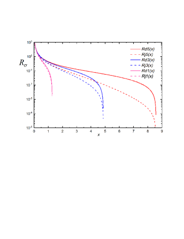
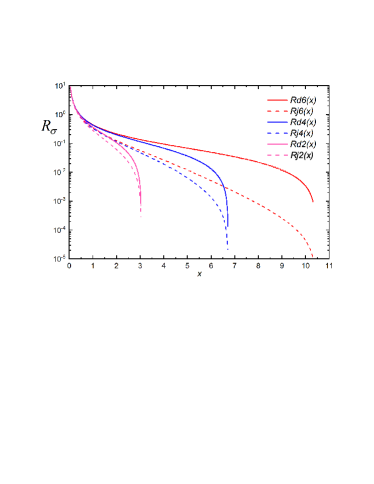
Figure 1: Ratio $R_{\sigma}$ (16) calculated with (lines $Rd1$, $Rd2$,…,$Rd6$) $R=R_{d}$ given by Eq. (20) and (lines $Rj1$, $Rj2$, …,$Rj6$) $R=R_{j}$ given by Eq. (20) versus $Q^{2}$ (GeV²) for the energies $E_{1}=1,2,...,6$ GeV, respectively.

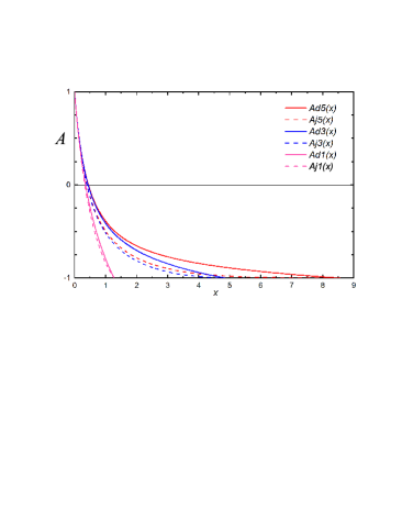
Figure 2: Polarization asymmetry $A$ (15) calculated with (lines $Ad1$, $Ad2$,…,$Ad6$) $R=R_{d}$ given by Eq. (20) and (lines $Aj1$, $Aj2$,…,$Aj6$) $R=R_{j}$ given by Eq. (20) versus $Q^{2}$ (GeV²) for the energies $E_{1}=1,2,...,6$ GeV, respectively.

As seen in Fig. 1, the $Q^{2}$ dependence of $R_{\sigma}$ for each electron-beam energy has a sharp boundary at $Q^{2}_{max}$, which is the maximum possible value of $Q^{2}$ that corresponds to the backscattering of the electron, i.e., scattering at $180^{\circ}$. The values $Q^{2}_{max}$ for each electron-beam energy $E_{1}=1,2,...,6$ GeV are presented in Table 1, which shows that $Q^{2}_{max}$ does not exceed 10.45 GeV² for all energies under consideration.

Table 1: Values of $Q^{2}_{max}$ that set the boundaries of the $Q^{2}$ spectra of $R_{\sigma}$ and the values of $(Q_{0})_{\{d,j\}}^{2}$ at which $\sigma^{\uparrow\uparrow}=\sigma^{\downarrow\uparrow}$; the polarization asymmetry (15) is zero in this case

$E_{1}$ (GeV)	1.0	2.0	3.0	4.0	5.0	6.0
$Q^{2}_{max}$ (GeV2)	1.277	3.040	4.868	6.718	8.578	10.443
$(Q_{0}^{2})_{d}$ (GeV2)	0.358	0.424	0.435	0.446	0.446	0.446
$(Q_{0}^{2})_{j}$ (GeV2)	0.336	0.380	0.391	0.402	0.402	0.402

Table 1 also displays the values of $(Q_{0}^{2})_{\{d,j\}}$ that correspond to the coinciding cross sections with and without proton spin flip; in this case, their ratio is $R_{\sigma}=1$, and the polarization asymmetry is zero. In the case of dipole dependence, $(Q_{0}^{2})_{d}\approx M^{2}/2$, where $M$ is the mass of the proton. If the dipole dependence is violated, $(Q_{0}^{2})_{j}\approx 0.40$ GeV²; i.e., the cross sections $\sigma^{\uparrow\uparrow}$ and $\sigma^{\downarrow\uparrow}$ become equal at approximately the same point where the linear decrease in the ratio $R$ begins. Thus, the points where $Q^{2}=Q_{0}^{2}$ are in a certain sense specific.

If $Q^{2}>Q_{0}^{2}$, the spin-flip cross section $\sigma^{\downarrow\uparrow}$ exceeds the cross section without spin flip $\sigma^{\uparrow\uparrow}$, and their ratio is then $R_{\sigma}<1$. As a result, the helicity carried away by the recoil proton becomes negative. Its absolute value reaches a maximum value of 1 for the backscattered electron.

The calculations represented in Fig. 1 make it possible to understand why measurements of the ratio $R$ using the RT at high $Q^{2}$ values are difficult. They should be conducted in a kinematics where the relative contribution of the $\sigma^{\uparrow\uparrow}$ term to the cross section $\sigma_{R}$ (11) exceeds the accuracy $\Delta_{0}$ with which the Rosenbluth cross section is measured in this experiment:

$$\frac{\sigma^{\uparrow\uparrow}}{\sigma^{\uparrow\uparrow}+\sigma^{\downarrow\uparrow}}=\frac{R_{\sigma}}{(1+R_{\sigma})}>\Delta_{0}.$$ (21)

The restrictions on the kinematics of experiments where the RT is used have not yet been considered in publications, including Egle_2018 ; Gramolin2016 ; Blunden2020 . This problem is nevertheless of importance and deserves special attention.

According to Eq. (21), the kinematics of the conducted experiment should satisfy the condition

$$R_{\sigma}>\Delta_{0},$$ (22)

which can be considered as a necessary condition for reliable measurements and can be used as a criterion for the reliability of measurements.

Table 2: Values of $R_{\sigma}$ (16) calculated with $R=R_{d}$ given by Eq. (20) for the electron-beam energies $E_{1}=1,2,...,6$ GeV and $Q^{2}=1,2,...,9$ GeV²

$Q^{2}$ (GeV2)	1.0	2.0	3.0	4.0	5.0	6.0	7.0	8.0	9.0
$Rd6$, 6 GeV	0.444	0.215	0.136	0.095	0.068	0.049	0.034	0.022	0.012
$Rd5$, 5 GeV	0.440	0.209	0.129	0.086	0.057	0.036	0.020	0.006
$Rd4$, 4 GeV	0.432	0.199	0.115	0.068	0.037	0.013
$Rd3$, 3 GeV	0.415	0.175	0.084	0.031
$Rd2$, 2 GeV	0.365	0.105
$Rd1$, 1 GeV	0.114

Table 3: Values of $R_{\sigma}$ (16) calculated with $R=R_{d}$ given by Eq. (20) for $E_{1}$ and $Q^{2}$ values used in the measurements in Andivahis1994

Q2 (GeV2)	1.75	2.50	3.25	4.00	5.00	6.00	7.00	8.83
$Rd9$, 9.800 GeV				0.107	0.083	0.067	0.055
$Rd8$, 5.507 GeV	0.246	0.165	0.120	0.091	0.064			0.006
$Rd7$, 4.507 GeV				0.079	0.049		0.009
$Rd6$, 3.956 GeV		0.157	0.100	0.067	0.035	0.012
$Rd5$, 3.400 GeV		0.136	0.085	0.049	0.016
$Rd4$, 2.837 GeV		0.114	0.059	0.022
$Rd3$, 2.407 GeV	0.182	0.087	0.029
$Rd2$, 1.968 GeV		0.041
$Rd1$, 1.511 GeV	0.065

Table 2 summarizes the values of $R_{\sigma}$ (16) calculated with $R=R_{d}$ for $E_{1}=1,2,\ldots,6$ GeV and $Q^{2}=1,2,\ldots,9$ GeV² corresponding to the $Rd1,Rd2,...,Rd6$ plots in Fig. 1. All $R_{\sigma}$ values in Table 2 for $Q^{2}=7.0$ and 8.0 GeV², except one where $R_{\sigma}=0.006$, satisfy the inequality $R_{\sigma}\geqslant 0.020$. Using criterion (22), we conclude that the RT-based measurements at $Q^{2}=7.0$ GeV² should be carried out with an accuracy of no less than 1.9 %, while the measurements made at $Q^{2}=8.0$ GeV² require an accuracy of $0.3\div 0.5$ %. Thus, RT measurements of the ratio $R$ at high $Q^{2}$ values is difficult because the relative contribution of the $\sigma^{\uparrow\uparrow}$ term to the Rosenbluth cross section (11) decreases, and the accuracy of measuring this quantity should be correspondingly increased. It is noteworthy that measuring the Rosenbluth cross sections with an accuracy better than 2 % using the RT technique was an unrealistic task in old experiments for many reasons Bernauer2014 .

The criterion (22) for the reliability of data does not specify the meaning of the accuracy $\Delta_{0}$ of the measurement of the Rosenbluth cross sections and specific inaccuracies (statistical, systematic, or normalization) determining this accuracy. Analyzing the reliability of the experiment reported Andivahis1994 using results obtained in Blunden2020 , we show below that $\Delta_{0}$ is determined by the normalization uncertainty. After that, the same approach will be applied to analyze the measurements reported in Qattan2005 .

Analysis of the reliability of two well-known experiments. To analyze the reliability of the ratio $R$ measured in the experiment in Andivahis1994 , we calculate the ratio $R_{\sigma}$ (16) for all electron beam energies $E_{1}$ and squares of the momentum transfer to the proton $Q^{2}$ used in this experiment. The corresponding results are presented in Table 3. Empty cells in Table 3 indicate that no measurements were made at the corresponding $E_{1}$ and $Q^{2}$ values.

The values displayed in bold in Table 3 for $Q^{2}\geqslant 5.0$ GeV² are classified as unreliable results. To be confident in this conclusion, we address study Blunden2020 where experiments Qattan2005 ; Andivahis1994 were reanalyzed taking into account the contribution from the TPE. Figure 15b in Blunden2020 shows that measurements at $Q^{2}<5.0$ GeV² in Andivahis1994 with the added TPE contribution agree well with results from Puckett17 ; however, even the inclusion of the TPE fails to remove disagreements at $Q^{2}=5.0$ GeV². For this reason, the lower value in the column for $Q^{2}=5.0$ GeV² in Table 3 is classified as unreliable, i.e., having insufficient accuracy. Table 3 and criterion (22) show that the accuracy of measurements in Andivahis1994 was about $1.7\div 2.1$ %. The normalization uncertainty in measurements of the Rosenbluth cross section, which at all $Q^{2}$ values in Andivahis1994 was 1.77 % (see Andivahis1994 ; Gramolin2016 ; Bernauer2014 ), falls into the same range. Thus, the accuracy of measurements $\Delta_{0}$ appearing in Eq. (22) should be identified with the normalization uncertainty. Given this accuracy (1.77 %), reliability criterion (22) fails for all values on the diagonal of Table 3 at $Q^{2}\geqslant 5.0$ GeV².

The value in Table 3 for $Q^{2}=8.83$ GeV² and $E_{1}=5.507$ GeV corresponds to $R_{\sigma}=0.006$, a value that requires the accuracy of measurements of $0.3\div 0.5$ %. However, this accuracy was attained in the experiment reported in Bernauer2010-1 and performed only in 2010 and, moreover, in the region $Q^{2}<1$ GeV². It should be noted that the statistical, systematic, and normalization uncertainties of measurements at $Q^{2}=8.83$ GeV² in Andivahis1994 are 3.89, 1.12, and 1.77 %, respectively Gramolin2016 . They significantly exceed the measurement accuracy required at $Q^{2}=8.83$ GeV². In addition, the procedure of RT based measurements was violated at $Q^{2}=8.83$ GeV², since measurements should be performed for each $Q^{2}$ value for at least two or better three energies of the electron beam Bernauer2010 .

The results of the reanalysis of the experiment Qattan2005 with the added TPE contribution were also shown in Fig.15 b in Blunden2020 . They are systematically located above the green stripe in that figure that corresponds to the results of polarization experiments in Puckett17 , which at first glance is an indication that measurements Qattan2005 are unreliable. However, this is not true. To analyze the reliability of the RT-based measurements of the $R$ ratio in the experiment reported in Qattan2005 , the ratio $R_{\sigma}$ (16) was calculated for all energies of the electron beam $E_{1}$ and squares of the momentum transfer to the proton $Q^{2}$ used in the experiment. The corresponding results are presented in Table 4.

Table 4: Values of $R_{\sigma}$ (16) calculated with $R=R_{d}$ given by Eq. (20) for $E_{1}$ and $Q^{2}$ values used in the measurements in Qattan2005

$Q^{2}$ (GeV2)	2.64	3.20	4.10
$Rd5$, $E_{1}=4.702$ GeV	0.148	0.115	0.078
$Rd4$, $E_{1}=3.772$ GeV	0.134	0.098	0.058
$Rd3$, $E_{1}=2.842$ GeV	0.102	0.063	0.018
$Rd2$, $E_{1}=2.262$ GeV	0.061	0.018
$Rd1$, $E_{1}=1.912$ GeV	0.020

The accuracy of measurements required for the values given in bold in Table 4 proves to correspond to the normalization accuracy in Qattan2005 equal to 1.7 % Bernauer2014 , thus indicating their reliability. This conclusion is based on the necessity of using the same approach to analyze measurements in Qattan2005 and Andivahis1994 , where $\Delta_{0}$ is determined by the normalization uncertainty. Since measurements in Qattan2005 are reliable, a more accurate reanalysis is required to remove the remaining disagreements between “Qattan2005 + TPE” and Puckett17 discovered in Blunden2020 .

On the feasibility of the measurement of the ratio of SFFs in the $e\vec{p}\to e\vec{p}$ process. The method to measure squares of SFFs in the processes with and without proton spin flip proposed in JETPL18 requires a fully polarized proton target, which may be obtained in the distant future. As stated above, it may be considered in a broader sense as a technique based on the polarization transfer from the initial to the final proton. Generally, if the initial proton is partially polarized, the degree of the longitudinal polarization transfer to the recoil proton is given by Eq. (17). An experiment to measure this quantity is currently quite realistic, since a partially polarized proton target with a high degree of polarization $P_{t}=(70\pm 5)$ % was already used in Liyanage2020 . For this reason, it would be the most expedient to carry out the proposed experiment at the facility used by the SANE collaboration Liyanage2020 at the same value of $P_{t}=0.70$, electron beam energies $E_{1}=4.725$ and 5.895 GeV, and the same values of the square of the momentum transfer to the proton $Q^{2}=2.06$ and 5.66 GeV². The difference between the proposed experiment and that performed in Liyanage2020 is that the electron beam should be unpolarized, while the detected recoil proton should move exactly along the direction of quantization of the proton target spin. The degrees of the longitudinal and transverse polarizations of the final proton were measured in Jones00 ; Gay01 ; Gay02 ; Pun05 ; Puckett10 ; Puckett12 ; Puckett17 . In the proposed experiment, the degree of the longitudinal polarization of the recoil proton alone should be measured, which is an advantage compared to the technique proposed in Rekalo74 .

The calculated $Q^{2}$ dependence of the polarization transfer to the final proton $P_{r}$ (17) in the kinematics of the experiment reported Liyanage2020 is plotted in Fig. 3, where the lines $Pd5$ ($Pd4$) and $Pj5$ ($Pj4$) are obtained with $R=R_{d}$ given by Eq. (20) and with $R=R_{j}$ given by Eq. (20) for the electron beam energy $E_{1}=5.895$ (4.725) GeV, respectively. For all lines in Fig. 3, the degree of polarization of the proton target is $P_{t}=0.70$.

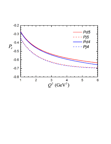
Figure 3: Longitudinal polarization of the recoil proton $P_{r}$ (17) calculated with (lines $Pd5$ and $Pd4$) $R=R_{d}$ given by Eq. (20) and (lines $Pj5$ and $Pj4$) $R=R_{j}$ given by Eq. (20) versus the square of the momentum transfer to the proton $Q^{2}$ (GeV²) for the values $E_{1}$ and $P_{t}$ used in Liyanage2020 .

The plots in Fig. 3 show that the polarization transfer to the final proton significantly depends on the form of the $Q^{2}$ dependence of $R$. The absolute value of this polarization transfer in the case of the violation of the SFFs scaling, i.e., in the case $R=R_{j}$, is significantly greater than that in the case $R=R_{d}$. A quantitative estimate of this difference is shown in Table 5, where the longitudinal polarizations of the recoil proton $Pj5$, $Pd5$, $Pj4$, and $Pd4$, as well as their relative differences $\Delta_{dj5}=(Pj5-Pd5)/Pj5$ and $\Delta_{dj4}=(Pj4-Pd4)/Pj4$ in percent, are displayed for two electron-beam energies of 5.895 and 4.725 GeV and two values $Q^{2}=2.06$ and 5.66 GeV².

Table 5: Longitudinal polarization of the recoil proton $P_{r}$ (17) for electron-beam energies of 5.895 and 4.725 GeV and $Q^{2}=2.06$ and 5.66 GeV²

$Q^{2}$ (GeV2)	$Pd5$	$Pj5$	$Pd4$	$Pj4$	$\Delta_{dj5}$, %	$\Delta_{dj4}$, %
2.06	–0.46	–0.55	–0.47	–0.56	16.6	16.1
5.66	–0.63	–0.69	–0.65	–0.69	9.1	6.4

Table 5 shows that the relative differences between $Pj5$ and $Pd5$ and between $Pj4$ and $Pd4$ at $Q^{2}=2.06$ GeV² are 16.6 and 16.1 %, respectively, and decrease to 9.1 and 6.4 %, respectively, at $Q^{2}=5.66$ GeV².

Conclusions. Using the results of the JLab’s polarization experiments, where the ratio $R$ was measured in the $\vec{e}p\to e\vec{p}$ process, we have numerically analyzed the ratio of cross sections with and without proton spin flip and the polarization asymmetry as functions of the square of the momentum transfer to the proton in this process for the case where the initial (at rest) proton and the final proton are fully polarized and have a common spin quantization axis that coincides with the direction of motion of the detected recoil proton. If the initial proton is partially polarized, the longitudinal polarization transfer to the proton is calculated for the kinematics used by the SANE collaboration Liyanage2020 in the experiments to measure double spin asymmetry in the $\vec{e}\vec{p}\to ep$ process. A noticeable sensitivity of the polarization transfer to the proton to the form of the $Q^{2}$ dependence of the ratio $R$ has been found. This sensitivity may be used to conduct a new independent experiment to measure this dependence in the $e\vec{p}\to e\vec{p}$ process. A criterion for the reliability of measurements of $R$ using the Rosenbluth technique has been proposed and used to analyze results of two experiments reported in Andivahis1994 ; Qattan2005 . The results of the analysis may be used to identify the reasons for the disagreements that remain between the results of measurements Qattan2005 with the added TPE contribution and polarization experiments Puckett17 , which were discovered in Blunden2020 .

Acknowledgments. I am grateful to R. Lednicky for his interest in the study and helpful discussions.

References

- (1) M. N. Rosenbluth, Phys. Rev. 79, 615 (1950).
- (2) N. Dombey, Rev. Mod. Phys. 41, 236 (1969).
- (3) A. I. Akhiezer and M. P. Rekalo, Sov. J. Part. Nucl. 4, 277 (1974).
- (4) A. I. Akhiezer and M. P. Rekalo, Electrodynamics of Hadrons (Naukova Dumka, Kiev, 1977) [in Russian].
- (5) M. V. Galynskii and M. I. Levchuk, Phys. At. Nucl. 60, 1855 (1997).
- (6) S. Pacetti, R. Baldini Ferroli, and E. Tomasi-Gustafsson, Phys. Rept. 550-551, 1 (2015).
- (7) V. Punjabi, C.F. Perdrisat, M.K. Jones, E.J. Brash, and C.E. Carlson, Eur. Phys. J. A 51, 79 (2015).
- (8) M.K. Jones, K.A. Aniol, F.T. Baker, et al. (JLab Hall A Collab.), Phys. Rev. Lett. 84, 1398 (2000).
- (9) O. Gayou, K. Wijesooriya, A. Afanasev, et al. (JLab Hall A Collab.), Phys. Rev. C 64, 038202 (2001).
- (10) O. Gayou, E.J. Brash, M.K. Jones, et al. (JLab Hall A Collab.), Phys. Rev. Lett. 88, 092301 (2002).
- (11) V. Punjabi, C.F. Perdrisat, K.A. Aniol, et al. (JLab Hall A Collab.), Phys. Rev. C 71, 055202 (2005).
- (12) A. Puckett, J. Brash, O. Gayou, et al. (JLab Hall A Collab.), Phys. Rev. Lett. 104, 242301 (2010).
- (13) A. J. R. Puckett, E. J. Brash, O. Gayou, et al. (JLab Hall A Collab.), Phys. Rev. C 85, 045203 (2012).
- (14) A. J. R. Puckett, E. J. Brash, M. K. Jones, et al., Phys. Rev. C 96, 055203 (2017).
- (15) I. A. Qattan, J. Arrington, R. E. Segel, et al., Phys. Rev. Lett. 94, 142301 (2005).
- (16) A. Liyanage, W. Armstrong, H. Kang, et al. (SANE Collab.), Phys. Rev. C 101, 035206 (2020).
- (17) M.V. Galynskii, JETP Lett. 109, 1 (2019).
- (18) M.V. Galynskii and R.E. Gerasimov, JETP Lett. 110, 646 (2019).
- (19) L. Andivahis, P.E. Bosted, A. Lung, et al., Phys. Rev. D. 50, 5491 (1994).
- (20) A. I. Akhiezer and V. B. Berestetskii, Quantum Electrodynamics (Nauka, Moscow, 1969; Wiley, New York, 1965)
- (21) V. B. Berestetskii, E. M. Lifshitz, and L. P. Pitaevskii, Course of Theoretical Physics, Vol. 4: Quantum Electrodynamics (Nauka, Moscow, 1989; Pergamon, Oxford, 1982).
- (22) A. J. R. Puckett, arXiv: 1508.01456 [nucl-ex].
- (23) I. A. Qattan, J. Arrington, and A. Alsaad, Phys. Rev. C 91, 065203 (2015).
- (24) J. J. Kelly, Phys. Rev. C 70, 068202 (2004).
- (25) E. Tomasi-Gustafsson and S. Pacetti, Few-Body Systems 59, 91 (2018).
- (26) A. V. Gramolin and D. M. Nikolenko, Phys. Rev. C 93, 055201 (2016).
- (27) J. Ahmed, P. G. Blunden, W. Melnitchouk, Phys. Rev. C 102, 045205 (2020).
- (28) J. C. Bernauer, M. O. Distler, J. Friedrich, et al. (A1 Collab.), Phys. Rev. C. 90, 015206 (2014).
- (29) J. C. Bernauer, P. Achenbach, C. Ayerbe Gayoso, et al. (A1 Collab.), Phys. Rev. Lett. 105, 242001 (2010).
-
(30)
J. C. Bernauer, http://inspirehep.net/record/1358265/
files/bernauer.pdf.