A New Representation of Successor Features for Transfer across Dissimilar Environments

Majid Abdolshah    Hung Le    Thommen Karimpanal George    Sunil Gupta    Santu Rana    Svetha Venkatesh
Abstract

Transfer in reinforcement learning is usually achieved through generalisation across tasks. Whilst many studies have investigated transferring knowledge when the reward function changes, they have assumed that the dynamics of the environments remain consistent. Many real-world RL problems require transfer among environments with different dynamics. To address this problem, we propose an approach based on successor features in which we model successor feature functions with Gaussian Processes permitting the source successor features to be treated as noisy measurements of the target successor feature function. Our theoretical analysis proves the convergence of this approach as well as the bounded error on modelling successor feature functions with Gaussian Processes in environments with both different dynamics and rewards. We demonstrate our method on benchmark datasets and show that it outperforms current baselines.

Machine Learning, ICML

1 Introduction

Reinforcement learning (RL) is a computational approach that learns how to attain a complex goal by maximising rewards over time. Successful applications range from Atari games (Mnih et al., 2015), to robotics (Zhang et al., 2017), and self-driving cars (Liang et al., 2018). However, this success is based on solving each task from scratch, and thus training these agents requires vast amounts of data.

Several solutions have been proposed to address this problem. Most works in transfer RL such as Progressive Neural Networks (Rusu et al., 2016) and Inter-Task Mapping setups (Ammar & Taylor, 2011; Gupta et al., 2017; Konidaris & Barto, 2006; Yin & Pan, 2017) assume that the state-action space, or reward distribution space can be disentangled into independent sub-domains. However, learning interpretable, disentangled representations is challenging (Zhu et al., 2020). The dynamics and the reward was decoupled for the first time in  (Barreto et al., 2017). Building upon an elegant formulation called the successor function (Dayan, 1993), the method allowed flexible transfer learning across tasks that differ in their reward structure. The underlying assumption was that the environmental dynamics remains unchanged and using a Generalised Policy Improvement (GPI) method, the optimal policy is determined. Such successor feature based methods have been shown to efficiently transfer knowledge across RL tasks (Barreto et al., 2018, 2019, 2020). Other works that have built upon successor features include generalised policy updates on successor features (Barreto et al., 2020), a universal type of successor feature based on the temporal difference method (Ma et al., 2020), and Variational Universal Successor Features (Siriwardhana et al., 2019) that perform target driven navigation. Option Keyboard (Barreto et al., 2019) leveraged successor features to combine skills to define and manipulate options. This allows for change in reward, but a slight change of the environment can deteriorate the performance of a new task. If however both the environmental dynamics and the reward differs across tasks, these methods are unable to handle this challenge.

In real-world problems when environment dynamics and rewards change across tasks, both these aspects need careful modelling. Failing to do so can lead to negative transfer of knowledge from the previously seen tasks. Thus RL methods using successor features need to be extended to handle the changes in environmental dynamics. Such work is limited. Zhang et al. (Zhang et al., 2017) aim to address this problem by considering a linear relationship between the source and target successor features. This modelling is restrictive and may fall short in capturing the complexity of the changed environment dynamics. Thus, the problem of designing a method using a successor feature based approach to transfer knowledge from source to target environment where the dynamics are dissimilar, is still open.

Our new approach enables the efficient learning of novel successor features to cater to the new target environmental dynamics. This is done by using the distribution of the previous (source) task successor features as a prior for the new target task. We model both the target and source distributions through Gaussian Processes (GPs). The target distribution is modeled as a noisy version of the source distribution. This approach assumes that the source and target environments lie within some proximity to each other i.e. they are similar within some noisy envelope. However, this adjustable noisy envelope impacts the upper bounded error on the modelling of optimal policy in the target environment. The advantage of this approach is that the source observations provide a head-start for the learning process and additional explorations in the target will provide efficient convergence to the optimal policy. We use a GPI method to estimate the target action value function. We provide theoretical analysis and upper bounds (1) on the difference of action-value functions when the optimal policy derived from environment i𝑖i is replaced by the optimal policy derived from environment j𝑗j; (2) on the estimation error of the action-value function of an optimal policy learned in a source environment when executed in the target environment; (3) on the difference of the optimal action-value function in the target environment and our GPI-derived action value function. We evaluate this approach in a variety of benchmark environments with different levels of complexity. Our key contributions are:

  • A new method based on successor features and Gaussian Processes that enhances transfer from source to target tasks when the dynamics of the environment are dissimilar;

  • A theoretical analysis for the new successor based method; and,

  • An empirical comparison on diverse suit of RL benchmarks with different levels of complexity.

2 Background

2.1 Reinforcement Learning

We model the RL framework as a Markov Decision Process (MDP) described as <𝒮,𝒜,p,R><\mathcal{S},\mathcal{A},p,R>, where 𝒮𝒮\mathcal{S} is a finite state space, 𝒜𝒜\mathcal{A} represents a finite action space, p:𝒮×𝒮×𝒜[0,1]:𝑝𝒮𝒮𝒜01p:\mathcal{S}\times\mathcal{S}\times\mathcal{A}\rightarrow[0,1] the transition probabilities, and R:𝒮×𝒜:𝑅𝒮𝒜R:\mathcal{S}\times\mathcal{A}\rightarrow\mathbb{R} is a bounded reward function. A discount factor γ(0,1]𝛾01\gamma\in(0,1] encodes the importance of future rewards with respect to the current state. The objective of RL is to find an optimal policy π(a|s):𝒮𝒜:𝜋conditional𝑎𝑠𝒮𝒜\pi(a|s):\mathcal{S}\rightarrow\mathcal{A} that maps the states to the actions such that it maximises the expected discounted reward. The action-value of policy π𝜋\pi is defined as Qπ(st,at)=𝔼π[k=0γkR(st+k,at+k)|s0=st,a0=at]superscript𝑄𝜋subscript𝑠𝑡subscript𝑎𝑡superscript𝔼𝜋delimited-[]formulae-sequenceconditionalsuperscriptsubscript𝑘0superscript𝛾𝑘𝑅subscript𝑠𝑡𝑘subscript𝑎𝑡𝑘subscript𝑠0subscript𝑠𝑡subscript𝑎0subscript𝑎𝑡Q^{\pi}(s_{t},a_{t})=\mathbb{E}^{\pi}[\sum_{k=0}^{\infty}\ \gamma^{k}R(s_{t+k},a_{t+k})|s_{0}=s_{t},a_{0}=a_{t}], where stsubscript𝑠𝑡s_{t} and atsubscript𝑎𝑡a_{t} are the state of the agent at time step t𝑡t, and the action that is taken in that state, respectively.

Q-Learning: Q-Learning is an off-policy RL approach that aims to learn the optimal action-value function. This function can be updated recursively as:

Qπ(st,at)=𝔼st+1[R(st,at)+γmaxa𝒜(Qπ(st+1,a))].superscript𝑄𝜋subscript𝑠𝑡subscript𝑎𝑡subscript𝔼subscript𝑠𝑡1delimited-[]𝑅subscript𝑠𝑡subscript𝑎𝑡𝛾𝑎𝒜superscript𝑄𝜋subscript𝑠𝑡1𝑎Q^{\pi}(s_{t},a_{t})=\mathbb{E}_{s_{t+1}}\big{[}R(s_{t},a_{t})+\gamma\underset{a\in\mathcal{A}}{\max}\big{(}Q^{\pi}(s_{t+1},a)\big{)}\big{]}. (1)

After learning the action-value function, the optimal policy can be retrieved by selecting the best action at every state: π(s)argmaxa𝒜Q(s,a)superscript𝜋𝑠𝑎𝒜argmaxsuperscript𝑄𝑠𝑎\pi^{*}(s)\in\underset{a\in\mathcal{A}}{\operatorname*{argmax}}\ Q^{*}(s,a). In the next section we draw the connection between Q-Learning and successor features.

2.2 Successor Features

The successor feature representation allows decoupling of the dynamics of an MDP from its reward distributions. Baretto et al. (Barreto et al., 2017) generalised the successor representations that was first formulated in Dayan et al. (Dayan, 1993) decomposing the action-value function into a set of features that encode the dynamics of the environment and a weight that acts as a task-specific reward mapper. This decomposition can be formulated as:

R(s,a)=ϕ(s,a)T𝐰,𝑅𝑠𝑎superscriptbold-italic-ϕabsentsuperscript𝑠𝑎T𝐰R(s,a)={\bm{\phi}}^{\mathrm{}}(s,a)^{\mathrm{T}}{\bf w}, (2)

where ϕ(s,a)Dbold-italic-ϕ𝑠𝑎superscript𝐷{\bm{\phi}}(s,a)\in\mathbb{R}^{D} are the features of (s,a)𝑠𝑎(s,a) that represent the dynamics of the environment and 𝐰𝐰{\bf w} is the reward mapper of the environment. The two components can be learnt through supervised learning (Zhu et al., 2020). Note that ϕ(.,.)\bm{\phi}(.,.) can be any complex model such as a neural network. Baretto et al. (Barreto et al., 2017) showed that this decomposition can be used in the construction of the action-value function. Let us assume a reward function as in Eq. (2), the action value function can be derived as:

Qπ(s,a)superscript𝑄𝜋𝑠𝑎\displaystyle Q^{\pi}(s,a) =𝔼π[R(st+1,at+1)+γR(st+2,at+2)+\displaystyle=\mathbb{E}^{\pi}\big{[}R(s_{t+1},a_{t+1})+\gamma R(s_{t+2},a_{t+2})+
\displaystyle\ldots |st=s,at=a]=𝔼π[t=0γtϕ(st+1,at+1)\displaystyle|s_{t}=s,a_{t}=a\big{]}=\mathbb{E}^{\pi}\big{[}\sum_{t=0}^{\infty}\gamma^{t}\phi(s_{t+1},a_{t+1})
|st=s,at=a]𝐰=𝝍(s,a)T𝐰,\displaystyle|s_{t}=s,a_{t}=a\big{]}{\bf w}={\bm{\psi}}^{\mathrm{}}(s,a)^{\mathrm{T}}{\bf w}, (3)

where 𝝍(s,a)Tsuperscript𝝍absentsuperscript𝑠𝑎T{\bm{\psi}}^{\mathrm{}}(s,a)^{\mathrm{T}} is the “Successor Feature (SF)” of (s,a)𝑠𝑎(s,a) and summarises the dynamics induced by π𝜋\pi. Eq. (3) satisfies the Bellman Equation and and can be learnt through any conventional method. By treating the latent representation ϕ(.,.)\bm{\phi}(.,.) as the immediate reward in the context of Q-Learning, the successor feature function can be written as:

𝝍π(s,a)=ϕ(st,at)+γ𝔼π[𝝍π(st+1,π(st+1))\displaystyle{\bm{\psi}}^{\pi}(s,a)={\bm{\phi}}(s_{t},a_{t})+\gamma\mathbb{E}^{\pi}\big{[}{\bm{\psi}}^{\pi}(s_{t+1},\pi\big{(}s_{t+1})\big{)} |st=s,\displaystyle|s_{t}=s,
at=a].\displaystyle a_{t}=a\big{]}. (4)
Refer to caption
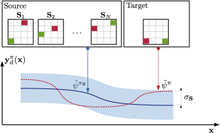
Figure 1: Our proposed approach uses GPs to model the source successor features functions (𝝍~π𝐬superscriptbold-~𝝍subscript𝜋𝐬\bm{\tilde{\psi}}^{\pi_{{\bf s}}}) as noisy measurements for the target successor features functions (𝝍~πsuperscriptbold-~𝝍𝜋\bm{\tilde{\psi}}^{\pi}).

The principal advantage of SFs is that when the knowledge of 𝝍π(s,a)superscript𝝍𝜋𝑠𝑎{\bm{\psi}}^{\pi}(s,a) is observed, one can compute a task-specific reward mapper based on the observations seen in the same environment with different reward function. Given 𝝍π(s,a)superscript𝝍𝜋𝑠𝑎{\bm{\psi}}^{\pi}(s,a), the updated reward mapper 𝐰~~𝐰\tilde{\bm{\mathrm{w}}} for a new reward function can be approximated by solving a regression problem in tabular scenarios (Barreto et al., 2020). This enables us to construct the new action-value function Q~π(s,a)=𝝍π(s,a)T𝐰~superscript~𝑄𝜋𝑠𝑎superscript𝝍𝜋superscript𝑠𝑎Tbold-~𝐰\tilde{Q}^{\pi}(s,a)={\bm{\psi}}^{\pi}(s,a)^{\mathrm{T}}\bm{\tilde{\mathrm{w}}} by only observing few steps of the new reward function in a similar environment. In non-tabular problems, a deep neural network can be used to learn the successor feature functions of an environment by minimising the following loss:

Lψ(𝜽)=||ϕ~(st,at)+\displaystyle L_{\psi}(\bm{\theta})=||{\bf\tilde{\bm{\phi}}}(s_{t},a_{t})+ γt𝝍~π(st+1,at+1;𝜽ψ)superscript𝛾𝑡superscriptbold-~𝝍𝜋subscript𝑠𝑡1subscript𝑎𝑡1subscript𝜽𝜓\displaystyle\gamma^{t}\bm{\tilde{\psi}}^{\pi}(s_{t+1},a_{t+1};\bm{\theta}_{\psi})
𝝍~π(st,at;𝜽ψ)||.\displaystyle-{\bf\tilde{\bm{\psi}}}^{\pi}(s_{t},a_{t};\bm{\theta}_{\psi})||. (5)

Similarly, by having the ϕ(.,.){\bm{\phi}}(.,.) function, the new task-specific reward mapper 𝐰~~𝐰\tilde{\bm{\mathrm{w}}} is computed as:

w(𝐰~)=𝔼(s,a)newtask[(r(s,a)ϕ(s,a)T𝐰~)2].subscript𝑤bold-~𝐰subscript𝔼for-all𝑠𝑎newtaskdelimited-[]superscript𝑟𝑠𝑎superscriptbold-italic-ϕabsentsuperscript𝑠𝑎Tbold-~𝐰2\mathcal{L}_{w}(\bm{\mathrm{\tilde{w}}})=\mathbb{E}_{\forall(s,a)\in\mathrm{new\ task}}\Big{[}\big{(}r(s,a)-{\bm{\phi}^{\mathrm{}}}(s,a)^{\mathrm{T}}\bm{\mathrm{\tilde{w}}}\big{)}^{2}\Big{]}. (6)

where r(s,a)𝑟𝑠𝑎r(s,a) is the obtained reward.

3 Method

We now consider source and target environments with both dissimilar dynamics and different reward functions. The goal of transfer in RL in such problems is to learn an optimal policy for the target environment, by leveraging exterior source information and interior target information (Joy et al., 2019; Shilton et al., 2017). We first define the set of source environments as:

𝐒={(𝒮,𝒜,p1,R1),,(𝒮,𝒜,pN,RN)},superscript𝐒𝒮𝒜subscript𝑝1subscript𝑅1𝒮𝒜subscript𝑝𝑁subscript𝑅𝑁\mathcal{{\mathcal{M^{\mathrm{\mathbf{S}}}}}}=\Big{\{}\mathcal{M}(\mathcal{S},\mathcal{A},p_{1},R_{1}),\ldots,\mathcal{M}(\mathcal{S},\mathcal{A},p_{N},R_{N})\Big{\}},

where (.)\mathcal{M}(.) represents an MDP induced by ϕ(.,.)\mathbf{\bm{\phi}}(.,.) as a feature function used in all environments. We denote the N𝑁N source environments by 𝐒1,,𝐒Nsubscript𝐒1subscript𝐒𝑁{\bf S}_{1},\ldots,{\bf S}_{N} and train an optimal policy in each environment to create a set of policies: Π𝐒={π𝐒1,,π𝐒N}superscriptΠ𝐒superscript𝜋subscript𝐒1superscript𝜋subscript𝐒𝑁\Pi^{\mathrm{\mathbf{S}}}=\big{\{}\pi^{\mathrm{\mathbf{S}}_{1}},\ldots,\pi^{\mathrm{\mathbf{S}}_{N}}\big{\}}. By executing these N𝑁N optimal policies in their corresponding source environments, N𝑁N distinct successor feature functions 𝝍πi,i={1,,N}superscript𝝍subscript𝜋𝑖𝑖1𝑁{\bf\bm{\psi}}^{\pi_{i}},\ i=\{1,\ldots,N\} are computed using the loss function Eq. (5). We define 𝝍πi=𝝍1πi,,𝝍Dπisuperscript𝝍subscript𝜋𝑖superscriptsubscript𝝍1subscript𝜋𝑖superscriptsubscript𝝍𝐷subscript𝜋𝑖{\bf\bm{\psi}}^{\pi_{i}}={\bf\bm{\psi}}_{1}^{\pi_{i}},\ldots,{\bf\bm{\psi}}_{D}^{\pi_{i}} and 𝝍dπisuperscriptsubscript𝝍𝑑subscript𝜋𝑖{\bf\bm{\psi}}_{d}^{\pi_{i}} is the d𝑑d-th dimension. Source successor feature functions can be learnt using neural networks with parameters 𝜽ψsubscript𝜽𝜓\bm{\theta}_{\psi} that can be updated by gradient descent. Algorithm 1 shows how the successor feature functions are computed.

Using state-action pairs as observations, we construct a set of successor feature function samples as: 𝒟𝐒i={(𝐱1𝐒i,𝝍~πi(𝐱1𝐒𝐢)),(𝐱2𝐒i,𝝍~πi(𝐱2𝐒i)),,(𝐱n𝐒i,𝝍~πi(𝐱n𝐒i))},superscript𝒟subscript𝐒𝑖superscriptsubscript𝐱1subscript𝐒𝑖superscriptbold-~𝝍subscript𝜋𝑖superscriptsubscript𝐱1subscript𝐒𝐢superscriptsubscript𝐱2subscript𝐒isuperscriptbold-~𝝍subscript𝜋𝑖superscriptsubscript𝐱2subscript𝐒isuperscriptsubscript𝐱𝑛subscript𝐒isuperscript~𝝍subscript𝜋𝑖superscriptsubscript𝐱𝑛subscript𝐒i\mathcal{D}^{\mathcal{\mathbf{S}}_{i}}=\Big{\{}\big{(}{\bf x}_{1}^{\mathrm{\mathbf{S}}_{i}},{\bf\bm{\tilde{\psi}}}^{\pi_{i}}({\bf x}_{1}^{\mathrm{\mathbf{\mathrm{\mathbf{S}}_{i}}}})\big{)},\big{(}{\bf x}_{2}^{\mathrm{\mathrm{\mathbf{S}}_{i}}},{\bf\bm{\tilde{\psi}}}^{\pi_{i}}({\bf x}_{2}^{\mathrm{{\bf S}_{i}}})\big{)},\ldots,\big{(}{\bf x}_{n}^{\mathrm{\mathrm{\mathbf{S}}_{i}}},{\bf\tilde{\bm{\psi}}}^{\pi_{i}}({\bf x}_{n}^{\mathrm{{\bf S}_{i}}})\big{)}\Big{\}}, where 𝐱t𝐒i=(st,at)superscriptsubscript𝐱𝑡subscript𝐒𝑖subscript𝑠𝑡subscript𝑎𝑡{\bf x}_{t}^{\mathrm{\mathbf{S}}_{i}}=(s_{t},a_{t}) is a tuple of state-action in 𝐒isubscript𝐒𝑖{\bf S}_{i} at time t𝑡t following policy πisubscript𝜋𝑖\pi_{i} and 𝝍~πi(𝐱t𝐒i)superscriptbold-~𝝍subscript𝜋𝑖superscriptsubscript𝐱𝑡subscript𝐒𝑖\bm{\tilde{\psi}}^{\pi_{i}}({\bf x}_{t}^{\mathrm{\mathbf{S}}_{i}})\ is the successor feature for 𝐱t𝐒isuperscriptsubscript𝐱𝑡subscript𝐒𝑖{\bf x}_{t}^{\mathrm{\mathbf{S}}_{i}}. If observations from target environment exist, a set of successor feature function samples in the target environment can be constructed as 𝒟𝓣={(𝐱1𝓣,𝝍~π(𝐱1𝓣)),(𝐱2𝓣,𝝍~π(𝐱2𝓣)),,(𝐱m𝓣,𝝍~π(𝐱m𝓣))},superscript𝒟𝓣superscriptsubscript𝐱1𝓣superscriptbold-~𝝍𝜋superscriptsubscript𝐱1𝓣superscriptsubscript𝐱2𝓣superscript~𝝍𝜋superscriptsubscript𝐱2𝓣superscriptsubscript𝐱𝑚𝓣superscriptbold-~𝝍𝜋superscriptsubscript𝐱𝑚𝓣\mathcal{D}^{\mathcal{\bm{T}}}=\Big{\{}\big{(}{\bf x}_{1}^{\mathcal{\bm{T}}},{\bf\bm{\tilde{\psi}}^{\pi}}({\bf x}_{1}^{\mathcal{\bm{T}}})\big{)},\big{(}{\bf x}_{2}^{\mathcal{\bm{T}}},{\bf\tilde{\bm{\psi}}}^{\pi}({\bf x}_{2}^{\mathcal{\bm{T}}})\big{)},\ldots,\big{(}{\bf x}_{m}^{\mathcal{\bm{T}}},{\bf\bm{\tilde{\psi}}}^{\pi}({\bf x}_{m}^{\mathcal{\bm{T}}})\big{)}\Big{\}}, where 𝐱t𝓣=(st,at)superscriptsubscript𝐱𝑡𝓣subscript𝑠𝑡subscript𝑎𝑡{\bf x}_{t}^{\mathcal{\bm{T}}}=(s_{t},a_{t}) records a tuple of state-action visited at time step t𝑡t following policy π𝜋\pi in the target environment 𝒯𝒯\mathcal{T}, and 𝝍~π(𝐱t𝓣)superscriptbold-~𝝍𝜋superscriptsubscript𝐱𝑡𝓣{\bf\bm{\tilde{\psi}}^{\pi}}({\bf x}_{t}^{\mathcal{\bm{T}}}) is an approximation of successor feature of 𝐱t𝓣superscriptsubscript𝐱𝑡𝓣{\bf x}_{t}^{\mathcal{\bm{T}}} in the target environment.

Algorithm 1 Extracting Successor Feature Functions of Source Environments.
1:  Input:
2:  Source observation and learned policies 𝒟𝐒i=1N={},Π𝐒.superscript𝒟subscript𝐒𝑖1𝑁superscriptΠ𝐒\mathcal{D}^{\mathcal{\mathbf{S}}_{i=1...N}}=\{\},\ \Pi^{\mathrm{\mathbf{S}}}.
3:  Discount factor γ𝛾\gamma, exploration rate εesubscript𝜀𝑒\varepsilon_{e}.
4:  Feature function ϕ(.,.)D\bm{\phi}(.,.)\in\mathbb{R}^{D}.
5:  Mmaxsubscript𝑀maxM_{\mathrm{max}} maximum number of episodes.
6:  Output: Successor feature functions in source environments 𝝍~π1,,𝝍~πNsuperscriptbold-~𝝍subscript𝜋1superscriptbold-~𝝍subscript𝜋𝑁\bm{\tilde{\psi}}^{\pi_{1}},\ldots,\bm{\tilde{\psi}}^{\pi_{N}}.
7:  Initialise 𝝍~π1N:𝒮×𝒜D:superscriptbold-~𝝍subscript𝜋1𝑁𝒮𝒜superscript𝐷\bm{\tilde{\psi}}^{\pi_{1...N}}:\mathcal{S}\times\mathcal{A}\rightarrow\mathbb{R}^{D}.
8:  for i1,,N𝑖1𝑁i\in{1},\ldots,{N} do
9:     while Mmaxsubscript𝑀maxM_{\mathrm{max}} do
10:        Sample the initial state randomly s𝒮𝑠𝒮s\in\mathcal{S}.
11:        while tstepsnotterminated𝑡stepsnotterminatedt\in\mathrm{steps\ not\ terminated} do
12:           if εgreedy𝜀greedy\varepsilon-\mathrm{greedy} then
13:              at=subscript𝑎𝑡absenta_{t}=Uniform (𝒜).𝒜(\mathcal{A}).\ \ \ \ \ //random action
14:           else
15:              at=π𝐒i(st)subscript𝑎𝑡superscript𝜋subscript𝐒𝑖subscript𝑠𝑡a_{t}=\pi^{\mathrm{\mathbf{S}}_{i}}(s_{t}).
16:           end if
17:           Execute atsubscript𝑎𝑡a_{t}, observe st+1.subscript𝑠𝑡1s_{t+1}.
18:           at+1=π𝐒i(st+1)subscript𝑎𝑡1superscript𝜋subscript𝐒𝑖subscript𝑠𝑡1a_{t+1}=\pi^{\mathrm{\mathbf{S}}_{i}}(s_{t+1}).
19:           Minimise the loss Lψπi(𝜽).subscript𝐿superscript𝜓subscript𝜋𝑖𝜽L_{\psi^{\pi_{i}}}(\bm{\theta}).\ \ \ \ \ //Eq. (5)
20:           Store the transition [st,at,𝝍~πi(st,at;𝜽ψπi)]subscript𝑠𝑡subscript𝑎𝑡superscriptbold-~𝝍subscript𝜋𝑖subscript𝑠𝑡subscript𝑎𝑡subscript𝜽superscript𝜓subscript𝜋𝑖\big{[}s_{t},a_{t},\bm{\tilde{\psi}}^{\pi_{i}}(s_{t},a_{t};\bm{\theta}_{\psi^{\pi_{i}}})\big{]} in 𝒟𝐒isuperscript𝒟subscript𝐒𝑖\mathcal{D}^{\mathcal{\mathbf{S}}_{i}}.
21:           Perform gradient descent w.r.t. 𝜽ψπisubscript𝜽superscript𝜓subscript𝜋𝑖\bm{\theta}_{\psi^{\pi_{i}}}.
22:        end while
23:     end while
24:  end for

We assume that the target successor feature function 𝝍~dπsuperscriptsubscript~𝝍𝑑𝜋{\bf\tilde{\bm{\psi}}}_{d}^{\pi}, following policy π𝜋\pi has a measurement noise of ϵd𝒩(0,σ2)\epsilon{}_{d}\mathcal{\sim N}(0,\sigma^{2}), i.e.:

𝐲dπ(𝐱𝓣)=𝝍~dπ(𝐱𝓣)+ϵ,dd{1,,D},{\bf y}_{d}^{\pi}({\bf x}^{\mathcal{\bm{T}}})={\bf\tilde{\bm{\psi}}}_{d}^{\pi}({\bf x}^{\mathcal{\bm{T}}})+\epsilon{}_{d},\ \forall d\in\{1,\ldots,D\},

where 𝐲dπ(𝐱𝓣)superscriptsubscript𝐲𝑑𝜋superscript𝐱𝓣{\bf y}_{d}^{\pi}({\bf x}^{\mathcal{\bm{T}}}) represents the noisy value of successor features in the target environment. Likewise, source successor features are assumed to have a measurement noise of ϵd𝒩(0,σ2)\epsilon{}_{d}\mathcal{\sim N}(0,\sigma^{2}), i.e.:

𝐲dπi(𝐱𝐒i)=𝝍~dπi(𝐱𝐒i)+ϵd,d{1,,D},i={1,,N}.formulae-sequencesuperscriptsubscript𝐲𝑑subscript𝜋𝑖superscript𝐱subscript𝐒𝑖superscriptsubscriptbold-~𝝍𝑑subscript𝜋𝑖superscript𝐱subscript𝐒𝑖subscriptitalic-ϵ𝑑formulae-sequencefor-all𝑑1𝐷𝑖1𝑁{\bf y}_{d}^{\pi_{i}}({\bf x}^{\mathrm{\mathbf{S}}_{i}})={\bf{\bf\bm{\tilde{\psi}}}}_{d}^{\pi_{i}}({\bf x}^{\mathrm{\mathbf{S}}_{i}})+\epsilon_{d},\ \forall d\in\{1,\ldots,D\},\ i=\{1,\ldots,N\}.

We model the samples of successor features from the source environment as noisy variants of successor features in the target environment. Under this model, the target successor feature for observation 𝐱𝓣superscript𝐱𝓣{\bf x}^{\mathcal{\bm{T}}} is defined as:

𝝍~dπ(𝐱𝓣)=𝝍~dπi(𝐱𝓣)+ϵ,d𝐒id{1,,D},{\bf\tilde{\bm{\psi}}}_{d}^{\pi}({\bf x}^{\mathcal{\bm{T}}})={\bf\tilde{\bm{\psi}}}_{d}^{\pi_{i}}({\bf x}^{\mathcal{\bm{T}}})+\epsilon{}_{d}^{\mathrm{\mathbf{S}}_{i}},\ \forall d\in\{1,\ldots,D\},

where ϵd𝐒i\epsilon{}_{d}^{\mathrm{\mathbf{S}}_{i}} is the modelling noise of target successor feature functions. We assume the modeling noise to be Gaussian distributed with variance σ𝐒2superscriptsubscript𝜎𝐒2\sigma_{\mathrm{\mathbf{S}}}^{2} as ϵ=d𝐒iϵd𝐒𝒩(0,σ𝐒2),i={1,,N}\epsilon{}_{d}^{\mathrm{\mathbf{S}}_{i}}=\epsilon{}_{d}^{\mathrm{\mathbf{S}}}\mathcal{\sim N}(0,\sigma_{\mathrm{\mathbf{S}}}^{2}),\ i=\{1,\ldots,N\}. Intuitively, this allows the use of the source samples as a noisy version for the target successor feature values. The value of the “modeling noise” variance σ𝐒2superscriptsubscript𝜎𝐒2\sigma_{\mathrm{\mathbf{S}}}^{2} depends on the difference between source and target environments (Shilton et al., 2017). Using the successor feature samples from both source and target environments, we model the target successor feature function using a Gaussian Process . The overall idea is illustrated in Figure 1. Without loss of generality, we use 𝒢𝒫(0,k(.,.))\mathcal{GP}(0,k(.,.)), i.e. a GP with a zero mean function, a symmetric positive-definite covariance function k(𝐱,𝐱):𝕏×𝕏:𝑘𝐱superscript𝐱𝕏𝕏k({\bf x},{\bf x}^{\prime}):\mathbb{X}\times\mathbb{X}\rightarrow\mathbb{R} a.k.a. kernel, and we also assume k(𝐱,𝐱)=1,𝐱𝕏formulae-sequence𝑘𝐱𝐱1for-all𝐱𝕏k({\bf x},{\bf x})=1,\forall{\bf x}\in\mathbb{X}. A covariance matrix 𝐊𝐊\mathrm{\bm{\mathrm{K}}} based on the combined source and target samples of successor features can be written as:

𝐊=[k(𝐱1𝐒,𝐱1𝐒)k(𝐱1𝐒,𝐱n𝐒)k(𝐱1𝐒,𝐱1𝓣)k(𝐱1𝐒,𝐱m𝓣)k(𝐱n𝐒,𝐱1𝐒)k(𝐱n𝐒,𝐱n𝐒)k(𝐱n𝐒,𝐱1𝓣)k(𝐱n𝐒,𝐱m𝓣)k(𝐱1𝓣,𝐱1𝐒)k(𝐱1𝓣,𝐱n𝐒)k(𝐱1𝓣,𝐱1𝓣)k(𝐱1𝓣,𝐱m𝓣)k(𝐱m𝓣,𝐱1𝐒)k(𝐱m𝓣,𝐱n𝐒)k(𝐱m𝓣,𝐱1𝓣)k(𝐱m𝓣,𝐱m𝓣)],𝐊matrix𝑘superscriptsubscript𝐱1𝐒superscriptsubscript𝐱1𝐒𝑘superscriptsubscript𝐱1𝐒superscriptsubscript𝐱𝑛𝐒𝑘superscriptsubscript𝐱1𝐒superscriptsubscript𝐱1𝓣𝑘superscriptsubscript𝐱1𝐒superscriptsubscript𝐱𝑚𝓣𝑘superscriptsubscript𝐱𝑛𝐒superscriptsubscript𝐱1𝐒𝑘superscriptsubscript𝐱𝑛𝐒superscriptsubscript𝐱𝑛𝐒𝑘superscriptsubscript𝐱𝑛𝐒superscriptsubscript𝐱1𝓣𝑘superscriptsubscript𝐱𝑛𝐒superscriptsubscript𝐱𝑚𝓣𝑘superscriptsubscript𝐱1𝓣superscriptsubscript𝐱1𝐒𝑘superscriptsubscript𝐱1𝓣superscriptsubscript𝐱𝑛𝐒𝑘superscriptsubscript𝐱1𝓣superscriptsubscript𝐱1𝓣𝑘superscriptsubscript𝐱1𝓣superscriptsubscript𝐱𝑚𝓣𝑘superscriptsubscript𝐱𝑚𝓣superscriptsubscript𝐱1𝐒𝑘superscriptsubscript𝐱𝑚𝓣superscriptsubscript𝐱𝑛𝐒𝑘superscriptsubscript𝐱𝑚𝓣superscriptsubscript𝐱1𝓣𝑘superscriptsubscript𝐱𝑚𝓣superscriptsubscript𝐱𝑚𝓣\mathrm{\bm{\mathrm{K}}}=\begin{bmatrix}k({\bf x}_{1}^{\mathrm{{\bf S}}},{\bf x}_{1}^{\mathrm{{\bf S}}})&\ldots&k({\bf x}_{1}^{\mathrm{{\bf S}}},{\bf x}_{n}^{\mathrm{{\bf S}}})&k({\bf x}_{1}^{\mathrm{{\bf S}}},{\bf x}_{1}^{\mathcal{\bm{T}}})&\ldots&k({\bf x}_{1}^{\mathrm{{\bf S}}},{\bf x}_{m}^{\mathcal{\bm{T}}})\\ \vdots&\ddots&\vdots&\vdots&\vdots&\vdots\\ k({\bf x}_{n}^{\mathrm{{\bf S}}},{\bf x}_{1}^{\mathrm{{\bf S}}})&\ldots&k({\bf x}_{n}^{\mathrm{{\bf S}}},{\bf x}_{n}^{\mathrm{{\bf S}}})&k({\bf x}_{n}^{\mathrm{{\bf S}}},{\bf x}_{1}^{\mathcal{\bm{T}}})&\vdots&k({\bf x}_{n}^{\mathrm{{\bf S}}},{\bf x}_{m}^{\mathcal{\bm{T}}})\\ k({\bf x}_{1}^{\mathcal{\bm{T}}},{\bf x}_{1}^{{\bf S}})&\ldots&k({\bf x}_{1}^{\mathcal{\bm{T}}},{\bf x}_{n}^{{\bf S}})&k({\bf x}_{1}^{\mathcal{\bm{T}}},{\bf x}_{1}^{\mathcal{\bm{T}}})&\vdots&k({\bf x}_{1}^{\mathcal{\bm{T}}},{\bf x}_{m}^{\mathcal{\bm{T}}})\\ \vdots&\vdots&\vdots&\vdots&\ddots&\vdots\\ k({\bf x}_{m}^{\mathcal{\bm{T}}},{\bf x}_{1}^{{\bf S}})&\ldots&k({\bf x}_{m}^{\mathcal{\bm{T}}},{\bf x}_{n}^{{\bf S}})&k({\bf x}_{m}^{\mathcal{\bm{T}}},{\bf x}_{1}^{\mathcal{\bm{T}}})&\ldots&k({\bf x}_{m}^{\mathcal{\bm{T}}},{\bf x}_{m}^{\mathcal{\bm{T}}})\end{bmatrix},\normalsize (7)

where k(𝐱i𝐒,𝐱j𝐒),i,j={1,,n}𝑘superscriptsubscript𝐱𝑖𝐒superscriptsubscript𝐱𝑗𝐒𝑖𝑗1𝑛k({\bf x}_{i}^{\mathrm{{\bf S}}},{\bf x}_{j}^{\mathrm{{\bf S}}}),\ i,j=\{1,...,n\} is the self-covariance among source observations of 𝐒{𝐒1,,𝐒N}𝐒subscript𝐒1subscript𝐒𝑁{\bf S}\in\{{\bf S}_{1},\ldots,{\bf S}_{N}\} and k(𝐱i𝐒,𝐱j𝓣),i={1,,n},j={1,,m}formulae-sequence𝑘superscriptsubscript𝐱𝑖𝐒superscriptsubscript𝐱𝑗𝓣𝑖1𝑛𝑗1𝑚k({\bf x}_{i}^{\mathrm{{\bf S}}},{\bf x}_{j}^{\mathcal{\bm{T}}}),\ i=\{1,...,n\},j=\{1,...,m\} denotes the covariance between source and target observations. After incorporating the source, target measurement noise with the modeling noise, the covariance matrix can be written as:

𝐊=𝐊+[(σ𝐒2+σ2)𝐈n×n𝟎𝟎σ2𝐈m×m].subscript𝐊𝐊matrixsuperscriptsubscript𝜎𝐒2superscriptsubscript𝜎absent2subscript𝐈𝑛𝑛00superscriptsubscript𝜎absent2subscript𝐈𝑚𝑚\mathrm{\mathrm{\bm{\mathrm{K}}}_{*}}=\bm{\mathrm{K}}+\begin{bmatrix}(\sigma_{{\bf S}}^{2}+\sigma_{\mathcal{}}^{2})\bm{\mathrm{I}}_{n\times n}&\bm{0}\\ \bm{0}&\sigma_{\mathcal{}}^{2}\mathrm{\bm{I}}_{m\times m}\end{bmatrix}. (8)

Intuitively, a higher value of σ𝐒2superscriptsubscript𝜎𝐒2\sigma_{{\bf S}}^{2} implies higher uncertainty about similarity between source and target environments. Having defined the required components, using the property of GP (Rasmussen, 2003), the predictive mean and variance for a new target observation 𝐱𝓣=(s,a)superscript𝐱𝓣𝑠𝑎{\bf x}^{\mathcal{\bm{T}}}=(s,a) is derived as:

μm,d(𝐱𝓣)subscript𝜇𝑚𝑑superscript𝐱𝓣\displaystyle\mu_{m,d}({\bf x}^{\mathcal{\bm{T}}}) =𝐤T𝐊1𝐲d,absentsuperscript𝐤Tsuperscriptsubscript𝐊1subscript𝐲𝑑\displaystyle={\bf k}^{\mathrm{T}}\mathrm{\bm{\mathrm{K}}}_{*}^{-1}{\bf y}_{d}, (9)
σm,d2(𝐱𝓣)superscriptsubscript𝜎𝑚𝑑2superscript𝐱𝓣\displaystyle\sigma_{m,d}^{2}({\bf x}^{\mathcal{\bm{T}}}) =k(𝐱𝓣,𝐱𝓣)𝐤T𝐊1𝐤,absent𝑘superscript𝐱𝓣superscript𝐱𝓣superscript𝐤Tsuperscriptsubscript𝐊1𝐤\displaystyle=k({\bf x}^{\mathcal{\bm{T}}},{\bf x}^{\mathcal{\bm{T}}})-{\bf k}^{\mathrm{T}}\mathrm{\bm{\mathrm{K}}}_{*}^{-1}{\bf k}, (10)

where 𝐊subscript𝐊\bm{\mathrm{K}}_{*} is the kernel matrix as defined in Eq. (8) and 𝐤=[k(𝐱i,𝐱𝓣)],𝐱i𝒟𝐒𝒟𝓣formulae-sequence𝐤delimited-[]𝑘subscript𝐱𝑖superscript𝐱𝓣for-allsubscript𝐱𝑖superscript𝒟𝐒superscript𝒟𝓣{\bf k}=[k({\bf x}_{i},{\bf x}^{\mathcal{\bm{T}}})],\forall{\bf x}_{i}\in\mathcal{D}^{\mathcal{\mathbf{S}}}\bigcup\mathcal{D^{\bm{T}}}. We use the posterior mean as in Eq. (9) as the predicted value of the d𝑑d-th successor feature dimension for the target observation as 𝝍~dπ(𝐱𝓣))=μm,d(𝐱𝓣).{\bf\tilde{\bm{\psi}}}_{d}^{\pi}({\bf x}^{\mathcal{\bm{T}}}))=\mu_{m,d}({\bf x}^{\mathcal{\bm{T}}}).

Using GPI (Barreto et al., 2017), we identify the optimal policy by selecting the best action of the best policy as:

π(s)=argmaxa𝒜maxπΠ𝐒Q~π(s,a).superscript𝜋𝑠𝑎𝒜argmax𝜋superscriptΠ𝐒maxsuperscript~𝑄𝜋𝑠𝑎\pi^{\prime}(s)=\underset{a\in\mathcal{A}}{\operatorname*{argmax}\ }\underset{\pi\mathcal{\in}\Pi^{\mathrm{\mathbf{S}}}}{\mathrm{max}}\tilde{Q}^{\pi}(s,a). (11)

We note that Q~π(𝐱𝓣)𝝍~π(𝐱𝓣)T𝒘~superscript~𝑄𝜋superscript𝐱𝓣superscript~𝝍𝜋superscriptsuperscript𝐱𝓣T~𝒘\tilde{Q}^{\pi}({\bf x}^{\mathcal{\bm{T}}})\approx{\bf\tilde{\bm{\psi}}}^{\pi}({\bf x}^{\mathcal{\bm{T}}})^{\mathrm{T}}\tilde{\bm{w}}, where 𝒘~~𝒘\tilde{\bm{w}} is obtained by minimising the loss function in Eq. (6) as the agent interacts with the target environment. We term our method Successor Features for Dissimilar Environments (SFDE) and is detailed in Algorithm 2.

3.1 Theoretical Analysis

This section answers the key question of “what are the effects of relaxing the assumption of similarity among source and target environments on the convergence and transfer via successor features?”. We prove (1) an upper bound on the difference of action-value functions when the optimal policy derived from environment i𝑖i is replaced by the optimal policy derived from environment j𝑗j (Theorem 1); (2) an upper bound on the estimation error of the action-value function of an optimal policy learned in 𝐒jsubscript𝐒𝑗\bm{\mathrm{S}}_{j} when executed in target environment 𝒯𝒯\mathcal{T} (Lemma 1); (3) Using (1) and (2) an upper bound on the difference of the optimal action-value function in the target environment and our GPI-derived action value function (Theorem 2).

Theorem 1

Let 𝐒isubscript𝐒𝑖{\bf S}_{i} and 𝐒jsubscript𝐒𝑗{\bf S}_{j} be two different source environments with dissimilar transition dynamics pisubscript𝑝𝑖p_{i} and pjsubscript𝑝𝑗p_{j} respectively. Let δijmaxs,a|ri(s,a)rj(s,a)|subscript𝛿𝑖𝑗subscriptmax𝑠𝑎subscript𝑟𝑖𝑠𝑎subscript𝑟𝑗𝑠𝑎\delta_{ij}\triangleq\mathrm{max}_{s,a}\ |r_{i}(s,a)-r_{j}(s,a)|, where ri(.,.)r_{i}(.,.) and rj(.,.)r_{j}(.,.) are the reward functions of environment 𝐒isubscript𝐒𝑖{\bf S}_{i} and 𝐒jsubscript𝐒𝑗{\bf S}_{j} respectively. We denote πisuperscriptsubscript𝜋𝑖\pi_{i}^{*} and πjsuperscriptsubscript𝜋𝑗\pi_{j}^{*} as optimal policies in 𝐒isubscript𝐒𝑖{\bf S}_{i} and 𝐒jsubscript𝐒𝑗{\bf S}_{j}. It can be shown that the difference of their action-value functions is upper bounded as:

Qiπi(s,a)Qiπj(s,a)superscriptsubscript𝑄𝑖superscriptsubscript𝜋𝑖𝑠𝑎superscriptsubscript𝑄𝑖superscriptsubscript𝜋𝑗𝑠𝑎\displaystyle{Q}_{i}^{\pi_{i}^{*}}(s,a)-{Q}_{i}^{\pi_{j}^{*}}(s,a) 2δij1γabsent2subscript𝛿𝑖𝑗1𝛾\displaystyle\leq\frac{2\delta_{ij}}{1-\gamma}
+\displaystyle+ γ𝐏i(s,a)𝐏j(s,a)(1γ)𝛾normsubscript𝐏𝑖𝑠𝑎subscript𝐏𝑗𝑠𝑎1𝛾\displaystyle\frac{\gamma\Big{|}\Big{|}{\bf P}_{i}(s,a)-{\bf P}_{j}(s,a)\Big{|}\Big{|}}{(1-\gamma)}
×\displaystyle\times (𝐐ii𝐐jj+𝐐jj𝐐ij)(1γ),normsuperscriptsubscript𝐐𝑖𝑖superscriptsubscript𝐐𝑗𝑗normsuperscriptsubscript𝐐𝑗𝑗superscriptsubscript𝐐𝑖𝑗1𝛾\displaystyle\frac{\Big{(}\Big{|}\Big{|}{\bf Q}_{i}^{i}-{\bf Q}_{j}^{j}\Big{|}\Big{|}+\Big{|}\Big{|}{\bf Q}_{j}^{j}-{\bf Q}_{i}^{j}\Big{|}\Big{|}\Big{)}}{(1-\gamma)}, (12)

where Qiπksuperscriptsubscript𝑄𝑖superscriptsubscript𝜋𝑘{Q}_{i}^{\pi_{k{\bf}}^{*}} shows the action-value function in environment 𝐒isubscript𝐒𝑖{\bf S}_{i} by following an optimal policy that is learned in the environment 𝐒k{𝐒1,,𝐒N}subscript𝐒𝑘subscript𝐒1subscript𝐒𝑁{\bf S}_{k}\in\{{\bf S}_{1},\ldots,{\bf S}_{N}\}. We also define 𝐏i(s,a)=[pi(s|s,a),]s𝒮subscript𝐏𝑖𝑠𝑎subscriptsubscript𝑝𝑖conditionalsuperscript𝑠𝑠𝑎for-allsuperscript𝑠𝒮{\bf P}_{i}(s,a)=[p_{i}(s^{\prime}|s,a),...]_{\forall s^{\prime}\in\mathcal{S}}, 𝐏j(s,a)=[pj(s|s,a),]s𝒮,subscript𝐏𝑗𝑠𝑎subscriptsubscript𝑝𝑗conditionalsuperscript𝑠𝑠𝑎for-allsuperscript𝑠𝒮{\bf P}_{j}(s,a)=[p_{j}(s^{\prime}|s,a),...]_{\forall s^{\prime}\in\mathcal{S}}, 𝐐ii=[maxb𝒜Qiπi(s,b),]s𝒮,superscriptsubscript𝐐𝑖𝑖subscript𝑏𝒜maxsuperscriptsubscript𝑄𝑖superscriptsubscript𝜋𝑖superscript𝑠𝑏for-allsuperscript𝑠𝒮{\bf Q}_{i}^{i}=[\underset{b\in\mathcal{A}}{\mathrm{max}}{Q}_{i}^{\pi_{i}^{*}}(s^{\prime},b),...]_{\forall s^{\prime}\in\mathcal{S}}, 𝐐jj=[maxb𝒜Qjπj(s,b),]s𝒮superscriptsubscript𝐐𝑗𝑗subscript𝑏𝒜maxsuperscriptsubscript𝑄𝑗superscriptsubscript𝜋𝑗superscript𝑠𝑏for-allsuperscript𝑠𝒮{\bf Q}_{j}^{j}=[\underset{b\in\mathcal{A}}{\mathrm{max}}{Q}_{j}^{\pi_{j}^{*}}(s^{\prime},b),...]_{\forall s^{\prime}\in\mathcal{S}}, 𝐐ij=[maxb𝒜Qiπj(s,b),]s𝒮superscriptsubscript𝐐𝑖𝑗subscript𝑏𝒜maxsuperscriptsubscript𝑄𝑖superscriptsubscript𝜋𝑗superscript𝑠𝑏for-allsuperscript𝑠𝒮{\bf Q}_{i}^{j}=[\underset{b\in\mathcal{A}}{\mathrm{max}}{Q}_{i}^{\pi_{j}^{*}}(s^{\prime},b),...]_{\forall s^{\prime}\in\mathcal{S}}, γ𝛾\gamma as the discount factor, and ||.||||.|| to be 2limit-from22-norm (Euclidean norm).

Proof: We provide a sketch of the proof which involves two key steps. The left side of the inequality (15) can be rewritten as:

Qiπi(s,a)Qiπj(s,a)superscriptsubscript𝑄𝑖superscriptsubscript𝜋𝑖𝑠𝑎superscriptsubscript𝑄𝑖superscriptsubscript𝜋𝑗𝑠𝑎\displaystyle{Q}_{i}^{\pi_{i}^{*}}(s,a)-{Q}_{i}^{\pi_{j}^{*}}(s,a) =Qiπi(s,a)Qjπj(s,a)absentsuperscriptsubscript𝑄𝑖superscriptsubscript𝜋𝑖𝑠𝑎superscriptsubscript𝑄𝑗superscriptsubscript𝜋𝑗𝑠𝑎\displaystyle={Q}_{i}^{\pi_{i}^{*}}(s,a)-{Q}_{j}^{\pi_{j}^{*}}(s,a)
+\displaystyle+ Qjπj(s,a)Qiπj(s,a)superscriptsubscript𝑄𝑗superscriptsubscript𝜋𝑗𝑠𝑎superscriptsubscript𝑄𝑖superscriptsubscript𝜋𝑗𝑠𝑎\displaystyle{Q}_{j}^{\pi_{j}^{*}}(s,a)-{Q}_{i}^{\pi_{j}^{*}}(s,a)
\displaystyle\leq |Qiπi(s,a)Qjπj(s,a)|(I)subscriptsuperscriptsubscript𝑄𝑖superscriptsubscript𝜋𝑖𝑠𝑎superscriptsubscript𝑄𝑗superscriptsubscript𝜋𝑗𝑠𝑎(I)\displaystyle\underbrace{|{Q}_{i}^{\pi_{i}^{*}}(s,a)-{Q}_{j}^{\pi_{j}^{*}}(s,a)|}_{\text{(I)}}
+\displaystyle+ |Qjπj(s,a)Qiπj(s,a)|(II).subscriptsuperscriptsubscript𝑄𝑗superscriptsubscript𝜋𝑗𝑠𝑎superscriptsubscript𝑄𝑖superscriptsubscript𝜋𝑗𝑠𝑎(II)\displaystyle\underbrace{|{Q}_{j}^{\pi_{j}^{*}}(s,a)-{Q}_{i}^{\pi_{j}^{*}}(s,a)|}_{\text{(II)}}.

We can prove that (I)δij1γ+γ𝐏i𝐏j×𝐐ii𝐐jj/(1γ)Isubscript𝛿𝑖𝑗1𝛾𝛾normsubscript𝐏𝑖subscript𝐏𝑗normsuperscriptsubscript𝐐𝑖𝑖superscriptsubscript𝐐𝑗𝑗1𝛾\mathrm{(I)}\leq\frac{\delta_{ij}}{1-\gamma}+\gamma\Big{|}\Big{|}{\bf P}_{i}-{\bf P}_{j}\Big{|}\Big{|}\times\Big{|}\Big{|}{\bf Q}_{i}^{i}-{\bf Q}_{j}^{j}\Big{|}\Big{|}/(1-\gamma) and (II)δij1γ+γ||𝐏i𝐏j||×||𝐐jj𝐐ij||)/(1γ\mathrm{(II)}\leq\frac{\delta_{ij}}{1-\gamma}+\gamma\Big{|}\Big{|}{\bf P}_{i}-{\bf P}_{j}\Big{|}\Big{|}\times\Big{|}\Big{|}{\bf Q}_{j}^{j}-{\bf Q}_{i}^{j}\Big{|}\Big{|}\Big{)}/(1-\gamma), leading to the upper bound. Detailed proof is available in supplementary material.

Algorithm 2 Successor Features for Dissimilar Environments.
1:  Input:
2:  Source environments 𝒟𝐒1Nsuperscript𝒟subscript𝐒1𝑁\mathcal{D}^{\mathcal{\mathbf{S}}_{1...N}} and target observations 𝒟𝓣={}.superscript𝒟𝓣\mathcal{D^{\bm{T}}}=\{\}.
3:  Set the amount of noises for source and target σ𝐒2,σ2.superscriptsubscript𝜎𝐒2superscript𝜎2\sigma_{{\bf S}}^{2},\sigma^{2}.
4:  SFs of source environments 𝝍~π1,,𝝍~πNsuperscriptbold-~𝝍subscript𝜋1superscriptbold-~𝝍subscript𝜋𝑁\bm{\tilde{\psi}}^{\pi_{1}},\ldots,\bm{\tilde{\psi}}^{\pi_{N}}.
5:  Feature function ϕ(.,.)D\bm{\phi}(.,.)\in\mathbb{R}^{D}.
6:  Initialise reward mapper weight for target environment 𝒘~bold-~𝒘\bm{\tilde{w}}.
7:  Output: Optimal policy π(s)superscript𝜋𝑠\pi^{*}(s) for the target environment.
8:  while tstepsnotterminated𝑡stepsnotterminatedt\in\mathrm{steps\ not\ terminated} do
9:     for 𝐒{𝐒1,,𝐒N}for-all𝐒subscript𝐒1subscript𝐒𝑁\forall\mathrm{\bf S}\in\{\mathrm{\bf S}_{1},\ldots,\mathrm{\bf S}_{N}\} do
10:        for a𝒜superscript𝑎𝒜a^{\prime}\in\mathcal{A} do
11:           𝐱t𝓣=(st,a).superscriptsubscript𝐱𝑡𝓣subscript𝑠𝑡superscript𝑎{\bf x}_{t}^{\mathcal{\bm{T}}}=(s_{t},a^{\prime}).
12:           𝒢𝒫d𝐒({𝒟𝐒,𝒟𝓣}),d={1,,D}.𝒢superscriptsubscript𝒫𝑑𝐒superscript𝒟𝐒superscript𝒟𝓣for-all𝑑1𝐷\mathcal{GP}_{d}^{\mathcal{\mathbf{S}}}(\{\mathcal{D}^{\mathcal{\mathbf{S}}},\mathcal{D}^{\bm{\mathcal{T}}}\}),\ \forall d=\{1,\ldots,D\}.\ //Fit the GPs with source and target data
13:           Calculate 𝐊,𝐤.subscript𝐊𝐤{\mathrm{\bm{\mathrm{K}}}_{*}},\mathrm{\bm{k}.\ } //(Eq. 8)
14:           𝝍~dπ𝐒(𝐱t𝒯))=μm,d𝐒(𝐱t𝓣).d={1,,D}.{\bf\tilde{\bm{\psi}}}_{d}^{\pi_{\mathrm{{\bf S}}}}({\bf{\bf x}}_{t}^{\mathcal{T}}))=\mu_{m,d}^{\mathrm{{\bf S}}}({\bf x}_{t}^{\mathcal{\bm{T}}}).\ \forall d=\{1,\ldots,D\}.\ //(Eq. 9)
15:        end for
16:     end for
17:     Reconstruct the action-value functions of all source environments given the target observations Q~πi(st,a)=𝝍~πi(st,a)𝒘~,a𝒜,i={1,,N}.formulae-sequencesuperscript~𝑄subscript𝜋𝑖subscript𝑠𝑡superscript𝑎superscriptbold-~𝝍subscript𝜋𝑖subscript𝑠𝑡superscript𝑎bold-~𝒘formulae-sequencefor-allsuperscript𝑎𝒜for-all𝑖1𝑁\tilde{Q}^{\pi_{i}}(s_{t},a^{\prime})=\bm{\tilde{\psi}}^{\pi_{i}}(s_{t},a^{\prime})\bm{\tilde{w}},\forall a^{\prime}\in\mathcal{A},\forall i=\{1,\ldots,N\}.
18:     π(s)=argmaxa𝒜maxπΠ𝐒Q~π(𝐱t𝓣).superscript𝜋𝑠superscript𝑎𝒜argmax𝜋superscriptΠ𝐒maxsuperscript~𝑄𝜋superscriptsubscript𝐱𝑡𝓣\pi^{*}(s)=\underset{a^{\prime}\in\mathcal{A}}{\operatorname*{argmax}\ }\underset{\pi\mathcal{\in}\Pi^{\mathrm{\mathbf{S}}}}{\mathrm{max}}\tilde{Q}^{\pi}({\bf x}_{t}^{\mathcal{\bm{T}}}).\ //Performing GPI
19:     Add the new target observation to 𝒟𝓣.superscript𝒟𝓣\mathcal{D}^{\bm{\mathcal{T}}}.
20:     Update the estimation of 𝒘~bold-~𝒘\bm{\tilde{w}} based on Eq. (6).
21:  end while

Theorem 1 uses δijsubscript𝛿𝑖𝑗\delta_{ij} as a metric of maximum immediate reward dissimilarities in the environments 𝐒isubscript𝐒𝑖{\bf S}_{i} and 𝐒jsubscript𝐒𝑗{\bf S}_{j}. Clearly, the higher δijsubscript𝛿𝑖𝑗\delta_{ij}, the less similar 𝐒isubscript𝐒𝑖{\bf S}_{i} and 𝐒jsubscript𝐒𝑗{\bf S}_{j} are, and the upper bound will be looser accordingly. This upper bound also depends on the value of 𝐏i𝐏jnormsubscript𝐏𝑖subscript𝐏𝑗\Big{|}\Big{|}{\bf P}_{i}-{\bf P}_{j}\Big{|}\Big{|} that captures the difference in dynamics of 𝐒isubscript𝐒𝑖{\bf S}_{i} and 𝐒jsubscript𝐒𝑗{\bf S}_{j} - larger the value, looser the upper bound. However, 𝐐ii𝐐jj+𝐐jj𝐐ijnormsuperscriptsubscript𝐐𝑖𝑖superscriptsubscript𝐐𝑗𝑗normsuperscriptsubscript𝐐𝑗𝑗superscriptsubscript𝐐𝑖𝑗\Big{|}\Big{|}{\bf Q}_{i}^{i}-{\bf Q}_{j}^{j}\Big{|}\Big{|}+\Big{|}\Big{|}{\bf Q}_{j}^{j}-{\bf Q}_{i}^{j}\Big{|}\Big{|} incorporates the difference of action-value functions that are related to both the dynamics and the future discounted reward in the two environments. Hence, a larger value of this term implies that 𝐒isubscript𝐒𝑖{\bf S}_{i} and 𝐒jsubscript𝐒𝑗{\bf S}_{j} are expected to produce different sum of discounted future reward by following their corresponding policies. Note that if 𝐒i=𝐒jsubscript𝐒𝑖subscript𝐒𝑗{\bf S}_{i}={\bf S}_{j} (in terms of both dynamics and reward), the upper bound will vanish to 00 as the two environments are identical. Clearly, our bound is an extension of the bound in (Barreto et al., 2018) for environments with dissimilar dynamics. In the special case of identical environments i.e. when 𝐏i𝐏j=0normsubscript𝐏𝑖subscript𝐏𝑗0\Big{|}\Big{|}{\bf P}_{i}-{\bf P}_{j}\Big{|}\Big{|}=0, the two bounds become the same.

We now prove an upper bound on the estimation error of the action-value function of an optimal policy learned in 𝐒jsubscript𝐒𝑗\bm{\mathrm{S}}_{j} when executed in the target environment 𝒯𝒯\mathcal{T}.

Lemma 1

Let π1,,πNsuperscriptsubscript𝜋1superscriptsubscript𝜋𝑁\pi_{1}^{*},...,\pi_{N}^{*} be N𝑁N optimal policies for 𝐒1,,𝐒Nsubscript𝐒1subscript𝐒𝑁{\bf S}_{1},\ldots,{\bf S}_{N} respectively and Q~𝒯πj=(𝝍~πj)T𝐰~𝒯superscriptsubscript~𝑄𝒯superscriptsubscript𝜋𝑗superscriptsuperscriptbold-~𝝍superscriptsubscript𝜋𝑗Tsubscriptbold-~𝐰𝒯\tilde{Q}_{\mathcal{T}}^{\pi_{j}^{*}}=\big{(}\bm{\tilde{\psi}}^{\pi_{j}^{*}}\big{)}^{\mathrm{T}}\bm{\tilde{\mathrm{w}}}_{\mathcal{T}} denote the action-value function of an optimal policy learned in 𝐒jsubscript𝐒𝑗\bm{\mathrm{S}}_{j} and executed in the target environment 𝒯𝒯\mathcal{T}. Let 𝝍~πjsuperscriptbold-~𝝍superscriptsubscript𝜋𝑗\bm{\tilde{\psi}}^{\pi_{j}^{*}} denote the estimated successor feature function from the combined source and target observations from 𝐒jsubscript𝐒𝑗{\bf S}_{j} and 𝒯𝒯\mathcal{T} as defined in Eq. (9), and 𝐰~𝒯subscriptbold-~𝐰𝒯\bm{\mathrm{\tilde{w}}}_{\mathcal{T}} is the estimated reward mapper for environment 𝒯𝒯\mathcal{T} by using loss function in Eq. (6). It can be shown that the difference of the true action-value function and the estimated one through successor feature functions and reward mapper, is bounded as:

Pr(|Q𝒯πj(s,a)Q~𝒯πj(s,a)|ε(m)s,a)1δ,Prsuperscriptsubscript𝑄𝒯superscriptsubscript𝜋𝑗𝑠𝑎superscriptsubscript~𝑄𝒯superscriptsubscript𝜋𝑗𝑠𝑎𝜀𝑚for-all𝑠𝑎1𝛿\mathrm{Pr}\Big{(}\Big{|}{Q_{\mathcal{T}}}^{\pi_{j}^{*}}(s,a)-\tilde{Q}_{\mathcal{T}}^{\pi_{j}^{*}}(s,a)\Big{|}\leq\varepsilon(m)\ \forall s,a\Big{)}\geq 1-\delta,

where ε(m)=2log(|𝕏|um/δ)σm,d(𝐱),𝐱𝕏δ(0,1)formulae-sequence𝜀𝑚2log𝕏subscript𝑢𝑚𝛿subscript𝜎𝑚𝑑𝐱𝐱𝕏𝛿01\varepsilon(m)=\sqrt{2\mathrm{log}(|\mathbb{X}|u_{m}/\delta)}\sigma_{m,d}({\bf x}),\ {\bf x\in\mathbb{X}}\ \delta\in(0,1), um=π2m26subscript𝑢𝑚superscript𝜋2superscript𝑚26u_{m}=\frac{\pi^{2}m^{2}}{6}, m𝑚m being the number of observations in environment 𝒯𝒯\mathcal{T}, and 𝐱=(s,a)𝐱𝑠𝑎{\bf x}=(s,a). σm,d(𝐱)subscript𝜎𝑚𝑑𝐱\sigma_{m,d}({\bf x}) is the square root of posterior variance as defined in Eq. (10).

Proof: Proof is available in the supplementary material.

Lemma 1 ensures that reconstructing the action-value function on a new target environment 𝒯𝒯\mathcal{T} by using 𝝍~πjsuperscriptbold-~𝝍superscriptsubscript𝜋𝑗\bm{\tilde{\psi}}^{\pi_{j}^{*}} and 𝐰~𝒯subscriptbold-~𝐰𝒯\bm{\mathrm{\tilde{w}}}_{\mathcal{T}} can be achieved with a bounded error with high probability. Essentially, the key term in ε(m)𝜀𝑚\varepsilon(m) is σm,d2(𝐱)superscriptsubscript𝜎𝑚𝑑2𝐱\sigma_{m,d}^{2}({\bf x}) that is computed by using 𝐊subscript𝐊\mathrm{\mathrm{\bm{\mathrm{K}}}_{*}} (see Eq. (8)), which itself incorporates the modeling noise variance σ𝐒2superscriptsubscript𝜎𝐒2\sigma_{{\bf S}}^{2}. Hence, by increasing σ𝐒2superscriptsubscript𝜎𝐒2\sigma_{{\bf S}}^{2}, σm,d2(𝐱)superscriptsubscript𝜎𝑚𝑑2𝐱\sigma_{m,d}^{2}({\bf x}) will be higher and accordingly the upper bound will become looser. We note that due to the consistency of GPs, as m𝑚m\rightarrow\infty, the uncertainty of predictions tends to 0 (σm,d2(𝐱)0superscriptsubscript𝜎𝑚𝑑2𝐱0\sigma_{m,d}^{2}({\bf x})\rightarrow 0) and thus ε(m)0𝜀𝑚0\varepsilon(m)\rightarrow 0.

We now present our final result that bounds the difference of the optimal action-value function in the target environment and our GPI-derived action value function.
Refer to caption
Refer to caption
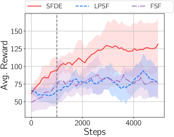
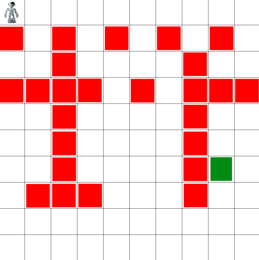
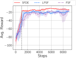
Figure 2: (left) Sample of proposed maze environment with red squares as obstacles with -50 reward and green square as goal with +100 reward. (Right) Obtained results of SFDE and two baselines. The results are averaged over 505050 runs. The dashed vertical line demarcates the adaptation phase.

Theorem 2

Let 𝐒i=1Nsubscript𝐒𝑖1𝑁\bm{\mathrm{S}}_{i=1...N} be N𝑁N different source environments with dissimilar transition functions pi=1Nsubscript𝑝𝑖1𝑁p_{i=1...N}. Let us denote the optimal policy π𝜋\pi that is defined based on the GPI as:

π(s)argmaxa𝒜maxj{1N}Q~𝒯πj(s,a),𝜋𝑠a𝒜argmaxj1Nmaxsuperscriptsubscript~𝑄𝒯superscriptsubscript𝜋𝑗𝑠𝑎\pi(s)\in\mathrm{\underset{a\in\mathcal{A}}{\operatorname*{argmax}\ }\underset{j\in\{1...N\}}{\mathrm{max}}}\ \tilde{Q}_{\mathcal{T}}^{\pi_{j}^{*}}(s,a), (13)

where Q~𝒯πj=(𝝍~πj)T𝐰~𝒯superscriptsubscript~𝑄𝒯superscriptsubscript𝜋𝑗superscriptsuperscriptbold-~𝝍superscriptsubscript𝜋𝑗Tsubscriptbold-~𝐰𝒯\tilde{Q}_{\mathcal{T}}^{\pi_{j}^{*}}=\big{(}\bm{\tilde{\psi}}^{\pi_{j}^{*}}\big{)}^{\mathrm{T}}\bm{\tilde{\mathrm{w}}}_{\mathcal{T}} being the action-value function of an optimal policy learned in 𝐒jsubscript𝐒𝑗\bm{\mathrm{S}}_{j} and executed in target environment 𝒯𝒯\mathcal{T}, 𝝍~πjsuperscriptbold-~𝝍superscriptsubscript𝜋𝑗\bm{\tilde{\psi}}^{\pi_{j}^{*}} is the estimated successor feature from the combined source and target observations from 𝐒jsubscript𝐒𝑗{\bf S}_{j} and 𝒯𝒯\mathcal{T} as defined in Eq. (9), and 𝒘~𝒯subscriptbold-~𝒘𝒯\bm{\tilde{w}}_{\mathcal{T}} is the estimated reward mapper for target environment from Eq. (6). Considering Lemma 1 and Eq. (17), the difference of optimal action-value function in the target environment and our GPI-derived action value function is upper bounded as:

Q𝒯(s,a)Q~𝒯ππj(s,a)superscriptsubscript𝑄𝒯𝑠𝑎superscriptsubscript~𝑄𝒯𝜋superscriptsubscript𝜋𝑗𝑠𝑎\displaystyle Q_{\mathcal{T}}^{*}(s,a)-\tilde{Q}_{\mathcal{T}}^{\pi\in\pi_{j}^{*}}(s,a) 2ϕmax1γ𝐰~𝒯𝐰jabsent2subscriptitalic-ϕmax1𝛾normsubscript~𝐰𝒯subscript𝐰𝑗\displaystyle\leq\frac{2\phi_{\mathrm{max}}}{1-\gamma}\Big{|}\Big{|}{\bf\tilde{w}}_{\mathcal{T}}-{\bf w}_{j}\Big{|}\Big{|}
+\displaystyle+ γ𝐏𝒯(s,a)𝐏j(s,a)(1γ)𝛾normsubscript𝐏𝒯𝑠𝑎subscript𝐏𝑗𝑠𝑎1𝛾\displaystyle\frac{\gamma\Big{|}\Big{|}{\bf P}_{\mathcal{T}}(s,a)-{\bf P}_{j}(s,a)\Big{|}\Big{|}}{(1-\gamma)}
×\displaystyle\times (𝐐𝒯𝐐jj+𝐐jj𝐐𝒯j)(1γ)normsuperscriptsubscript𝐐𝒯superscriptsubscript𝐐𝑗𝑗normsuperscriptsubscript𝐐𝑗𝑗superscriptsubscript𝐐𝒯𝑗1𝛾\displaystyle\frac{\Big{(}\Big{|}\Big{|}{\bf Q}_{\mathcal{T}}^{*}-{\bf Q}_{j}^{j}\Big{|}\Big{|}+\Big{|}\Big{|}{\bf Q}_{j}^{j}-{\bf Q}_{\mathcal{T}}^{j}\Big{|}\Big{|}\Big{)}}{(1-\gamma)}
+\displaystyle+ 2ε(m)(1γ).2𝜀𝑚1𝛾\displaystyle\frac{2\varepsilon(m)}{(1-\gamma)}. (14)

where ϕmax=maxs,aϕ(s,a)subscriptitalic-ϕmaxsubscriptmax𝑠𝑎normitalic-ϕ𝑠𝑎\phi_{\mathrm{max}}=\mathrm{max}_{s,a}||\phi(s,a)||. We also define 𝐏𝒯=[p𝒯(s|s,a),]s𝒮subscript𝐏𝒯subscriptsubscript𝑝𝒯conditionalsuperscript𝑠𝑠𝑎for-allsuperscript𝑠𝒮{\bf P}_{\mathcal{T}}=[p_{\mathcal{T}}(s^{\prime}|s,a),...]_{\forall s^{\prime}\in\mathcal{S}}, 𝐏j=[pj(s|s,a),]s𝒮,subscript𝐏𝑗subscriptsubscript𝑝𝑗conditionalsuperscript𝑠𝑠𝑎for-allsuperscript𝑠𝒮{\bf P}_{j}=[p_{j}(s^{\prime}|s,a),...]_{\forall s^{\prime}\in\mathcal{S}}, 𝐐𝒯=[maxb𝒜Q𝒯(s,b),]s𝒮,superscriptsubscript𝐐𝒯subscript𝑏𝒜maxsuperscriptsubscript𝑄𝒯superscript𝑠𝑏for-allsuperscript𝑠𝒮{\bf Q}_{\mathcal{T}}^{*}=[\underset{b\in\mathcal{A}}{\mathrm{max}}{Q}_{\mathcal{T}}^{*}(s^{\prime},b),...]_{\forall s^{\prime}\in\mathcal{S}}, 𝐐jj=[maxb𝒜Q~jπj(s,b),]s𝒮superscriptsubscript𝐐𝑗𝑗subscript𝑏𝒜maxsuperscriptsubscript~𝑄𝑗superscriptsubscript𝜋𝑗superscript𝑠𝑏for-allsuperscript𝑠𝒮{\bf Q}_{j}^{j}=[\underset{b\in\mathcal{A}}{\mathrm{max}}{\tilde{Q}}_{j}^{\pi_{j}^{*}}(s^{\prime},b),...]_{\forall s^{\prime}\in\mathcal{S}}, 𝐐𝒯j=[maxb𝒜Q~𝒯πj(s,b),]s𝒮superscriptsubscript𝐐𝒯𝑗subscript𝑏𝒜maxsuperscriptsubscript~𝑄𝒯superscriptsubscript𝜋𝑗superscript𝑠𝑏for-allsuperscript𝑠𝒮{\bf Q}_{\mathcal{T}}^{j}=[\underset{b\in\mathcal{A}}{\mathrm{max}}{\tilde{Q}}_{\mathcal{T}}^{\pi_{j}^{*}}(s^{\prime},b),...]_{\forall s^{\prime}\in\mathcal{S}}, and γ𝛾\gamma as the discount factor.

Proof: Proof is available in supplementary material.

In inequality (18), 𝐰~𝒯𝐰jnormsubscript~𝐰𝒯subscript𝐰𝑗\Big{|}\Big{|}{\bf\tilde{w}}_{\mathcal{T}}-{\bf w}_{j}\Big{|}\Big{|} encodes the dissimilarity of reward functions in target environment 𝒯𝒯\mathcal{T} and 𝐒jsubscript𝐒𝑗{\bf S}_{j}, and ε(m)𝜀𝑚\varepsilon(m) holds the error of action-value reconstruction by GP-modelled successor features (Lemma 1). Additionally, γ𝐏𝒯𝐏j×(𝐐𝒯𝐐jj+𝐐jj𝐐𝒯j)/(1γ)𝛾normsubscript𝐏𝒯subscript𝐏𝑗normsuperscriptsubscript𝐐𝒯superscriptsubscript𝐐𝑗𝑗normsuperscriptsubscript𝐐𝑗𝑗superscriptsubscript𝐐𝒯𝑗1𝛾\gamma||{\bf P}_{\mathcal{T}}-{\bf P}_{j}||\times(||{\bf Q}_{\mathcal{T}}^{*}-{\bf Q}_{j}^{j}||+||{\bf Q}_{j}^{j}-{\bf Q}_{\mathcal{T}}^{j}||)/(1-\gamma) is a term related to both the dissimilarity of dynamics in environment j{1,.N}j\in\{1,\ldots.N\} and the target environment 𝒯𝒯\mathcal{T}, as well as the expected future reward in these two environments. We note that Eq. (17) enforces the selection of the best policy among j{1,.N}j\in\{1,\ldots.N\} policies, hence the derived upper bound is only based on the best selected policy among N𝑁N source environments.

Theorem 2 is the core of our theoretical analysis that shows by using N𝑁N different action-value functions that are obtained by their corresponding successor feature functions and reward mapper weights, one can still hold an upper bound on the difference of the optimal policy Q𝒯(s,a)superscriptsubscript𝑄𝒯𝑠𝑎Q_{\mathcal{T}}^{*}(s,a), and Q~𝒯π(s,a)superscriptsubscript~𝑄𝒯𝜋𝑠𝑎\tilde{Q}_{\mathcal{T}}^{\pi}(s,a), if π(s)𝜋𝑠\pi(s) is selected by GPI as defined in Eq. (17). As expected, this upper bound is looser when the norm distance between 𝐰~𝒯subscript~𝐰𝒯{\bf\tilde{w}}_{\mathcal{T}} and 𝐰jsubscript𝐰𝑗{\bf w}_{j} are higher - i.e. the reward functions are significantly different. As explained in Lemma 1, by increasing the amount of noise when modeling the source successor feature functions, σm,d(𝐱)subscript𝜎𝑚𝑑𝐱\sigma_{m,d}({\bf x}) will be higher and accordingly the upper bound will become looser since ε(m)𝜀𝑚\varepsilon(m) increases. This is reasonable as increasing σ𝐒subscript𝜎𝐒\sigma_{\mathbf{S}} indicates that source and target environment are significantly dissimilar. Note that if the environments are exactly similar, γ𝐏𝒯𝐏j×(𝐐𝒯𝐐jj+𝐐jj𝐐𝒯j)/(1γ)=0𝛾normsubscript𝐏𝒯subscript𝐏𝑗normsuperscriptsubscript𝐐𝒯superscriptsubscript𝐐𝑗𝑗normsuperscriptsubscript𝐐𝑗𝑗superscriptsubscript𝐐𝒯𝑗1𝛾0\gamma||{\bf P}_{\mathcal{T}}-{\bf P}_{j}||\times(||{\bf Q}_{\mathcal{T}}^{*}-{\bf Q}_{j}^{j}||+||{\bf Q}_{j}^{j}-{\bf Q}_{\mathcal{T}}^{j}||)/(1-\gamma)=0, this leads to a similar upper bound in (Barreto et al., 2018). Further analysis on the obtained upper bound can be found in supplementary materials.

4 Experiments

We evaluate the performance of our method on 3 benchmarks: (1) A toy navigation problem, (2) Classic CartPole control, and (3) The environment introduced by Barreto et al. (Barreto et al., 2020, 2019). We compare our approach, Successor Features for Dissimilar Environments (SFDE) with two related studies: Fast Successor Features (FSF) (Barreto et al., 2020) and Linear Projection of Successor Features (LPSF) (Zhang et al., 2017). Additional experiments are available in the supplementary materials. All the algorithms, including SFDE, are used in two phases: (1) The first phase is adaptation where we fine-tune the source successor feature functions using the first 100010001000 target observations. This step is method specific. (2) A testing phase in which we only use the learnt policy and collect reward without updating the models. For the adaptation phase, ϵitalic-ϵ\epsilon-greedy based exploration is used, afterwards we set the exploration rate εe=0subscript𝜀𝑒0\varepsilon_{e}=0 in the testing phase to demonstrate the effects of transfer from previous environments. The baseline FSF is not equipped to handle environments with dissimilar dynamics. We adapt this approach by fine-tuning the successor feature functions of the source environments using the first stored 100010001000 observations of the target environment in the adaptation phase. A batch size of 646464 is used at every step 64t100064𝑡100064\leq t\leq 1000 to feed the new target observations to the previously learned source successor features. Once the testing phase starts (t>1000𝑡1000t>1000), we stop fine-tuning of the successor models for the rest of the experiment. For the LPSF baseline, we follow the idea of (Zhang et al., 2017) by defining a linear relation between the source and target successor feature - that is there exists a mapping 𝜷𝜷\bm{\beta}=𝜷1𝜷Nsubscript𝜷1subscript𝜷𝑁\bm{\beta}_{1}...\bm{\beta}_{N} such that the following loss function is minimised: 𝜷(𝜽β)=i=1Nψ~𝒯(𝐱)𝜷iψ~𝐒i(𝐱),𝐱𝒟𝓣formulae-sequencesubscript𝜷subscript𝜽𝛽subscript𝑖1𝑁normsuperscript~𝜓𝒯𝐱subscript𝜷𝑖superscript~𝜓subscript𝐒𝑖𝐱for-all𝐱superscript𝒟𝓣\mathcal{L}_{\bm{\beta}}(\bm{\theta}_{\beta})=\sum_{i=1...N}\Big{|}\Big{|}\tilde{\psi}^{\mathcal{T}}(\bm{\mathrm{x}})-\bm{\beta}_{i}\tilde{\psi}^{\bm{\mathrm{S}}_{i}}(\bm{\mathrm{x}})\Big{|}\Big{|},\forall\bm{\mathrm{x}}\in\mathcal{D^{\bm{T}}}. Intuitively, the best linear projection is found for each source successor feature function to minimise its distance to the target successor. We follow the same approach explained for FSF to feed the target observations in adaptation phase to N𝑁N neural networks that each represent the model of ilimit-from𝑖i-th source successor features i={1,,N}𝑖1𝑁i=\{1,\ldots,N\} with 𝜷subscript𝜷\mathcal{L}_{\bm{\beta}} loss function. Each of these N𝑁N neural networks are MLPs with no hidden layers that is an equivalent of linear regression in which the weights of the neural networks are 𝜷isubscript𝜷𝑖\bm{\beta}_{i}. Likewise, the best obtained value of 𝜷𝜷\bm{\beta} in the adaptation phase is used in the testing phase. We used the same batch size of 646464 to minimise 𝜷subscript𝜷\mathcal{L}_{\bm{\beta}} loss function for LPSF. The linearly projected successor features then used in the GPI framework to obtain the optimal policy. In our approach, we construct the GP based on the combination of source and target observations. To this end, 500500500 randomly sampled observations from source 𝒟𝐒,𝐒{𝐒,,𝐒N}superscript𝒟𝐒for-all𝐒𝐒subscript𝐒𝑁\mathcal{D}^{\mathcal{\mathbf{S}}},\ \forall\mathcal{\mathbf{S}}\in\{{\bf S},\ldots,{\bf S}_{N}\} and all the observations in 𝒟𝓣superscript𝒟𝓣\mathcal{D}^{\bm{\mathcal{T}}} at every step of the adaptation phase is used. However, once the testing phase is initiated, the new target observations are disregarded and previously seen observations from the target are reused. Further details of implementations are available in the supplementary material.

4.1 Toy Navigation Problem

The proposed maze problem consists of a 10×10101010\times 10 grid and the agent needs to find the goal in the maze. The agent can pass through the obstacles but it receives a reward of 5050-50. It also receives 11-1 reward for each step and +100100+100 reward for reaching the goal. The action set is defined as 𝒜={left,right,up,down}𝒜leftrightupdown\mathcal{A}=\{\mathrm{left,right,up,down}\}. Figure 2 (left) shows an example of this environment with red squares indicating obstacles, and the green square as the goal.

A set of 121212 policies Π𝐒={π𝐒1,,π𝐒12}superscriptΠ𝐒superscript𝜋subscript𝐒1superscript𝜋subscript𝐒12\Pi^{\mathrm{\mathbf{S}}}=\big{\{}\pi^{\mathrm{\mathbf{S}}_{1}},\ldots,\pi^{\mathrm{\mathbf{S}}_{12}}\big{\}} is learnt using generic Q-Learning on randomly generated maze source environments {(𝒮,𝒜,p1,R1),,(𝒮,𝒜,p12,R12)}𝒮𝒜subscript𝑝1subscript𝑅1𝒮𝒜subscript𝑝12subscript𝑅12\Big{\{}\mathcal{M}(\mathcal{S},\mathcal{A},p_{1},R_{1}),\ldots,\mathcal{M}(\mathcal{S},\mathcal{A},p_{12},R_{12})\Big{\}} as 𝐒1,,𝐒12subscript𝐒1subscript𝐒12{\bf S}_{1},\ldots,{\bf S}_{12} in which the location of 25 obstacles and goal are changed. After obtaining the corresponding policies, successor feature functions of these source environments are learnt following Algorithm 1. Given 𝝍~π1,,𝝍~π12,superscriptbold-~𝝍subscript𝜋1superscriptbold-~𝝍subscript𝜋12\bm{\tilde{\psi}}^{\pi_{1}},\ldots,\bm{\tilde{\psi}}^{\pi_{12}}, we generate a random target environment and use the first 100010001000 observations of adaptation phase as explained. Following Algorithm 2, 𝒢𝒫112𝒢superscript𝒫112\mathcal{GP}^{1...12} is constructed as each step by fitting both source and target observations. We set σ𝐒2=0.1superscriptsubscript𝜎𝐒20.1\sigma_{{\bf S}}^{2}=0.1 and σ2=0.01superscript𝜎20.01\sigma^{2}=0.01 as the modelling noise and the measurement noise, respectively. Having modelled the successor features, we then perform GPI by using the predicted mean as shown in Eq. (9) and (10). To calculate 𝒘~𝒯subscriptbold-~𝒘𝒯\bm{\tilde{w}}_{\mathcal{T}}, the reward mapper of target environment is calculated by minimising loss function introduced in Eq. (6). Figure 2 (right) shows the performance of our approach and other baselines. As expected, our method incorporating the dissimilarity of environments performs better than the other two related approaches. Figure 2 shows that LPSF adjusts the source successor features but it seems to be slower than SFDE in updating the successor feature functions as a linear projection may not always be found. It can be seen that FSF can update the values of successor features to some extent, however, it seems to be less effective than the other 2 approaches. This can be the result of fine-tuning the successor feature models with significantly different observations that can be an issue in such scenarios. Note that we have not used any visual information in this experiment and the location of agent is translated to (x,y)𝑥𝑦(x,y) in the 10×10101010\times 10 grid.

Refer to caption
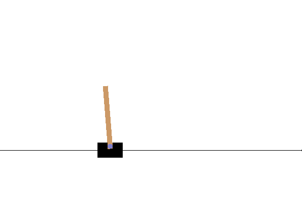
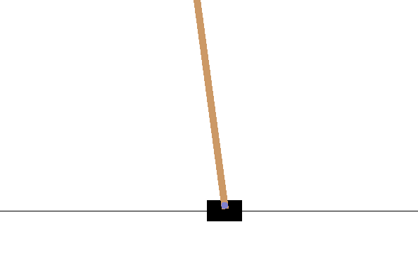
Figure 3: Experiments with CartPole-v0 with Pole_Length=0.5m𝑃𝑜𝑙𝑒_𝐿𝑒𝑛𝑔𝑡0.5𝑚Pole\_Length=0.5m in source environment and Pole_Length=3m𝑃𝑜𝑙𝑒_𝐿𝑒𝑛𝑔𝑡3𝑚Pole\_Length=3m in target environment. The results are averaged over 101010 runs. The dashed vertical line demarcates the adaptation phase.

4.2 CartPole-v0

In the CartPole problem, we define a source environment 𝐒1subscript𝐒1{\bf S}_{1} with a learnt policy π𝐒1superscript𝜋subscript𝐒1\pi^{{\bf S}_{1}} and a target environment 𝒯.𝒯\mathcal{T}. We incorporate the dissimilarities of dynamics in source and target by changing the length of the pole from Pole_Length=0.5m𝑃𝑜𝑙𝑒_𝐿𝑒𝑛𝑔𝑡0.5𝑚Pole\_Length=0.5m in source, to Pole_Length=3.0m𝑃𝑜𝑙𝑒_𝐿𝑒𝑛𝑔𝑡3.0𝑚Pole\_Length=3.0m in the target environment. This change impacts the transition probabilities of the target environment, hence, it can be considered as a change in dynamics. Similar to the previous experiment, we use the first 100010001000 observations in all three methods in a same manner. At each step, we fit 𝒢𝒫1𝒢superscript𝒫1\mathcal{GP}^{1} by combination of source and target observations. We set σ𝐒2=0.1superscriptsubscript𝜎𝐒20.1\sigma_{{\bf S}}^{2}=0.1, σ2=0.01superscript𝜎20.01\sigma^{2}=0.01, and the maximum number of steps in the CartPole is set to 200200200 in each episode. To translate the image data into states that can be used in our framework, we used the flattened output of the last convolution layer as the state of the CartPole environment. The detailed structure of the proposed network is available in supplementary materials. Figure 3 shows the results of this experiment and it can be seen that our proposed method outperforms both FSF and LPSF by using the GP-based modelled successor features.
Refer to caption
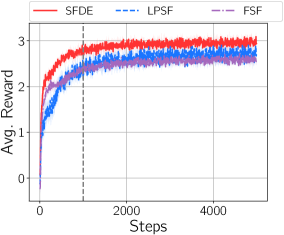
Figure 4: Results on the environment introduced by FSF. The results are averaged over 101010 runs. The dashed vertical line demarcates the adaptation phase.

4.3 FSF Environment

We use the environment introduced in Barreto et al. (Barreto et al., 2020) as our final experiment. The proposed environment is a 10×10101010\times 10 grid cells with 𝒜={left,right,up,down}𝒜leftrightupdown\mathcal{A}=\{\mathrm{left,right,up,down}\}. There are 101010 objects spread across the grid at all time that the agent can pick up. Once an object is picked up, another random object will appear in the grid randomly. Each object belongs to one of two types (red or blue). At each time step, the agent receives an image showing its position, the position of objects, and type of each object (Barreto et al., 2020). Then the agent selects the proper action to move in a direction. The object is assumed picked up, if the agent occupies the cell in which the object presents. In that case, it gets a reward based on the type of the object and a new object will appear randomly in the grid.

Following the setting of FSF experiments, we trained the agent in 222 different source environments with different reward functions and dynamics of the environment. We incorporated the dissimilarity of environments by adding a 5%percent55\% random transition noise to the target environment and creating a single random terminal state with a negative reward of 11-1. Figure 4 shows the obtained results on this problem. Similar to other experiments, our approach seems to outperform the other two baselines. Interestingly, FSF outperforms LPSF in adaptation phase, but both methods approximately converge to the same value of the average reward.

5 Conclusion

In this paper we proposed a novel transfer learning approach based on successor features in RL. Our approach is for the scenarios wherein the source and the target environments have dissimilar reward functions as well as dissimilar environment dynamics. We propose the use of Gaussian Processes to model the source successor features functions as noisy measurements of the target successor functions. We provide a theoretical analysis on the convergence of our method by proving an upper bound on the error of the optimal policy. We evaluate our method on 3 benchmark problems and showed that our method outperform existing methods.

Acknowledgements

This research was partially funded by the Australian Government through the Australian Research Council (ARC). Prof Venkatesh is the recipient of an ARC Australian Laureate Fellowship (FL170100006).

References

  • Ammar & Taylor (2011) Ammar, H. B. and Taylor, M. E. Reinforcement learning transfer via common subspaces. In International Workshop on Adaptive and Learning Agents, pp.  21–36. Springer, 2011.
  • Barreto et al. (2017) Barreto, A., Dabney, W., Munos, R., Hunt, J. J., Schaul, T., van Hasselt, H. P., and Silver, D. Successor features for transfer in reinforcement learning. In Advances in neural information processing systems, pp. 4055–4065, 2017.
  • Barreto et al. (2018) Barreto, A., Borsa, D., Quan, J., Schaul, T., Silver, D., Hessel, M., Mankowitz, D., Zidek, A., and Munos, R. Transfer in deep reinforcement learning using successor features and generalised policy improvement. In International Conference on Machine Learning, pp. 501–510. PMLR, 2018.
  • Barreto et al. (2019) Barreto, A., Borsa, D., Hou, S., Comanici, G., Aygün, E., Hamel, P., Toyama, D., Mourad, S., Silver, D., Precup, D., et al. The option keyboard: Combining skills in reinforcement learning. In Advances in Neural Information Processing Systems, pp. 13052–13062, 2019.
  • Barreto et al. (2020) Barreto, A., Hou, S., Borsa, D., Silver, D., and Precup, D. Fast reinforcement learning with generalized policy updates. Proceedings of the National Academy of Sciences, 117(48):30079–30087, 2020.
  • Dayan (1993) Dayan, P. Improving generalization for temporal difference learning: The successor representation. Neural Computation, 5(4):613–624, 1993.
  • Gupta et al. (2017) Gupta, A., Devin, C., Liu, Y., Abbeel, P., and Levine, S. Learning invariant feature spaces to transfer skills with reinforcement learning. arXiv preprint arXiv:1703.02949, 2017.
  • Joy et al. (2019) Joy, T. T., Rana, S., Gupta, S., and Venkatesh, S. A flexible transfer learning framework for bayesian optimization with convergence guarantee. Expert Systems with Applications, 115:656–672, 2019.
  • Konidaris & Barto (2006) Konidaris, G. and Barto, A. Autonomous shaping: Knowledge transfer in reinforcement learning. In Proceedings of the 23rd international conference on Machine learning, pp.  489–496, 2006.
  • Lederer et al. (2019) Lederer, A., Umlauft, J., and Hirche, S. Uniform error bounds for gaussian process regression with application to safe control. arXiv preprint arXiv:1906.01376, 2019.
  • Liang et al. (2018) Liang, X., Wang, T., Yang, L., and Xing, E. Cirl: Controllable imitative reinforcement learning for vision-based self-driving. In Proceedings of the European Conference on Computer Vision (ECCV), pp.  584–599, 2018.
  • Ma et al. (2020) Ma, C., Ashley, D. R., Wen, J., and Bengio, Y. Universal successor features for transfer reinforcement learning. arXiv preprint arXiv:2001.04025, 2020.
  • Mnih et al. (2015) Mnih, V., Kavukcuoglu, K., Silver, D., Rusu, A. A., Veness, J., Bellemare, M. G., Graves, A., Riedmiller, M., Fidjeland, A. K., Ostrovski, G., et al. Human-level control through deep reinforcement learning. nature, 518(7540):529–533, 2015.
  • Rasmussen (2003) Rasmussen, C. E. Gaussian processes in machine learning. In Summer School on Machine Learning, pp.  63–71. Springer, 2003.
  • Rusu et al. (2016) Rusu, A. A., Rabinowitz, N. C., Desjardins, G., Soyer, H., Kirkpatrick, J., Kavukcuoglu, K., Pascanu, R., and Hadsell, R. Progressive neural networks. arXiv preprint arXiv:1606.04671, 2016.
  • Shilton et al. (2017) Shilton, A., Gupta, S., Rana, S., and Venkatesh, S. Regret bounds for transfer learning in bayesian optimisation. In Artificial Intelligence and Statistics, pp.  307–315. PMLR, 2017.
  • Siriwardhana et al. (2019) Siriwardhana, S., Weerasakera, R., Matthies, D. J., and Nanayakkara, S. Vusfa: Variational universal successor features approximator to improve transfer drl for target driven visual navigation. arXiv preprint arXiv:1908.06376, 2019.
  • Srinivas et al. (2009) Srinivas, N., Krause, A., Kakade, S. M., and Seeger, M. Gaussian process optimization in the bandit setting: No regret and experimental design. arXiv preprint arXiv:0912.3995, 2009.
  • Yin & Pan (2017) Yin, H. and Pan, S. Knowledge transfer for deep reinforcement learning with hierarchical experience replay. In Proceedings of the AAAI Conference on Artificial Intelligence, volume 31, 2017.
  • Zhang et al. (2017) Zhang, J., Springenberg, J. T., Boedecker, J., and Burgard, W. Deep reinforcement learning with successor features for navigation across similar environments. In 2017 IEEE/RSJ International Conference on Intelligent Robots and Systems (IROS), pp.  2371–2378. IEEE, 2017.
  • Zhu et al. (2020) Zhu, Z., Lin, K., and Zhou, J. Transfer learning in deep reinforcement learning: A survey. arXiv preprint arXiv:2009.07888, 2020.

6 Supplementary Materials

6.1 Theoretical Proofs

We show our theoretical analysis for both cases of finite 𝕏𝕏\mathbb{X} and infinite 𝕏𝕏\mathbb{X}.

6.2 Finite 𝕏𝕏\mathbb{X}

Theorem 1

Let 𝐒isubscript𝐒𝑖{\bf S}_{i} and 𝐒jsubscript𝐒𝑗{\bf S}_{j} be two different source environments with dissimilar transition dynamics pisubscript𝑝𝑖p_{i} and pjsubscript𝑝𝑗p_{j} respectively. Let δijmaxs,a|ri(s,a)rj(s,a)|subscript𝛿𝑖𝑗subscriptmax𝑠𝑎subscript𝑟𝑖𝑠𝑎subscript𝑟𝑗𝑠𝑎\delta_{ij}\triangleq\mathrm{max}_{s,a}\ |r_{i}(s,a)-r_{j}(s,a)|, where ri(.,.)r_{i}(.,.) and rj(.,.)r_{j}(.,.) are the reward functions of environment 𝐒isubscript𝐒𝑖{\bf S}_{i} and 𝐒jsubscript𝐒𝑗{\bf S}_{j} respectively. We denote πisuperscriptsubscript𝜋𝑖\pi_{i}^{*} and πjsuperscriptsubscript𝜋𝑗\pi_{j}^{*} as optimal policies in 𝐒isubscript𝐒𝑖{\bf S}_{i} and 𝐒jsubscript𝐒𝑗{\bf S}_{j}. It can be shown that the difference of their action-value functions is upper bounded as:

Qiπi(s,a)Qiπj(s,a)superscriptsubscript𝑄𝑖superscriptsubscript𝜋𝑖𝑠𝑎superscriptsubscript𝑄𝑖superscriptsubscript𝜋𝑗𝑠𝑎\displaystyle{Q}_{i}^{\pi_{i}^{*}}(s,a)-{Q}_{i}^{\pi_{j}^{*}}(s,a) 2δij1γabsent2subscript𝛿𝑖𝑗1𝛾\displaystyle\leq\frac{2\delta_{ij}}{1-\gamma}
+\displaystyle+ γ𝐏i(s,a)𝐏j(s,a)(1γ)𝛾normsubscript𝐏𝑖𝑠𝑎subscript𝐏𝑗𝑠𝑎1𝛾\displaystyle\frac{\gamma\Big{|}\Big{|}{\bf P}_{i}(s,a)-{\bf P}_{j}(s,a)\Big{|}\Big{|}}{(1-\gamma)}
×\displaystyle\times (𝐐ii𝐐jj+𝐐jj𝐐ij)(1γ),normsuperscriptsubscript𝐐𝑖𝑖superscriptsubscript𝐐𝑗𝑗normsuperscriptsubscript𝐐𝑗𝑗superscriptsubscript𝐐𝑖𝑗1𝛾\displaystyle\frac{\Big{(}\Big{|}\Big{|}{\bf Q}_{i}^{i}-{\bf Q}_{j}^{j}\Big{|}\Big{|}+\Big{|}\Big{|}{\bf Q}_{j}^{j}-{\bf Q}_{i}^{j}\Big{|}\Big{|}\Big{)}}{(1-\gamma)}, (15)

where Qiπksuperscriptsubscript𝑄𝑖superscriptsubscript𝜋𝑘{Q}_{i}^{\pi_{k{\bf}}^{*}} shows the action-value function in environment 𝐒isubscript𝐒𝑖{\bf S}_{i} by following an optimal policy that is learned in the environment 𝐒k{𝐒1,,𝐒N}subscript𝐒𝑘subscript𝐒1subscript𝐒𝑁{\bf S}_{k}\in\{{\bf S}_{1},\ldots,{\bf S}_{N}\}. We also define 𝐏i(s,a)=[pi(s|s,a),]s𝒮subscript𝐏𝑖𝑠𝑎subscriptsubscript𝑝𝑖conditionalsuperscript𝑠𝑠𝑎for-allsuperscript𝑠𝒮{\bf P}_{i}(s,a)=[p_{i}(s^{\prime}|s,a),...]_{\forall s^{\prime}\in\mathcal{S}}, 𝐏j(s,a)=[pj(s|s,a),]s𝒮,subscript𝐏𝑗𝑠𝑎subscriptsubscript𝑝𝑗conditionalsuperscript𝑠𝑠𝑎for-allsuperscript𝑠𝒮{\bf P}_{j}(s,a)=[p_{j}(s^{\prime}|s,a),...]_{\forall s^{\prime}\in\mathcal{S}}, 𝐐ii=[maxb𝒜Qiπi(s,b),]s𝒮,superscriptsubscript𝐐𝑖𝑖subscript𝑏𝒜maxsuperscriptsubscript𝑄𝑖superscriptsubscript𝜋𝑖superscript𝑠𝑏for-allsuperscript𝑠𝒮{\bf Q}_{i}^{i}=[\underset{b\in\mathcal{A}}{\mathrm{max}}{Q}_{i}^{\pi_{i}^{*}}(s^{\prime},b),...]_{\forall s^{\prime}\in\mathcal{S}}, 𝐐jj=[maxb𝒜Qjπj(s,b),]s𝒮superscriptsubscript𝐐𝑗𝑗subscript𝑏𝒜maxsuperscriptsubscript𝑄𝑗superscriptsubscript𝜋𝑗superscript𝑠𝑏for-allsuperscript𝑠𝒮{\bf Q}_{j}^{j}=[\underset{b\in\mathcal{A}}{\mathrm{max}}{Q}_{j}^{\pi_{j}^{*}}(s^{\prime},b),...]_{\forall s^{\prime}\in\mathcal{S}}, 𝐐ij=[maxb𝒜Qiπj(s,b),]s𝒮superscriptsubscript𝐐𝑖𝑗subscript𝑏𝒜maxsuperscriptsubscript𝑄𝑖superscriptsubscript𝜋𝑗superscript𝑠𝑏for-allsuperscript𝑠𝒮{\bf Q}_{i}^{j}=[\underset{b\in\mathcal{A}}{\mathrm{max}}{Q}_{i}^{\pi_{j}^{*}}(s^{\prime},b),...]_{\forall s^{\prime}\in\mathcal{S}}, γ𝛾\gamma as the discount factor, and ||.||||.|| to be 2limit-from22-norm (Euclidean norm). Proof: We start by following the steps from (Barreto et al., 2018). The left side of the inequality (15) can be rewritten as:

Qiπi(s,a)Qiπj(s,a)superscriptsubscript𝑄𝑖superscriptsubscript𝜋𝑖𝑠𝑎superscriptsubscript𝑄𝑖superscriptsubscript𝜋𝑗𝑠𝑎\displaystyle{Q}_{i}^{\pi_{i}^{*}}(s,a)-{Q}_{i}^{\pi_{j}^{*}}(s,a) =Qiπi(s,a)Qjπj(s,a)absentsuperscriptsubscript𝑄𝑖superscriptsubscript𝜋𝑖𝑠𝑎superscriptsubscript𝑄𝑗superscriptsubscript𝜋𝑗𝑠𝑎\displaystyle={Q}_{i}^{\pi_{i}^{*}}(s,a)-{Q}_{j}^{\pi_{j}^{*}}(s,a)
+\displaystyle+ Qjπj(s,a)Qiπj(s,a)superscriptsubscript𝑄𝑗superscriptsubscript𝜋𝑗𝑠𝑎superscriptsubscript𝑄𝑖superscriptsubscript𝜋𝑗𝑠𝑎\displaystyle{Q}_{j}^{\pi_{j}^{*}}(s,a)-{Q}_{i}^{\pi_{j}^{*}}(s,a)
\displaystyle\leq |Qiπi(s,a)Qjπj(s,a)|(I)subscriptsuperscriptsubscript𝑄𝑖superscriptsubscript𝜋𝑖𝑠𝑎superscriptsubscript𝑄𝑗superscriptsubscript𝜋𝑗𝑠𝑎(I)\displaystyle\underbrace{\Big{|}{Q}_{i}^{\pi_{i}^{*}}(s,a)-{Q}_{j}^{\pi_{j}^{*}}(s,a)\Big{|}}_{\text{(I)}}
+\displaystyle+ |Qjπj(s,a)Qiπj(s,a)|(II).subscriptsuperscriptsubscript𝑄𝑗superscriptsubscript𝜋𝑗𝑠𝑎superscriptsubscript𝑄𝑖superscriptsubscript𝜋𝑗𝑠𝑎(II)\displaystyle\underbrace{\Big{|}{Q}_{j}^{\pi_{j}^{*}}(s,a)-{Q}_{i}^{\pi_{j}^{*}}(s,a)\Big{|}}_{\text{(II)}}.

For (I), it can be shown that:

|Qiπi(s,a)Qjπj(s,a)||ri(s,a)+γspi(s|s,a)maxsQiπi(s,b)rj(s,a)γspj(s|s,a)maxbQjπj(s,b)||ri(s,a)rj(s,a)|+|γspi(s|s,a)maxbQiπi(s,b)γspj(s|s,a)maxbQjπj(s,b)||ri(s,a)rj(s,a)|+γ(||(𝐏i𝐏j).(𝐐ii𝐐jj)||)|ri(s,a)rj(s,a)|+γ𝐏i𝐏j×𝐐ii𝐐jj=δij+γ𝐏i𝐏j×𝐐ii𝐐jjδij1γ+γ1γ𝐏i𝐏j×𝐐ii𝐐jj,s𝒮\Big{|}{Q}_{i}^{\pi_{i}^{*}}(s,a)-{Q}_{j}^{\pi_{j}^{*}}(s,a)\Big{|}\leq\Big{|}r_{i}(s,a)+\gamma\sum_{s^{\prime}}p_{i}(s^{\prime}|s,a)\\ \underset{}{\mathrm{\underset{s^{\prime}}{\mathrm{max}}}\ {Q}_{i}^{\pi_{i}^{*}}(s^{\prime},b)}-r_{j}(s,a)-\gamma\sum_{s^{\prime}}p_{j}(s^{\prime}|s,a)\underset{}{\mathrm{\underset{b}{\mathrm{max}}}\ {Q}_{j}^{\pi_{j}^{*}}(s^{\prime},b)}\Big{|}\leq\\ \Big{|}r_{i}(s,a)-r_{j}(s,a)\Big{|}+\Big{|}\gamma\sum_{s^{\prime}}p_{i}(s^{\prime}|s,a)\underset{}{\mathrm{\underset{b}{\mathrm{max}}}\ {Q}_{i}^{\pi_{i}^{*}}(s^{\prime},b)}-\\ \gamma\sum_{s^{\prime}}p_{j}(s^{\prime}|s,a)\underset{}{\mathrm{\underset{b}{\mathrm{max}}}\ {Q}_{j}^{\pi_{j}^{*}}(s^{\prime},b)}\Big{|}\leq\\ \Big{|}r_{i}(s,a)-r_{j}(s,a)\Big{|}+\gamma\Big{(}\Big{|}\Big{|}\big{(}{\bf P}_{i}-{\bf P}_{j}\big{)}.\big{(}{\bf Q}_{i}^{i}-{\bf Q}_{j}^{j}\big{)}\Big{|}\Big{|}\Big{)}\leq\\ \Big{|}r_{i}(s,a)-r_{j}(s,a)\Big{|}+\gamma\Big{|}\Big{|}{\bf P}_{i}-{\bf P}_{j}\Big{|}\Big{|}\times\Big{|}\Big{|}{\bf Q}_{i}^{i}-{\bf Q}_{j}^{j}\Big{|}\Big{|}=\\ \delta_{ij}+\gamma\Big{|}\Big{|}{\bf P}_{i}-{\bf P}_{j}\Big{|}\Big{|}\times\Big{|}\Big{|}{\bf Q}_{i}^{i}-{\bf Q}_{j}^{j}\Big{|}\Big{|}\leq\\ \frac{\delta_{ij}}{1-\gamma}+\frac{\gamma}{1-\gamma}\Big{|}\Big{|}{\bf P}_{i}-{\bf P}_{j}\Big{|}\Big{|}\times\Big{|}\Big{|}{\bf Q}_{i}^{i}-{\bf Q}_{j}^{j}\Big{|}\Big{|},\ \forall s^{\prime}\in\mathcal{S}

For (II), it can be shown that:

|Qjπj(s,a)Qiπj(s,a)||rj(s,a)+γspj(s|s,a)maxbQjπj(s,b)ri(s,a)γspi(s|s,a)maxbQiπj(s,b)||rj(s,a)ri(s,a)|+|γspj(s|s,a)maxbQjπj(s,b)γspi(s|s,a)maxbQiπj(s,b)||rj(s,a)ri(s,a)|+γ(||(𝐏j𝐏i).(𝐐jj𝐐ij)||)|rj(s,a)ri(s,a)|+γ𝐏j𝐏i×𝐐jj𝐐ij=δij+γ𝐏j𝐏i×𝐐jj𝐐ijδij1γ+γ1γ𝐏j𝐏i×𝐐jj𝐐ij=δij1γ+γ1γ𝐏i𝐏j×𝐐jj𝐐ij,s𝒮\Big{|}{Q}_{j}^{\pi_{j}^{*}}(s,a)-{Q}_{i}^{\pi_{j}^{*}}(s,a)\Big{|}\leq\Big{|}r_{j}(s,a)+\gamma\sum_{s^{\prime}}p_{j}(s^{\prime}|s,a)\\ \underset{}{\mathrm{\underset{b}{\mathrm{max}}}\ {Q}_{j}^{\pi_{j}^{*}}(s^{\prime},b)}-r_{i}(s,a)-\gamma\sum_{s^{\prime}}p_{i}(s^{\prime}|s,a)\underset{}{\mathrm{\underset{b}{\mathrm{max}}}\ {Q}_{i}^{\pi_{j}^{*}}(s^{\prime},b)}\Big{|}\leq\\ \Big{|}r_{j}(s,a)-r_{i}(s,a)\Big{|}+\Big{|}\gamma\sum_{s^{\prime}}p_{j}(s^{\prime}|s,a)\underset{}{\mathrm{\underset{b}{\mathrm{max}}}\ {Q}_{j}^{\pi_{j}^{*}}(s^{\prime},b)}-\\ \gamma\sum_{s^{\prime}}p_{i}(s^{\prime}|s,a)\underset{}{\mathrm{\underset{b}{\mathrm{max}}}\ {Q}_{i}^{\pi_{j}^{*}}(s^{\prime},b)}\Big{|}\leq\\ \Big{|}r_{j}(s,a)-r_{i}(s,a)\Big{|}+\gamma\Big{(}\Big{|}\Big{|}\big{(}{\bf P}_{j}-{\bf P}_{i}\big{)}.\big{(}{\bf Q}_{j}^{j}-{\bf Q}_{i}^{j}\big{)}\Big{|}\Big{|}\Big{)}\leq\\ \Big{|}r_{j}(s,a)-r_{i}(s,a)\Big{|}+\gamma\Big{|}\Big{|}{\bf P}_{j}-{\bf P}_{i}\Big{|}\Big{|}\times\Big{|}\Big{|}{\bf Q}_{j}^{j}-{\bf Q}_{i}^{j}\Big{|}\Big{|}=\\ \delta_{ij}+\gamma\Big{|}\Big{|}{\bf P}_{j}-{\bf P}_{i}\Big{|}\Big{|}\times\Big{|}\Big{|}{\bf Q}_{j}^{j}-{\bf Q}_{i}^{j}\Big{|}\Big{|}\leq\\ \frac{\delta_{ij}}{1-\gamma}+\frac{\gamma}{1-\gamma}\Big{|}\Big{|}{\bf P}_{j}-{\bf P}_{i}\Big{|}\Big{|}\times\Big{|}\Big{|}{\bf Q}_{j}^{j}-{\bf Q}_{i}^{j}\Big{|}\Big{|}=\\ \frac{\delta_{ij}}{1-\gamma}+\frac{\gamma}{1-\gamma}\Big{|}\Big{|}{\bf P}_{i}-{\bf P}_{j}\Big{|}\Big{|}\times\Big{|}\Big{|}{\bf Q}_{j}^{j}-{\bf Q}_{i}^{j}\Big{|}\Big{|},\ \forall s^{\prime}\in\mathcal{S}

Considering (I) and (II), it leads to the upper bound:

Qiπi(s,a)Qiπj(s,a)superscriptsubscript𝑄𝑖superscriptsubscript𝜋𝑖𝑠𝑎superscriptsubscript𝑄𝑖superscriptsubscript𝜋𝑗𝑠𝑎\displaystyle{Q}_{i}^{\pi_{i}^{*}}(s,a)-{Q}_{i}^{\pi_{j}^{*}}(s,a) 2δij1γ+γ𝐏i𝐏j(1γ)absent2subscript𝛿𝑖𝑗1𝛾𝛾normsubscript𝐏𝑖subscript𝐏𝑗1𝛾\displaystyle\leq\frac{2\delta_{ij}}{1-\gamma}+\frac{\gamma\Big{|}\Big{|}{\bf P}_{i}-{\bf P}_{j}\Big{|}\Big{|}}{(1-\gamma)}
×\displaystyle\times (𝐐ii𝐐jj+𝐐jj𝐐ij)(1γ).normsuperscriptsubscript𝐐𝑖𝑖superscriptsubscript𝐐𝑗𝑗normsuperscriptsubscript𝐐𝑗𝑗superscriptsubscript𝐐𝑖𝑗1𝛾\displaystyle\frac{\Big{(}\Big{|}\Big{|}{\bf Q}_{i}^{i}-{\bf Q}_{j}^{j}\Big{|}\Big{|}+\Big{|}\Big{|}{\bf Q}_{j}^{j}-{\bf Q}_{i}^{j}\Big{|}\Big{|}\Big{)}}{(1-\gamma)}.
\displaystyle\ \ \ \ \!\ \ \ \ \ \ \ \!\ \ \ \ \ \ \ \ \ \ \ \ \ \ \ \ \ \ \ \ \ \ \ \ \ \ \ \ \spadesuit

Lemma 1

Let π1,,πNsuperscriptsubscript𝜋1superscriptsubscript𝜋𝑁\pi_{1}^{*},...,\pi_{N}^{*} be N𝑁N optimal policies for 𝐒1,,𝐒Nsubscript𝐒1subscript𝐒𝑁{\bf S}_{1},\ldots,{\bf S}_{N} respectively and Q~𝒯πj=(𝝍~πj)T𝐰~𝒯superscriptsubscript~𝑄𝒯superscriptsubscript𝜋𝑗superscriptsuperscriptbold-~𝝍superscriptsubscript𝜋𝑗Tsubscriptbold-~𝐰𝒯\tilde{Q}_{\mathcal{T}}^{\pi_{j}^{*}}=\big{(}\bm{\tilde{\psi}}^{\pi_{j}^{*}}\big{)}^{\mathrm{T}}\bm{\tilde{\mathrm{w}}}_{\mathcal{T}} denote the action-value function of an optimal policy learned in 𝐒jsubscript𝐒𝑗\bm{\mathrm{S}}_{j} and executed in the target environment 𝒯𝒯\mathcal{T}. Let 𝝍~πjsuperscriptbold-~𝝍superscriptsubscript𝜋𝑗\bm{\tilde{\psi}}^{\pi_{j}^{*}} denote the estimated successor feature function from the combined source and target observations from 𝐒jsubscript𝐒𝑗{\bf S}_{j} and 𝒯𝒯\mathcal{T} as defined in Eq. (9)(in paper), and 𝐰~𝒯subscriptbold-~𝐰𝒯\bm{\mathrm{\tilde{w}}}_{\mathcal{T}} is the estimated reward mapper for environment 𝒯𝒯\mathcal{T} by using loss function in Eq. (6)(in paper). It can be shown that the difference of the true action-value function and the estimated one through successor feature functions and reward mapper, is bounded as:

Pr(|Q𝒯πj(s,a)Q~𝒯πj(s,a)|ε(m)s,a)1δ,Prsuperscriptsubscript𝑄𝒯superscriptsubscript𝜋𝑗𝑠𝑎superscriptsubscript~𝑄𝒯superscriptsubscript𝜋𝑗𝑠𝑎𝜀𝑚for-all𝑠𝑎1𝛿\mathrm{Pr}\Big{(}\Big{|}{Q_{\mathcal{T}}}^{\pi_{j}^{*}}(s,a)-\tilde{Q}_{\mathcal{T}}^{\pi_{j}^{*}}(s,a)\Big{|}\leq\varepsilon(m)\ \forall s,a\Big{)}\geq 1-\delta,

where ε(m)=2log(|𝕏|um/δ)σm,d(𝐱),𝐱𝕏δ(0,1)formulae-sequence𝜀𝑚2log𝕏subscript𝑢𝑚𝛿subscript𝜎𝑚𝑑𝐱𝐱𝕏𝛿01\varepsilon(m)=\sqrt{2\mathrm{log}(|\mathbb{X}|u_{m}/\delta)}\sigma_{m,d}({\bf x}),\ {\bf x\in\mathbb{X}}\ \delta\in(0,1), um=π2m26subscript𝑢𝑚superscript𝜋2superscript𝑚26u_{m}=\frac{\pi^{2}m^{2}}{6}, m𝑚m being the number of observations in environment 𝒯𝒯\mathcal{T}, and 𝐱=(s,a)𝐱𝑠𝑎{\bf x}=(s,a). σm,d(𝐱)subscript𝜎𝑚𝑑𝐱\sigma_{m,d}({\bf x}) is the square root of posterior variance as defined in Eq. (10)(in paper).

Proof: For proving this Lemma, we first follow the properties of Normal distribution. Let us assume that l𝒩(0,1),similar-to𝑙𝒩01l\sim\mathcal{N}(0,1), and ψ𝒯,dπj(𝐱)𝒩(μm,d(𝐱),σm,d2(𝐱))similar-tosuperscriptsubscript𝜓𝒯𝑑superscriptsubscript𝜋𝑗𝐱𝒩subscript𝜇𝑚𝑑𝐱superscriptsubscript𝜎𝑚𝑑2𝐱{\psi_{\mathcal{T},d}^{\pi_{j}^{*}}}({\bf x})\sim\mathcal{N}\big{(}\mu_{m,d}({\bf x}),\sigma_{m,d}^{2}({\bf x})\big{)}, 𝐱𝕏,𝐱𝕏{\bf x}\in\mathbb{X}, 𝐱=(s,a)𝐱𝑠𝑎\mathrm{{\bf x}}=(s,a), and d={1,,D}𝑑1𝐷d=\{1,\ldots,D\} as defined in Eq. (9) and Eq. (10)(in paper). m𝑚m target observations are assumed to be available. We follow (Srinivas et al., 2009), based on the properties of Normal distribution, Pr(l>c),c>0Pr𝑙𝑐𝑐0\mathrm{Pr}(l>c),\ c>0 is calculated as:

Pr(l\displaystyle\mathrm{Pr}(l >c)=ec2/2(2π)1/2e(lc)2c(lc)dl\displaystyle>c)=e^{-c^{2}/2}(2\pi)^{-1/2}\int e^{-(l-c)^{2}-c(l-c)}dl\leq
ec2/2superscript𝑒superscript𝑐22\displaystyle e^{-c^{2}/2} Pr(l>0)=12(ec2/2).Pr𝑙012superscript𝑒superscript𝑐22\displaystyle\mathrm{Pr}(l>0)=\frac{1}{2}(e^{-c^{2}/2}).

As c>0𝑐0c>0, we know ec(lc)1superscript𝑒𝑐𝑙𝑐1e^{-c(l-c)}\leq 1 for lc.𝑙𝑐l\geq c. Accordingly, Pr[|ψ𝒯,dπj(𝐱)ψ~𝒯,dπj(𝐱)|>βm1/2σm,d(𝐱)]eβm/2,βm=2log(|𝕏|um/δ).formulae-sequencePrdelimited-[]superscriptsubscript𝜓𝒯𝑑superscriptsubscript𝜋𝑗𝐱superscriptsubscript~𝜓𝒯𝑑superscriptsubscript𝜋𝑗𝐱superscriptsubscript𝛽𝑚12subscript𝜎𝑚𝑑𝐱superscript𝑒subscript𝛽𝑚2subscript𝛽𝑚2log𝕏subscript𝑢𝑚𝛿\mathrm{Pr}\Big{[}|{\psi_{\mathcal{T},d}^{\pi_{j}^{*}}}(\mathrm{{\bf x}})-\tilde{\psi}_{\mathcal{T},d}^{\pi_{j}^{*}}(\mathrm{{\bf x}})|>\beta_{m}^{1/2}\sigma_{m,d}(\mathrm{{\bf x}})\Big{]}\leq e^{-\beta_{m}/2},\ \beta_{m}=2\mathrm{log}(|\mathbb{X}|u_{m}/\delta). Now assuming l=(ψ𝒯,dπj(𝐱)ψ~𝒯,dπj(𝐱))/σm,d(𝐱)𝑙superscriptsubscript𝜓𝒯𝑑superscriptsubscript𝜋𝑗𝐱superscriptsubscript~𝜓𝒯𝑑superscriptsubscript𝜋𝑗𝐱subscript𝜎𝑚𝑑𝐱l=\big{(}{\psi_{\mathcal{T},d}^{\pi_{j}^{*}}}(\mathrm{{\bf x}})-\tilde{\psi}_{\mathcal{T},d}^{\pi_{j}^{*}}(\mathrm{{\bf x}})\big{)}/\sigma_{m,d}(\mathrm{{\bf x}}) and c=βm1/2𝑐superscriptsubscript𝛽𝑚12c=\beta_{m}^{1/2}, the error of modelling successor feature function can be written as:

Pr(|ψ𝒯,dπj(𝐱)ψ~𝒯,dπj(s,a)|\displaystyle\mathrm{Pr}\Big{(}\Big{|}{\psi_{\mathcal{T},d}^{\pi_{j}^{*}}}(\mathrm{{\bf x}})-\tilde{\psi}_{\mathcal{T},d}^{\pi_{j}^{*}}(s,a)\Big{|} βm1/2σm,d(𝐱))\displaystyle\leq\beta_{m}^{1/2}\sigma_{m,d}(\mathrm{{\bf x}})\Big{)}
\displaystyle\geq 1|𝕏|eβm/2.𝐱𝕏.\displaystyle 1-|\mathbb{X}|e^{-\beta_{m}/2}.\ \ \forall\mathrm{\mathrm{{\bf x}}}\in\mathbb{X}. (16)

If |𝕏|eβm/2=δum𝕏superscript𝑒subscript𝛽𝑚2𝛿subscript𝑢𝑚|\mathbb{X}|e^{-\beta_{m}/2}=\frac{\delta}{u_{m}}, the inequality 16 holds for um=π2m2/6subscript𝑢𝑚superscript𝜋2superscript𝑚26u_{m}=\pi^{2}m^{2}/6. We follow the assumption in (Barreto et al., 2017, 2019, 2020), 𝐰~𝒯,s.t.Q~𝒯πj=(𝝍~πj)T𝐰~𝒯formulae-sequencesubscriptbold-~𝐰𝒯𝑠𝑡superscriptsubscript~𝑄𝒯superscriptsubscript𝜋𝑗superscriptsuperscriptbold-~𝝍superscriptsubscript𝜋𝑗Tsubscriptbold-~𝐰𝒯\exists\bm{\tilde{\mathrm{w}}}_{\mathcal{T}},\ s.t.\ \tilde{Q}_{\mathcal{T}}^{\pi_{j}^{*}}=\big{(}\bm{\tilde{\psi}}^{\pi_{j}^{*}}\big{)}^{\mathrm{T}}\bm{\tilde{\mathrm{w}}}_{\mathcal{T}} given all dimensions of successor feature function, hence Lemma 1 holds for 𝐱𝕏::for-all𝐱𝕏absent\forall\mathrm{{\bf x}}\in\mathbb{X}:

Pr(|Q𝒯πj(𝐱)Q~𝒯πj(𝐱)|\displaystyle\mathrm{Pr}\Big{(}\Big{|}{Q_{\mathcal{T}}}^{\pi_{j}^{*}}(\mathrm{{\bf x}})-\tilde{Q}_{\mathcal{T}}^{\pi_{j}^{*}}(\mathrm{{\bf x}})\Big{|} ε(m)𝐱𝕏)1δ.\displaystyle\leq\varepsilon(m)\ \forall\mathrm{{\bf x}}\in\mathbb{X}\Big{)}\geq 1-\delta.
\displaystyle\ \ \ \ \!\ \ \ \ \ \ \ \!\ \ \ \ \ \ \ \ \ \ \spadesuit

We note ε(m)𝜀𝑚\varepsilon(m) decreases ε(m)(𝒪log(m)1)𝜀𝑚𝒪logsuperscript𝑚1\varepsilon(m)\in\big{(}\mathcal{O}\mathrm{log}(m)^{-1}\big{)} as σm,d(𝐱)𝒪(log(m)2)subscript𝜎𝑚𝑑𝐱𝒪logsuperscript𝑚2\sigma_{m,d}({\bf x})\in\mathcal{O}\big{(}\mathrm{log}(m)^{-2}\big{)} (Lederer et al., 2019) and 2log(|𝕏|um/δ)𝒪(log(m))2log𝕏subscript𝑢𝑚𝛿𝒪log𝑚\sqrt{2\mathrm{log}(|\mathbb{X}|u_{m}/\delta)}\in\mathcal{O}\big{(}\mathrm{log}(m)\big{)}. This guarantees that the error of modelling convergence to zero as m𝑚m\rightarrow\infty. Before starting the proof of Theorem 2, we present Remark 1 based on the concept of GPI (Barreto et al., 2018) as follows:

Remark 1

Let π1,,πNsubscript𝜋1subscript𝜋𝑁\pi_{1},...,\pi_{N} be N𝑁N decision policies and correspondingly Q~π1,Q~π2,,Q~πNsuperscript~𝑄subscript𝜋1superscript~𝑄subscript𝜋2superscript~𝑄subscript𝜋𝑁\tilde{Q}^{\pi_{1}},\tilde{Q}^{\pi_{2}},...,\tilde{Q}^{\pi_{N}} are the respective estimated action-value functions (Lemma 1) such that:

|Qπi(𝐱)Q~πi(𝐱)|ε(m)𝐱=(s,a),formulae-sequencesuperscript𝑄subscript𝜋𝑖𝐱superscript~𝑄subscript𝜋𝑖𝐱𝜀𝑚for-all𝐱𝑠𝑎\Big{|}{Q}^{\pi_{i}}(\bm{\mathrm{x}})-\tilde{Q}^{\pi_{i}}(\bm{\mathrm{x}})\Big{|}\leq\varepsilon(m)\ \ \forall\bm{\mathrm{x}}=(s,a),

where m𝑚m is the number of target observations. Defining: π(s)argmaxamaxiQ~πi(s,a)𝜋𝑠subscriptargmaxasubscriptmaxisuperscript~𝑄subscript𝜋𝑖𝑠𝑎\pi(s)\in\mathrm{argmax_{a}\ max_{i}}\ \tilde{Q}^{\pi_{i}}(s,a), Then:

Qπ(𝐱)max𝑖Qπi(𝐱)21γε(m)𝐱=(s,a).formulae-sequencesuperscript𝑄𝜋𝐱𝑖maxsuperscript𝑄subscript𝜋𝑖𝐱21𝛾𝜀𝑚for-all𝐱𝑠𝑎{Q}^{\pi}(\bm{\mathrm{x}})\geq\underset{i}{\mathrm{max}}\ {Q}^{\pi_{i}}(\bm{\mathrm{x}})-\frac{2}{1-\gamma}\varepsilon(m)\ \ \forall\bm{\mathrm{x}}=(s,a).

Proof:

We start the proof by extending PπmaxiQ~πi(s,a)superscript𝑃𝜋imaxsuperscript~𝑄subscript𝜋𝑖𝑠𝑎P^{\pi}\mathrm{\underset{i}{\mathrm{max}}}\ {\tilde{Q}}^{\pi_{i}}(s,a), where Pπsuperscript𝑃𝜋P^{\pi} is the Bellman operator (Barreto et al., 2018):

PπmaxiQ~πi(s,a)=r(s,a)+γspi(s|s,a)maxiQ~πi(s,π(s))r(s,a)+γspi(s|s,a)maxbQπi(s,b)γε(m)r(s,a)+γspi(s|s,a)maxiQπi(s,πi(s))γε(m)r(s,a)+γspi(s|s,a)Qπi(s,πi(s))γε(m)=Qπi(s,a)γε(m)superscript𝑃𝜋imaxsuperscript~𝑄subscript𝜋𝑖𝑠𝑎𝑟𝑠𝑎𝛾subscriptsuperscript𝑠subscript𝑝𝑖conditionalsuperscript𝑠𝑠𝑎imaxsuperscript~𝑄subscript𝜋𝑖superscript𝑠𝜋superscript𝑠𝑟𝑠𝑎𝛾subscriptsuperscript𝑠subscript𝑝𝑖conditionalsuperscript𝑠𝑠𝑎bmaxsuperscript𝑄subscript𝜋𝑖superscript𝑠𝑏𝛾𝜀𝑚𝑟𝑠𝑎𝛾subscriptsuperscript𝑠subscript𝑝𝑖conditionalsuperscript𝑠𝑠𝑎imaxsuperscript𝑄subscript𝜋𝑖superscript𝑠subscript𝜋𝑖superscript𝑠𝛾𝜀𝑚𝑟𝑠𝑎𝛾subscriptsuperscript𝑠subscript𝑝𝑖conditionalsuperscript𝑠𝑠𝑎superscript𝑄subscript𝜋𝑖superscript𝑠subscript𝜋𝑖superscript𝑠𝛾𝜀𝑚superscript𝑄subscript𝜋𝑖𝑠𝑎𝛾𝜀𝑚P^{\pi}\mathrm{\underset{i}{\mathrm{max}}}\ {\tilde{Q}}^{\pi_{i}}(s,a)=r(s,a)+\gamma\sum_{s^{\prime}}p_{i}(s^{\prime}|s,a)\mathrm{\underset{i}{\mathrm{max}}}\ {\tilde{Q}}^{\pi_{i}}(s^{\prime},\pi(s^{\prime}))\\ \geq r(s,a)+\gamma\sum_{s^{\prime}}p_{i}(s^{\prime}|s,a)\mathrm{\underset{b}{\mathrm{max}}}\ {Q}^{\pi_{i}}(s^{\prime},b)-\gamma\varepsilon(m)\\ \geq r(s,a)+\gamma\sum_{s^{\prime}}p_{i}(s^{\prime}|s,a)\mathrm{\underset{i}{\mathrm{max}}}\ {Q}^{\pi_{i}}(s^{\prime},\pi_{i}(s^{\prime}))-\gamma\varepsilon(m)\\ \geq r(s,a)+\gamma\sum_{s^{\prime}}p_{i}(s^{\prime}|s,a)\ {Q}^{\pi_{i}}(s^{\prime},\pi_{i}(s^{\prime}))-\gamma\varepsilon(m)\\ ={Q}^{\pi_{i}}(s,a)-\gamma\varepsilon(m)\\

as PπmaxiQ~πi(s,a)Qπi(s,a)γε(m),i={1,,N}formulae-sequencesuperscript𝑃𝜋imaxsuperscript~𝑄subscript𝜋𝑖𝑠𝑎superscript𝑄subscript𝜋𝑖𝑠𝑎𝛾𝜀𝑚for-all𝑖1𝑁P^{\pi}\mathrm{\underset{i}{\mathrm{max}}}\ {\tilde{Q}}^{\pi_{i}}(s,a)\geq{Q}^{\pi_{i}}(s,a)-\gamma\varepsilon(m),\ \forall i=\{1,\ldots,N\}:

PπmaxiQ~πi(s,a)maxiQπi(s,a)γε(m)Q~πi(s,a)γε(m)ε(m)Q~πi(s,a)1+γ1γε(m)Qπi(s,a)ε(m)1+γ1γε(m)superscript𝑃𝜋imaxsuperscript~𝑄subscript𝜋𝑖𝑠𝑎imaxsuperscript𝑄subscript𝜋𝑖𝑠𝑎𝛾𝜀𝑚superscript~𝑄subscript𝜋𝑖𝑠𝑎𝛾𝜀𝑚𝜀𝑚superscript~𝑄subscript𝜋𝑖𝑠𝑎1𝛾1𝛾𝜀𝑚superscript𝑄subscript𝜋𝑖𝑠𝑎𝜀𝑚1𝛾1𝛾𝜀𝑚P^{\pi}\mathrm{\underset{i}{\mathrm{max}}}\ {\tilde{Q}}^{\pi_{i}}(s,a)\geq\mathrm{\underset{i}{\mathrm{max}}}\ {Q}^{\pi_{i}}(s,a)-\gamma\varepsilon(m)\\ \geq{\tilde{Q}}^{\pi_{i}}(s,a)-\gamma\varepsilon(m)-\varepsilon(m)\\ \geq{\tilde{Q}}^{\pi_{i}}(s,a)-\frac{1+\gamma}{1-\gamma}\varepsilon(m)\\ \geq{Q}^{\pi_{i}}(s,a)-\varepsilon(m)-\frac{1+\gamma}{1-\gamma}\varepsilon(m)

We also know that Qπ(𝐱)=limk(Pπ)kmaxiQ~πi(𝐱)superscript𝑄𝜋𝐱subscriptlim𝑘superscriptsuperscript𝑃𝜋𝑘imaxsuperscript~𝑄subscript𝜋𝑖𝐱Q^{\pi}(\bm{\mathrm{x}})=\mathrm{lim}_{k\rightarrow\infty}(P^{\pi})^{k}\mathrm{\underset{i}{\mathrm{max}}}\ {\tilde{Q}}^{\pi_{i}}(\bm{\mathrm{x}}). Then, it follows:

Qπ(𝐱)maxiQπi(𝐱)21γε(m)𝐱=(s,a),𝐱𝕏.formulae-sequenceformulae-sequencesuperscript𝑄𝜋𝐱imaxsuperscript𝑄subscript𝜋𝑖𝐱21𝛾𝜀𝑚formulae-sequencefor-all𝐱𝑠𝑎𝐱𝕏{Q}^{\pi}(\bm{\mathrm{x}})\geq\mathrm{\underset{i}{\mathrm{max}}}\ {Q}^{\pi_{i}}(\bm{\mathrm{x}})-\frac{2}{1-\gamma}\varepsilon(m)\ \ \forall\bm{\mathrm{x}}=(s,a),\bm{\mathrm{x}}\in\mathbb{X}.\\ \spadesuit

Theorem 2

Let 𝐒i=1Nsubscript𝐒𝑖1𝑁\bm{\mathrm{S}}_{i=1...N} be N𝑁N different source environments with dissimilar transition functions pi=1Nsubscript𝑝𝑖1𝑁p_{i=1...N}. Let us denote the optimal policy π𝜋\pi that is defined based on the GPI as:

π(s)argmaxa𝒜maxj{1N}Q~𝒯πj(s,a),𝜋𝑠a𝒜argmaxj1Nmaxsuperscriptsubscript~𝑄𝒯superscriptsubscript𝜋𝑗𝑠𝑎\pi(s)\in\mathrm{\underset{a\in\mathcal{A}}{\operatorname*{argmax}\ }\underset{j\in\{1...N\}}{\mathrm{max}}}\ \tilde{Q}_{\mathcal{T}}^{\pi_{j}^{*}}(s,a), (17)

where Q~𝒯πj=(𝝍~πj)T𝐰~𝒯superscriptsubscript~𝑄𝒯superscriptsubscript𝜋𝑗superscriptsuperscriptbold-~𝝍superscriptsubscript𝜋𝑗Tsubscriptbold-~𝐰𝒯\tilde{Q}_{\mathcal{T}}^{\pi_{j}^{*}}=\big{(}\bm{\tilde{\psi}}^{\pi_{j}^{*}}\big{)}^{\mathrm{T}}\bm{\tilde{\mathrm{w}}}_{\mathcal{T}} being the action-value function of an optimal policy learned in 𝐒jsubscript𝐒𝑗\bm{\mathrm{S}}_{j} and executed in target environment 𝒯𝒯\mathcal{T}, 𝝍~πjsuperscriptbold-~𝝍superscriptsubscript𝜋𝑗\bm{\tilde{\psi}}^{\pi_{j}^{*}} is the estimated successor feature from the combined source and target observations from 𝐒jsubscript𝐒𝑗{\bf S}_{j} and 𝒯𝒯\mathcal{T} as defined in Eq. (9)(in paper), and 𝒘~𝒯subscriptbold-~𝒘𝒯\bm{\tilde{w}}_{\mathcal{T}} is the estimated reward mapper for target environment from Eq. (6)(in paper). Considering Lemma 1 and Eq. (13)(in paper), the difference of optimal action-value function in the target environment and our GPI-derived action value function is upper bounded as:

Q𝒯(s,a)Q~𝒯ππj(s,a)superscriptsubscript𝑄𝒯𝑠𝑎superscriptsubscript~𝑄𝒯𝜋superscriptsubscript𝜋𝑗𝑠𝑎\displaystyle Q_{\mathcal{T}}^{*}(s,a)-\tilde{Q}_{\mathcal{T}}^{\pi\in\pi_{j}^{*}}(s,a) 2ϕmax1γ𝐰~𝒯𝐰jabsent2subscriptitalic-ϕmax1𝛾normsubscript~𝐰𝒯subscript𝐰𝑗\displaystyle\leq\frac{2\phi_{\mathrm{max}}}{1-\gamma}\Big{|}\Big{|}{\bf\tilde{w}}_{\mathcal{T}}-{\bf w}_{j}\Big{|}\Big{|}
+\displaystyle+ γ𝐏𝒯(s,a)𝐏j(s,a)(1γ)𝛾normsubscript𝐏𝒯𝑠𝑎subscript𝐏𝑗𝑠𝑎1𝛾\displaystyle\frac{\gamma\Big{|}\Big{|}{\bf P}_{\mathcal{T}}(s,a)-{\bf P}_{j}(s,a)\Big{|}\Big{|}}{(1-\gamma)}
×\displaystyle\times (𝐐𝒯𝐐jj+𝐐jj𝐐𝒯j)(1γ)normsuperscriptsubscript𝐐𝒯superscriptsubscript𝐐𝑗𝑗normsuperscriptsubscript𝐐𝑗𝑗superscriptsubscript𝐐𝒯𝑗1𝛾\displaystyle\frac{\Big{(}\Big{|}\Big{|}{\bf Q}_{\mathcal{T}}^{*}-{\bf Q}_{j}^{j}\Big{|}\Big{|}+\Big{|}\Big{|}{\bf Q}_{j}^{j}-{\bf Q}_{\mathcal{T}}^{j}\Big{|}\Big{|}\Big{)}}{(1-\gamma)}
+\displaystyle+ 2ε(m)(1γ).2𝜀𝑚1𝛾\displaystyle\frac{2\varepsilon(m)}{(1-\gamma)}. (18)

where ϕmax=maxs,aϕ(s,a)subscriptitalic-ϕmaxsubscriptmax𝑠𝑎normitalic-ϕ𝑠𝑎\phi_{\mathrm{max}}=\mathrm{max}_{s,a}||\phi(s,a)||. We also define 𝐏𝒯=[p𝒯(s|s,a),]s𝒮subscript𝐏𝒯subscriptsubscript𝑝𝒯conditionalsuperscript𝑠𝑠𝑎for-allsuperscript𝑠𝒮{\bf P}_{\mathcal{T}}=[p_{\mathcal{T}}(s^{\prime}|s,a),...]_{\forall s^{\prime}\in\mathcal{S}}, 𝐏j=[pj(s|s,a),]s𝒮,subscript𝐏𝑗subscriptsubscript𝑝𝑗conditionalsuperscript𝑠𝑠𝑎for-allsuperscript𝑠𝒮{\bf P}_{j}=[p_{j}(s^{\prime}|s,a),...]_{\forall s^{\prime}\in\mathcal{S}}, 𝐐𝒯=[maxb𝒜Q𝒯(s,b),]s𝒮,superscriptsubscript𝐐𝒯subscript𝑏𝒜maxsuperscriptsubscript𝑄𝒯superscript𝑠𝑏for-allsuperscript𝑠𝒮{\bf Q}_{\mathcal{T}}^{*}=[\underset{b\in\mathcal{A}}{\mathrm{max}}{Q}_{\mathcal{T}}^{*}(s^{\prime},b),...]_{\forall s^{\prime}\in\mathcal{S}}, 𝐐jj=[maxb𝒜Q~jπj(s,b),]s𝒮superscriptsubscript𝐐𝑗𝑗subscript𝑏𝒜maxsuperscriptsubscript~𝑄𝑗superscriptsubscript𝜋𝑗superscript𝑠𝑏for-allsuperscript𝑠𝒮{\bf Q}_{j}^{j}=[\underset{b\in\mathcal{A}}{\mathrm{max}}{\tilde{Q}}_{j}^{\pi_{j}^{*}}(s^{\prime},b),...]_{\forall s^{\prime}\in\mathcal{S}}, 𝐐𝒯j=[maxb𝒜Q~𝒯πj(s,b),]s𝒮superscriptsubscript𝐐𝒯𝑗subscript𝑏𝒜maxsuperscriptsubscript~𝑄𝒯superscriptsubscript𝜋𝑗superscript𝑠𝑏for-allsuperscript𝑠𝒮{\bf Q}_{\mathcal{T}}^{j}=[\underset{b\in\mathcal{A}}{\mathrm{max}}{\tilde{Q}}_{\mathcal{T}}^{\pi_{j}^{*}}(s^{\prime},b),...]_{\forall s^{\prime}\in\mathcal{S}}, and γ𝛾\gamma as the discount factor.

Proof: Q𝒯(s,a)Q~𝒯ππj(s,a)superscriptsubscript𝑄𝒯𝑠𝑎superscriptsubscript~𝑄𝒯𝜋superscriptsubscript𝜋𝑗𝑠𝑎Q_{\mathcal{T}}^{*}(s,a)-\tilde{Q}_{\mathcal{T}}^{\pi\in\pi_{j}^{*}}(s,a) is defined as the difference of the optimal action-value function, and the action-value function derived from GPI. It can be shown that:

Q𝒯(s,a)Q~𝒯π(s,a)Q𝒯(s,a)Q𝒯πj(s,a)+21γε(m)2δij1γ+γ𝐏i𝐏j×𝐐𝒯𝐐jj+𝐐jj𝐐𝒯j(1γ)+21γε(m)//Theorem121γmaxs,aϕ(s,a)𝐰𝒯𝐰j+γ𝐏i𝐏j×𝐐𝒯𝐐jj+𝐐jj𝐐𝒯j(1γ)+21γε(m).Q_{\mathcal{T}}^{*}(s,a)-\tilde{Q}_{\mathcal{T}}^{\pi}(s,a)\leq Q_{\mathcal{T}}^{*}(s,a)-Q_{\mathcal{T}}^{\pi_{j}^{*}}(s,a)+\frac{2}{1-\gamma}\varepsilon(m)\\ \leq\frac{2\delta_{ij}}{1-\gamma}+\frac{\gamma\Big{|}\Big{|}{\bf P}_{i}-{\bf P}_{j}\Big{|}\Big{|}\times\Big{|}\Big{|}{\bf Q}_{\mathcal{T}}^{*}-{\bf Q}_{j}^{j}\Big{|}\Big{|}+\Big{|}\Big{|}{\bf Q}_{j}^{j}-{\bf Q}_{\mathcal{T}}^{j}\Big{|}\Big{|}}{(1-\gamma)}\\ +\frac{2}{1-\gamma}\varepsilon(m)\mathit{\mathrm{\ \ \ \ \ //Theorem}}1\\ \leq\frac{2}{1-\gamma}\underset{s,a}{\mathrm{max}}||\phi(s,a)||\ ||\mathrm{\bm{w}_{\mathcal{T}}}-\bm{\mathrm{w}}_{j}||\\ +\frac{\gamma\Big{|}\Big{|}{\bf P}_{i}-{\bf P}_{j}\Big{|}\Big{|}\times\Big{|}\Big{|}{\bf Q}_{\mathcal{T}}^{*}-{\bf Q}_{j}^{j}\Big{|}\Big{|}+\Big{|}\Big{|}{\bf Q}_{j}^{j}-{\bf Q}_{\mathcal{T}}^{j}\Big{|}\Big{|}}{(1-\gamma)}+\frac{2}{1-\gamma}\varepsilon(m).\\ \\ \spadesuit

As explained in Lemma 1, ε(m)0𝜀𝑚0\varepsilon(m)\rightarrow 0 with ε(m)(𝒪log(m)1)𝜀𝑚𝒪logsuperscript𝑚1\varepsilon(m)\in\big{(}\mathcal{O}\mathrm{log}(m)^{-1}\big{)}, as m𝑚m\rightarrow\infty - that is, the number of target observations tend to infinity. Note that the remaining terms of the upper bound depends on the amount of dissimilarity of source and target environments as explained in Section 3.1 of the paper.

6.3 Infinite 𝕏𝕏\mathbb{X}

We now continue our analysis on the cases that the action-state space (𝕏𝕏\mathbb{X}) is infinite - i.e. there may be infinite observations coming from the target environment. In that case, Lemma 1 will not hold and further steps need to be taken.

Let us assume 𝕏m𝕏subscript𝕏𝑚𝕏\mathbb{X}_{m}\subset\mathbb{X} represents a subset of infinite 𝕏𝕏\mathbb{X} at time step m𝑚m, where m𝑚m target observations are seen. Clearly, Lemma 1 will hold with this assumption if βm=2log(|𝕏m|um/δ).subscript𝛽𝑚2logsubscript𝕏𝑚subscript𝑢𝑚𝛿\beta_{m}=2\mathrm{log}(|\mathbb{X}_{m}|u_{m}/\delta). The main question in here is if we can extend this to the whole search space 𝕏.𝕏\mathbb{X}.

Following Boole’s inequality - known as union bound, it can be shown that for some constants a,b,L>0𝑎𝑏𝐿0a,b,L>0 (Srinivas et al., 2009):

Pr(i={1,2},𝐱𝕏,|ψ𝒯,dπj𝐱i|<L)12abL2b2,Prformulae-sequencefor-all𝑖12formulae-sequencefor-all𝐱𝕏superscriptsubscript𝜓𝒯𝑑superscriptsubscript𝜋𝑗subscript𝐱𝑖𝐿12𝑎superscript𝑏superscript𝐿2superscript𝑏2\mathrm{Pr\Big{(}}\forall i=\{1,2\},\forall\bm{\mathrm{x}}\mathrm{\in\mathbb{X}},|\frac{\partial\psi_{\mathcal{T},d}^{\pi_{j}^{*}}}{\partial\bm{\mathrm{x}}_{i}}|<L\Big{)}\geq 1-2ab^{\frac{L^{2}}{b^{2}}},

that implies:

(𝐱𝕏,|ψ𝒯,dπj(𝐱)ψ𝒯,dπj(𝐱)|)L|𝐱𝐱|,𝐱,𝐱𝕏.formulae-sequencefor-all𝐱𝕏superscriptsubscript𝜓𝒯𝑑superscriptsubscript𝜋𝑗𝐱superscriptsubscript𝜓𝒯𝑑superscriptsubscript𝜋𝑗superscript𝐱𝐿𝐱superscript𝐱𝐱superscript𝐱𝕏\mathrm{\Big{(}}\forall\mathrm{\bm{\mathrm{x}}\in\mathbb{X}},|\psi_{\mathcal{T},d}^{\pi_{j}^{*}}(\mathrm{\bm{\mathrm{x}}})-\psi_{\mathcal{T},d}^{\pi_{j}^{*}}(\mathrm{\bm{\mathrm{x}}^{\prime}})|\Big{)}\leq L|\mathrm{\bm{\mathrm{x}}-\mathrm{\bm{\mathrm{x}}^{\prime}}}|,\ \ \mathrm{\bm{\mathrm{x}},\mathrm{\bm{\mathrm{x}}^{\prime}}}\in\mathbb{X}. (19)

Eq. (19) enables us to perform a discretisation on the search space 𝕏msubscript𝕏𝑚\mathbb{X}_{m} with size of τm2superscriptsubscript𝜏𝑚2\tau_{m}^{2} so that:

|𝐱[𝐱]m|2r/τm,𝐱subscriptdelimited-[]𝐱m2rsubscript𝜏𝑚|\mathrm{\bm{\mathrm{x}}-\mathrm{[\bm{\mathrm{x}}]_{m}|\leq 2r/}}\tau_{m},

where [𝐱]msubscriptdelimited-[]𝐱𝑚[\mathrm{\bm{\mathrm{x}}}]_{m} denotes the closest point from 𝕏msubscript𝕏𝑚\mathbb{X}_{m} to 𝐱𝕏𝐱𝕏\bm{\mathrm{x}}\in\mathbb{X} and τmsubscript𝜏𝑚\tau_{m} implies the number uniformly spaced points on both coordinates of 𝕏msubscript𝕏𝑚\mathbb{X}_{m} that is a discretisation factor. We now proceed to Lemma 2 as an extension of successor feature function modelling error in infinite 𝕏𝕏\mathbb{X} space.

Lemma 2

Let 𝐱=(s,a)𝕏𝐱𝑠𝑎𝕏\bm{\mathrm{x}}=(s,a)\in\mathbb{X}, and 𝕏𝕏\mathbb{X} is infinite state-action space. π1,,πNsuperscriptsubscript𝜋1superscriptsubscript𝜋𝑁\pi_{1}^{*},...,\pi_{N}^{*} is N𝑁N optimal policies for 𝐒1,,𝐒Nsubscript𝐒1subscript𝐒𝑁{\bf S}_{1},\ldots,{\bf S}_{N} respectively and Q~𝒯πj=(𝝍~πj)T𝐰~𝒯superscriptsubscript~𝑄𝒯superscriptsubscript𝜋𝑗superscriptsuperscriptbold-~𝝍superscriptsubscript𝜋𝑗Tsubscriptbold-~𝐰𝒯\tilde{Q}_{\mathcal{T}}^{\pi_{j}^{*}}=\big{(}\bm{\tilde{\psi}}^{\pi_{j}^{*}}\big{)}^{\mathrm{T}}\bm{\tilde{\mathrm{w}}}_{\mathcal{T}} denote the action-value function of an optimal policy learned in 𝐒jsubscript𝐒𝑗\bm{\mathrm{S}}_{j} and executed in the target environment 𝒯𝒯\mathcal{T}. Let 𝝍~πjsuperscriptbold-~𝝍superscriptsubscript𝜋𝑗\bm{\tilde{\psi}}^{\pi_{j}^{*}} denote the estimated successor feature function from the combined source and target observations from 𝐒jsubscript𝐒𝑗{\bf S}_{j} and 𝒯𝒯\mathcal{T} as defined in Eq. (9)(in paper), and 𝐰~𝒯subscriptbold-~𝐰𝒯\bm{\mathrm{\tilde{w}}}_{\mathcal{T}} is the estimated reward mapper for environment 𝒯𝒯\mathcal{T} by using loss function in Eq. (6)(in paper). It can be shown that the difference of the true action-value function and the estimated one through successor feature functions and reward mapper, is bounded as:

Pr(|Q𝒯πj(s,a)Q~𝒯πj(s,a)|ε(m)s,a)1δ,Prsuperscriptsubscript𝑄𝒯superscriptsubscript𝜋𝑗𝑠𝑎superscriptsubscript~𝑄𝒯superscriptsubscript𝜋𝑗𝑠𝑎𝜀𝑚for-all𝑠𝑎1𝛿\mathrm{Pr}\Big{(}\Big{|}{Q_{\mathcal{T}}}^{\pi_{j}^{*}}(s,a)-\tilde{Q}_{\mathcal{T}}^{\pi_{j}^{*}}(s,a)\Big{|}\leq\varepsilon(m)\ \forall s,a\Big{)}\geq 1-\delta,

where
ε(m)=2log(2um/δ)+8log(2mbrlog(4a/δ))𝜀𝑚2log2subscript𝑢𝑚𝛿8log2𝑚𝑏𝑟log4𝑎𝛿\varepsilon(m)=\sqrt{2\mathrm{log}(2u_{m}/\delta)+8\mathrm{log}(2mbr\sqrt{\mathrm{log}(4a/\delta)})} 
σm,d([𝐱]m)+1m2,𝐱𝕏δ(0,1)subscript𝜎𝑚𝑑subscriptdelimited-[]𝐱𝑚1superscript𝑚2𝐱𝕏𝛿01\sigma_{m,d}([\bm{\mathrm{x}}]_{m})+\frac{1}{m^{2}},\ {\bf\bm{\mathrm{x}}\in\mathbb{X}}\ \delta\in(0,1), um=π2m26subscript𝑢𝑚superscript𝜋2superscript𝑚26u_{m}=\frac{\pi^{2}m^{2}}{6}, m>1𝑚1m>1 being the number of observations in environment 𝒯𝒯\mathcal{T}, [𝐱]msubscriptdelimited-[]𝐱𝑚[\mathrm{\bm{\mathrm{x}}}]_{m} is the closest points in 𝕏msubscript𝕏𝑚\mathbb{X}_{m} to 𝐱𝕏𝐱𝕏{\bf\bm{\mathrm{x}}\in\mathbb{X}}. σm,d(.)\sigma_{m,d}(.) is the square root of posterior variance as defined in Eq. (10)(in paper). a,b>0𝑎𝑏0a,b>0 are constants.

Proof: As explained in Section 6.3, we know:

Pr(𝐱𝕏,|ψ𝒯,dπj(𝐱)ψ𝒯,dπj(𝐱)|<blog(4a/δ))|𝐱𝐱|.Prformulae-sequencefor-all𝐱𝕏superscriptsubscript𝜓𝒯𝑑superscriptsubscript𝜋𝑗𝐱superscriptsubscript𝜓𝒯𝑑superscriptsubscript𝜋𝑗superscript𝐱𝑏log4𝑎𝛿𝐱superscript𝐱\mathrm{Pr\Big{(}}\forall\mathrm{\bm{x}\in\mathbb{X}},|\psi_{\mathcal{T},d}^{\pi_{j}^{*}}(\mathrm{\bm{\mathrm{x}}})-\psi_{\mathcal{T},d}^{\pi_{j}^{*}}(\mathrm{\bm{\mathrm{x}}^{\prime}})|<b\sqrt{\mathrm{log}(4a/\delta)}\Big{)}|\mathrm{\bm{\mathrm{x}}-\mathrm{\bm{\mathrm{x}}^{\prime}}}|. (20)

Accordingly, by replacing 𝐱superscript𝐱\mathrm{\bm{\mathrm{x}}^{\prime}}:

𝐱𝕏m,|ψ𝒯,dπj(𝐱)ψ𝒯,dπj([𝐱]m)|2rblog(4a/δ)/τm.formulae-sequencefor-all𝐱subscript𝕏𝑚superscriptsubscript𝜓𝒯𝑑superscriptsubscript𝜋𝑗𝐱superscriptsubscript𝜓𝒯𝑑superscriptsubscript𝜋𝑗subscriptdelimited-[]𝐱𝑚2𝑟𝑏log4𝑎𝛿subscript𝜏𝑚\mathrm{}\forall\mathrm{\bm{\mathrm{x}}\in\mathbb{X}}_{m},|\psi_{\mathcal{T},d}^{\pi_{j}^{*}}(\mathrm{\bm{\mathrm{x}}})-\psi_{\mathcal{T},d}^{\pi_{j}^{*}}([\mathrm{\bm{\mathrm{x}}}]_{m})|\leq 2rb\sqrt{\mathrm{log}(4a/\delta)}/\tau_{m}.

By selecting the discretisation factor as τm=4m2brlog(4a/δ)subscript𝜏𝑚4superscript𝑚2𝑏𝑟log4𝑎𝛿\tau_{m}=4m^{2}br\sqrt{\mathrm{log}(4a/\delta)}:

𝐱𝕏m,|ψ𝒯,dπj(𝐱)ψ𝒯,dπj([𝐱]m)|1m2.formulae-sequencefor-all𝐱subscript𝕏𝑚superscriptsubscript𝜓𝒯𝑑superscriptsubscript𝜋𝑗𝐱superscriptsubscript𝜓𝒯𝑑superscriptsubscript𝜋𝑗subscriptdelimited-[]𝐱𝑚1superscript𝑚2\mathrm{}\forall\mathrm{\bm{\mathrm{x}}\in\mathbb{X}}_{m},|\psi_{\mathcal{T},d}^{\pi_{j}^{*}}(\bm{\mathrm{x}})-\psi_{\mathcal{T},d}^{\pi_{j}^{*}}([\bm{\mathrm{x}}]_{m})|\leq\frac{1}{m^{2}}.

This implies |𝕏m|=(4m2brlog(4a/δ))2subscript𝕏𝑚superscript4superscript𝑚2𝑏𝑟log4𝑎𝛿2|\mathbb{X}_{m}|=(4m^{2}br\sqrt{\mathrm{log}(4a/\delta)})^{2}. By replacing |𝕏m|subscript𝕏𝑚|\mathbb{X}_{m}| in βmsubscript𝛽𝑚\beta_{m} defined in Section 6.3, the proof is completed. \spadesuit

Hence, if 𝕏𝕏\mathbb{X} is infinite set, Theorem 222 holds with ε(m)=2log(2um/δ)+8log(2mbrlog(4a/δ))σm,d([𝐱]m)+1m2𝜀𝑚2log2subscript𝑢𝑚𝛿8log2𝑚𝑏𝑟log4𝑎𝛿subscript𝜎𝑚𝑑subscriptdelimited-[]𝐱𝑚1superscript𝑚2\varepsilon(m)=\sqrt{2\mathrm{log}(2u_{m}/\delta)+8\mathrm{log}(2mbr\sqrt{\mathrm{log}(4a/\delta)})}\sigma_{m,d}([\bm{\mathrm{x}}]_{m})+\frac{1}{m^{2}}.

Refer to caption
Refer to caption
Figure 5: Illustration of the change in the dynamics for the CartPole problem. (Left) Pole’s length is 0.5m0.5𝑚0.5m in the source environment and (Right) Pole’s length changed to 3m3𝑚3m in the target environment.

7 Experimental Details

Maze (navigation problem):

For the task of navigation, we designed a maze environment with following properties: (1) We set the ε𝜀\varepsilon-greedy exploration rate to εe=0.5subscript𝜀𝑒0.5\varepsilon_{e}=0.5 for the adaptation phase with decay rate of 0.99990.99990.9999, this value is set to zero in the testing phase. (2) Discount factor value is set to γ=0.9𝛾0.9\gamma=0.9. (3) α=0.05𝛼0.05\alpha=0.05 is the learning rate. Agent is allowed to reach to the goal in maximum of 100100100 steps, otherwise it terminates.

For 121212 source environments, 252525 obstacles are randomly generated, the agent always start from top left, and the goal is also randomly placed in these environments. We used generic Q-learning with replay buffer size 104superscript10410^{4} and Adam optimizer with batch size 646464 to find the optimal policies in all these 121212 environments. Algorithm 1 in the paper is then used to estimate the successor feature functions in the environment. Figure 6 demonstrates our toy environment with agent at the top left, red obstacles, and the green goal. Our proposed feature function for this problem is a MLP with 4 hidden layers with a linear activation function in the last hidden layer to represent the reward mapper of the task. The remaining hidden layers have ReLU activation function. The output of this network is the predicted value of the reward for a state and action. Note that this network minimises the loss function introduced in Eq. (6)(in paper). We used SE kernel and maximising the log marginal likelihood for finding the best set of hyperparameters for GP.
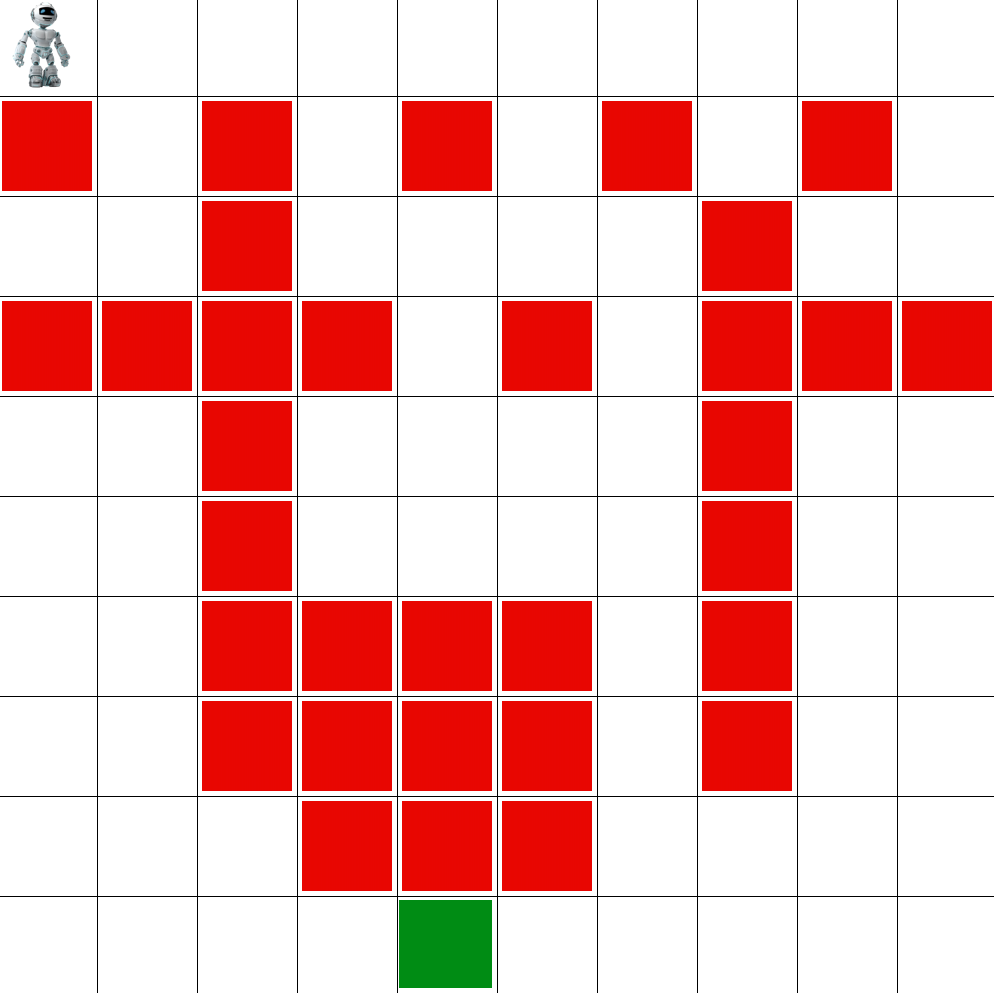
Refer to caption
Figure 6: Illustration of the maze environment.

CartPole:

As mentioned, to translate the image data into states, we used a CNN with: (1) First hidden layer with 646464 filters of 5×5555\times 5 with stride 333 with a ReLU activation, second hidden layer with 646464 filters of 4×4444\times 4 with stride 222 and a ReLU activation, third hidden layer with 646464 filters of 3×3333\times 3 with stride 111 and a ReLU activation. The final hidden layer is “features” we used in an image that is fully connected Flatten units.

Maximum number of steps for the CartPole problem is set to 200200200. We set the ε𝜀\varepsilon-greedy exploration rate to εe=0.5subscript𝜀𝑒0.5\varepsilon_{e}=0.5 for the adaptation phase with decay rate of 0.99990.99990.9999, this value is set to zero in testing phase. The source learned policy is with pole’s length of 0.5m0.5𝑚0.5m and accordingly, using Algorithm 1 in the paper the corresponding successor features are extracted. We used generic Q-learning with replay buffer size 105superscript10510^{5} and Adam optimizer with batch size 646464 to find this optimal policy. The target environment is then modified to incorporate the change of environment. Figure 5 demonstrates the change of dynamics. We used the same structure of feature function in Maze problem for this experiment.

FSF:

This environment (Barreto et al., 2020) is a 10×10101010\times 10 grid with 101010 objects and an agent occupying one cell at each time step. There are 222 types of objects each with a reward associated with it. We randomly initialise those 101010 objects by sampling both their type and position from a uniform distributions over the corresponding sets. Likewise, the initial position of the agent is a uniform sample of all possible positions in the grid. The reward function is defined by the object type that has been picked up by the agent. e.g. Picking up red object is +11+1 reward and picking up blue is 11-1. Agent picks up an object if it occupies that particular cell in which the object exists. If agent picks up an object, another one will be generated randomly (in terms of location and type) in the grid. At each step the agent receives an observation representing the configuration of the environment (Barreto et al., 2020). These are 11×11×(𝔻+1)1111𝔻111\times 11\times(\mathbb{D}+1) tensors that can be seen as 11×11111111\times 11 images with (𝔻+1)𝔻1(\mathbb{D}+1) channels that are used to identify objects and walls (Barreto et al., 2020). The observations are shifted so that the the agent is always at the top-left cell of the grid. Figure 7 shows an example of this environment. The two source policies used in this experiment have 𝐰1=[1,0],𝐰2=[1,0],formulae-sequencesubscript𝐰110subscript𝐰210\mathrm{\bm{w}_{1}=[1,0]},\mathrm{\bm{w}_{2}=[1,0]}, respectively. Intuitively, the reward mappers indicate picking up an object of particular type and ignoring the other type. However, in the target environment, the change of reward function is to pick up the first object type and “avoid” the second one with negative reward - i.e. 𝒘𝒯=[1,1].subscript𝒘𝒯11\bm{w}_{\mathcal{T}}=[1,-1]. For the dissimilarity of dynamics, we added 5%percent55\% noise to the transitions of the agent and also randomly placed a terminal state in the target environment with -1 reward.
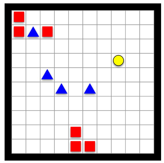
Refer to caption
Figure 7: An example of the environment described in FSF (Barreto et al., 2020).

7.1 Additional Experiments

In this section, we compare our results in navigation problem with generic Q-Learning. We relaxed the assumption adaptation and testing phase and Q-Learning is allowed to use all the observations from the target environment. Figure 8 shows Q-Learning also converges to the same amount of avg. reward, however, since no transfer is involved, it is significantly slower than other baselines. For Q-Learning, we set εe=0.9subscript𝜀𝑒0.9\varepsilon_{e}=0.9 with a decay rate of 0.99990.99990.9999 in 104superscript10410^{4} iterations.

Refer to caption
Figure 8: Performance of Q-Learning in navigation problem.