Optimal ball and horoball packings generated by $3$-dimensional simply truncated Coxeter orthoschemes with parallel faces

Abstract

In this paper we consider the ball and horoball packings belonging to $3$-dimensional Coxeter tilings that are derived by simply truncated orthoschemes with parallel faces.

The goal of this paper to determine the optimal ball and horoball packing arrangements and their densities for all above Coxeter tilings in hyperbolic 3-space $\mathbb{H}^{3}$. The centers of horoballs are required to lie at ideal vertices of the polyhedral cells constituting the tiling, and we allow horoballs of different types at the various vertices.

We prove that the densest packing of the above cases is realized by horoballs related to $\{\infty;3;6;\infty\}$ and $\{\infty;6;3;\infty\}$ tilings with density $\approx 0.8413392$.

1 Introduction, preliminary results

In hyperbolic spaces $\mathbb{H}^{n}$ for $2\leq n\leq 9$, the known densest ball and horoball configurations are derived by Coxeter simplex tilings, therefore it is interesting to determine their optimal horoball packings related to Coxeter tilings. In the former papers, we investigated that Coxeter simplex tilings whose generating simplices do not have parallel faces. Now, we extend our study to the $3$ dimensional Coxeter tilings generated by simple frustum orthoschemes with parallel faces. But first, we summarize the results related to the above topic.

Let $X$ denote a space of constant curvature, either the $n$-dimensional sphere $\mathbb{S}^{n}$, Euclidean space $\mathbb{E}^{n}$, or hyperbolic space $\mathbb{H}^{n}$ with $n\geq 2$. An important question of discrete geometry is to find the highest possible packing density in $X$ by congruent non-overlapping balls of a given radius [1], [10]. The definition of packing density is critical in hyperbolic space as shown by Böröczky [5, 6], for the standard paradoxical construction see [10]. The most widely accepted notion of packing density considers the local densities of balls with respect to their Dirichlet–Voronoi cells (cf. [7] and [18]). In order to study horoball packings in $\overline{\mathbb{H}}^{n}$, we use an extended notion of such local density.

Let $B$ be a horoball of packing $\mathcal{B}$, and $P\in\overline{\mathbb{H}}^{n}$ an arbitrary point. Define $d(P,B)$ to be the shortest distance from point $P$ to the horosphere $S=\partial B$, where $d(P,B)\leq 0$ if $P\in B$. The Dirichlet–Voronoi cell $\mathcal{D}(B,\mathcal{B})$ of horoball $B$ is the convex body

$$\mathcal{D}(B,\mathcal{B})=\{P\in\mathbb{H}^{n}|d(P,B)\leq d(P,B^{\prime}),\leavevmode\nobreak\ \forall B^{\prime}\in\mathcal{B}\}.$$

Both $B$ and $\mathcal{D}$ have infinite volume, so the standard notion of local density is modified. Let $Q\in\partial{\mathbb{H}}^{n}$ denote the ideal center of $B$, and take its boundary $S$ to be the one-point compactification of Euclidean $(n-1)$-space. Let $B_{C}^{n-1}(r)\subset S$ be the Euclidean $(n-1)$-ball with center $C\in S\setminus\{Q\}$. Then $Q$ and $B_{C}^{n-1}(r)$ determine a convex cone $\mathcal{C}^{n}(r)=cone_{Q}\left(B_{C}^{n-1}(r)\right)\in\overline{\mathbb{H}}^{n}$ with apex $Q$ consisting of all hyperbolic geodesics passing through $B_{C}^{n-1}(r)$ with limit point $Q$. The local density $\delta_{n}(B,\mathcal{B})$ of $B$ to $\mathcal{D}$ is defined as

$$\delta_{n}(\mathcal{B},B)=\varlimsup\limits_{r\rightarrow\infty}\frac{vol(B\cap\mathcal{C}^{n}(r))}{vol(\mathcal{D}\cap\mathcal{C}^{n}(r))}.$$

This limit is independent of the choice of center $C$ for $B^{n-1}_{C}(r)$.

In the case of periodic ball or horoball packings, this local density defined above can be extended to the entire hyperbolic space, and is related to the simplicial density function (defined below) that we generalized in [31] and [32]. In this paper, we shall use such definition of packing density (cf. Section 3).

A Coxeter simplex is a top dimensional simplex in $X$ with dihedral angles either integral submultiples of $\pi$ or zero. The group generated by reflections on the sides of a Coxeter simplex is a Coxeter simplex reflection group. Such reflections generate a discrete group of isometries of $X$ with the Coxeter simplex as the fundamental domain; hence the groups give regular tessellations of $X$ if the fundamental simplex is characteristic. The Coxeter groups are finite for $\mathbb{S}^{n}$, and infinite for $\mathbb{E}^{n}$ or $\overline{\mathbb{H}}^{n}$.

There are non-compact Coxeter simplices in $\overline{\mathbb{H}}^{n}$ with ideal vertices in $\partial\mathbb{H}^{n}$, however only for dimensions $2\leq n\leq 9$; furthermore, only a finite number exists in dimensions $n\geq 3$. Johnson et al. [16] found the volumes of all mentioned Coxeter simplices in hyperbolic $n$-space, also see Kellerhals [18]. Such simplices are the most elementary building blocks of hyperbolic manifolds, the volume of which is an important topological invariant.

In $n$-dimensional space $X$ of constant curvature $(n\geq 2)$, define the simplicial density function $d_{n}(r)$ to be the density of $n+1$ mutually tangent balls of radius $r$ in the simplex spanned by their centers. L. Fejes Tóth and H. S. M. Coxeter conjectured that the packing density of balls of radius $r$ in $X$ cannot exceed $d_{n}(r)$. Rogers [29] proved this conjecture in Euclidean space $\mathbb{E}^{n}$. The $2$-dimensional spherical case was settled by L. Fejes Tóth [11], and Böröczky [7], who extend the analogous statement to $n$-dimensional sapces of constant curvature.

In hyperbolic 3-space, the monotonicity of $d_{3}(r)$ was proved by Böröczky and Florian in [8]; in [25] Marshall showed that for sufficiently large $n$, function $d_{n}(r)$ is strictly increasing in variable $r$.

The simplicial packing density upper bound $d_{3}(\infty)=(1+\frac{1}{2^{2}}-\frac{1}{4^{2}}-\frac{1}{5^{2}}+\frac{1}{7^{2}}+\frac{1}{8^{2}}--++\dots)^{-1}=0.85327\dots$ cannot be achieved by packing regular balls, instead it is realized by horoball packings of $\overline{\mathbb{H}}^{3}$, the regular ideal simplex tiles $\overline{\mathbb{H}}^{3}$. More precisely, the centers of horoballs in $\partial\overline{\mathbb{H}}^{3}$ lie at the vertices of the ideal regular Coxeter simplex tiling with Schläfli symbol $\{3,3,6\}$.

In [20] we proved that this optimal horoball packing configuration in $\mathbb{H}^{3}$ is not unique. We gave several more examples of regular horoball packing arrangements based on asymptotic Coxeter tilings using horoballs of different types, that is horoballs that have different relative densities with respect to the fundamental domain, that yield the Böröczky–Florian-type simplicial upper bound [8].

Furthermore, in [31, 32] we found that by allowing horoballs of different types at each vertex of a totally asymptotic simplex and generalizing the simplicial density function to $\overline{\mathbb{H}}^{n}$ for $(n\geq 2)$, the Böröczky-type density upper bound is not valid for the fully asymptotic simplices for $n\geq 4$. For example, in $\overline{\mathbb{H}}^{4}$ the locally optimal simplicial packing density is $0.77038\dots$, higher than the Böröczky-type density upper bound of $d_{4}(\infty)=0.73046\dots$ using horoballs of a single type. However these ball packing configurations are only locally optimal and cannot be extended to the entirety of the ambient space $\overline{\mathbb{H}}^{n}$. In [21] we found seven horoball packings of Coxeter simplex tilings in $\overline{\mathbb{H}}^{4}$ that yield densities of $5\sqrt{2}/\pi^{2}\approx 0.71645$, counterexamples to L. Fejes Tóth’s conjecture of $\frac{5-\sqrt{5}}{4}$ stated in his foundational book Regular Figures [11, p. 323].

In [22], [23] we extend our study of horoball packings to $\overline{\mathbb{H}}^{n}$ ($5\leq n\leq 9$) using our methods that were successfully applied in lower dimensions.

In the previously mentioned papers, we studied the ball and horoball packing related to the Coxeter simplex tilings where the vertices of the simplices are proper points of the hyperbolic space $\mathbb{H}^{n}$ or they are ideal i.e. lying on the sphere $\partial\mathbb{H}^{n}$.

Now, we consider the Coxeter tilings in $3$-dimensional hyperbolic space $\mathbb{H}^{3}$ where the generating orthoscheme is a simply truncated Coxeter orthoscheme. Moreover, we require that the truncated orthoscheme has parallel faces i.e. their dihedral angle is zero.

In $\mathbb{H}^{3}$ the simply truncated orthoscheme tilings (crystallographic Napier cycles of type 2 see [13, 14]) are determined by the following Coxeter-Schläfli graphs:

where $\frac{1}{p}+\frac{1}{q}<\frac{1}{2}$ and $\frac{1}{q}+\frac{1}{r}\geq\frac{1}{2}$, ($3\leq p,q,r\in\mathbb{N}$).

Remark 1.1

The first cases are investigated in papers [38, 39, 40] where from the truncated orthoschemes can be derived prism-like tilings generated hyperball or hyp-hor packings (or coverings) in $\mathbb{H}^{3}$.

In this paper, we concentrate on the second tilings which are given with Schläfli symbol $\{\infty,q,r,\infty\}$. We determine the optimal ball and horoball packings related to the above tilings prove that the densest packing arrangement of the considered tilings is realized at the tilings $\{\infty,3,6,\infty\}$, and $\{\infty;6;3;\infty\}$ by horoballs with density $\approx 0.8413392$. Our results are summarized in Theorems 3.5, 4.2, 4.4 and in Tables 1,3,4.

2 Basic notions

2.1 The projective model of hyperbolic space $\mathbb{H}^{3}$

For the computations, we use the projective model [26] of the hyperbolic space. The model is defined in the $\mathbb{E}^{1,n}$ Lorentz space with signature $(1,n)$, i.e. consider $\mathbf{V}^{n+1}$ real vector space equipped with the bilinear form:

$$\langle\leavevmode\nobreak\ \mathbf{x},\leavevmode\nobreak\ \mathbf{y}\rangle=-x^{0}y^{0}+x^{1}y^{1}+\dots+x^{n}y^{n}.$$

In the vector space, consider the following equivalence relation:

$$\mathbf{x}(x^{0},...,x^{n})\thicksim\mathbf{y}(y^{0},...,y^{n})\Leftrightarrow\exists\leavevmode\nobreak\ c\in\mathbb{R}\backslash\{0\}:\mathbf{y}=c\cdot\mathbf{x}$$

The factorization with $\thicksim$ induces the $\mathcal{P}^{n}(\mathbf{V}^{n+1},\mbox{\boldmath$V$}\!_{n+1})$ $n$-dimensional real projective space. In this space to interpret the points of $\mathbb{H}^{n}$ hyperbolic space, consider the following quadratic form:

$$Q=\{[\mathbf{x}]\in\mathcal{P}^{n}|\langle\leavevmode\nobreak\ \mathbf{x},\leavevmode\nobreak\ \mathbf{x}\rangle=0\}=:\partial\mathbb{H}^{n}$$

The inner points relative to the cone-component determined by $Q$ are the points of $\mathbb{H}^{n}$ (for them $\langle\leavevmode\nobreak\ \mathbf{x},\leavevmode\nobreak\ \mathbf{x}\rangle<0$), the point of $Q=\partial\mathbb{H}^{n}$ are called the points at infinity, and the points lying outside relative to $Q$ are outer points of $\mathbb{H}^{n}$ (for them $\langle\leavevmode\nobreak\ \mathbf{x},\leavevmode\nobreak\ \mathbf{x}\rangle>0$). We can also define a linear polarity between the points and hyperplanes of the space: the polar hyperplane of a point $[\mathbf{x}]\in\mathcal{P}^{n}$ is $Pol(\mathbf{x}):=\{[\mathbf{y}]\in\mathcal{P}^{n}|\langle\leavevmode\nobreak\ \mathbf{x},\leavevmode\nobreak\ \mathbf{y}\rangle=0\}$, and hence $\mathbf{x}\in\mathbf{V}^{n+1}$ is incident with ${\boldsymbol{a}}\in\mbox{\boldmath$V$}\!_{n+1}$ iff $\langle\leavevmode\nobreak\ \mathbf{x},\leavevmode\nobreak\ {\boldsymbol{a}}\rangle=0$. In this projective model, we can define a metric structure related to the above bilinear form, where for the distance of two proper points:

$$\cosh(\frac{d(\mathbf{x},\mathbf{y})}{k})=\frac{-\langle\leavevmode\nobreak\ \mathbf{x},\leavevmode\nobreak\ \mathbf{y}\rangle}{\sqrt{\langle\leavevmode\nobreak\ \mathbf{x},\leavevmode\nobreak\ \mathbf{x}\rangle\langle\leavevmode\nobreak\ \mathbf{y},\leavevmode\nobreak\ \mathbf{y}\rangle}},\leavevmode\nobreak\ (\text{at present}\leavevmode\nobreak\ k=1).$$ (2.1)

This corresponds to the distance formula in the well-known Beltrami-Cayley-Klein model.

2.2 Coxeter orthoschemes and tilings

Definition 2.1

In the $\mathbb{H}^{n}$ $(2\leq n\in\mathbb{N})$ space a complete orthoscheme $\mathcal{O}$ of degree $d$ $(0\leq d\leq 2)$ is a polytope bounded with hyperplanes $H^{0},...,H^{n+d}$, for which $H^{i}\perp H^{j}$, unless $j\neq i-1,i,i+1$.

In the classical ($d=0$) case, let denote the vertex opposite to $H^{i}$ hyperplane with $A_{i}$ ($0\leq i\leq n$), and let denote the dihedral angle of $H^{i}$ and $H^{j}$ planes with $\alpha^{ij}$ (hence $\alpha^{ij}$ if $0\leq i<j-1\leq n$).

In this paper, we deal with orthoschemes of degree $d=1$, they can be described geometrically, as follows. We can give the sequence of the vertices of the orthoschemes $A_{0},...,A_{n}$, where $A_{i}A_{i+1}$ edge is perpendicular to $A_{i+2}A_{i+3}$ edge for all $i\in\{0,...,n-3\}$. Here $A_{0}$ and $A_{n}$ are called the principal vertices of the orthoschemes. In the case $d=1$, one of these principal vertices (e.g. $A_{0}$) is the outer points of the above model, so they are truncated by its polar planes $Pol(A_{0})$ and the orthoscheme is called simply truncated.

In general, the Coxeter orthoschemes were classified by H-C. Im Hof, he proved that they exist in dimension $\leq 9$, and gave a full list of them [13], [14].

Now consider the reflections on the facets of the simly truncated orthoscheme, and denote them with $r_{1},...,r_{n+2}$, hence define the group

$$\mathbf{G}=\langle r_{1},...,r_{n+2}|(r_{i}r_{j})^{m_{ij}}=1\rangle,$$

where $\alpha^{ij}=\frac{\pi}{m_{ij}}$, so $m_{ii}=1$, and if $m_{ij}=\infty$ (i.e. $H^{i}$ and $H^{j}$ are parallel), than to the $r_{i},r_{j}$ pair belongs no relation. Suppose that $2\leq m_{ij}\in\{\mathbb{N}\cup\infty\}$ if $i\neq j$. The Coxeter group $\mathbf{G}$ acts on hyperbolic space $\overline{\mathbb{H}}^{n}$ properly discontinously, thus the images of the orthoscheme under this action provide a $\mathcal{T}$ tiling of $\overline{\mathbb{H}}^{n}$ (i.e. the images of the orthoscheme fills $\overline{\mathbb{H}}^{n}$ without overlap).

For the complete Coxeter orthoschemes $\mathcal{S}\subset\mathbb{H}^{n}$, we adopt the usual conventions and sometimes even use them in the Coxeter case: if two nodes are related by the weight $\cos{\frac{\pi}{m_{ij}}}$ then they are joined by a ($m_{ij}-2$)-fold line for $m_{ij}=3,\leavevmode\nobreak\ 4$ and by a single line marked by $m_{ij}$ for $m_{ij}\geq 5$. In the hyperbolic case if two bounding hyperplanes of $S$ are parallel, then the corresponding nodes are joined by a line marked $\infty$. If they are divergent then their nodes are joined by a dotted line.

In the following we concentrate only on dimension $3$, $\overline{\mathbb{H}}^{3}$. For every considered tiling there is a corresponding symmetric $4\times 4$ matrix $(b^{ij})$ where $b^{ii}=1$ and, for $i\neq j\in\{0,1,2,3\}$, $b^{ij}$ equals to $-\cos{\alpha_{ij}}$ with all dihedral angles $\alpha_{ij}$ between the faces $u_{i}$,$u_{j}$ of $\mathcal{S}$.

The matrix $(b^{ij})$ in formula (2.2) is the so called Coxeter-Schläfli matrix with parameters $(p;q;r)$, i.e. $\alpha_{01}=\frac{\pi}{p}$, $\alpha_{12}=\frac{\pi}{q}$, $\alpha_{23}=\frac{\pi}{r}$. Now only $3\leq p,q,r\in\mathbb{N}$ come into account (see [13, 14]).

$$(b^{ij})=\langle\mbox{\boldmath$b^{i}$},\mbox{\boldmath$b^{j}$}\rangle:=\begin{pmatrix}1&-\cos{(\frac{\pi}{p})}&0&0\\ -\cos{(\frac{\pi}{p})}&1&-\cos{(\frac{\pi}{q})}&0\\ 0&-\cos{(\frac{\pi}{q})}&1&-\cos{(\frac{\pi}{r})}\\ 0&0&-\cos{(\frac{\pi}{r})}&1\end{pmatrix}.$$ (2.2)

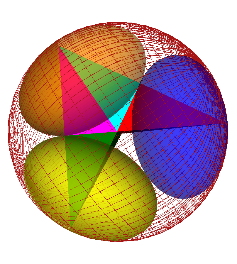
Figure 5: Horospheres packing configuration related to the truncated orthoscheme $\{\infty,3,3,\infty\}$

This $3$-dimensional complete (truncated or frustum) orthoscheme $\mathcal{S}=\mathcal{S}(p;q;r)$ tilings are described in Fig. 5, 6, 7 and they are characterised by their symmetric Coxeter-Schläfli matrices $(b^{ij})$ (see formula (2.2)), furthermore by their inverse matrices $(h_{ij})$ in formula (2.3).

$$\begin{gathered}(h_{ij})=(b^{ij})^{-1}=\langle\mathbf{a}_{i},\mathbf{a}_{j}\rangle:=\\ =\frac{1}{B}\begin{pmatrix}\sin^{2}{(\frac{\pi}{r})}-\cos^{2}{(\frac{\pi}{q})}&\cos{(\frac{\pi}{p})}\sin^{2}{(\frac{\pi}{r})}&\cos{(\frac{\pi}{p})}\cos{(\frac{\pi}{q})}&\cos{(\frac{\pi}{p})}\cos{(\frac{\pi}{q})}\cos{(\frac{\pi}{r})}\\ \cos{(\frac{\pi}{p})}\sin^{2}{(\frac{\pi}{r})}&\sin^{2}{(\frac{\pi}{r})}&\cos{(\frac{\pi}{q})}&\cos{(\frac{\pi}{r})}\cos{(\frac{\pi}{q})}\\ \cos{(\frac{\pi}{p})}\cos{(\frac{\pi}{q})}&\cos{(\frac{\pi}{q})}&\sin^{2}{(\frac{\pi}{p})}&\cos{(\frac{\pi}{r})}\sin^{2}{(\frac{\pi}{p})}\\ \cos{(\frac{\pi}{p})}\cos{(\frac{\pi}{q})}\cos{(\frac{\pi}{r})}&\cos{(\frac{\pi}{r})}\cos{(\frac{\pi}{q})}&\cos{(\frac{\pi}{r})}\sin^{2}{(\frac{\pi}{p})}&\sin^{2}{(\frac{\pi}{p})}-\cos^{2}{(\frac{\pi}{q})}\end{pmatrix},\end{gathered}$$ (2.3)

where

$$B=\det(b^{ij})=\sin^{2}{\left(\frac{\pi}{p}\right)}\sin^{2}{\left(\frac{\pi}{r}\right)}-\cos^{2}{\left(\frac{\pi}{q}\right)}<0,\ \ \text{i.e.}\ \sin{\left(\frac{\pi}{p}\right)}\sin{\left(\frac{\pi}{r}\right)}-\cos{\left(\frac{\pi}{q}\right)}<0.$$

In this work, our aim is to study the Coxeter tilings generated by simply truncated orthoschemes with Coxeter-Schläfli graph $\{\infty;q;r;\infty\}$. In these cases, the truncated orthoscheme is a $3$-dimensional hyperbolic polyhedron bounded by $5$ faces $u_{i}$ ($i=0,\dots 4$) that are determined by its form $\boldsymbol{u}_{i}$. If the parameters $p,q,r$ satisfy $\frac{1}{p}+\frac{1}{q}<\frac{1}{2}$ and $\frac{1}{q}+\frac{1}{r}\geq\frac{1}{2}$, ($3\leq p,q,r\in\mathbb{N})$ then the corresponding Coxeter-Schläfli matrix is

$$(B^{ij})=\begin{pmatrix}1&-\cos{(\frac{\pi}{p})}&0&0&0\\ -\cos{(\frac{\pi}{p})}&1&-\cos{(\frac{\pi}{q})}&0&0\\ 0&-\cos{(\frac{\pi}{q})}&1&-\cos{(\frac{\pi}{r})}&0\\ 0&0&-\cos{(\frac{\pi}{r})}&1&c_{4}\\ 0&0&0&c_{4}&1\end{pmatrix},$$ (2.4)

where the constant $c_{4}$ can be uniquely determined in the arrangement of Napier cycles [13]

$$c_{4}=-\sqrt{\frac{1+\cos^{2}(\frac{\pi}{p})\cos^{2}(\frac{\pi}{r})-\cos^{2}(\frac{\pi}{p})-\cos^{2}(\frac{\pi}{q})-\cos^{2}(\frac{\pi}{r})}{1-\cos^{2}(\frac{\pi}{p})-\cos^{2}(\frac{\pi}{q})}}.$$

In our case, there are two parallel faces (hyperplanes) that meet at the ideal point. That means the dihedral angle between these two hyperplanes are equal to zero. Therefore, we assume that these two hyperplane are $u_{0}$ and $u_{1}$, in such their dihedral angle is $w_{0}=\frac{\pi}{p}=0$. The corresponding Coxeter-Schläfli matrix $(B^{ij})$ can be described in the following form:

$$(B^{ij})=\begin{pmatrix}1&-1&0&0&0\\ -1&1&-\cos{(\frac{\pi}{q})}&0&0\\ 0&-\cos{(\frac{\pi}{q})}&1&-\cos{(\frac{\pi}{r})}&0\\ 0&0&-\cos{(\frac{\pi}{r})}&1&-1\\ 0&0&0&-1&1\end{pmatrix}$$ (2.5)

The matrix $(B^{ij})$ is a singular matrix whose non-singular $4\times 4$ principal submatrix is $(b^{ij})$.

The volume of a simply truncated Coxeter orthoscheme with outer vertices $A_{0}$ can be determined by the following theorem of R. Kellerhals [18, 19].

Theorem 2.1

The volume of a three-dimensional hyperbolic complete orthoscheme (except Lambert cube cases) $\mathcal{S}$ is expressed with the essential angles $\alpha^{01},\alpha^{12},\alpha^{23},\\ (0\leq\alpha^{ij}\leq\frac{\pi}{2})$ in the following form:

$$Vol_{3}(\mathcal{S})=\frac{1}{4}\{\mathcal{L}(\alpha^{01}+\theta)-\mathcal{L}(\alpha^{01}-\theta)+\mathcal{L}(\frac{\pi}{2}+\alpha^{12}-\theta)+$$

$$+\mathcal{L}(\frac{\pi}{2}-\alpha^{12}-\theta)+\mathcal{L}(\alpha^{23}+\theta)-\mathcal{L}(\alpha^{23}-\theta)+2\mathcal{L}(\frac{\pi}{2}-\theta)\},$$

where $\theta\in[0,\frac{\pi}{2})$ is defined by the following formula:

$$\tan(\theta)=\frac{\sqrt{\cos^{2}{\alpha^{12}}-\sin^{2}{\alpha^{01}}\sin^{2}{\alpha^{23}}}}{\cos{\alpha^{01}}\cos{\alpha^{23}}}$$

and where $\mathcal{L}(x):=-\int\limits_{0}^{x}\log|{2\sin{t}}|dt$  denotes the Lobachevsky function.

In this paper, we consider that Coxeter orthoscheme tilings which are given with Schläfli symbol $\{\infty;q;r;\infty\}$ ($\frac{1}{q}+\frac{1}{r}\geq\frac{1}{2}$, $3\leq p,q,r\in\mathbb{N}$) and determine the optimal ball and horoball packings related to the above tilings. The possible parameters are the following:

$$(q,r)=(3,4),(3,5),(3,6),(4,3),(4,4),(4,5),(5,3),(6,3).$$ (2.6)

3 Optimal ball packings

3.1 Inradii of truncated orthoschemes

In determining the radius entered, we must distinguish two cases. The first type includes cases where the inscribed ball of the complete orthoscheme is the same as the inscribed ball of the truncated orthoscheme, and the second case where it is not true.

3.1.1 Type 1

In [15] M. Jacquemet determined the inradii of truncated simplices in $n$-dimensi-onal hyperbolic spaces if their inballs do not have common inner points with the corresponding truncating hyperplanes. We first recall some of the statements from that mentioned paper that we will apply to our calculations.

We use the former section introduced denotation: let $\mathcal{S}$ a complete orthoscheme and $\hat{\mathcal{S}}$ be the considered truncated orthoscheme. The corresponding Coxeter-Schläfli matrix is denoted by $(B^{ij})$ whose principal submatrix $(b^{ij})$.

Lemma 3.1

A truncated hyperbolic simplex $\hat{\mathcal{S}}$ with Coxeter-Schläfli principal submatrix $(b^{ij})$ has inball, (imbedded ball of maximal finite radius) in $\mathbb{H}^{n}$ if only if $\sum_{i,j=1}^{n+1}cof_{ij}({b^{ij}})>0$.

We can rewrite this conditions using $h_{ij}$ (the inverse matrix of $(b^{ij}))$.

$$\sum_{i,j=1}^{n+1}det(b^{ij})(h_{ij})>0$$ (3.1)

Lemma 3.2

Let $(b^{ij})$ be the Coxeter-Schläfli matrix of complete orthoscheme ${\mathcal{S}}$ with inball ${\mathcal{B}}\subset\mathbb{H}^{n}$. Then, the inradius ${r}=r({\mathcal{B}})$ is given by

$${r}=\sinh^{-1}{\sqrt{-\frac{1}{\sum_{i,j=1}^{n+1}h_{ij}}}}.$$ (3.2)

In our case, the orthoscheme is truncated by a polar hyperplane of the vertex which lie outer of the Beltrami-Cayley-Klein model, it is called ultra ideal vertex. Therefore, we need to study whether the inradius of the above orthoscheme and the inradius of the truncated orthoscheme are equal to each other.

Lemma 3.3 ([15])

Let ${\mathcal{S}}$ be an $n$-dimensional simplex with $k\leq n$ vertices are ultra ideal, with Coxeter-Schläfli matrix $(b^{ij})$, such that ${\mathcal{S}}$ has an inball ${B}\subset\mathbb{H}^{n}$ of radius ${r}$. Denote by $\hat{\mathcal{S}}\subset\bar{\mathcal{H}^{n}}$ its associated hyperbolic $k$-truncated simplex with respect to the ultra-ideal vertices $v_{1},\cdots,v_{k}$, $1\leq k$. Let $\hat{r}$ be the inradius of inball of $\hat{\mathcal{S}}$. Then, $r=\hat{r}$ if and only if

$$\frac{\sum_{j=1}^{n+1}cof_{ij}{(b^{ij})}}{det({b^{ij}})cof_{ii}{(b^{ij})}}\geq 1\leavevmode\nobreak\ \leavevmode\nobreak\ \leavevmode\nobreak\ \text{for all}\leavevmode\nobreak\ i=1,\cdots,k.$$ (3.3)

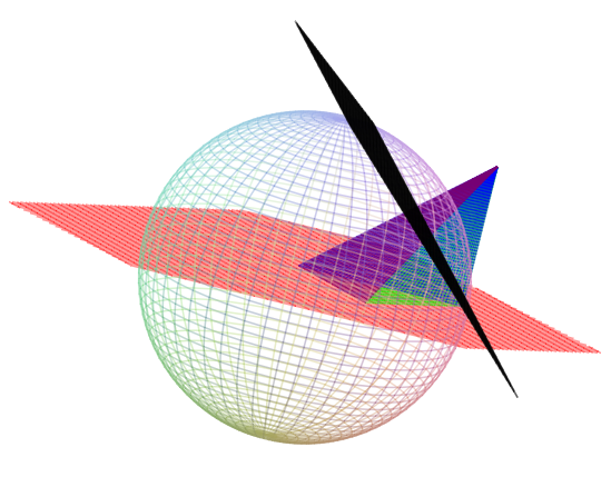
Figure 1: The truncated orthoscheme: $(q,r)=(3,4)$

Figure 2: The structure of truncated orthoscheme with inball and its centre

We apply the above existence conditions for the considered tilings and obtain, ${\det}{(b^{ij})}=-\cos^{2}{\left(\frac{\pi}{q}\right)}$. To confirm the existence of inball in the complete orthoscheme $\mathcal{S}$ we need to clarify whether the value $\sum_{i,j=1}^{n+1}det(b^{ij})h_{ij}$ is a positive number. By the direct computations, we have the following expression

$$\sum_{i,j=1}^{n+1}det(b^{ij})h_{ij}=\left(\frac{4+2\cos^{2}\left(\frac{\pi}{q}\right)+4\cos\left(\frac{\pi}{q}\right)\cos\left(\frac{\pi}{r}\right)-4\cos^{2}\left(\frac{\pi}{r}\right)}{\cos^{2}\left(\frac{\pi}{q}\right)}\right)\cos^{2}\left(\frac{\pi}{q}\right).$$ (3.4)

One could see that in the expression above,

$$\begin{gathered}4+2\cos^{2}\left(\frac{\pi}{q}\right)+4\cos\left(\frac{\pi}{q}\right)\cos\left(\frac{\pi}{r}\right)-4\cos^{2}\left(\frac{\pi}{r}\right)>\\ >4-4\cos^{2}\left(\frac{\pi}{r}\right)>0.\end{gathered}$$ (3.5)

Therefore $\sum_{i,j=1}^{n+1}det(b^{ij})h_{ij}>0$ for all $(q,r)$ in our cases.

Then, we have to determine for which parameters are the inradius $r$ of complete orthoscheme $\mathcal{S}$ equal to the inradius $\hat{r}$ of the truncated orthoscheme $\hat{\mathcal{S}}$.

In our case there is only one ultra ideal vertex therefore, applying the formula (3.3) we get the following inequalities:

$$\begin{gathered}-\frac{\left(1-\frac{2\cos{\left(\frac{\pi}{r}\right)}}{\cos{\left(\frac{\pi}{q}\right)}}\right)\cos^{2}{\left(\frac{\pi}{q}\right)}}{\sqrt{\cos^{4}{\left(\frac{\pi}{q}\right)}}}\geq 1\Leftrightarrow\frac{\cos{\left(\frac{\pi}{r}\right)}}{\cos{\left(\frac{\pi}{q}\right)}}\geq 1.\end{gathered}$$ (3.6)

That inequality could only be satisfied by the parameter tuples of $(q,r)=$ $(3,3)$, $(3,4)$, $(3,5)$, $(3,6)$, $(4,4)$.
Therefore, in these cases the radii of optimal inballs can be determined by formula (3.2).

3.2 Type 2

We consider the case where the inradius of the complete orthoschemes and the truncated orthoschemes are not the same, i.e when the Lemma 3.3 does not hold. This situation happens on the tuple parameters $(4,3),(5,3),(6,3)$. In these cases, the constructed inball intersect the truncated face:

$$r=d(\boldsymbol{c},\boldsymbol{u}_{0})=d(\boldsymbol{c},\boldsymbol{u}_{1})=d(\boldsymbol{c},\boldsymbol{u}_{2})=d(\boldsymbol{c},\boldsymbol{u}_{3})>d(\boldsymbol{c},\boldsymbol{u}_{4}),$$

where $\boldsymbol{c}$ is the insphere center of the complete orthoscheme $\mathcal{S}(q,r)$. Therefore, the problem is that the constructed inball intersects the hyperplane $\boldsymbol{u}_{4}$.

Instead of using the results of [15], we apply the classical way to determine the incenter and its radius in the mentioned cases. Basically, to find the center of optimal inball we determine the hyperplane bisectors of faces of truncated orthoscheme $\hat{\mathcal{S}}(q,r)$. The inball of maximal radius has to touch at least four faces of $\hat{\mathcal{S}}(q,r)$ and one of them must be the face determined by form $[\boldsymbol{u}_{4}]$.

Therefore, we have $4$ analogues cases that provide the candidates for the optimal incenter. We have to determine these centers and we need to select the center with the maximum radius. This optimal ball is denoted by $\mathcal{B}(q,r)$.

3.3 Densest ball packing configurations

The volume of the truncated orthoscheme $\hat{\mathcal{S}}(q,r)$ is denoted by $Vol(\hat{\mathcal{S}}(q,r))$ where $(q,r)=$ $(3,3)$, $(3,4)$, $(3,5)$, $(3,6)$, $(4,4)$, $(4,3)$, $(5,3)$, $(6,3)$. We introduce the local density function $\delta_{opt}(\hat{\mathcal{S}(q,r)})$ related to orthoscheme $\hat{\mathcal{S}(q,r)}$ generated tiling:

Definition 3.4

The local density function $\delta_{opt}(\hat{\mathcal{S}}(q,r))$ related to tiling $\mathcal{T}(q,r)$ generaded by truncated orthoscheme $\hat{\mathcal{S}}(q,r)$:

$$\delta_{opt}(\hat{\mathcal{S}}(q,r)):=\frac{Vol(\mathcal{B}(q,r))}{Vol(\hat{\mathcal{S}}(q,r))}.$$

We obtain the volumes of the $Vol(\mathcal{B}(q,r))$ balls by the classical formula of J. Bolyai $Vol(\mathcal{B}(q,r))=\pi k^{3}\left(\sinh{\left(\frac{2r}{k}\right)}-\frac{2r}{k}\right)$, where at present $k=1$ and the volumes of truncated simplices $\hat{\mathcal{S}}(q,r)$ can be calculated by Theorem 2.1. Using the formulas of the previous subsection we summarize our results in the following table:

Table 1.

$(q,r)$	Inradius $\hat{r}$	$Vol(\mathcal{B}(q,r))$	$Vol(\hat{\mathcal{S}}(p,q))$	$\delta_{opt}(\hat{\mathcal{S}}(q,r))$
$(3,3)$	0.2116177	0.0400529	0.1526609	0.2623649
$(3,4)$	0.2236802	0.0473496	0.2509603	0.1886735
$(3,5)$	0.2335727	0.0539625	0.3323272	0.1623776
$(3,6)$	0.2407179	0.0591079	0.4228923	0.1397706
$(4,3)$	0.2396177	0.0582950	0.2509603	0.2322876
$(4,4)$	0.2888593	0.1026579	0.4579828	0.2241524
$(5,3)$	0.2562904	0.0714478	0.3323273	0.2149924
$(6,3)$	0.2431555	0.0609361	0.4228923	0.1440937

Finally, we obtain the following

Theorem 3.5

In hyperbolic space $\mathbb{H}^{3}$, between congruent ball packings of classical balls, generated by simply truncated Coxeter orthoschemes with parallel faces, the $\mathcal{B}{(3,3)}$ ball configuration provides the densest packing with density $\approx 0.2623649$.

4 Horoball packings

The aim of this section is to determine the optimal horoball packing densities for Coxeter tilings which are given by Schläfli symbol $\{\infty,q,r,\infty\}$ in 3-dimensional hyperbolic space $\mathbb{H}^{3}$ and have at least one vertex at the infinity $\partial\mathbb{H}^{3}$ $(q,r)=$ $(3,3)$, $(3,4)$, $(3,5)$, $(3,6)$, $(4,4)$, $(4,3)$, $(5,3)$, $(6,3)$ their truncated orthoschemes (fundamental domains of of the corresponding Coxeter group $\Gamma(q,r)$). The volume of the truncated orthoscheme $\hat{\mathcal{S}}(q,r)$ is denoted, similarly to the former subsection, by $Vol(\hat{\mathcal{S}}(q,r))$. Moreover, $\mathcal{T}(q,r)$ denotes the corresponding hyperbolic truncated orthoscheme tiling. In cases $(q,r)=(3,6),(4,4),(6,3)$ the fundamental polyhedron has two vertices lying on the absolute $\partial\mathbb{H}^{3}$.

An approach to describing Coxeter tilings involves analysis of their symmetry groups. If $\mathcal{T}(q,r)$ is a Coxeter orthoscheme tiling, then any rigid motion moving one cell into another maps the entire tiling onto itself. Any orthoscheme cell of $\mathcal{T}(q,r)$ can act as the fundamental domain $\hat{\mathcal{S}}(q,r)$ of $\Gamma(q,r)$ generated by reflections on its $2$-dimensional faces.

We define the density of a horoball packing $\mathcal{B}(q,r)$ related to Coxeter orthoscheme tiling $\mathcal{T}(q,r)$ as

$$\delta(\mathcal{B}({q,r}))=\frac{\sum_{i=1}^{k}Vol(\mathcal{B}_{i}\cap\hat{\mathcal{S}}(q,r))}{Vol(\hat{\mathcal{S}}(q,r))}$$ (4.1)

where $\hat{\mathcal{S}}(q,r)$ denotes the fundamental domain orthoscheme of the tiling $\mathcal{T}(q,r)$, $k\in\{1,2\}$ is the number of ideal vertices of $\hat{\mathcal{S}}(q,r)$, and $\mathcal{B}_{i}$ are the horoballs centered at the ideal vertices. We allow horoballs of different types at the ideal vertices of the tiling. A horoball type is allowed if it gives a packing, i.e. no two horoballs have an interior point in common. In addition, we require that no horoball may extend beyond the facet opposite the vertex where it is centered in order that the packing preserves the Coxeter symmetry group of the tiling. If these conditions are satisfied we can use the corresponding Coxeter group $\Gamma(q,r)$ associated to a tiling to extend the packing density from the fundamental domain simplex to all of $\mathbb{H}^{3}$. We denote the optimal horoball packing density

$$\delta_{opt}(\mathcal{B}(q,r))=\sup\limits_{\mathcal{B}(q,r)\text{\leavevmode\nobreak\ packing}}\delta(\mathcal{B}(q,r)).$$ (4.2)

4.0.1 Equations of the horospheres

A horoshere in the hyperbolic geometry is the surface orthogonal to the set of parallel lines, passing through the same point on the absolute quadratic surface $\partial\mathbb{H}^{n}$ (at present $n=3$) (simply absolute) of the hyperbolic space.

We represent hyperbolic space $\mathbb{H}^{3}$ in the Beltrami-Cayley-Klein ball model. We introduce a projective coordinate system using vector basis $\boldsymbol{b}_{i}\ (i=0,1,2,3)$ for $\mathcal{P}^{3}$ where the coordinates of center of the model is $C=(1,0,0,0)$. We pick an arbitrary point at infinity to be $A_{3}=(1,0,0,1)$.

As it is known, the equation of a horosphere with center $A_{3}=(1,0,0,1)$ through point $S=(1,0,0,s)$ is

$$\text{If $s\neq 1$, then}\ \ \ \frac{{(s-1)}^{2}}{1-s^{2}}(-x^{0}x^{0}+x^{1}x^{1}+x^{2}x^{2}+x^{3}x^{3})+{(x^{0}-x^{3})}^{2}=0\Leftrightarrow$$

$$\Leftrightarrow(s-1)(-x^{0}x^{0}+x^{1}x^{1}+x^{2}x^{2}+x^{3}x^{3})-(1+s){(x^{0}-x^{3})}^{2}=0$$

Therefore, we obtain the following equation for the horosphere in Beltrami-Cayley-Klein model related to our Cartesian coordinate system: ($x:=\frac{x^{1}}{x^{0}},\leavevmode\nobreak\ y:=\frac{x^{2}}{x^{0}},\leavevmode\nobreak\ z:=\frac{x^{3}}{x^{0}}$)

$$\frac{2(x^{2}+y^{2})}{1-s}+\frac{4(z-\frac{s+1}{2})^{2}}{{(1-s)}^{2}}=1$$ (4.3)

4.0.2 Volumes of horoball sectors

The length $L(x)$ of a horospheric arc of a chord segment $x$ is determined by the classical formula due to J. Bolyai:

$$L(x)=2\cdot k\sinh{\frac{x}{2k}}\ (\text{at present}\ k=1).$$ (4.4)

The intrinsic geometry of the horosphere is Euclidean, therefore, the area $\mathrm{Area}(A)$ of a horospherical triangle $A$ is computed by the formula of Heron or by Cayley-Menger determinant. The volume of the horoball pieces can be calculated using another formula by J. Bolyai. If the area of a domain on the horoshere is $\mathrm{Area}(A)$, then the volume determined by $A$ and the aggregate of axes drawn from $A$ is equal to

$$V=\frac{1}{2}k\cdot\mathrm{Area}(A)\ \ (\text{at present}\ k=1).$$ (4.5)

4.1 Horoball packings with one horoball

We compute optimal horoball packing density for the Coxeter simplex tiling in case $(q,r)=(3,3)$. The other cases are obtained by using the same method.

Proposition 4.1

The optimal horoball packing density for Coxeter orthoscheme tiling of Schläfli symbol $\{\infty,3,3,\infty\}$ is $\delta_{opt}(\mathcal{B}(3,3))\approx 0.8188080$.

Proof: For the fundamental polyhedron (truncated orthoscheme) $\hat{\mathcal{S}}(3,3))$ of the Coxeter tiling $\mathcal{T}(3,3)$ we fix coordinates for the vertices $A_{0},A_{1},A_{2},A_{4},A_{5}$ (see Fig. 3) to satisfy the angle requirements. The faces of $\hat{\mathcal{S}}(3,3))$ are given by their forms $[\mbox{\boldmath$u$}_{i}]$ $(i=0,1,2,3,4\})$ where $[\mbox{\boldmath$u$}_{4}]$ is the polar plane of outer point $A_{3}$ (see Fig. 3) and the other planes corresponding to the opposite vertex $A_{i}$ $(i=0,1,2,3)$ related to complete orthoscheme ${\mathcal{S}}(3,3))$.

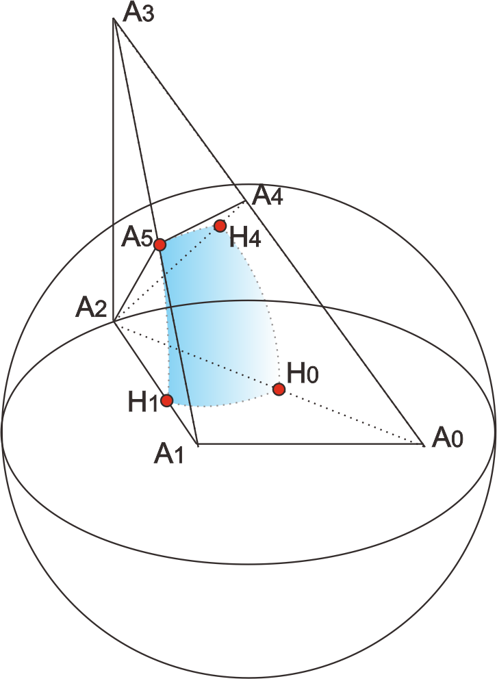
Figure 3: Optimal packing with one horoball type

To maximize the packing density, we determine the maximal horoball type $\mathcal{B}_{2}(s)$ centered at ideal vertex $A_{2}$ that fits into the fundamental domain $\hat{\mathcal{S}}(3,3))$. We find the horoball type parameter $s$ corresponding to the radius of the horoball when the horoball $\mathcal{B}_{2}(s)$ is tangent to the hyperface plane $[\mbox{\boldmath$u$}_{2}]$ bounding the fundamental polyhedron opposite of $A_{2}$. The perpendicular foot $F_{2}[\mbox{\boldmath$f$}_{2}]=A_{5}[\mathbf{a}_{5}]$ of vertex $A_{2}$ on plane $[\mbox{\boldmath$u$}_{2}]$,

$$\mathbf{a}_{5}=\mathbf{a}_{2}-\frac{\langle\mathbf{a}_{2},\mathbf{u}_{2}\rangle}{\langle\mathbf{u}_{2},\mathbf{u}_{2}\rangle}\mathbf{u}_{2}\approx\left(1,\leavevmode\nobreak\ -0.074,\leavevmode\nobreak\ -0.430,0.257\right),$$ (4.6)

is the point of tangency of the maximal horoball and face $[\mbox{\boldmath$u$}_{2}]$ of the orthoscheme cell.

Plugging in $F_{2}=H_{5}$ and solving equation (4.3) we get the parameter of the optimal horoball type. The equation of horosphere $\mathcal{B}_{2}$ centered at $A_{2}$ passing through $F_{2}=A_{5}$ can be determined by formulas (4.3) and (4.5).

The intersections $H_{i}[\mathbf{h}_{i}]$ of the horosphere $\mathcal{B}_{2}$ and the orthoscheme edges are found by parameterizing the simplex edges as $\mathbf{h}_{i}(\lambda)=\lambda\mathbf{a}_{2}+\mathbf{a}_{i}$ $(i=1,2,3,4)$, and computing their intersections with the horopshere (see Fig. 3).

The volume of the horospherical quadrilateral $A=H_{0}H_{1}H_{4}H_{5}$ determines the volume of the horoball piece by equation (4.5). In order to determine the data of the horospheric quadrilateral we compute the hyperbolic distances $l_{ij}$ by the formula (2.1) $l_{ij}=d(H_{i},H_{j})$. Moreover, the horospherical distances $L_{ij}$ can be calculated by the formula (4.4).

In the following table, we summarize the corresponding hyperbolic distances, horospherical distances:

Table 2.

Edge $H_{i}H_{j}$	Hyperbolic distance $l_{ij}$	Horospherical distance $L_{ij}$
$H_{0}H_{1}$	0.4949329	0.5000000
$H_{1}H_{4}$	0.4949329	0.5000000
$H_{0}H_{4}$	0.6931471	0.7071067
$H_{4}H_{5}$	0.4949329	0.5000000
$H_{0}H_{5}$	0.4949329	0.5000000

To determine the area of quadrilateral $A=H_{0}H_{1}H_{4}H_{5}$, divide it into two horospheric triangles using a horospheric diagonal curve. The intrinsic geometry of the horosphere is Euclidean so we can use it to find the area $\mathrm{Area}(A)$ of $A$ the Cayley-Menger determinant:

$$\begin{gathered}\mathrm{Area}(H_{0}H_{1}H_{4})=\left(\frac{(-1)^{3}}{(2!)^{2}2^{2}}\begin{vmatrix}0&1&1&1\\ 1&0&L_{0,1}^{2}&L_{04}^{2}\\ 1&L_{10}^{2}&0&L_{14}^{2}\\ 1&L_{40}^{2}&L_{41}^{2}&0\end{vmatrix}\right)^{\frac{1}{2}}\approx 0.1250000,\\ \mathrm{Area}(H_{0}H_{4}H_{5})=\left(\frac{(-1)^{3}}{(2!)^{2}2^{2}}\begin{vmatrix}0&1&1&1\\ 1&0&L_{04}^{2}&L_{05}^{2}\\ 1&L_{40}^{2}&0&L_{45}^{2}\\ 1&L_{50}^{2}&L_{54}^{2}&0\end{vmatrix}\right)^{\frac{1}{2}}\approx 0.1250000,\\ \Rightarrow\mathrm{Area}(A)=\mathrm{Area}(H_{0}H_{1}H_{4})+\mathrm{Area}(H_{0}H_{4}H_{5})\approx 0.2500000.\end{gathered}$$ (4.7)

The volume of the optimal horoball piece contained in the fundamental truncated orthoscheme $\hat{\mathcal{S}}(3,3))$ is

$$Vol(\mathcal{B}_{2}\cap\hat{\mathcal{S}}(3,3)))=\frac{1}{2}\mathrm{Area}(A)\approx 0.1250000.$$ (4.8)

Hence, the optimal horoball packing density of the Coxeter orthoscheme tiling $\mathcal{T}(3,3)$ becomes

$$\delta_{opt}(\mathcal{B}({3,3}))=\frac{Vol(\mathcal{B}_{2}\cap\hat{\mathcal{S}}(3,3))}{Vol(\hat{\mathcal{S}}(q,r))}\approx 0.8188080.$$ (4.9)

The same method is used to find the optimal packing density of the remaining Coxeter truncated orthoscheme tilings. In cases if the truncated orthoscheme has two ideal vertices (vertices lying at the infinity) then the optimal horoball packing configurations with one horoball are interesting, too. Therefore, we determine both optimal packing arrangements and their densities.

The results of the computations are summarized in Table 3 (see Fig. 4, 5).

Table 3.

Schläfli symbol	$Vol(\mathcal{B}_{i}\cap\hat{\mathcal{S}}(q,r))$	$Vol(\hat{\mathcal{S}}(q,r))$	$\delta_{opt}(\mathcal{B}({q,r}))$.
$(\infty,3,3,\infty),\leavevmode\nobreak\ i=2$	0.1250000	0.1526609	0.8188080
$(\infty,3,4,\infty),\leavevmode\nobreak\ i=2$	0.1767766	0.2509603	0.7044011
$(\infty,3,5,\infty),\leavevmode\nobreak\ i=2$	0.2022543	0.3323272	0.6085997
$(\infty,3,6,\infty),\leavevmode\nobreak\ i=2$	0.2165064	0.4228923	0.5048035
$(\infty,3,6,\infty),\leavevmode\nobreak\ i=0$	0.1443376	0.4228923	0.3365357
$(\infty,4,3,\infty),\leavevmode\nobreak\ i=2$	0.1767766	0.2509603	0.7044011
$(\infty,4,4,\infty),\leavevmode\nobreak\ i=2$	0.2500000	0.4579828	0.5458720
$(\infty,4,4,\infty),\leavevmode\nobreak\ i=0$	0.2500000	0.4579828	0.5458720
$(\infty,5,3,\infty),\leavevmode\nobreak\ i=2$	0.2022543	0.3323272	0.6085997
$(\infty,6,3,\infty),\leavevmode\nobreak\ i=2$	0.2165064	0.4288923	0.5048035
$(\infty,6,3,\infty),\leavevmode\nobreak\ i=0$	0.1443376	0.4288923	0.3365357

We summarize the results of this section in the following

Theorem 4.2

In hyperbolic space $\mathbb{H}^{3}$, between the congruent horoball packings of one horoball, generated by simply truncated Coxeter orthoschemes with parallel faces, the $\mathcal{B}{(3,3)}$ horoball configuration provides the densest packing with density $\approx 0.8188080$.

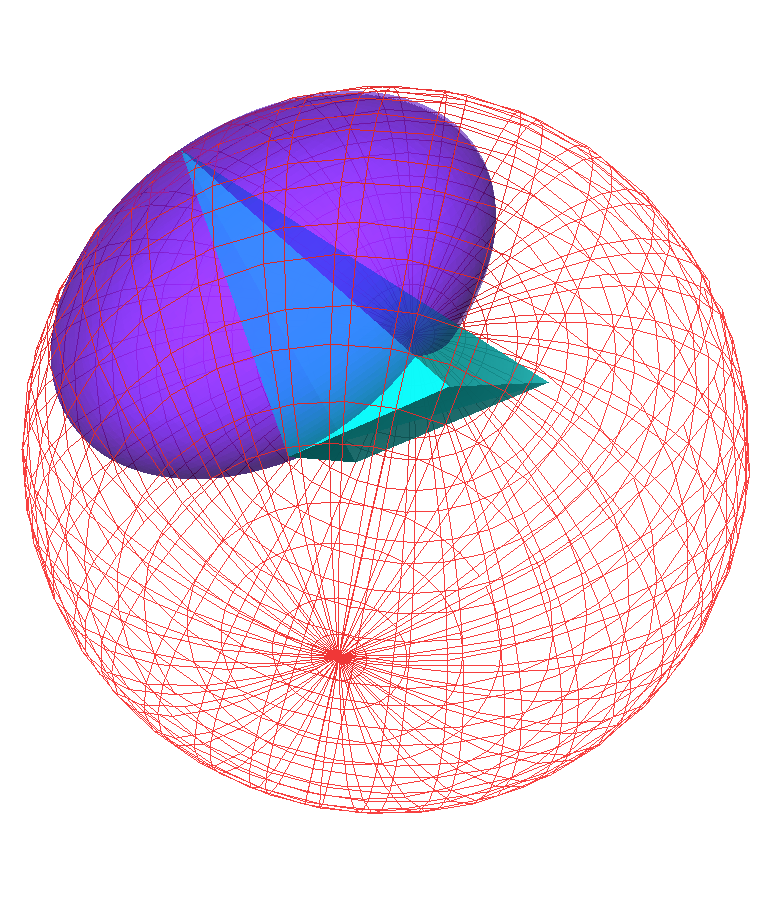
Figure 4: The Horospheres related to the truncated orthoscheme $(\infty,3,3,\infty)$

4.1.1 Horoball packings with two horoball types

We are now focusing on the orthoschemes with the Schläfli symbols $\{\infty,3,6,\infty\}$, $\{\infty,4,4,\infty\}$, $\{\infty,6,3,\infty\}$.

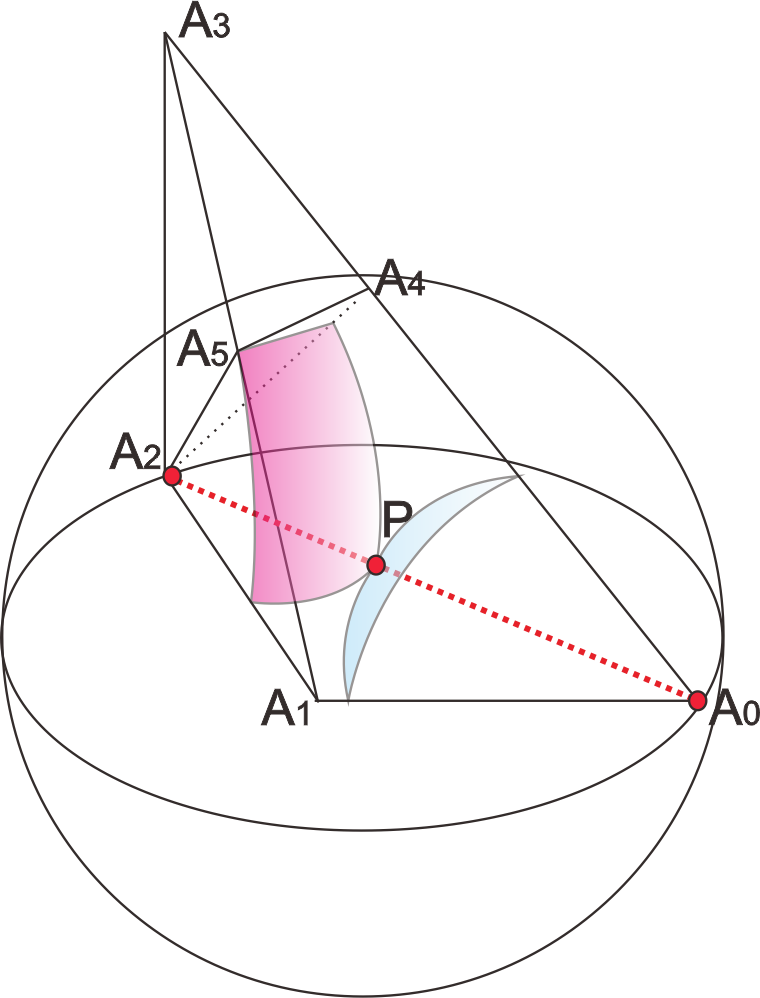
Figure 6: Sketch of two touching horospheres related to the truncated orthoscheme $\{\infty,3,6,\infty\}$

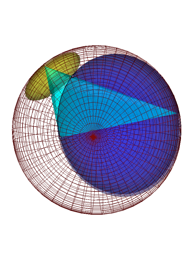
Figure 7: Two touching horospheres related to the truncated orthoscheme $\{\infty,3,6,\infty\}$

In cases when the Coxeter simplex has multiple asymptotic vertices we allow horoballs of different types at different vertices.

Two horoballs of a horoball packing are said to be of the same type or equipack-ed if and only if their local packing densities with respect to a particular cell (in our case a truncated Coxeter orthoscheme) are equal, otherwise the two horoballs are of different types. The set of all horoball types (they are congruent) at a vertex is a one-parameter family. In our investigations we allow horoballs in different types (see [20], [21], [22]).

As in the above subsection, first, we find the bounds for the largest possible horoball type at each vertex lying at the infinity. Such a horoball is tangent to a face that not contains its center. We set one horoball to be of the largest type, and increase the size of the other horoballs until they become tangent. We then vary the types of horoballs within the allowable bounds to find the optimal packing density. The following lemma proved e.g. in [21] gives a relationship between the volumes of two tangent horoball pieces centered at certain vertices of a tiling as we continuously vary their types.

Let $\tau_{1}$ and $\tau_{2}$ be two $n$-dimensional convex pyramid-like regions with vertices at $C_{1}$ and $C_{2}$ sharing a common edge $\overline{C_{1}C_{2}}$. Let $B_{1}(x)$ and $B_{2}(x)$ denote two horoballs centered at $C_{1}$ and $C_{2}$ tangent at the point $I(x)\in{\overline{C_{1}C_{2}}}$. Define the point of tangency $I(0)$ (the “midpoint”) such that the equality $V(0)=2Vol(B_{1}(0)\cap\tau_{1})=2Vol(B_{2}(0)\cap\tau_{2})$ holds for the volumes of the horoball sectors (see Fig. 6).

Lemma 4.3 ([20])

Let $x$ be the hyperbolic distance between $I(0)$ and $I(x)$, then

$$V(x)=Vol(B_{1}(x)\cap\tau_{1})+Vol(B_{2}(x)\cap\tau_{2})=\frac{V(0)}{2}\left(e^{(n-1)x}+e^{-(n-1)x}\right)$$

strictly increases as $x\rightarrow\pm\infty$.

In the considered cases, the truncated orthoschemes have $2$ ideal vertices i.e $A_{2}$ and $A_{0}$ and we construct two horospheres in these vertices. The two horospheres touch each other at the point $P$ lying on the edge $A_{0}A_{2}$ (see Fig. 6). If we move the touching point along edge $A_{0}A_{2}$ the packing density is changing. We can parameterize the possible movement of the touching point $P[\mathbf{p}]$ where $\mathbf{p}(t)=(1-t)\mathbf{a}_{2}+t\mathbf{a}_{0}$. Moreover, these two horospheres could not intersect over their each opposite face, therefore there will be a restriction for parameter $t\in[t_{1},t_{2}]$ (see Fig. 6). Then, for every possible $t$, we have to determine the parameters $s_{i}$ related to both horospheres $\mathcal{B}_{i}$ $(i=0,2)$.

1. Constructing horosphere centered at $A_{2}$. In our setting, the ideal point $A_{2}$ has the coordinate $(1,0,0,1)$, the horosphere could be immediately constructed by applying formula (4.3). To obtain its parameter $s_{1}$, we substitute the coordinates of point $P(t)$ to the equation (4.3) and then solve the expressed quadratic equation for $s_{1}$.

2. Constructing a horosphere centred at $A_{0}$ is not straightforward because the horosphere equations in formula (4.3) holds only for horospheres centred at $A_{2}$. However, we can use a transformation $T$ which is a hyperbolic isometry to transform the center $A_{0}$ and the to $A_{2}=(1,0,0,1)$ and we can apply similar method as formerly substituting the coordinates of $T(P(t))$ to the formula(4.3).

The complete construction is presented in Fig. 6, 7.

Using the formula (4.1) we obtain the following formula for the density of a horoball packing $\mathcal{B}(q,r)$ related to Coxeter orthoscheme tiling $\mathcal{T}(q,r)$:

$$\delta(\mathcal{B}({q,r,t}))=\frac{\sum_{i=1}^{2}Vol(\mathcal{B}_{i}(t)\cap\hat{\mathcal{S}}(q,r))}{Vol(\hat{\mathcal{S}}(q,r))}$$ (4.10)

where $\hat{\mathcal{S}}(q,r)$ denotes the fundamental domain of tiling $\mathcal{T}(q,r)$, and $\mathcal{B}_{i}$ are the horoballs centered at the ideal vertices $A_{0}$ and $A_{2}$ $(q,r)=(3,6),(4,4),(6,3)$. Moreover, $t\in[t_{1}(q,r),t_{2}(q,r)]$ and this intervallum depends on parameters $q,r$ therefore the value of $\delta(\mathcal{B}({q,r,t}))$ is really depends on the parameters $t,q,r$.

4.1.2 Horosphere packing density related to truncated orthoscheme
$\{\infty;3;6;\infty\}$ and $\{\infty;6;3;\infty\}$

In this situations, there is in each case only one possible value of parameters $t$

$$t_{(3,6)}\approx 0.2119416,\leavevmode\nobreak\ t_{(6,3)}\approx 0.5745582.$$

If $(q,r)=(3,6)$ then the horosphere $\mathcal{B}_{2}$ touches the plane $u_{2}$ and $\mathcal{B}_{0}$ touches the face $u_{0}$ and if $(q,r)=(6,3)$ $\mathcal{B}_{2}$ touches the plane $u_{2}$ and $\mathcal{B}_{0}$ touches the face $u_{4}$.

Finally, we obtain the volumes of horoball sectors and the optimal packing densities:

$$\delta_{opt}(\mathcal{B}({3,6,t_{(3,6)}}))=\delta_{opt}(\mathcal{B}({6,3,t_{(6,3)}}))\approx 0.8413392.$$

4.1.3 Horosphere packing density related to truncated orthoscheme
$\{\infty,4;4;\infty\}$

In this case, we obtain that the possible values of $t$ are $t\in[\approx 0.2150<t<\approx 0.3497]$. We obtain the volumes of horoball sectors as the functions of $t$. It is just similar to the previous case, the volume function of horoball sectors centered at $A_{2}$ is increasing function of $t$ if the touching point moving with direction $A_{2}$ to $A_{0}$. While the volume function of horoball sectors centered at $A_{0}$ is decreasing in this situation.

In this case, we realize that the density is increasing as a function of $t$, see Fig.8. Furthermore, the maximum density is attained when $t$ is largest, i.e when the horosphere centered $A_{2}$ touches the opposite face.

$$\delta_{opt}(\mathcal{B}({4,4,t})=\sup\delta(\mathcal{B}({4,4,t}))\approx 0.8188081.$$

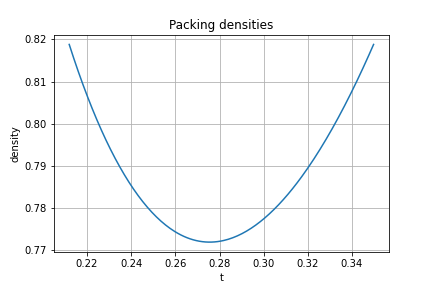
Figure 8: The plot of density function for all possible $t$

The data of packings with two horoball types are summarized in the following table:

Table 4.

Schläfli symbol	$Vol(\mathcal{B}_{i}\cap\hat{\mathcal{S}}(q,r))$	$Vol(\hat{\mathcal{S}}(q,r))$	$\delta_{opt}(\mathcal{B}({q,r}))$.
$(\infty,3,6,\infty)$	0.3608439	0.4228923	0.8413392
$(\infty,4,4,\infty)$	0.3750000	0.4579828	0.8188081
$(\infty,6,3,\infty)$	0.3608439	0.4288923	0.8413392

Finally, we summarize our results of the sphere (inball) packings and the horosphere (horoball) packings in the following

Theorem 4.4

In hyperbolic space $\mathbb{H}^{3}$, between the congruent ball and horoball packings of at most two horoball types, generated by simply truncated Coxeter orthoschemes with parallel faces, the $\mathcal{B}{(3,6)}$ and $\mathcal{B}{(6,3)}$ ball configuration provides the densest packing with density $\approx 0.8413392$.

References

- [1] Bezdek, K.: Sphere Packings Revisited, European Journal of Combinatorics, 27/6 (2006), 864–883.
- [2] Bowen, L. - Radin, C.: Optimally Dense Packings of Hyperbolic Space, Geometriae Dedicata, (2004) 104 , 37–59.
- [3] Bolyai, J.: Appendix, Scientiam Spatii absolute verum exhibens;…, (1831), Marosvásárhely.
- [4] Böhm, J. – Hertel, E: Polyedergeometrie in -dimensionalen Räumen konstanter Krümmung, Birkhäuser, Basel (1981).
- [5] Böröczky, K.: Gömbelhelyezések állandó görbületü terekben I., Math. Lapok, 25, (1974), 265–306.
- [6] Böröczky, K.: Gömbelhelyezések állandó görbületü terekben II., Math. Lapok, 26, (1975), 67–90.
- [7] Böröczky, K.: Packings of spheres in spaces of constant curvature, Acta Math. Acad. Sci. Hungar., 32, (1978), 243–261.
- [8] Böröczky, K. – Florian, A.: Über die dichteste Kugelpackung im hyperbolischen Raum, Acta Math. Acad. Sci. Hungar., 15, (1964), 237–245.
- [9] Eper, M. – Szirmai, J.: Coverings with horo- and hyperballs generated by simply truncated orthoschemes, Submitted manuscript, (2020).
- [10] Fejes Tóth, G. - Kuperberg, W.: Packing and Covering with Convex Sets, Handbook of Convex Geometry Volume B, eds. Gruber, P.M., Willis J.M., pp. 799-860, North-Holland, (1983).
- [11] Fejes Tóth, L.: Regular Figures, Pergamon Press, (1964)
- [12] Hales, T. C. – Ferguson, S. P.: The Kepler conjecture, Discrete and Computional Geometry, 36(1), (2006), 1–269.
- [13] Im Hof, H.-C.: A class of hyperbolic Coxeter groups, Expo. Math., 3, (1985), 179–186.
- [14] Im Hof, H.-C.: Napier cycles and hyperbolic Coxeter groups, Bull. Soc. Math. Belgique, 42, (1990), 523–545.
- [15] M. Jacquemet: The inradius of a hyperbolic truncated n-simplex, Discrete Comput. Geom., 51, (2014), 997–1016.
- [16] Johnson, N.W., Kellerhals, R., Ratcliffe, J.G., Tschants, S.T.: The Size of a Hyperbolic Coxeter Simplex, Transformation Groups, 4/4 (1999), 329–353.
- [17] Kepler, J.: Strena seu de nive sexangula, Frankfurt, Germany: Tampach (1611) Reprinted in Gesammelte Werke (Ed. M. Caspar and F. Hammer, 4 Oxford, England: Clarendon Press (1966)
- [18] Kellerhals, R.: The dilagorithm and volumes of hyperbolic polytopes, AMS Mathematical Surveys and Monographs, 37, (1991), 301–336.
- [19] Kellerhals, R.: On the volume of hyperbolic polyhedra, Math. Ann., 245, (1989), 541–569.
- [20] Kozma, R. T. – Szirmai, J.: Optimally dense packings for fully assymptotic Coxeter tilings by horoballs of different types, Monatsh. Math., 168/1, (2012), 27–47.
- [21] Kozma, R. T. – Szirmai, J.: New lower bound for the optimal ball packing density of hyperbolic 4-space, Discrete Comput. Geom., (2014), DOI: 10.1007/s00454-014-9634-1
- [22] Kozma, R. T. – Szirmai, J.: New horoball packing density lower bound in hyperbolic 5-space, Geometriae Dedicata, (2019), DOI: 10.1007/s10711-019-00473-x, arXiv:1809.05411
- [23] Kozma, R. T. – Szirmai, J.: Horoball packing density lower bounds in higher dimensional hyperbolic -space for , Submitted Manuscript, (2019), arXiv:1907.00595
- [24] Kozma, R. T. – Szirmai, J.: The structure and visualization of optimal horoball packings in 3-dimensional hyperbolic space, Submitted Manuscript, (2016), arXiv:1601.03620, (Appendix: http://homepages.math.uic.edu/rkozma/SVOHP.html))
- [25] Marshall, T. H.: Asymptotic Volume Formulae and Hyperbolic Ball Packing, Annales Academic Scientiarum Fennica: Mathematica, 24 (1999), 31–43.
- [26] Molnár, E.: The projective interpretation of the eight 3-dimensional homogeneous geometries, Beitr. Algebra Geom., (1997), 38), 261–288.
- [27] Molnár, E. – Stojanovic, M. – Szirmai, J.: Non-fundamental trunc-simplex tilings and their optimal hyperball packings and coverings in hyperbolic space, Submitted Manuscript (2020)
- [28] Molnár, E. – Szirmai, J.: Top dense hyperbolic ball packings and coverings for complete Coxeter orthoscheme groups, Publications de L’institut Mathématique, 103(117), (2018), 129–146, DOI: 10.2298/PIM1817129M
- [29] Rogers, C.A.: Packing and Covering, Cambridge Tracts in Mathematics and Mathematical Physics 54, Cambridge University Press, (1964).
- [30] Szirmai, J.: Congruent and non-congruent hyperball packings related to doubly truncated Coxeter orthoschemes in hyperbolic 3-space, Acta Univ. Sapientiae, Mathematica, 11, 2 (2019), 437–459.
- [31] Szirmai, J.: Horoball packings to the totally assymptotic regular simplex in the hyperbolic -space, Aequat. Math., 85, (2013), 471–482, DOI: 10.1007/s00010.012-0158-6.
- [32] Szirmai, J.: Horoball packings and their densities by generalized simplicial density function in the hyperbolic space, Acta Math. Hung., 136/1-2, (2012), 39–55, DOI: 10.1007/s10474-012-0205-8.
- [33] Szirmai, J.: Horoball packings related to the 4-dimensional hyperbolic 24 cell honeycomb , Filomat, 32/1, (2018), 87–100, DOI: 10.2298/FIL1801087S, arXiv:1502.02107.
- [34] Szirmai, J.: Hyperball packings in hyperbolic 3-space, Matematicki Vesnik, 70/3, (2018), 211–221, arXiv:1405.0248.
- [35] Szirmai, J.: Density upper bound of congruent and non-congruent hyperball packings generated by truncated regular simplex tilings, Rendiconti del Circolo Matematico di Palermo Series 2, 67, (2018), 307–322, DOI: 10.1007/s12215-017-0316-8, arXiv:1510.03208.
- [36] Szirmai, J.: Hyperball packings related to octahedron and cube tilings in hyperbolic space, Contributions to Discrete Mathematics, 15/2, (2020), 42-59, arXiv:1803.04948.
- [37] Szirmai, J.: The optimal hyperball packings related to the smallest compact arithmetic 5-orbifolds, Kragujevac Journal of Mathematics, 40/2, (2016), 260–270, DOI: 10.5937/KgJMath1602260S, arXiv:1326.4221.
- [38] Szirmai, J.: The -gonal prism tilings and their optimal hypershphere packings in the hyperbolic 3-space, Acta Math. Hung., 111(1-2), (2006), 65–76.
- [39] Szirmai, J.: The least dense hyperball covering to the regular prism tilings in the hyperbolic -space, Ann. Mat. Pur. Appl., 195/1, (2016), 235–248, DOI: 10.1007/s10231-014-0460-0.
- [40] Szirmai, J.: Packings with horo- and hyperballs generated by simple frustum orthoschemes, Acta Math. Hungar., 152(2), (2017), 365–382, DOI: 10.1007/s10474-017-0728-0.
- [41] Szirmai, J.: Decomposition method related to saturated hyperball packings, Ars Mathematica Contemporanea, 16, (2019), 349–358, DOI: 10.26493/1855-3974.14850b1, arXiv:1709.04369.
- [42] Szirmai, J.: Upper bound of density for packing of congruent hyperballs in hyperbolic 3-space, Submitted manuscript, (2020), arXiv:1812.06785.
- [43] Vermes, I.: Ausfüllungen der hyperbolischen Ebene durch kongruente Hyperzykelbereiche, Period. Math. Hungar., 10/4, (1979), 217–229.
- [44] Vermes, I.: Über reguläre Überdeckungen der Bolyai-Lobatschewskischen Ebene durch kongruente Hyperzykelbereiche, Period. Math. Hungar., 25/3, (1981), 249–261.
- [45] Vermes, I.: Bemerkungen zum Problem der dünnesten Überdeckungen der hyperbolischen Ebene durch kongruente Hyperzykelbereiche, Studia Sci. Math. Hungar., 23, (1988), 1–6.