Sr and Ba abundance determinations: comparing machine-learning with star-by-star analyses

Abstract

Context. A new large sample of 895 s-process-rich candidates out of 454 180 giant stars surveyed by LAMOST at low spectral resolution ($R\sim 1800$) has been reported by Norfolk et al. (2019; hereafter N19).

Aims. We aim at confirming the s-process enrichment at the higher resolution ($R\sim 86\;000$) offered by the HERMES-Mercator spectrograph, for the 15 brightest targets of the previous study sample which consists in 13 Sr-only stars and two Ba-only stars (this terminology designates stars with either only Sr or only Ba lines strengthened).

Methods. Abundances were derived for elements Li, C (including ¹²C/¹³C isotopic ratio), N, O, Na, Mg, Fe, Rb, Sr, Y, Zr, Nb, Ba, La, and Ce, using the TURBOSPECTRUM radiative transfer LTE code with MARCS model atmospheres. Binarity has been tested by comparing the Gaia DR2 radial velocity (epoch 2015.5) with the HERMES velocity obtained 1600 - 1800 d (about 4.5 years) later.

Results. Among the 15 programme stars, four show no s-process overabundances ([X/Fe] $<0.2$ dex), eight show mild s-process overabundances (at least three heavy elements with $0.2<\rm{[X/Fe]}<0.8$), and three have strong overabundances (at least three heavy elements with [X/Fe] $\geq$ 0.8). Among the 13 stars classified as Sr-only by the previous investigation, four have no s-process overabundances, eight are mild barium stars, and one is a strong barium star. The two Ba-only stars turn out to be both strong barium stars. Especially noteworthy is the fact that these two are actually dwarf barium stars. Two among the three strong barium stars show clear evidence for being binaries, as expected for objects produced through mass-transfer. The results for the no s-process and mild barium stars are more surprising. Among the no-s stars, there are two binaries out of four, whereas only one out of the eight diagnosed mild barium stars show a clear signature of radial-velocity variations.

Conclusions. Blending effects and saturated lines have to be considered very carefully when using machine-learning techniques, especially on low-resolution spectra. Among the Sr-only stars from the previous study sample, one may expect about 60% (8/13) of them to be true mild barium stars and about 8% to be strong barium stars, and this fraction is likely close to 100% for the previous study Ba-only stars (2/2). It is therefore recommended to restrict to the previous study Ba-only stars when one needs an unpolluted sample of mass-transfer (i.e., extrinsic) objects.

1 Introduction

Barium (Ba) stars or Ba II stars, as they were originally named, are G- and K-type giants with strong absorption lines of slow-neutron-capture (s)-process elements in their spectra, in combination with enhanced carbon-bearing molecular bands. They were first identified as chemically peculiar by Bidelman & Keenan (1951), who discussed their distinctive spectroscopic characteristics and stressed the extraordinary strength of the resonance line of ionised barium at 4554 Å. The resulting overabundance of barium and other s-process elements on the surface of these stars could not be explained from an evolutionary point of view because the s-process of nucleosynthesis takes place in the interiors of Asymptotic Giant Branch (AGB) stars, whereas Ba stars are instead dwarf, subgiant, red-giant-branch (RGB), or red-clump stars (e.g., Jorissen et al., 2019; Escorza et al., 2019). Barium stars are understood to originate from a binary evolution channel (McClure, 1983). According to this formation scenario, the carbon and the s-process elements were transferred to the current primary from a more evolved companion when the latter was in its AGB phase.

Galactic chemical evolution provides an alternative explanation for mild barium stars (with [Ba/Fe] $\sim 0.2-0.3$ dex), which represent the upper [Ba/Fe] tail of the Galactic ([Ba/Fe],[Fe/H]) trend (e.g. Edvardsson et al., 1993; Tautvaišienė et al., 2021).

Since recently, the largest homogeneous sample of barium stars was collected in the course of the Michigan Spectral Sky Survey, with 205 new discovered barium stars (MacConnell et al., 1972). Mainly based on this sample, Lü et al. (1983) then built their catalogue with 221 entries, followed by an updated version with 389 stars (Lü, 1991). However, a substantial fraction of them are probably not barium stars (especially those classified with a Ba index $\leq 1$; e.g., Smiljanic et al., 2007).

More recently, large-field spectroscopic surveys like LAMOST (Wu et al., 2011; Bai et al., 2016), involving low-resolution spectroscopy, have permitted to potentially increase in a tremendous manner the number of known stars with enhanced s-process elements. For instance, Norfolk et al. (2019, hereafter N19), have reported 859 candidates (out of 454 180 giants studied) which were classified as either Sr-only, or Ba-only, or Ba- and Sr-strong. This classification was based on the comparison between the strengths of the most conspicuous Sr ii (4077 and 4215 Å ) and Ba ii lines (4554, 4934, and 6496 Å ) in template and target stars, using the machine-learning technique ”The Cannon” (Ness et al., 2015). There are however several caveats (as we discuss below) with this approach, which call for an a posteriori verification of the s-process enhancement from high-resolution spectra. Only one star was subject to such a check by N19.

The purpose of this paper is to perform such a verification on a larger sample of 15 stars. The motivation thereof is the very low resolution of LAMOST spectra ($R\sim 1800$) combined with the fact that the above-mentioned lines of Sr ii and Ba ii are known to show a positive luminosity effect (i.e., strengthening of the line due to low gravity rather than overabundance; Gray et al., 2009). Moreover, some of those lines are blended (e.g., Sr II 4215.5 Å  by CN lines) and are often saturated, in which case they become poor abundance diagnostics.

Recently, the Sr abundance in Carbon-Enhanced Metal-Poor (CEMP) stars has gained a lot of attention since some studies (Hansen et al., 2016, 2019) found that the Sr/Ba ratio can be used to separate CEMP stars into their sub-groups (CEMP-no, CEMP-s, and CEMP-rs) and to identify their progenitors since this ratio depends on the nucleosynthetic sites.

Large field spectroscopic surveys have provided spectra for millions of stars and machine-learning techniques are widely used to measure abundances of the elements. Our current analysis aims at discussing the difficulties in measuring the abundances of Ba and Sr especially when using machine-learning techniques on low-resolution spectra.

In this paper, we present a detailed high-resolution spectroscopic analysis of the brightest s-process-rich candidates of N19 in order (i) to check for possible misclassification as (mild) barium stars, (ii) to understand the origin of the variations in their individual elemental abundance pattern and thereby understand the origin of these peculiar abundances, and (iii) to evaluate the power of machine-learning techniques for abundance determination from low-resolution spectra.

This paper is organized as follows. Section 2 describes the selection of the sample. Section 3 discusses the method used for deriving the atmospheric parameters. Section 4 presents the abundance analysis. Section 5 compares N19 classification with ours, whereas Sect. 6 presents comments about individual stars. Section 7 discusses the possible origin of the peculiarities of the different identified classes, and finally Sect. 8 discusses the efficiency with which the machine-learning method The Cannon has been able to correctly flag s-process-enriched stars from low-resolution spectra. Conclusions are presented in Sect. 9.

2 Sample selection

Our analysis focuses on the brightest among the stars from N19 tagged as ’Sr only’ or ’Ba only’ candidates (this terminology designates stars with either only Sr or only Ba lines strengthened, respectively; see Sects. 4.3 and 4.4), visible from the Roque de los Muchachos Observatory in La Palma, Canary Islands (Spain). They are listed in Table 1 along with N19 classification. They were observed with the high-resolution HERMES spectrograph (Raskin et al., 2011) mounted on the 1.2m Mercator telescope. The spectra covers the spectral range 3900 – 9000 Å  with a resolution of 86,000. The S/N ratio of the HERMES spectra around 5000 Å  is listed in Table 1.

3 Derivation of atmospheric parameters

The atmospheric parameters of the programme stars were derived following the same method as outlined by Karinkuzhi et al. (2018). We used the BACCHUS (Brussels Automatic Code for Characterizing High accUracy Spectra) tool in a semi-automated mode (Masseron et al., 2016). BACCHUS combines interpolated MARCS model atmospheres (Gustafsson et al., 2008) with the 1D local-thermodynamical-equilibrium (LTE) spectrum-synthesis code TURBOSPECTRUM (Alvarez & Plez, 1998; Plez, 2012). We manually selected Fe I and Fe II lines so as to choose blending-free lines for BACCHUS to derive the stellar parameters ($T_{\rm eff}$, [Fe/H], $\log g$, microturbulence velocity $\xi$ as well as rotational velocity). The code includes on the fly spectrum synthesis, local continuum normalization, estimation of local S/N ratio and automatic line masking. It computes abundances using equivalent widths or spectral synthesis, allowing to check for excitation and ionization equilibria, thereby constraining $T_{\rm eff}$ and $\log g$. The microturbulent velocity $\xi$ is calculated by ensuring consistency between Fe abundances derived from lines of various reduced equivalent widths.

Table 1: Programme stars and adopted atmospheric parameters.

Name	$T_{\rm eff}$	$\log g$	[Fe/H]	$\xi$	S/N	Class
	(K)	(cm s-2)	(dex)	(km s-1)
no s-process enrichment
HD 7863	4637 $\pm$ 64	2.29 $\pm$ 0.40	$-$0.07 $\pm$ 0.05	1.26 $\pm$ 0.10	68	no
	4561 $\pm$ 6	2.37 $\pm$ 0.01	0.13 $\pm$ 0.01	2	–	Sr only
HIP 69788	5127 $\pm$ 11	3.90 $\pm$ 0.14	$-$0.04 $\pm$ 0.04	0.61 $\pm$ 0.10	75	no
	4913 $\pm$ 10	3.04 $\pm$ 0.02	$-0.34\pm 0.01$	2	–	Sr-only
TYC 3144$-$1906$-$1	4136 $\pm$ 64	1.89 $\pm$ 0.50	$-$0.13 $\pm$ 0.10	1.37 $\pm$ 0.04	48	no (Li)
	4232 $\pm$ 8	1.87 $\pm$ 0.02	0.15 $\pm$ 0.01	2	–	Sr only
TYC 4684$-$2242$-$1	4651 $\pm$ 20	2.70 $\pm$ 0.14	$-$0.05 $\pm$ 0.07	1.15 $\pm$ 0.05	54	no
	4652 $\pm$ 12	2.71 $\pm$ 0.03	0.05 $\pm$0.02	2	–	Sr only
mild s-process enrichment
BD $-07^{\circ}$ 402	4654 $\pm$ 6	2.62 $\pm$ 0.19	$-$0.11 $\pm$ 0.05	1.22 $\pm$ 0.10	61	mild (Li-rich)
	4688 $\pm$ 9	2.58 $\pm$ 0.02	0.11 $\pm$ 0.01	2	–	Sr only
BD $+44^{\circ}$ 575	4175 $\pm$ 6	1.50 $\pm$ 0.19	$-$0.45 $\pm$ 0.05	1.60 $\pm$ 0.10	76	mild
	4202 $\pm$ 12	1.59 $\pm$ 0.03	$-0.11\pm 0.02$	2	–	Sr only
TYC 22$-$155$-$1	4704 $\pm$ 9	3.10 $\pm$ 0.32	$-$0.20 $\pm$ 0.10	1.04 $\pm$ 0.05	47	mild
	4629 $\pm$ 11	2.72 $\pm$ 0.03	$-0.22\pm 0.01$	2	–	Sr only
TYC 2913$-$1375$-$1	4757 $\pm$ 69	2.00 $\pm$ 0.30	$-$0.61 $\pm$ 0.11	1.45 $\pm$ 0.05	32	mild
	4791$\pm$ 15	2.41$\pm$ 0.04	$-0.37\pm 0.02$	2	–	Sr only
TYC 3305$-$571$-$1	4816 $\pm$ 3	2.76 $\pm$ 0.16	$-$0.05 $\pm$ 0.08	1.31 $\pm$ 0.04	49	mild
	4798 $\pm$ 8	2.62 $\pm$ 0.02	0.18 $\pm$ 0.01	2	–	Sr only
TYC 752$-$1944$-$1	5069 $\pm$ 25	2.94 $\pm$ 0.05	$-$0.08 $\pm$ 0.08	1.33 $\pm$ 0.04	61	mild
	4967 $\pm$ 11	2.79 $\pm$ 0.03	0.02 $\pm$ 0.01	2	–	Sr only
TYC 4837$-$925$-$1	4679 $\pm$ 34	2.16 $\pm$ 0.29	$-$0.27 $\pm$ 0.07	1.30 $\pm$ 0.04	44	mild
	4739 $\pm$ 14	2.46 $\pm$ 0.04	0.02 $\pm$ 0.02	2	–	Sr only
TYC 3423$-$696$-$1	5042 $\pm$ 64	3.66 $\pm$ 0.30	0.02 $\pm$ 0.08	0.96 $\pm$ 0.04	55	mild
	5014 $\pm$ 17	3.59 $\pm$ 0.03	0.22 $\pm$ 0.02	2	–	Sr only
strong s-process enrichment
TYC 2250$-$1047$-$1	5335 $\pm$ 25	3.71 $\pm$ 0.18	$-$0.55 $\pm$ 0.12	1.45 $\pm$ 0.05	32	strong
	5097 $\pm$ 23	3.25 $\pm$ 0.03	$-0.68\pm 0.03$	2	–	Ba only
TYC 2955$-$408$-$1	4716 $\pm$ 64	2.49 $\pm$ 0.3	$-$0.39 $\pm$ 0.08	1.25 $\pm$ 0.04	61	strong
	4724 $\pm$ 10	2.39 $\pm$ 0.03	$-0.21\pm 0.01$	2	–	Sr only
TYC 591$-$1090$-$1	5267 $\pm$ 36	3.68 $\pm$ 0.50	$-$0.30 $\pm$ 0.12	1.18 $\pm$ 0.06	28	strong
	5106 $\pm$ 13	3.33 $\pm$ 0.02	$-0.29\pm 0.01$	2	–	Ba only

4 Abundance analysis

Abundances are derived by comparing observed and synthetic spectra generated with the TURBOSPECTRUM code. The solar abundances are taken from Asplund et al. (2009). We used the line lists assembled in the framework of the Gaia-ESO survey (Heiter et al., 2015; Heiter, 2020). These lines are presented in Karinkuzhi et al. (2018, 2021), hence we do not list them again here. The abundances are derived under the LTE assumption, but a posteriori NLTE corrections have been added whenever available, as we discuss below. In Table 5 and 2, we present all the abundances derived from our target stars. In the following, we comment on individual elemental abundances.

4.1 Li

The Li abundance has been derived from the Li I 6707 Å  line. We could measure the Li abundance in only two stars, TYC 3144$-$1906$-$1 and BD $-07^{\circ}$402 with $\log\epsilon({\rm Li})\approx 0.6$ and 1.3 dex respectively (Table 2). These values are in accordance with the Li abundance of 1.0 dex predicted in RGB after the first dredge up (e.g., Jorissen et al., 2020, and references therein)

4.2 C, N, and O

We derive oxygen abundances from the [O I] line at 6300.303 Å  except for TYC 591$-$1090$-$1 where the O I resonance triplet at 7774 Å  is used instead. A non-LTE correction of 0.2 dex has been applied to obtain the final adopted O abundance for this object (Asplund et al., 2005; Amarsi et al., 2016). In TYC 2913$-$1375$-$1 and TYC 3144$-$1906$-$1, we could detect neither the 6300.303 Å  line nor the 7774 Å  line. Hence we used another $\alpha$-element, namely Ca, and adopted [Ca/Fe] as a proxy for [O/Fe] (Table  5).

The carbon abundance is obtained mainly from the CH band at 4310 Å  and from the C₂ bands at 5165 and 5635 Å. Since our programme stars do not show strong enrichment of carbon, the C₂ bands are not saturated. We could derive consistent abundances from these three bands.

The nitrogen abundance for the programme stars are derived from the CN bands above 7500 Å. The ¹²C/¹³C ratio is derived using ¹²CN features at 8003.553 and 8003.910 Å , and ¹³CN features at 8004.554, 8004.728, 8004.781, 8010.458, and 8016.429 Å. For several stars, the signal-to-noise ratio was not high enough to enable us to estimate the ¹²C/¹³C ratio.

4.3 Light s-process elements: Sr, Y and Zr

The Y abundances for the programme stars are determined from the Y II lines. The Zr abundance is derived using Zr I and Zr II lines, which yield consistent abundances.

We now present a detailed discussion of all the lines involved in the Sr abundance determination, either by us or by N19, as Sr is a key element in N19 barium-star diagnostic. In the present work, the Sr abundance is estimated using the Sr I lines at 4607.327 Å  (resonance line), 4811.877 Å  (non-resonant) and 7070.070 Å  (non resonant).

For the Sr I line at 4811.877 Å  (not used by Karinkuzhi et al., 2018, 2021), a $\log gf$ of 0.190 has been used (García & Campos, 1988). For the 4607.327 Sr I line, Hansen et al. (2013) advocate the value of 0.283 for its $\log gf$ (from Parkinson et al., 1976), because it allows to match the solar Sr abundance. An analysis of the HERMES Arcturus spectrum shows a similar agreement as for the Sun, as revealed by the first line of Table 3. Adopting a metallicity of $-0.62$ for Arcturus (Maeckle et al., 1975), the 4607 and 4812 lines yield [Sr/Fe] = $-0.43$ and $-0.20$, respectively, in agreement with Maeckle et al. (1975) who found [Sr/Fe] $=-0.4\pm 0.3$ dex.

The Sr I line at 4607.327 Å is known to form under NLTE conditions (Bergemann et al., 2012; Hansen et al., 2013), and the former authors list in their Table 3 the NLTE corrections for this line at metallicities 0.0 and $-$0.60 for various temperatures and surface gravities. The atmospheric parameters of all our programme stars are within this range, and the corresponding NLTE corrections vary between 0.1 and 0.27 dex. In Table 3, we list separately the abundances derived from the three clean (i.e., unblended and not saturated) Sr lines, namely Sr I 4607.327, 4811.877 Å  and 7070.070 Å, along with the NLTE correction (between parentheses) applied to the LTE abundance from the 4607 line (for the latter line, Table 3 lists the NLTE abundance). Table 2 provides the average [Sr/Fe] abundance as derived from these three lines.

To derive the Sr abundances, N19 used instead the Sr II lines at 4077.077 and 4215.519 Å. In stars of solar and mildly subsolar metallicities, as it is the case for all the programme stars, these lines are however saturated (Fig. 1; see also Hansen et al., 2013), and could not be used to derive abundances.

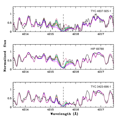
Figure 1: The Sr II 4077.7 Å  (top panel) and Sr II 4215.5 Å  (bottom panel) lines are shown in three N19 ”Sr-only” stars. The magenta, blue, red, green and turquoise lines correspond to $\log\epsilon$(Sr) = 3.6, 3.3, 3.0, 2.7 and 2.4 dex, respectively. The brown line is for no Sr. These lines are clearly saturated.

Nevertheless, for the sake of comparison, Table 3 lists the Sr abundances provided by N19 for these lines, along with our very uncertain abundance estimate from the 4077.077 Å  line. The 4215.519 Å  line could not be used to derive even a rough abundance estimate as the spectrum syntheses for the different abundances lie on top of each other (Fig. 1). This situation is due to the presence of the strong CN bandhead at $\lambda$ 4216 Å  (Sect. 27 of Gray et al., 2009), which strongly depresses the continuum, especially in stars with enhanced C or N. Figure 2 shows the strong impact of the CN band in the 4215 Å   region, even in the absence of the Sr line. Note especially how the ”no Sr + CN” (top panel) and ”Sr + CN” (bottom panel) are barely distinguishable, even at the high resolution of HERMES, which is nearly 50 times the one of LAMOST.

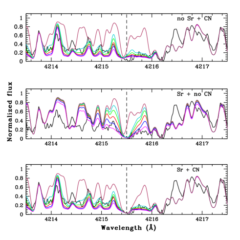
Figure 2: Spectral syntheses of the 4214 – 4217 Å   wavelength range surrounding the Sr II 4215.5 Å  line in HD 7863. In the top panel, the spectral syntheses do not include the Sr II 4215.5 Å  line, to reveal the impact of the 4216 Å CN band head. The magenta, blue, red, green and turquoise lines correspond to $\log\epsilon$ (N)  = 9.15, 8.85, 8.55, 8.25 and 7.95 dex, respectively. In the middle panel, the contribution from the CN band is removed and spectral syntheses are done by varying only the Sr abundance. In this case, the magenta, blue, red, green and turquoise lines correspond to $\log\epsilon$ (Sr)  = 3.6, 3.3, 3.0, 2.7 and 2.4 dex, respectively. In the bottom panel, the synthesis includes both Sr and CN, with the adopted N abundance of $\log\epsilon$(N) = 8.55. The color-coding of the Sr abundance is the same as in the middle panel. The adopted ¹²C/¹³C ratio is 19.

In this respect, it is certainly relevant to note that the three no-s stars, considered as Sr-only by N19 (TYC 3144$-$1906$-$1, TYC 4684$-$2242$-$1, and HD 7863; see Table 1 and Sect. 5), are precisely those being N-rich (Fig. 3).

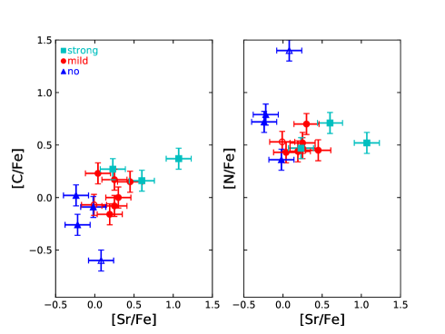
Figure 3: The correlation between the [Sr/Fe] index and the C and N abundances, showing a clear N overabundance for three among the four Sr-no stars (see Sect. 5.

Table 2: Line by line abundances of Sr and Ba in the programme stars.

	[Sr I/H]				[Sr II/H]			[Ba II/H]
$\lambda$(Å )	4607.33	4811.88	7070.07		4077.08	4215.52		4524.92	4554.03	4934.08	5853.67	6141.67
Arcturus	$-$1.05 (0.27)	$-$0.82
	no s-process enrichment
HD 7863	$-$0.27 (0.2)	$-$0.27	$-$0.27		$-$0.17:	–		0.12	$-$0.18:	–	$-$0.18	$-$0.18
	–	–	–		0.9	0.9		–	0.0	0.1	–	–
HIP 69788	$-$0.22 (0.1)	0.13	–		$-$0.17:	–		–	0.12:	0.12:	0.12	–
	–	–	–		0.7	0.5		–	0.7	0.4	–	–
TYC 3144$-$1906$-$1	–	$-$0.12	$-$0.02		$-$0.17:	–		–	0.12:	0.12:	$-$0.18	$-$0.18
	–		–		1.0	1.0		–	0.2	0.0	–	–
TYC 4684$-$2242$-$1	$-$0.57 (0.2)	–	$-$0.02		0.13:	–		–	0.12:	0.12:	0.02	0.02
	–	–	–		0.9	0.9		–	-0.1	0.0	–	–
	mild s-process enrichment
BD $-07^{\circ}$402	$-$0.27 (0.2)	0.12	$-$0.17		0.13:	–		–	0.12:	0.22:	0.1	0.1
	–	–	–		0.9	1.0		–	0.0	-0.1	–	–
BD +44∘575	–	$-$0.2	$-$0.17		$-$0.17:	–		–	0.12:	0.12:	$-$0.2	–
	–	–	–		0.9	0.8		–	$-$0.2	$-$0.1	–	–
TYC 22$-$155$-$1	$-$0.37 (0.2)	$-$0.2	0.13		$-$0.17:	–		0.3:	0.12:	0.12:	0.1	0.1
	–	–	–		0.5	0.5		–	-0.2	-0.3	–	–
	–	–	–		0.2	0.4		–	$-$0.3	$-$0.5	–	–
TYC 2913$-$1375$-$1	–	–	–		–	–		–	$-$0.18	$-$0.03:	$-$0.68	$-$0.68
	–	–	–		0.2	0.4		–	$-$0.3	$-$0.5	–	–
TYC 3305$-$571$-$1	0.30 (0.2)	–	0.13:		–	–		–	0.42:	–	0.32	0.32
	–	–	–		0.9	0.9		–	0.2	0.1	–	–
TYC 752$-$1944$-$1	0.03 (0.1)	–	0.43		–	–		–	0.62:	0.62:	0.52	0.52
	–	–	–		0.8	0.8		–	0.3	0.0	–	–
TYC 4837$-$925$-$1	$-$0.27(0.2)	–	0.13		$-$0.17:	–		–	0.12:	0.12:	$-$0.18	$-$0.18
	–	–	–		0.8	0.8		–	0.0	-0.1	–	–
TYC 3423$-$696$-$1	0.53: (0.1)	0.43	–		$-$0.17:	–		–	0.12:	0.12:	0.0	0.1
	–	–	–		0.8	0.9		–	0.1	0.2	–	–
	strong s-process enrichment
TYC 2250$-$1047$-$1	0.33 (0.2)	0.73	–		–	–		0.62	0.82:	0.82:	0.62	0.62
	–	–	–		-0.8	-0.7		–	0.3	0.3	–	–
TYC 2955$-$408$-$1	0.03 (0.2)	–	0.43		0.13:	–		0.6	0.52:	0.52:	0.52	0.52
	–	–	–		0.7	0.6		–	0.2	-0.2	–	–
TYC 591$-$1090$-$1	$-$0.07 (0.1)	–	–		–	–		0.9	0.82:	0.82:	0.6	–
	–	–	–		0.5	-0.4		–	0.7	0.7	–	–

4.4 Heavy s-process elements: Ba, La, Ce

We derived Ba abundances in most of the programme stars using the Ba II lines at 5853.673 and 6141.673 Å. For a few objects, as these lines are strong and saturated, the Ba abundance is estimated from the spectral synthesis of the weak Ba II line at 4524.924 Å. Ba lines are strongly affected by hyperfine (HF) splitting. HF splitting data is not available for the 4524.924 Å  line, but it was taken into account for the Ba II 5853.673 Å  line.

The Ba II lines at 4554.03 and 4934.08 Å  are saturated (Fig. 4) and were therefore not considered to derive Ba abundances. Nevertheless, they were used by N19, and are listed in Table 3. When comparing the derived Ba abundances, we conclude that the agreement between the N19 study and ours is much better for Ba than for Sr.

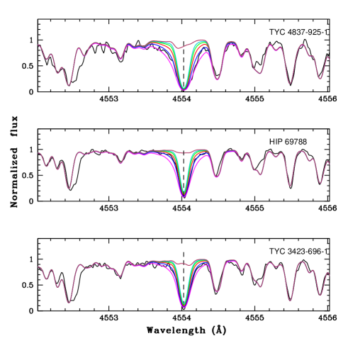
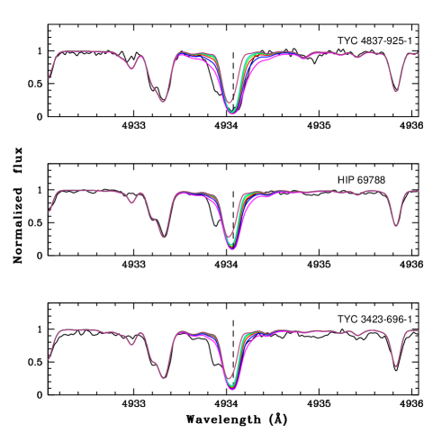
Figure 4: The Ba II 4554.026 Å  (top panel) and Ba II 4934.076 Å  lines (bottom panel) are shown in three N19 Sr-only stars. The magenta, blue, red, green and cyan curves correspond to $\log\epsilon$(Ba) = 2.6, 2.3, 2.0, 1.7 and 1.4 dex respectively. The brown curve is for no Ba.

The La abundance is determined mainly using the lines for which HF splitting is available.

As we mentioned earlier, all the lines used are listed in Karinkuzhi et al. (2018, 2021) along with the hfs splitting and isotopic shifts as listed in these references.

4.5 Abundance uncertainties

Abundance uncertainties are calculated for all elements using the methodology described in Karinkuzhi et al. (2018, 2021). Following Eq. 2 from Johnson (2002), the uncertainties on the elemental abundances $\log\epsilon$ write:

$$\begin{split}\sigma^{2}_{\rm tot}=\sigma^{2}_{\rm ran}\;+\;\left(\frac{\partial\log\epsilon}{\partial T}\right)^{2}\sigma^{2}_{T}\;+\;\left(\frac{\partial\log\epsilon}{\partial\log g}\right)^{2}\;\sigma^{2}_{\log g}\\ \;+\;\left(\frac{\partial\log\epsilon}{\partial\xi}\right)^{2}\;\sigma^{2}_{\xi}\;+\;\left(\frac{\partial\log\epsilon}{\partial\mathrm{[Fe/H]}}\right)^{2}\sigma^{2}_{\mathrm{[Fe/H]}}\;+\;\\ 2\bigg{[}\left(\frac{\partial\log\epsilon}{\partial T}\right)\left(\frac{\partial\log\epsilon}{\partial\log g}\right)\sigma_{T,\log g}\;+\;\left(\frac{\partial\log\epsilon}{\partial\xi}\right)\left(\frac{\partial\log\epsilon}{\partial\log g}\right)\sigma_{\log g,\xi}\\ \;+\;\left(\frac{\partial\log\epsilon}{\partial\xi}\right)\left(\frac{\partial\log\epsilon}{\partial T}\right)\sigma_{\xi,T}\Bigg{]},\end{split}$$ (1)

where $\sigma_{T}$, $\sigma_{\log g}$, and $\sigma_{\xi}$ are the typical uncertainties on the atmospheric parameters and are derived by taking the average of the errors listed in Table 1 corresponding to each atmospheric parameter. These values are estimated as $\sigma_{T}$ = 33 K, $\sigma_{\log g}$ = 0.26 dex, $\sigma_{\xi}$ = 0.06 km/s. The uncertainty on metallicity was estimated as $\sigma_{\mathrm{[Fe/H]}}$ = 0.08 dex. The partial derivatives appearing in Eq. 1 were evaluated in the specific cases of BD $-07^{\circ}$ 402, varying the atmospheric parameters $T_{\rm eff}$, $\log g$, microturbulence $\xi$, and [Fe/H] by 100 K, 0.5, 0.5 km/s and 0.5 dex, respectively. The resulting changes in the abundances are presented in Table 3. The covariances $\sigma_{T,\log g}$, $\sigma_{\log g,\xi}$, and $\sigma_{\xi,T}$ are derived by the same method as given by Johnson (2002). In order to calculate $\sigma_{T,\log g}$, we varied the temperature while fixing metallicity and microturbulence, and determined the $\log g$ value required for ensuring the ionization balance. Then using Eq. 3 of Johnson (2002), we derived the covariance $\sigma_{T,\log g}$ and found a value of 1.62. In a similar way, we found $\sigma_{\log g,\xi}$ = $-$0.02 and $\sigma_{\xi,T}$ = 0.75.

The random error $\sigma_{\rm ran}$ is the line-to-line scatter. For most of the elements, we could use more than four lines to derive the abundances. In that case, we have adopted $\sigma_{\mathrm{ran}}=\sigma_{l}/N^{1/2}$, where $\sigma_{l}$ is the standard deviation of the abundances derived from all the $N$ lines of the considered element. For the elements for which fewer number of lines are used to derive the abundances, we selected a $\sigma_{\rm ran}$ value as described in Karinkuzhi et al. (2021). The final error on [X/Fe] is derived from

$$\sigma^{2}_{\rm[X/Fe]}=\sigma^{2}_{\rm X}+\sigma^{2}_{\rm Fe}-2\;\sigma_{\rm X,Fe},$$ (2)

where $\sigma_{\rm X,Fe}$ is calculated using Eq. 6 from Johnson (2002) with an additional term including $\left(\frac{\partial\log\epsilon}{\partial\mathrm{[Fe/H]}}\right)$.

Table 3: Sensitivity of the abundances ($\Delta\log\epsilon_{X}$) with variations of the atmospheric parameters (considering the atmospheric parameters of BD $-07^{\circ}$ 402 ).

	$\Delta\log\epsilon_{X}$
Element	$\Delta T_{\rm eff}$	$\Delta\log g$	$\Delta$ [Fe/H]	$\Delta\xi_{t}$
	($+$100 K)	($+$0.5)	($+$0.5	($+$0.5
			dex)	km s-1)
Li	0.15	0.00	0.00	0.00
C	0.00	0.15	0.10	0.00
N	0.10	0.30	0.30	0.10
O	0.00	0.20	0.15	0.00
Na	0.11	0.08	$-$0.15	$-$0.05
Fe	0.13	0.25	0.20	$-$0.15
Rb	0.00	0.05	$-$0.05	0.00
Sr	0.30	0.15	0.15	0.00
Y	0.05	0.13	0.03	0.25
Zr	0.03	0.07	$-$0.08	$-$0.05
Ba	0.05	0.17	$-$0.15	$-$0.40
La	0.00	0.16	0.05	0.04
Ce	0.04	0.20	0.08	$-$0.05

5 Classification based on abundance ratios

Based on the abundances listed in Table 2, we classify our programme stars according to the following criteria:

• ”no”: all heavy elements listed in Table 2 have [X/Fe] $<0.2$;

• ”mild”: at least three heavy elements are in the range $0.2<$ [X/Fe] $<0.8$;

• ”strong”: at least three heavy elements have [X/Fe] $\geq 0.8$.

As shown in Fig. 5, Sr and Ba abundances are correlated (left panel), with just one star (TYC 3423$-$6966$-$1) falling the farthest away from the regression line, with a marginal Sr excess ([Sr/Fe] $\sim 0.5$) and no Ba excess ([Ba/Fe] $\sim 0$). Our analysis thus finds no ”Sr-only” stars (which would correspond to stars with only Sr overabundant – or more generally with only the first-s-process-peak elements overabundant, which are not present in Table 2), as opposed to the 13 stars flagged as such by N19 (see bottom right panel of Fig. 5 and Table 1). The 13 ”Sr-only” stars of N19 split in 4 ”no-s” stars, 8 mild barium stars, and 1 strong barium star.

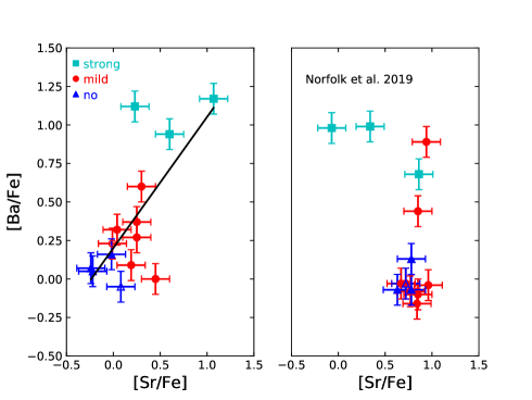
Figure 5: The ([Ba/Fe], [Sr/Fe]) plane from this analysis (left panel) and from N19 (right panel). The left panel reveals that there exists a correlation between the [Sr/Fe] and [Ba/Fe] abundance ratios,

represented by the solid line corresponding to a least-square fit to the data. The ”strong”, ”mild” and ”no” stars (see Sect. 5) are color-coded as indicated in the label. Open symbols refer to stars with a Li abundance determination. The right panel shows [Ba/Fe] and [Sr/Fe] from N19.

Figure 6 reveals as well that ”no-s” stars cannot be attributed to an unrecognized positive luminosity effect on the Sr II lines (i.e., a low gravity $\log g$ causing a strengthening of lines from ionized species), since these ”no-s” stars are not restricted to low $\log g$ values.

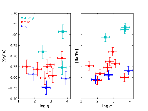
Figure 6: The [Sr/Fe] and [Ba/Fe] abundance ratios vs $\log g$. Symbols are as in Fig. 5.

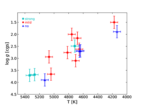
Figure 7: Kiel diagram ($\log g$ vs $T_{\rm eff}$) for the programme stars.

It is worth noting that the two most enriched barium stars are actually barium dwarfs (Figs. 6 and 7). Curiously enough, N19 mention that, because their machine-learning algorithm used a training sample composed of giant stars only, they are therefore ”unable to identify s-process enhanced dwarf stars”. Here we show the contrary, because the 4554 Å  and 4934 Å  Ba II lines are sensitive to a Ba enhancement both in giants and dwarfs (in Fig. 4, HIP 69788 and TYC 3423-696-1 are dwarfs whereas TYC  4837-925-1 is a giant). Therefore, the residuals between the observed flux at those wavelengths and the Cannon data-driven model will be able to identify barium stars, irrespective of them being dwarfs or giants.

6 Discussion of individual stars

BD $\mathbf{-07^{\circ}402}$: This object is the only mild Ba star with a measurable Li abundance of $\log\epsilon_{\rm Li}=1.3$ dex, just large enough to qualify it as a Li-rich K giant (Jorissen et al., 2020).
BD $\mathbf{+44^{\circ}575}$: This mild Ba star presents strong enrichments in Na and Mg.
HD 7863: This ”no-s” star is one of four objects in our sample that exhibits a larger than average N abundance ([N/Fe] $\geq 0.7$; Fig. 12 and Sect. 4.2).
HIP 69788: This star has atmospheric parameters which differ the most between our study and that of N19 (see Table 1 and Sect. 8).
TYC 22$-$155$-$1: This star exhibits a strong enrichment in Mg.
TYC 2913$-$1375$-$1: For this star, an accurate Sr abundance could not be derived, since the Sr I lines are weak and the spectrum is too noisy in the violet to access the Sr II lines. Nevertheless, Zr, Ba, and La lines reveal that this star has mild s-process enhancements.
TYC 3144$-$1906$-$1: This is the second object with a measured Li abundance, but not large enough though ($\log\epsilon_{\rm Li}=0.6$ dex) to be considered as a Li-rich K giant. While it is not enriched in any s-process elements, this star shows a high enhancement in N ([N/Fe] = 1.40 dex; Fig. 12).
TYC 4684$-$2242$-$1: Another ”no-s” star with a larger than average N abundance (Fig. 12). It is worth noting that 3 out the 4 N-rich stars ([N/Fe] $\geq 0.7$) do not show any s-process enhancement.

7 Origin of the peculiarities of mild and strong barium stars

7.1 Binary frequency

According to the canonical scenario (McClure, 1983; Jorissen et al., 2019; Escorza et al., 2019), barium stars form in a binary system. Table 4 therefore collects the kinematical properties of our programme stars. Contrary to what is announced in their paper, N19 do not provide the LAMOST radial velocities (RVs) in their supplementary material. Therefore, we resorted to Gaia Data Release 2 (GDR2; Katz et al., 2019) to get one RV value to compare to the HERMES value. GDR2 velocities refer to epoch 2015.5 (JD 2457205), whereas HERMES RVs were taken roughly 1700 d later, offering a large enough time span to efficiently detect even long-period binaries.

The uncertainty $\epsilon$ (listed in Table 4) on the GDR2 RVs has been computed from $G_{\rm RVS}$ (the Gaia magnitude in the RVS band) along the same method as discussed by Jorissen et al. (2020, their Eqs. 3 and 4), except that Eq. (4) has been replaced by one depending on the Tycho $B_{T}-V_{T}$ color index, as listed in Table 7 of Jordi (2018). As can be seen in Table 4, uncertainties on the GDR2 RVs are on the order of 0.3 km s^-1 for the brightest targets ($G_{\rm RVS}\sim 8$) and go up to 1 km s^-1 for the faintest objects ($G_{\rm RVS}\sim 10.8$). We note that most of the stars have the computed $\epsilon$ uncertainty is very similar to the RV uncertainty listed by GDR2 (except for the binary HIP 69788). Based on the above, we have flagged as binaries all stars with $\Delta RV\geq 3\;\epsilon$.

As expected, 2 out of 3 strong barium stars show a clear binary signature, and the third one (TYC 591$-$1090$-$1) is the faintest in the sample, and despite its large $\Delta RV$ value of 1.55 km s^-1, it does not fulfill the $3\epsilon$ condition. The results for the other classes are intriguing, since only one of the 7 mild barium stars diagnosed exhibit statistically-significant RV variations, and on the opposite, 2 out of the 4 ’no-s’ stars show a binary signature.

We see no obvious explanation for the high prevalence of binaries among the latter category, other than small-number fluctuations. Concerning the mild Ba stars, it is still possible that their RV variations are more difficult to detect since they contain a larger proportion of binaries with very long periods ($>5000$ d) than strong barium stars do (see Fig. 7 of Jorissen et al., 2019), thus explaining the lower apparent frequency of binary signatures among mild barium stars. Alternatively, some mild barium stars with no binary signature might represent the upper tail of the [Ba/Fe] range in the Galactic ([Ba/Fe], [Fe/H]) trend (Edvardsson et al., 1993). Such mild barium stars are especially present at metallicities in the range $[-0.4\;+0.1]$ dex (Fig. 15 panel $k$ of Edvardsson et al. 1993, Fig. 5 of Tautvaišienė et al. 2021).

All non-binary mild barium stars but TYC 2913-1375-1 have [Fe/H] in the above range, making it likely that they owe their mild-barium nature to the fluctuations in the Galactic chemical evolution. Figure 8, which displays the Toomre diagram of the programme stars, reveals no difference in their kinematic properties, they all belong to the Galactic thin disc.

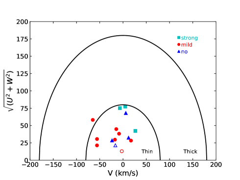
Figure 8: Toomre diagram of the programme stars, with the black line delineating the location of thin-disk stars (as in Fig. 4 of N19).

Table 4: Kinematic properties of the programme stars.

Name	$JD$	RV	$\Delta RV$	$\epsilon$	$G_{\rm RVS}$	source	$U$	$V$	$W$	Gaia DR2	Bin./Rem.
	(-2400000)	(km s${}^{-1})$	(km s${}^{-1})$	(km s${}^{-1})$			(km s${}^{-1})$	(km s${}^{-1})$	(km s${}^{-1})$
no s-process enrichment
HD 7863	57205	$-27.82\pm 0.34$	0.45	0.29	8.09	GDR2	24.95	-23.58	-13.81	397523176280439808	n
	58882.41	$-28.27\pm 0.07$				HER
HIP 69788	57205	$6.56\pm 1.94$	55.93	0.42	9.39	GDR2	31.08	11.94	-9.27	3667671452515762944	y
	58877.70	$-49.37\pm 0.07$				HER
TYC 3144$-$1906$-$1	57205	$-21.56\pm 0.33$	1.06	0.28	7.84	GDR2	-20.73	-16.47	-5.61	2077143186195922176	y
	59090.45	$-22.62\pm 0.07$				HER
TYC 4684$-$2242$-$1	57205	$36.53\pm 0.44$	0.92	0.41	9.35	GDR2	-66.36	6.01	-15.01	2478965826587133568	n
	58882.33	$35.61\pm 0.07$				HER
mild s-process enrichment
BD $-07^{\circ}$ 402	57205	$-12.96\pm 0.17$	0.48	0.29	8.04	GDR2	4.72	-2.66	12.05	2486894817251498240	n
	58882.37	$-13.44\pm 0.07$				HER
BD $+44^{\circ}$ 575	57205	$-12.61\pm 0.26$	0.50	0.28	7.78	GDR2	28.21	17.09	1.94	340768207120632832	n
	58878.41	$-13.11\pm 0.07$				HER
TYC 22$-$155$-$1	57205	$-37.70\pm 0.58$	0.35	0.33	8.71	GDR2	-48.38	-65.05	32.26	2539172197106047872	n
	58882.36	$-38.05\pm 0.07$				HER
TYC 2913$-$1375$-$1	57205	$-2.89\pm 0.42$	0.15	0.48	9.70	GDR2	2.22	-14.52	44.81	193703372946249216	n
	59090.71	$-3.04\pm 0.07$				HER
TYC 3305$-$571$-$1	57205	$-57.93\pm 0.33$	0.52	0.37	9.08	GDR2	30.31	-55.92	3.80	437946515118550016	n
	58878.48	$-58.45\pm 0.07$				HER
TYC 4837$-$925$-$1	57205	$-22.91\pm 0.23$	0.52	0.37	9.11	GDR2	35.55	-8.52	-13.98	3081162263449705984	n
	58877.55	$-23.43\pm 0.07$				HER
TYC 3423$-$696$-$1	57205	$5.37\pm 0.21$	$-3.16$	0.40	9.26	GDR2	-21.20	-55.96	-2.78	1016739606459940608	y
	58877.61	$8.53\pm 0.07$				HER
TYC 752$-$1944$-$1	58877.49	$19.04\pm 0.07$	-			HER	4.66	-17.38	-29.26	3157928756551254400	?
strong s-process enrichment
TYC 2250$-$1047$-$1	57205	$19.39\pm 0.75$	3.44	0.75	10.41	GDR2	-76.78	4.84	-9.30	2839977000550809856	y
	59090.61	$15.95\pm 0.07$				HER
TYC 2955$-$408$-$1	57205	$41.15\pm 0.56$	2.07	0.42	9.41	GDR2	-61.94	-6.77	-42.54	953203601197511808	y
	58879.54	$39.08\pm 0.07$				HER
TYC 591$-$1090$-$1	57205	$8.80\pm 0.88$	1.55	1.00	10.83	GDR2	41.23	26.56	9.10	2757528128276067840	n
	59090.64	$7.25\pm 0.07$				HER

7.2 Location in the HRD

Figure 9 presents the location of our programme stars in the Hertzsprung-Russell diagram (HRD). In this plot, we used the spectroscopic $T_{\rm eff}$ values listed in Table 1 and determined the luminosity of each target by combining the flux obtained from integrating their spectral energy distributions (SED) with the distances computed by Bailer-Jones et al. (2021) from the Gaia Early Data Release 3 parallaxes (Gaia Collaboration et al., 2020). To build and fit the SEDs, we applied the methodology described by Escorza et al. (2017) and successfully used in combination with spectroscopic parameters. The tool performs a $\chi^{2}$-grid-search to find the best-fitting MARCS model atmosphere (Gustafsson et al., 2008) to the available broadband photometry for each target collected from the SIMBAD database (Wenger et al., 2000), treating the total line-of-sight reddening $E_{B-V}$ as a free parameter for which we optimise. We used the parameter ranges obtained from the spectroscopic analysis to limit $T_{\rm eff}$ and $\log g$, and we fixed the metallicity to the closest available in the MARCS grid ($0.0,-0.25$ or $-0.5$ for our targets), leaving $E_{B-V}$ as the only fully unconstrained parameter. Then each best-fitting SED model is corrected for interstellar extinction assuming that the line-of-sight extinction $A_{V}$ follows the Galactic extinction law given by $A_{V}=R_{V}\times E_{B-V}$ with $R_{V}=3.1$ (Fitzpatrick, 1999). The SED is then integrated to get the total flux.

The star locations in the HRD are compared with evolutionary tracks from STAREVOL (Siess & Arnould, 2008) for three metallicities, [Fe/H] = $-0.5,-0.25$, and 0. A correlation may seem to exist between mass and metallicity: at the lowest metallicity [Fe/H]$=-0.5$ (panel a of Fig. 9), barium stars are found in the full mass range 1.2 - 3 M_⊙, whereas at solar metallicity (panel c of Fig. 9), they are restricted to the much narrower range 0.9 – 1.5 M_⊙. This correlation is not confirmed, however, by the larger sample studied by Jorissen et al. (2019, their Fig.  17). Thus the segregation observed in Fig. 9 is likely the result of small-sample statistics.

To summarize, the confirmed barium stars from N19 are found in the mass range 0.9 – 3 M_⊙ and are located all the way from the end of the main-sequence till the red clump through the red-giant phase.

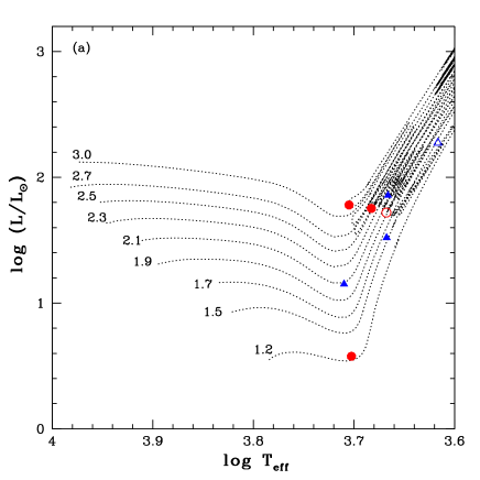
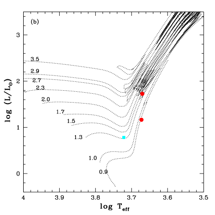
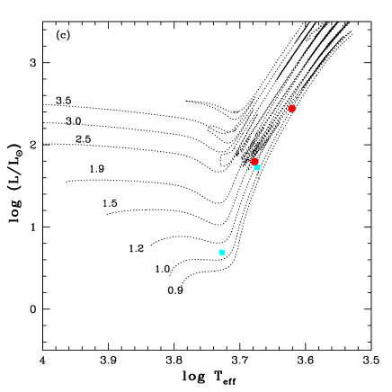
Figure 9: Location of barium stars in the HRD compared with STAREVOL tracks: (a) [Fe/H] = 0 (b) [Fe/H] $=-0.25$ (c) [Fe/H] $=-0.5$. Symbols are as in Fig. 3

7.3 Abundance trends

In most of the barium stars studied here, the second s-process peak reaches slightly larger overabundance levels than the first peak, resulting in [hs/ls] ratios ranging from 0 to 0.5 dex (left panel of Fig. 10), with only two exceptions (TYC 3423-696-1 and TYC 2955-408-1) where [hs/ls] $=-0.1$. As usual in barium stars, the [hs/ls] ratio does not show a strong correlation with metallicity (right panel of Fig.  10).

The distribution of [La/Fe] vs [Fe/H] (right panel of Fig. 11) indicates that there might be a weak correlation between metallicity and the level of s-process enrichment, since strong barium stars with [La/Fe] $\geq 0.75$ have [Fe/H] $\leq-0.30$ whereas mild barium stars cluster instead around a slightly subsolar metallicity ([Fe/H] $\sim-0.1$).

As explained in Sect. 4.3, ’no-s’ stars show comparatively large enhancements in N and hence low [C/N] values (Fig. 12). The low [C/N] values in these stars may be the result of an efficient mixing as they ascend the first giant branch (RGB), since their [N/Fe] ratio increases with luminosity along the RGB.

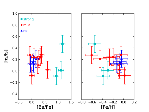
Figure 10: The [hs/ls] ratio as a function of various abundance ratios.

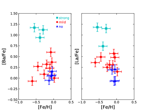
Figure 11: The [Ba/Fe] and [La/Fe] ratios as a function of metallicity [Fe/H].

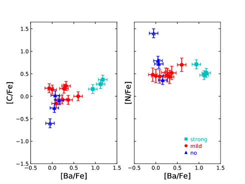
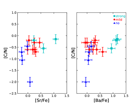
Figure 12: Various diagnostics involving C and N.

8 Automatic vs. manual classification

Table 1 reveals that 4 stars out of 15 have in fact been erroneously flagged as mild barium stars by the machine-learning method used by N19. The topic of this section is to identify what may be learned about the power of such machine-learning methods: can we identify why machine-learning led to such a large fraction of ”false positives”? What are the properties of these false positives, with respect to either the accuracy of the atmospheric parameters delivered by ”The Cannon” or the properties of the Ba and Sr lines used (are they saturated or not?)?

Table 1 compares the atmospheric parameters obtained by N19 and by our high-resolution abundance study. Effective temperatures and gravities are generally in good agreement (the worst discrepancy is 200 K for $T_{\rm eff}$ in HIP 69788 and TYC 2250–1047–1, and 1 dex for the gravity of HIP 69788). The metallicities are more discrepant, up to 0.3 dex (HIP 69788, BD +44^∘575, and TYC 4837$-$925$-$1). However, these discrepant atmospheric parameters are not restricted to those cases where we found no s-process enrichments. Therefore, we believe that false positives do not result from possible inaccuracies in the machine-learning atmospheric parameters.

N19 used strong Sr II and Ba II lines to derive Sr and Ba abundances. From the Sr II lines at 4077 and 4215 Å , N19 found [Sr/Fe] values in the range 0.8 – 1.0 dex for the four stars with no s-process enrichment in our analysis. Figure 1 reveals that the Sr II line at 4215 Å  used by N19 is not only saturated, but also blended by the CN band with its band head at 4216 Å. When this band is strong (i.e., in K giants with a large N abundance [N/Fe] $\geq 0.7$), it likely causes false ”Sr-only” positives.

9 Conclusions

A detailed abundance analysis of fifteen suspected Ba stars from N19 has been carried out. It was found that three of them are strongly enhanced with s-process elements, eight are mildly enhanced and the remaining four show no enhancement in s-process elements. The machine-learning technique used earlier by N19 on low-resolution LAMOST spectra classified thirteen among these fifteen stars as Sr-only candidates. Instead, our traditional approach based on an individual spectroscopic analysis of high-resolution spectra revealed that four of these 13 stars do not have significant overabundances of any s-process elements. We investigated the possible reasons for the high incidence of the Sr-abundance tag obtained by the machine-learning technique. We found that the Sr lines used by N19 are generally saturated, thus leading to spurious overabundances. Neither has the possibility of a nitrogen enhancement in these stars, as revealed by our analysis, been considered by the N19 analysis. Because of the blend between the Sr II 4215.5 Å  line and the CN band head, a high N abundance, if overlooked, may lead to spurious Sr overabundances.

We spectroscopically identified two strong Ba dwarfs in the sample, further confirmed by their location in the HR diagram. We found significant radial velocity variations in five objects, two in the strong Ba class, one in the mild Ba class, and more surprisingly, two in the no-s class. All the sample stars have Galactic thin-disk kinematic signatures, as evident from their location in the Toomre diagram.

We also compared the properties of mild and strong Ba stars. Various heavy-s abundances revealed a sensitivity to metallicity, since all strong Ba stars have sub-solar metallicities. Carbon and N abundances seem to behave differently in the two groups, with non-Ba stars having a tendency to be C-poor but N-rich.

Appendix A Abundances

The following tables present the elemental abundances of the programme stars. NLTE abundance corrections are applied when available, i.e. for O and Sr. We used the same atomic and molecular lines presented in Karinkuzhi et al. (2018, 2021).

Table 5: Light element abundances.

Star Name	[Ca/Fe]	[Sc/Fe]	[Ti/Fe]	[V/Fe]	[Cr/Fe]	[Ni/Fe]	[Cu/Fe]	[Zn/Fe]
HD 7863	0.03	–	0.12	0.44	0.03	$-$0.30	$-$0.22	$-$0.49
HIP 69788	0.30	–0.01	0.09	–0.26	0.40	$-$0.03	0.15	0.03
TYC 3144$-$1906$-$1	$-$0.21	-0.02	–0.12	0.08	0.09	$-$0.24	$-$0.06	$-$0.43
TYC 4684$-$2242$-$1	0.26	0.05	0.25	0.47	0.21	$-$0.07	0.11	$-$0.11
BD$-$07 402	0.07	0.11	0.16	0.38	0.11	$-$0.01	0.07	0.05
BD+44 575	0.41	0.15	0.50	–	0.41	0.01	0.01	$-$0.31
TYC 22$-$155$-$1	0.36	–	0.40	0.47	0.16	0.13	0.21	0.24
TYC 2913$-$1375$-$1	0.27	0.06	0.01	0.06	0.57	0.39	0.11	0.08
TYC 3305$-$571$-$1	0.31	0.20	0.10	0.05	0.10	$-$0.17	0.21	0.09
TYC 752$-$1944$-$1	0.04	–	$-$0.17	0.05	0.14	0.01	-0.11	0.02
TYC 4837$-$925$-$1	0.03	0.22	0.17	0.19	0.28	0.05	$-$0.02	-0.04
TYC 3423$-$696$-$1	0.24	–	0.23	0.45	–	$-$0.24	0.09	$-$0.03
TYC 2250$-$1047$-$1	0.21	0.20	0.20	0.30	0.31	0.03	$-$0.24	0.19
TYC 2955$-$408$-$1	0.35	–	0.24	–	0.35	–	0.20	0.43
TYC 591$-$1090$-$1	0.21	0.15	0.20	0.10	0.36	$-$0.22	0.11	$-$0.26

Table 2: Elemental abundances

		BD $-07^{\circ}402$					BD $+44^{\circ}575$				HD 7863
	Z	log${}_{\odot}{\epsilon}^{a}$	log${\epsilon}$	$\sigma_{l}$ (N)	[X/Fe] $\pm\leavevmode\nobreak\ \sigma_{t}$		log${\epsilon}$	$\sigma_{l}$(N)	[X/Fe] $\pm\leavevmode\nobreak\ \sigma_{t}$		log${\epsilon}$	$\sigma_{l}$(N)	[X/Fe] $\pm\leavevmode\nobreak\ \sigma_{t}$
Li	3	1.05	1.30	0.1(1)	0.36 $\pm$ 0.18		–	–	–		–	–	–
C	6	8.43	8.25	0.1(4)	$-$0.07 $\pm$ 0.11		8.15	0.10(4)	0.17 $\pm$ 0.11		8.10	0.10(1)	$-$0.26 $\pm$ 0.13
12C/13C	–	–	–	–	19		–	–	13		–	–	19
N	7	7.83	8.25	0.1(10)	0.53 $\pm$ 0.06		7.85	0.05(15)	0.47 $\pm$ 0.05		8.55	0.02(12)	0.79 $\pm$ 0.05
O	8	8.69	8.8	0.1(1)	0.22 $\pm$ 0.12		8.60	0.10(1)	0.36 $\pm$ 0.13		8.65	0.10(1)	0.03 $\pm$ 0.12
Na	11	6.24	6.53	0.08(2)	0.40 $\pm$ 0.12		6.38	0.08(2)	0.59 $\pm$ 0.12		6.44	0.11(4)	0.27 $\pm$ 0.12
Mg	12	7.60	–	–	–		8.10:	0.10(2)	0.90 $\pm$ 0.15		7.44	0.10(3)	$-$0.09 $\pm$ 0.15
Rb	37	2.52	2.50	0.10(2)	0.09 $\pm$ 0.16		–	–	–		2.30	0.10(2)	$-$0.15 $\pm$ 0.16
Sr	38	2.87	2.75	0.16(3)	$-$0.01 $\pm$ 0.13		2.67	0.00(2)	0.25 $\pm$ 0.11		2.58	0.10(3)	$-$0.22 $\pm$ 0.10
Y	39	2.21	2.09	0.14(7)	$-$0.01 $\pm$ 0.14		1.72	0.04(6)	$-$0.04 $\pm$ 0.13		1.76	0.20(9)	$-$0.38 $\pm$ 0.14
Zr	40	2.58	2.75	0.07(3)	0.28 $\pm$ 0.13		2.61	0.04(4)	0.48 $\pm$ 0.12		2.50	0.10(2)	$-$0.15 $\pm$ 0.14
Nb	41	1.46	–	–	–		1.48	0.12(3)	0.47 $\pm$ 0.15		–	–	-
Ba	56	2.18	2.30	0.1(2)	0.23 $\pm$ 0.07		2.00	0.10(1)	0.27 $\pm$ 0.10		2.15	0.15(4)	0.05 $\pm$ 0.08
La	57	1.10	1.30	0.10(6)	0.31 $\pm$ 0.10		1.14	0.05(8)	0.49 $\pm$ 0.09		0.96	0.06(4)	$-$0.07 $\pm$ 0.10
Ce	58	1.58	1.64	0.08(6)	0.17 $\pm$ 0.07		1.50	0.10(4)	0.37 $\pm$ 0.08		1.34	0.12(7)	$-$0.14 $\pm$ 0.07
		HIP 69788					TYC 22$-$155$-$1				TYC 2250$-$1047$-$1
	Z	log${}_{\odot}{\epsilon}^{a}$	log${\epsilon}$	$\sigma_{l}$(N)	[X/Fe] $\pm\leavevmode\nobreak\ \sigma_{t}$		log${\epsilon}$	$\sigma_{l}$(N)	[X/Fe] $\pm\leavevmode\nobreak\ \sigma_{t}$		log${\epsilon}$	$\sigma_{l}$(N)	[X/Fe] $\pm\leavevmode\nobreak\ \sigma_{t}$
C	6	8.43	8.30	0.10(4)	$-$0.09 $\pm$ 0.11		8.45	0.10(4)	0.23 $\pm$ 0.11		8.25	0.10(4)	0.37 $\pm$ 0.11
N	7	7.83	8.15	0.05(15)	0.36 $\pm$ 0.05		8.05	0.10(9)	0.43 $\pm$ 0.06		7.80	0.10(10)	0.52 $\pm$ 0.06
O	8	8.69	8.90	0.10(2)	0.25 $\pm$ 0.10		8.90	0.10(1)	0.44 $\pm$ 0.13		8.60	0.10(1)	0.46 $\pm$ 0.13
Na	11	6.24	6.30	0.10(2)	0.10 $\pm$ 0.13		6.35	0.05(2)	0.31 $\pm$ 0.11		5.85	0.10(2)	0.16 $\pm$ 0.13
Mg	12	7.60	–	–	–		8.60:	0.10(1)	1.20 $\pm$ 0.15		–	–	–
Rb	37	2.52	2.50	0.10(2)	0.02 $\pm$ 0.16		–	–	–		2.10	0.10(1)	0.13 $\pm$ 0.17
Sr	38	2.87	2.81	0.16(2)	$-$0.02 $\pm$ 0.15		2.71	0.19(3)	0.04 $\pm$ 0.14		3.39	0.19(2)	1.07 $\pm$ 0.16
Y	39	2.21	1.79	0.09(5)	$-$0.38 $\pm$ 0.13		1.78	0.06(4)	$-$0.23 $\pm$ 0.13		2.10	0.13(5)	0.44 $\pm$ 0.14
Zr	40	2.58	2.20	0.10(3)	$-$0.34 $\pm$ 0.13		2.55	0.05(4)	0.17 $\pm$ 0.12		2.80	0.10(2)	0.77 $\pm$ 0.14
Ba	56	2.18	2.30	0.10(1)	0.16 $\pm$ 0.10		2.30	0.10(2)	0.32 $\pm$ 0.07		2.80	0.10(3)	1.17 $\pm$ 0.07
La	57	1.10	1.00	0.10(4)	$-$0.06 $\pm$ 0.11		1.21	0.12(9)	0.31 $\pm$ 0.10		1.73	0.11(8)	1.18 $\pm$ 0.10
Ce	58	1.58	1.30	0.10(2)	$-$0.24 $\pm$ 0.09		1.50	0.10(2)	0.12 $\pm$ 0.09		2.00	0.07(4)	0.97 $\pm$ 0.07

^a Asplund et al. (2009)
$:$ Uncertain abundances due to noisy/blended region

Table 2: Elemental abundances

		TYC 2913$-$1375$-$1					TYC 2955$-$408$-$1				TYC 3144$-$1906$-$1
	Z	log${}_{\odot}{\epsilon}^{a}$	log${\epsilon}$	$\sigma_{l}$ (N)	[X/Fe] $\pm\leavevmode\nobreak\ \sigma_{t}$		log${\epsilon}$	$\sigma_{l}$(N)	[X/Fe] $\pm\leavevmode\nobreak\ \sigma_{t}$		log${\epsilon}$	$\sigma_{l}$(N)	[X/Fe] $\pm\leavevmode\nobreak\ \sigma_{t}$
Li	3	1.05	–	–	–		–	–	–		0.60	0.10(1)	$-$0.32 $\pm$ 0.18
C	6	8.43	8.00	0.10(3)	0.18 $\pm$ 0.11		8.2	0.10(4)	0.16 $\pm$ 0.11		7.70	0.10(1)	$-$0.60 $\pm$ 0.14
N	7	7.83	7.70	0.10(10)	0.48 $\pm$ 0.06		8.15	0.06(15)	0.71 $\pm$ 0.05		9.10		1.40 $\pm$ 0.11
O	8	8.69	–	–	–		8.60	0.10(1)	0.33 $\pm$ 0.13		–	–	–
Na	11	6.24	8.60	0.10(1)	0.52 $\pm$ 0.15		6.15	0.10(2)	0.30 $\pm$ 0.13		6.60	0.10(2)	0.49 $\pm$ 0.13
Mg	12	7.60	–	–			8.20	0.10(3)	0.99 $\pm$ 0.15		–	–	–
Rb	37	2.52	–	–	–		2.48	0.08(2)	0.35 $\pm$ 0.15		2.48	0.08(2)	0.09 $\pm$ 0.16
Sr	38	2.87	–	–	–		3.08	0.19(2)	0.60 $\pm$ 0.16		2.82	0.05(2)	0.08 $\pm$ 0.15
Y	39	2.21	1.25	0.21(5)	$-$0.35 $\pm$ 0.16		2.43	0.13(9)	0.61 $\pm$ 0.14		1.88	0.25(5)	$-$0.20 $\pm$ 0.17
Zr	40	2.58	2.28	0.04(4)	0.31 $\pm$ 0.12		3.15	0.12(3)	0.96 $\pm$ 0.14		2.67	0.11(6)	0.22 $\pm$ 0.13
Nb	41	1.46	–	–	–		1.98	0.06(4)	0.95 $\pm$ 0.15		–	–	–
Ba	56	2.18	1.50	0.14(2)	$-$0.07 $\pm$ 0.10		2.73	0.05(3)	0.94 $\pm$ 0.05		2.00	0.10(2)	$-$0.05 $\pm$ 0.07
La	57	1.10	0.85	0.14(7)	0.36 $\pm$ 0.11		1.45	0.07(9)	0.74 $\pm$ 0.10		1.16	0.16(10)	0.19 $\pm$ 0.11
Ce	58	1.58	1.12	0.11(5)	0.15 $\pm$ 0.07		1.84	0.09(8)	0.65 $\pm$ 0.07		1.53	0.05(4)	0.08 $\pm$ 0.06
		TYC 3305$-$571$-$1					TYC 3423$-$6966$-$1				TYC 4684$-$2242$-$1
	Z	log${}_{\odot}{\epsilon}^{a}$	log${\epsilon}$	$\sigma_{l}$(N)	[X/Fe] $\pm\leavevmode\nobreak\ \sigma_{t}$		log${\epsilon}$	$\sigma_{l}$(N)	[X/Fe] $\pm\leavevmode\nobreak\ \sigma_{t}$		log${\epsilon}$	$\sigma_{l}$(N)	[X/Fe] $\pm\leavevmode\nobreak\ \sigma_{t}$
C	6	8.43	8.30	0.10(4)	$-$0.08 $\pm$ 0.11		8.60	0.10(3)	0.15 $\pm$ 0.12		8.40	0.10(4)	0.02 $\pm$ 0.11
N	7	7.83	8.30	0.10(10)	0.52 $\pm$ 0.07		8.30	0.15(15)	0.45 $\pm$ 0.06		8.50	0.06(15)	0.72 $\pm$ 0.05
O	8	8.69	8.90	0.10(1)	0.29 $\pm$ 0.13		8.90	0.10(1)	0.22 $\pm$ 0.12		8.90	0.10(1)	0.26 $\pm$ 0.12
Na	11	6.24	6.53	0.08(2)	0.34 $\pm$ 0.12		6.60	0.10(2)	0.34 $\pm$ 0.13		6.60	0.10(2)	0.41 $\pm$ 0.13
Mg	12	7.60	–	–	–		–	–	–		8.20:	0.10(1)	0.65 $\pm$ 0.15
Rb	37	2.52	2.55	0.10(2)	0.08 $\pm$ 0.16		2.80	0.10(2)	0.26 $\pm$ 0.16		2.60	0.10(1)	0.13 $\pm$ 0.17
Sr	38	2.87	3.05	0.10(2)	0.25 $\pm$ 0.12		3.34	0.06(2)	0.45 $\pm$ 0.10		2.58	0.28(2)	$-$0.24 $\pm$ 0.22
Y	39	2.21	2.18	0.14(8)	0.02 $\pm$ 0.14		2.36	0.19(7)	0.13 $\pm$ 0.15		2.04	0.14(8)	$-$0.12 $\pm$ 0.14
Zr	40	2.58	2.78	0.02(3)	0.25 $\pm$ 0.12		2.80	0.10(3)	0.20 $\pm$ 0.14		2.75	0.05(4)	0.22 $\pm$ 0.12
Nb	41	1.46	–	–	–		–	–			1.80:	0.10(1)	0.39 $\pm$ 0.15
Ba	56	2.18	2.50	0.10(2)	0.37 $\pm$ 0.08		2.20	0.10(1)	0.00 $\pm$ 0.11		2.20	0.10(2)	0.07 $\pm$ 0.07
La	57	1.10	1.53	0.04(8)	0.48 $\pm$ 0.10		1.27	0.12(5)	0.15 $\pm$ 0.11		1.26	0.04(5)	0.21 $\pm$ 0.10
Ce	58	1.58	1.88	0.15(5)	0.35 $\pm$ 0.10		1.77	0.05(3)	0.02 $\pm$ 0.06		1.67	0.11(6)	0.14 $\pm$ 0.07
		TYC 4837$-$925$-$1					TYC 591$-$1090$-$1				TYC 752$-$1944$-$1
	Z	log${}_{\odot}{\epsilon}^{a}$	log${\epsilon}$	$\sigma_{l}$ (N)	[X/Fe] $\pm\leavevmode\nobreak\ \sigma_{t}$		log${\epsilon}$	$\sigma_{l}$(N)	[X/Fe] $\pm\leavevmode\nobreak\ \sigma_{t}$		log${\epsilon}$	$\sigma_{l}$(N)	[X/Fe] $\pm\leavevmode\nobreak\ \sigma_{t}$
C	6	8.43	8.00	0.10(4)	$-$0.16 $\pm$ 0.11		8.40	0.10(4)	0.27 $\pm$ 0.11		8.35	0.05(4)	0.00 $\pm$ 0.10
N	7	7.83	8.00	0.10(15)	0.44 $\pm$ 0.06		8.15	0.15(15)	0.47 $\pm$ 0.07		8.45	0.05(15)	0.70 $\pm$ 0.05
O	8	8.69	8.60	0.10(1)	0.18 $\pm$ 0.12		8.40	0.20(2)	0.01 $\pm$ 0.16		8.75	0.10(1)	0.17 $\pm$ 0.12
Na	11	6.24	6.25	0.05(2)	0.28 $\pm$ 0.11		6.05	0.05(2)	0.11 $\pm$ 0.11		6.45	0.10(2)	0.28 $\pm$ 0.13
Mg	12	7.60	–	–	–		–	–	–		7.75	0.15(2)	0.23 $\pm$ 0.15
Rb	37	2.52	–	–	–		–	–	–		2.80	0.10(1)	0.28 $\pm$ 0.17
Sr	38	2.87	2.79	0.18(2)	0.19 $\pm$ 0.16		2.80	0.10(1)	0.23 $\pm$ 0.13		3.09	0.18(1)	0.30 $\pm$ 0.12
Y	39	2.21	1.74	0.12(6)	$-$0.20 $\pm$ 0.14		3.03	0.04(9)	1.12 $\pm$ 0.13		2.60	0.10(5)	0.47 $\pm$ 0.14
Zr	40	2.58	2.48	0.02(3)	0.17 $\pm$ 0.16		3.37	0.07(5)	1.09 $\pm$ 0.12		3.09	0.02(4)	0.59 $\pm$ 0.12
Ba	56	2.18	2.00	0.10(2)	0.09 $\pm$ 0.07		3.00	0.15(2)	1.12 $\pm$ 0.11		2.70	0.10(1)	0.60 $\pm$ 0.10
La	57	1.10	1.08	0.04(6)	0.25 $\pm$ 0.09		1.95	0.14(8)	1.15 $\pm$ 0.11		1.59	0.11(5)	0.57 $\pm$ 0.11
Ce	58	1.58	1.50	0.10(5)	0.19 $\pm$ 0.07		2.36	0.16(4)	1.08 $\pm$ 0.10		2.03	0.06(7)	0.53 $\pm$ 0.06

^a Asplund et al. (2009)
$:$ Uncertain abundances due to noisy/blended region