Flood Segmentation on Sentinel-1 SAR Imagery with Semi-Supervised Learning

Abstract

Floods wreak havoc throughout the world, causing billions of dollars in damages, and uprooting communities, ecosystems and economies. The NASA Impact Flood Detection competition tasked participants with predicting flooded pixels after training with synthetic aperture radar (SAR) images in a supervised setting. We propose a semi-supervised learning pseudo-labeling scheme that derives confidence estimates from U-Net ensembles, progressively improving accuracy. Concretely, we use a cyclical approach involving multiple stages (1) training an ensemble model of multiple U-Net architectures with the provided high confidence hand-labeled data and, generated pseudo labels or low confidence labels on the entire unlabeled test dataset, and then, (2) filter out quality generated labels and, (3) combine the generated labels with the previously available high confidence hand-labeled dataset. This assimilated dataset is used for the next round of training ensemble models and the cyclical process is repeated until the performance improvement plateaus. We post process our results with Conditional Random Fields. Our approach sets a new state-of-the-art on the Sentinel-1 dataset with 0.7654 IoU, an impressive improvement over the 0.60 IoU baseline. Our method, which we release with all the code and models, can also be used as an open science benchmark for the Sentinel-1 dataset.

1 Introduction

Flooding events are on the rise due to climate change [35], increasing sea levels and increasing extreme weather events, resulting in 10 billion dollars worth of damages annually. Scientists and decision makers can use live Earth observations data via satellites like Sentinel-1 to develop real-time response and mitigation tactics and understand flooding events. The Emerging Techniques in Computational Intelligence (ETCI) 2021 competition on Flood Detection provides SAR Sentinel-1 imagery with labeled pixels for a geographic area prior and post flood event. SAR satellites, such as Sentinel-1, see through clouds and at night so can be used everywhere all the time, making its solutions deployable at scale. Participants are tasked with a semantic segmentation task that identifies pixels that are flooded and is evaluated with Intersection over Union metric (IoU).

Improved flood segmentation in real-time results in delineating open water flood areas. Identifying flood levels aids in effective disaster response and mitigation. Combining the flood extent mapping with local topography generates a plan of action with downstream results including predicting the direction of flow of water, redirecting flood waters, organizing resources for distribution etc. Such a system can also recommend a path of least flood levels in real-time that disaster response professionals can potentially adopt.

Feature based machine learning techniques are also prominent [27] but are intractable as human annotators and featurizers cannot scale. Manual annotation in real time can easily exceed $62,500 daily, and a manual solution quickly becomes intractable. Motivated by prior art [44, 45, 7, 19], we look at semi-supervised techniques, that assume predicted labels with maximally predicted probability as ground truth, and we apply it to flood segmentation. Similar to [19, 3], we treat pseudo labels as an entropy regularizer which eventually outperforms other conventional methods with a small subset of labeled data. For real time deployment we benchmark our solution similar to [23, 36], both of which utilize datasets like WorldFloods or multispectral datasets to enable flood detection, but require large scale manual annotation. Contrary to both, our work with semi supervision reduces the human-in-the-loop load and allows us to take advantage of large unannotated examples in a simple manner. Evidence indicates that post processing with Conditional Random Fields (CRF) [17, 9, 2, 42] may yield improved performance especially for semantic segmentation, and, satellite data [12]. Our work follows along similar lines when we post process with CRFs for flood segmentation.

Our contributions are: (1) We propose a semi-supervised learning scheme with pseudo-labeling that derives confidence estimates from U-Net ensembles. With this we establish the new state-of-the-art flood segmenter and to the best of our knowledge we believe this is the first work to try out semi-supervised learning to improve flood segmentation models. (2) We show that our method is scalable through psuedo labels and generalizable through varying data distributions in different geographic locations and thus is inexpensive to deploy scalably. (3) Additionally, we benchmark the inference pipeline and show that it can be performed in real time aiding in real time disaster mitigation efforts. Our approach also includes uncertainty estimation, allowing disaster response teams to understand its reliability and safety. In an effort to promote open science and cross-collaboration we release all our code and models.

2 Data

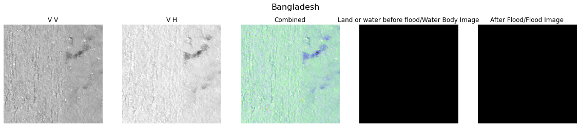
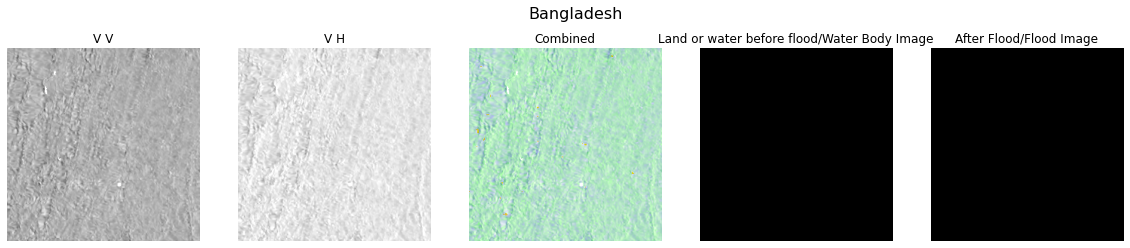
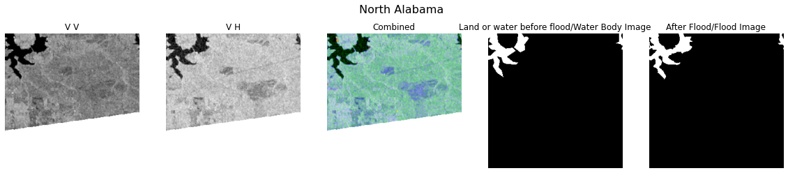
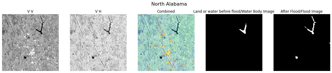
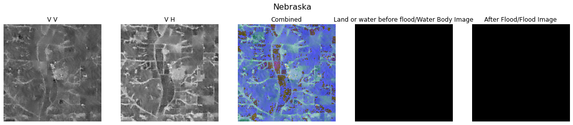
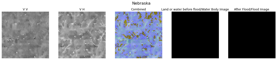
The contest dataset consists of 66k tiled images from various geographic locations. Each RGB training tile is generated VV and VH GeoTIFF files (see raw images in Appendix C, Figure 4) obtained via Hybrid Pluggable Processing Pipeline “hyp3” from the Sentinel-1 C-band SAR imagery. Data also contains swath gaps (see images in Appendix C Figure 5) where less than .5% of an image is present; such images are not used for training. The dataset is imbalanced i.e., the proportion of images with some flood region presence is lower than the images without it, so during training, we ensure each batch contains at least 50% samples having some amount of flood region present through stratified sampling. Flooded water may change in appearance due to added debris and such data can be captured by different sensors, but for our work we do not assume a distinction. The Red River geographic area which is predominant in the test set, is primarily an agricultural hub and recently harvested fields can look similar to floods due to low backscatter in both VV and VH polarizations. Similarly Florence which comprises of the validation set has a primarily urban setting. Such varying backscatter is relevant for performance optimizations and generalizability to test imagery (see combined images in Figure 4), and thus we combine different forms of ensembling with stacking, and, test-time augmentation helping model uncertainty and making the predictions robust. Training augmentation includes horizontal flips, rotations, and elastic transformations, and, test-time augmentations are comprised of Dihedral Group D4 [32].

3 Methodology

We develop a semi-supervised learning scheme with pseudo-labeling that derives confidence estimates from U-Net ensembles motivated from [18]. First, we train an ensemble model of multiple U-Net architectures with the provided high confidence hand-labeled data and, generated pseudo labels or low confidence labels on the entire unlabeled test dataset. We then, filter out quality generated labels and, finally, combine the quality generated labels with the previously provided high confidence hand-labeled dataset. This assimilated dataset is used for the next round of training ensemble models. This cyclical process is repeated until the performance improvement plateaus (see Figure 1). Additionally, we post process our results with Conditional Random Fields (CRF).

Figure 1: Our semi-supervised learning pseudo-labeling scheme that derives confidence estimates from U-Net ensembles with CRFs for post processing.

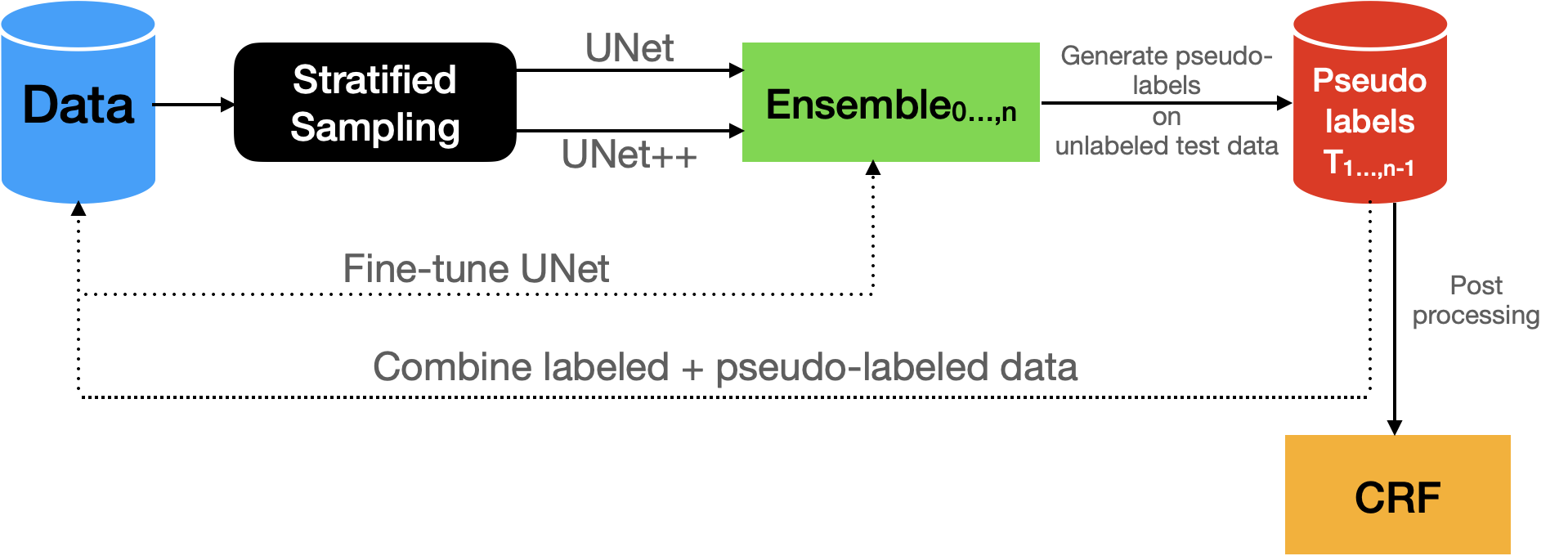
Step 1: Training on available data, performing inference on entire test data, and generating Pseudo Labels.

The provided test data is only from the Red River North region which does not occur in training (Bangladesh + North Alabama + Nebraska) or validation dataset (only Florence), and thus out-of-distribution impacts were imminent. Such differences in distributions prompted us to utilize ensembling. We first train two models with U-Net [30] and U-Net++ [43] both with MobileNetv2 backbones [31] and combined dice and focal loss on the available training data. Both U-Net and U-Net++ share similar inductive biases and we use them to tackle the distribution shifts, owing to different geographic locations and artifacts like recently harvested fields, urban and rural scenarios (see Appendix, Figure 4) etc. Then, create an ensemble with these two trained models.

Step 2: Filtering quality pseudo labels.

Next, we filter over the softmax output of the predictions keeping images where at least 90% of pixels have high confidence of either flood or no flood. In the zeroth training iteration, no pseudo labels are available and training is only on the provided training dataset. For the next step, i.e., step 1 or training iteration 1, pseudo labels from iteration 0 can be used. As such training iteration n can incorporate pseudo labels from step n-1. For standard image classification tasks, it is common to filter the softmaxed predictions with respect to a predefined confidence threshold [38, 33, 46]. In semantic segmentation, we are extending the classification task to a per-pixel case where each pixel of an image needs to be categorized. To filter out the low-confidence predictions, we check if a pre-specified % of the pixel values (in the range of [0, 1]) in each prediction were above a predefined threshold; mathematically denoted in (1).

$$\operatorname{mask}=\left(\sum_{h}\sum_{w}\tilde{Y}>c\right)>p*h*w,$$ (1)

where $\tilde{Y}$ is the prediction vector, $c$ and $p$ denote the confidence and pixel proportion thresholds respectively (both being 0.9 in our case), and $h$ and $w$ are the spatial resolutions of the predicted segmented maps. We compute $\tilde{Y}$ using (2), where $Z$ is the logit vector.

$$\tilde{Y}=max\big{(}softmax(Z,dim=1),dim=1\big{)},$$ (2)

Step 3: Combining Pseudo Labels + Original Training data.

Now, the filtered pseudo labels from the previous stage are incorporated into the training dataset. Thus, a new training dataset is created which is composed of (1) original training data with available ground truth, referred to as “high confidence” labels, and, (2) filtered pseudo labels or “low confidence” labels on the unlabeled test dataset. This assimilated dataset is used for the next round of training individual U-Net, U-Net++ and the ensemble models.

Repeat Steps 1,2,3 and Post processing with CRFs.

With the training data now composed of the original training dataset and pseudo labels from the test dataset, we perform training from scratch of the U-Net and U-Net++ models, and fine-tuning of the U-Net from the previous iteration. Training and fine-tuning are all on the same dataset of original training data and pseudo-labeled test data. Note that the ensemble models are only used to generate predictions, and not for fine-tuning. Now, with three trained models, as before, averaged predictions are generated, and filtered to create the new set of “weak labels”. All the data for training U-Net, U-Net++ and the fine-tuned U-Net is processed through stratified sampling as before. This cyclical process (steps 1,2,3..) are repeated until the performance improvement plateaus, about 20 epochs, post which we perform additional processing with CRFs. Ultimately for each pixel we predict as flooded or not flooded, we also produce confidence intervals that may help disaster response teams understand reliability and safety.

4 Results

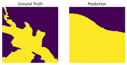
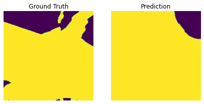
We report all the results obtained from the various approaches in Table 1, and, compare against a random (all zeros to indicate non-flooded pixels, as majority pixels are not flooded) and competition provided baseline (combination of FPN [20] with U-Net). We also provide a few random ground truth comparisons to our predictions in Figure 2. Since the dataset is skewed i.e., majority of pixels are not flooded, we report the IoU for the flooded pixels only. On performing test inference with the U-Net, U-Net++, the ensemble model, and averaged predictions from the ensemble, we note a performance improvement of 2-3% IoU on average for the averaged predictions, in each step. Test-time augmentations on the test data improves our IoU by 5% and further reduces uncertainty. Our results are uniform across all data distribution drifts available in the dataset and initial benchmarks shows that the segmentation masks are generated in approximately 3 seconds for a Sentinel-1 tile that covers an area of approximately 63,152 squared kilometers, larger than the area covered by Lake Huron, the second largest fresh water Great Lake of North America. Our work suggests CRFs are a crucial element for post processing of the predictions as they provide substantial performance improvements.

  

Figure 2: Random selection of Ground Truth comparison against our predictions on the hold-out test set on which the final leaderboard results are presented

Table 1: Leaderboard results for the hold-out test set. Higher IOU ($\uparrow$) is better.

Method Description	IoU $\uparrow$
Random Baseline (all zeroes)	0.00
Competition Provided Baseline	0.60
Standard U-Net	0.57
Ensemble with CRF post processing	0.68
Pseudo labeling + Ensembles with CRF post processing	0.7654

Conclusion

We recognize that it is a privilege to take part in the interdisciplinary research to reduce the impact of flooding events and as such, scaling solutions to deployment is a huge component. We developed a semi-supervised learning pseudo-labeling scheme that derives confidence estimates from U-Net ensembles. We train an ensemble model of multiple U-Net architectures with the provided high confidence hand-labeled data and, generated pseudo labels or low confidence labels on the entire unlabeled test dataset, then, filter out quality generated labels and, finally, combine the quality generated labels with the previously provided high confidence hand-labeled dataset, and, post process our results with CRFs. We show that our method can enable scalable training with data distribution drifts. Additionally, lack of annotated data and scaling while maintaining quality of results is also imperative. Hence our future work involves collaborating with the competition organizers and the UNOSAT team to benchmark real time runtimes and to evaluate the scalability of our solution.

Appendix

Appendix A Implementation Details

Our semi-supervised learning pseudo-labeling scheme that derives confidence estimates from U-Net ensembles involved experimenting with U-Net-inspired architectures [30, 43] and backbones, multiple loss functions like focal loss and dice loss, combining both loss functions into one, and various training and test-time augmentation techniques. We set seeds at various framework and package levels to enable reproducibility, and present results as the average of multiple training runs. For additional experimental configurations, we refer the readers to our code repository on GitHub.

Sampling.

There is an imbalance problem in the training dataset i.e. the number of satellite images that have presence of flood regions is smaller than the number of images that do not have contain flood regions. This is why we follow a stratified sampling strategy during data loading to ensure half of the images in any given batch always contain some flood regions. Empirically we found out that this sampling significantly helped in convergence. Using this sampling strategy in our setup was motivated from a solution that won a prior Kaggle competition [1]. Research in the domain of reducing the impact of swath gaps [11] also exists, but due to limited time we will explore this in future works.

Encoder backbone.

Throughout this work we stick to using MobileNetV2 as the encoder backbone owing to its use of pointwise convolutions which turns out to be a good fit for the problem. Since the boundary details present inside the Sentinel-1 imagery are extremely fine, point-wise convolutions are a great fit for this. Empirically, we experimented with a number of different backbones but none of their performance consistency was comparable to MobileNetV2 backbone.

Segmentation architecture.

We use U-Net [30] and U-Net++ [43]. As before, prioritization to pointwise convolutions still stands. We avoid using architectures where dilated convolutions are used such as the DeepLab family of architectures [10]. The other architectures that we tried include LinkNet [8] and MANet [41] but they did not produce good results. The impact of using a U-Net-based architecture with a MobileNetV2 encoder backend is emperically reported in Table 2. We conclude that using this combination of U-Net-based architecture with a MobileNetV2 encoder backend for data with extremely fine segments is effective.

Table 2: Comparing the impact of various combinations of model architectures and encoder backbones. Using a U-Net with MobileNetV2 encoder backend outperforms amongst all others, under the same training configurations.

Model Architecture + Encoder Backbone	IoU
U-Net + ResNet34 [13]	0.55
U-Net + RegNetY-002 [29]	0.56
DeepLabV3Plus + MobileNetV2	0.52
DeepLabV3Plus + RegNetY-002	0.46
U-Net + MobileNetV2	0.57

Loss function.

Dice coefficient was introduced for medical workflows  [25] to primarily deal with data imbalance. Flood imagery similar to organ or medical voxel segmentation has a large amount of imbalance with only a few pixels per image being identified as flooded. Focal loss [21] assigns weight to the limited number of positive examples (flooded pixels in our case) while preventing the majority of non-flooded pixels from overwhelming the segmentation pipeline during training. We empirically noted slight improvement while using Dice loss compared to Focal loss and the two combined.

In the following sections, we discuss the baselines and subsequent modifications we explored. To validate our approaches, we report the IoU scores on the test set obtained from the competition leaderboard (Table 1).

Baseline model.

U-Net with a MobileNetV2 backbone and test-time augmentation. No pseudo-labeling or Conditional Random Fields (CRFs) for post processing are utilized. This gets to an IoU of 0.57 on the test set leaderboard. For the initial training of U-Net and U-Net++ (as per Section 3), we use Adam [16] as the optimizer with a learning rate (LR) of 1e-3 and we train both the networks for 15 epochs with a batch size of 384. For the second round of training with the initial training set and the generated pseudo-labeled dataset (as per Section 3, we keep all the settings similar except for the number of epochs and LR scheduling. We train the networks for 20 epochs (with the same batch size of 384) in this round to account for the larger dataset and also use a cosine decay LR schedule [22] since we are fine-tuning the pre-trained weights. We do not make use of weight decay for any of these stages. For additional details on the other hyperparameters, we refer the readers to our code repository on GitHub.

Modified Architecture.

With the exact same configuration as the baseline, we trained a U-Net++ and got an IoU of 0.56.

Ensembling.

An ensemble of the baseline U-Net and U-Net++ produced a boost in the performance with 0.59 IoU. We follow a stacking-based ensembling approach where after deriving predictions from each of the ensemble members we simply taken an average of those predictions.

We induce an additional form of ensembling with test-time augmentation. Utilizing test-time augmentation during inference was motivated due to data distribution differences, and, to better model the uncertainties and empirically we emphasize its impact in Table 3.

Table 3: Using test-time augmentation (TTA) during inference in our case significantly helped boost performance. The trained model in both cases is consistent with a U-Net architecture with MobileNetV2 backend.

Method	IoU
U-Net	0.52
U-Net + TTA	0.57

Code.

Our code is in PyTorch 1.9 [28]. We use a number of open-source packages to develop our training and inference workflows. Here we enlist all the major ones. For data augmentation, we use the albumentations package [6]. segmentation_models_pytorch (smp for short) package [40] is used for developing the segmentation models. The timm package [37] allowed us to rapidly experiment with different encoder backbones in smp. Test-time augmentation during inference is performed using the ttach [39] package and provides an improvement of approximately 5%. For post processing the initial predictions, we apply CRFs leveraging the pydensecrf package [5]. To further accelerate the post processing time, we use the Ray framework [26] to achieve parallelism in applying CRF to the individual predictions. Our hardware setup includes four NVIDIA Tesla V100 GPUs. By utilizing mixed-precision training [24] (via torch.cuda.amp) and a distributed training setup (via torch.nn.parallelDistributedDataParallel) we obtain significant boosts in the overall model training time.

Appendix B Experiments with Noisy Student Training

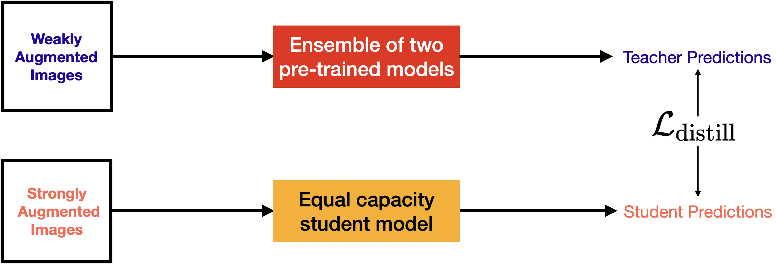
In an effort to unify our iterative training procedure, we also experimented with techniques like the Noisy Student Training [38] method to, but this method did not fare well. Following the recipes of [38], we performed self-training with noise injected only to the training data. We used the ensemble of the U-Net and U-Net++ models as a teacher and a U-Net model (with MobileNetV2 backend) as a student. During training the student model our data consists of both the training and test data. This training pipeline is depicted in Figure 3. With this pipeline we obtained an IoU of 0.75, which is inferior to the approach we ultimately followed. We also note that this method requires significantly less compute compared to the approach we ultimately settled with. So, if IoU can be traded with limited compute requirements, this method still yields competitive results. In regard to Figure 3, $\mathcal{L}_{\text{distill}}$ is defined as per (3).

$$\left.\mathcal{L}_{\text{distill }}=(1-\alpha)\mathcal{L}_{\text{DICE}}\left(\text{s\_preds}\left(Z_{s}\right),y\right)+\alpha\mathcal{L}_{\mathrm{KL}}(\text{(s\_preds}/\tau),(\text{t\_preds}/\tau)\right),$$ (3)

where $s\_preds$ and $t\_preds$ denote predictions from the student and teacher networks respectively, $y$ is a vector of containing the ground-truth segmentation maps, $\alpha$ is a scalar that controls the contributions from $\mathcal{L}_{\text{DICE}}$ and $\mathcal{L}_{\mathrm{KL}}$ (KL-Divergence), and $\tau$ is a scalar denoting the temperature [14]. Note that for computing $\mathcal{L}_{\text{DICE}}$ in 3, we use the predictions obtained from strongly augmented original training set and their ground-truth segmentation maps.

From our experiments, we believe that with additional tweaks inspired from [47, 4] it is possible to further push this performance and we aim to explore this as future work.

Figure 3: Our semi-supervised training pipeline based on Noisy Student Training [38].

Appendix C Supplemental Figures

Figure 4: Raw data (VV and VH tiles) provided by the competition, and the state of water body before and after flood. The composite RGB or colour image which we use for training, is generated using the ESA Polarimetry guidelines with VV channel for red, VH channel for green and the ratio $|VV|/|VH|$ for blue. All images are a random sample from the training set. We note the visible grains in different directions potentially due to recently harvested agricultural fields from Bangladesh. North Alabama show various artifacts including potential swath gaps due to differences in satellite coverage, while the RGB color range in Nebraska is unique. The North Alabama image with swath gaps is kept because of at least some positive ground truth artifacts (after flood) available.

Figure 5: Noisy images either due to swath gaps or completely empty ones which occur when the VV and VH images do not align and are filtered out. Note that ground truth artifacts are unfavorable as they do not provide a positive example.

References

- [1] Aimoldin Anuar. Siim-acr pneumothorax segmentation winning solution. https://www.kaggle.com/c/siim-acr-pneumothorax-segmentation/discussion/107824, 2019.
- [2] Anurag Arnab, Shuai Zheng, Sadeep Jayasumana, Bernardino Romera-Paredes, Måns Larsson, Alexander Kirillov, Bogdan Savchynskyy, Carsten Rother, Fredrik Kahl, and Philip H.S. Torr. Conditional random fields meet deep neural networks for semantic segmentation: Combining probabilistic graphical models with deep learning for structured prediction. IEEE Signal Processing Magazine, 35(1):37–52, 2018.
- [3] Yauhen Babakhin. How to cook pseudo-labels. https://www.youtube.com/watch?v=SsnWM1xWDu4, 2019.
- [4] David Berthelot, Rebecca Roelofs, Kihyuk Sohn, Nicholas Carlini, and Alex Kurakin. Adamatch: A unified approach to semi-supervised learning and domain adaptation, 2021.
- [5] Lucas Beyer. pydensecrf. https://github.com/lucasb-eyer/pydensecrf, 2015.
- [6] Alexander Buslaev, Vladimir I. Iglovikov, Eugene Khvedchenya, Alex Parinov, Mikhail Druzhinin, and Alexandr A. Kalinin. Albumentations: Fast and flexible image augmentations. Information, 11(2), 2020.
- [7] O. Chapelle, B. Scholkopf, and A. Zien, Eds. Semi-supervised learning (chapelle, o. et al., eds.; 2006) [book reviews]. IEEE Transactions on Neural Networks, 20(3):542–542, 2009.
- [8] Abhishek Chaurasia and Eugenio Culurciello. Linknet: Exploiting encoder representations for efficient semantic segmentation. 2017 IEEE Visual Communications and Image Processing (VCIP), Dec 2017.
- [9] Liang-Chieh Chen, George Papandreou, Iasonas Kokkinos, Kevin Murphy, and Alan L. Yuille. Deeplab: Semantic image segmentation with deep convolutional nets, atrous convolution, and fully connected crfs. IEEE Transactions on Pattern Analysis and Machine Intelligence, 40(4):834–848, 2018.
- [10] Liang-Chieh Chen, Yukun Zhu, George Papandreou, Florian Schroff, and Hartwig Adam. Encoder-decoder with atrous separable convolution for semantic image segmentation. In Vittorio Ferrari, Martial Hebert, Cristian Sminchisescu, and Yair Weiss, editors, Computer Vision – ECCV 2018, pages 833–851, Cham, 2018. Springer International Publishing.
- [11] Sarah Chen, Esther Cao, Anirudh Koul, Siddha Ganju, Satyarth Praveen, and Meher Anand Kasam. Reducing effects of swath gaps in unsupervised machine learning. Committee on Space Research Machine Learning for Space Sciences Workshop, Cross-Disciplinary Workshop on Cloud Computing, 2021.
- [12] Ron Hagensieker, Ribana Roscher, Johannes Rosentreter, Benjamin Jakimow, and Björn Waske. Tropical land use land cover mapping in pará (brazil) using discriminative markov random fields and multi-temporal terrasar-x data. International Journal of Applied Earth Observation and Geoinformation, 63:244–256, 2017.
- [13] Kaiming He, Xiangyu Zhang, Shaoqing Ren, and Jian Sun. Deep residual learning for image recognition. In 2016 IEEE Conference on Computer Vision and Pattern Recognition (CVPR), pages 770–778, 2016.
- [14] Geoffrey Hinton, Oriol Vinyals, and Jeffrey Dean. Distilling the knowledge in a neural network. In NIPS Deep Learning and Representation Learning Workshop, 2015.
- [15] Gao Huang, Yu Sun, Zhuang Liu, Daniel Sedra, and Kilian Q. Weinberger. Deep networks with stochastic depth. In Bastian Leibe, Jiri Matas, Nicu Sebe, and Max Welling, editors, Computer Vision – ECCV 2016, pages 646–661, Cham, 2016. Springer International Publishing.
- [16] Diederik P. Kingma and Jimmy Ba. Adam: A method for stochastic optimization. In Yoshua Bengio and Yann LeCun, editors, 3rd International Conference on Learning Representations, ICLR 2015, San Diego, CA, USA, May 7-9, 2015, Conference Track Proceedings, 2015.
- [17] Philipp Krähenbühl and Vladlen Koltun. Efficient inference in fully connected crfs with gaussian edge potentials. Advances in Neural Information Processing Systems 24 (2011) 109-117, abs/1210.5644, 2012.
- [18] Balaji Lakshminarayanan, Alexander Pritzel, and Charles Blundell. Simple and scalable predictive uncertainty estimation using deep ensembles. In I. Guyon, U. V. Luxburg, S. Bengio, H. Wallach, R. Fergus, S. Vishwanathan, and R. Garnett, editors, Advances in Neural Information Processing Systems, volume 30. Curran Associates, Inc., 2017.
- [19] Dong-Hyun Lee. Pseudo-label : The simple and efficient semi-supervised learning method for deep neural networks. ICML 2013 Workshop : Challenges in Representation Learning (WREPL), 07 2013.
- [20] Tsung-Yi Lin, Piotr Dollár, Ross B. Girshick, Kaiming He, Bharath Hariharan, and Serge J. Belongie. Feature pyramid networks for object detection. CoRR, abs/1612.03144, 2016.
- [21] Tsung-Yi Lin, Priya Goyal, Ross B. Girshick, Kaiming He, and Piotr Dollár. Focal loss for dense object detection. CoRR, abs/1708.02002, 2017.
- [22] Ilya Loshchilov and Frank Hutter. SGDR: stochastic gradient descent with warm restarts. In 5th International Conference on Learning Representations, ICLR 2017, Toulon, France, April 24-26, 2017, Conference Track Proceedings. OpenReview.net, 2017.
- [23] Gonzalo Mateo-Garcia, Joshua Veitch-Michaelis, Lewis Smith, Silviu Vlad Oprea, Guy Schumann, Yarin Gal, Atılım Güneş Baydin, and Dietmar Backes. Towards global flood mapping onboard low cost satellites with machine learning. Nature Publishing Group, Mar 2021.
- [24] Paulius Micikevicius, Sharan Narang, Jonah Alben, Gregory Diamos, Erich Elsen, David Garcia, Boris Ginsburg, Michael Houston, Oleksii Kuchaiev, Ganesh Venkatesh, and Hao Wu. Mixed precision training. In International Conference on Learning Representations, 2018.
- [25] Fausto Milletari, Nassir Navab, and Seyed-Ahmad Ahmadi. V-net: Fully convolutional neural networks for volumetric medical image segmentation. CoRR, abs/1606.04797, 2016.
- [26] Philipp Moritz, Robert Nishihara, Stephanie Wang, Alexey Tumanov, Richard Liaw, Eric Liang, Melih Elibol, Zongheng Yang, William Paul, Michael I. Jordan, and Ion Stoica. Ray: A distributed framework for emerging ai applications. In Proceedings of the 13th USENIX Conference on Operating Systems Design and Implementation, OSDI’18, page 561–577, USA, 2018. USENIX Association.
- [27] Amir Mosavi, Pinar Ozturk, and Kwok-wing Chau. Flood prediction using machine learning models: Literature review. Water, 10(11), 2018.
- [28] Adam Paszke, Sam Gross, Francisco Massa, Adam Lerer, James Bradbury, Gregory Chanan, Trevor Killeen, Zeming Lin, Natalia Gimelshein, Luca Antiga, Alban Desmaison, Andreas Kopf, Edward Yang, Zachary DeVito, Martin Raison, Alykhan Tejani, Sasank Chilamkurthy, Benoit Steiner, Lu Fang, Junjie Bai, and Soumith Chintala. Pytorch: An imperative style, high-performance deep learning library. In H. Wallach, H. Larochelle, A. Beygelzimer, F. d'Alché-Buc, E. Fox, and R. Garnett, editors, Advances in Neural Information Processing Systems 32, pages 8024–8035. Curran Associates, Inc., 2019.
- [29] Ilija Radosavovic, Raj Prateek Kosaraju, Ross Girshick, Kaiming He, and Piotr Dollár. Designing network design spaces. In 2020 IEEE/CVF Conference on Computer Vision and Pattern Recognition (CVPR), pages 10425–10433, 2020.
- [30] Olaf Ronneberger, Philipp Fischer, and Thomas Brox. U-net: Convolutional networks for biomedical image segmentation. In Nassir Navab, Joachim Hornegger, William M. Wells, and Alejandro F. Frangi, editors, Medical Image Computing and Computer-Assisted Intervention – MICCAI 2015, pages 234–241, Cham, 2015. Springer International Publishing.
- [31] Mark Sandler, Andrew G. Howard, Menglong Zhu, Andrey Zhmoginov, and Liang-Chieh Chen. Inverted residuals and linear bottlenecks: Mobile networks for classification, detection and segmentation. IEEE Conference on Computer Vision and Pattern Recognition (CVPR), 2018, pp. 4510-4520, abs/1801.04381, 2018.
- [32] Puneet Sharma. Dihedral group d4—a new feature extraction algorithm. Symmetry, 12(4), 2020.
- [33] Kihyuk Sohn, David Berthelot, Nicholas Carlini, Zizhao Zhang, Han Zhang, Colin A Raffel, Ekin Dogus Cubuk, Alexey Kurakin, and Chun-Liang Li. Fixmatch: Simplifying semi-supervised learning with consistency and confidence. In H. Larochelle, M. Ranzato, R. Hadsell, M. F. Balcan, and H. Lin, editors, Advances in Neural Information Processing Systems, volume 33, pages 596–608. Curran Associates, Inc., 2020.
- [34] Nitish Srivastava, Geoffrey Hinton, Alex Krizhevsky, Ilya Sutskever, and Ruslan Salakhutdinov. Dropout: A simple way to prevent neural networks from overfitting. J. Mach. Learn. Res., 15(1):1929–1958, Jan. 2014.
- [35] B. Tellman, J. A. Sullivan, C. Kuhn, A. J. Kettner, C. S. Doyle, G. R. Brakenridge, T. A. Erickson, and D. A. Slayback. Satellite imaging reveals increased proportion of population exposed to floods. Nature Publishing Group, Aug 2021.
- [36] Marc Wieland and Sandro Martinis. A modular processing chain for automated flood monitoring from multi-spectral satellite data. Remote Sensing, 11(19), 2019.
- [37] Ross Wightman. Pytorch image models. https://github.com/rwightman/pytorch-image-models, 2019.
- [38] Qizhe Xie, Minh-Thang Luong, Eduard Hovy, and Quoc V. Le. Self-training with noisy student improves imagenet classification. In 2020 IEEE/CVF Conference on Computer Vision and Pattern Recognition (CVPR), pages 10684–10695, 2020.
- [39] Pavel Yakubovskiy. Image test time augmentation with pytorch. https://github.com/qubvel/ttach, 2020.
- [40] Pavel Yakubovskiy. Segmentation models pytorch. https://github.com/qubvel/segmentation_models.pytorch, 2020.
- [41] Yaxin Zhao, Jichao Jiao, and Tangkun Zhang. Manet: Multimodal attention network based point- view fusion for 3d shape recognition, 2020.
- [42] Shuai Zheng, Sadeep Jayasumana, Bernardino Romera-Paredes, Vibhav Vineet, Zhizhong Su, Dalong Du, Chang Huang, and Philip H. S. Torr. Conditional random fields as recurrent neural networks. CoRR, abs/1502.03240, 2015.
- [43] Zongwei Zhou, Md Mahfuzur Rahman Siddiquee, Nima Tajbakhsh, and Jianming Liang. Unet++: A nested u-net architecture for medical image segmentation. 4th Deep Learning in Medical Image Analysis (DLMIA) Workshop, abs/1807.10165, 2018.
- [44] Xiaojin Zhu. Semi-supervised learning literature survey. Technical Report 1530, Computer Sciences, University of Wisconsin-Madison, 2005.
- [45] Xiaojin Zhu and Andrew B. Goldberg. Introduction to semi-supervised learning. Synthesis Lectures on Artificial Intelligence and Machine Learning, 3(1):1–130, 2009.
- [46] Barret Zoph, Golnaz Ghiasi, Tsung-Yi Lin, Yin Cui, Hanxiao Liu, Ekin Dogus Cubuk, and Quoc Le. Rethinking pre-training and self-training. In H. Larochelle, M. Ranzato, R. Hadsell, M. F. Balcan, and H. Lin, editors, Advances in Neural Information Processing Systems, volume 33, pages 3833–3845. Curran Associates, Inc., 2020.
- [47] Yuliang Zou, Zizhao Zhang, Han Zhang, Chun-Liang Li, Xiao Bian, Jia-Bin Huang, and Tomas Pfister. Pseudoseg: Designing pseudo labels for semantic segmentation. In International Conference on Learning Representations, 2021.