.pdfpng.pngconvert #1

Best Subset Selection: Statistical Computing Meets Quantum Computing

Abstract

With the rapid development of quantum computers, quantum algorithms have been studied extensively. However, quantum algorithms tackling statistical problems are still lacking. In this paper, we propose a novel non-oracular quantum adaptive search (QAS) method for the best subset selection problems. QAS performs almost identically to the naive best subset selection method but reduces its computational complexity from $O(D)$ to $O(\sqrt{D}\log_{2}D)$, where $D=2^{p}$ is the total number of subsets over $p$ covariates. Unlike existing quantum search algorithms, QAS does not require the oracle information of the true solution state and hence is applicable to various statistical learning problems with random observations. Theoretically, we prove QAS attains any arbitrary success probability $q\in(0.5,1)$ within $O(\log_{2}D)$ iterations. When the underlying regression model is linear, we propose a quantum linear prediction method that is faster than its classical counterpart. We further introduce a hybrid quantum-classical strategy to avoid the capacity bottleneck of existing quantum computing systems and boost the success probability of QAS by majority voting. The effectiveness of this strategy is justified by both theoretical analysis and extensive empirical experiments on quantum and classical computers.

Keywords: hybrid quantum-classical strategy, majority voting, non-oracular quantum search, quantum experiments, quantum linear prediction.

1 Introduction

The rapid advance in science and technology in the past decade makes the quantum computer a reality, offering researchers an unprecedented opportunity to tackle more complex research challenges. Unlike classical computers depend on a classical bit having a state of either 0 or 1, a quantum computer operates on quantum processing units, quantum bits (or qubits), which can be in a state 0, 1, or both simultaneously due to the superposition property. The $n$ qubits create $2^{n}$ different states for the system that are superposed on each other. The superposition enables researchers to perform computations using all of those $2^{n}$ states simultaneously. In contrast, in classical computing, one conducts computations with one state at-a-time among these $2^{n}$ states. Consequently, one has to repeat the computations $2^{n}$ times in classical computing to get the quantum computation results. (Nielsen and Chuang,, 2010). Such a paradigm change has motivated significant developments of quantum algorithms in many areas, e.g., algebraic number theory (Shor,, 1999; Hallgren,, 2002; Van Dam and Shparlinski,, 2008), scientific simulations (Abrams and Lloyd,, 1997; Byrnes and Yamamoto,, 2006; Kassal et al.,, 2008; Wang,, 2011; Hu and Wang,, 2020), optimization (Jordan,, 2005; Jansen et al.,, 2007; Harrow et al.,, 2009), and many more.

The opportunity, however, has not yet been fully utilized by statisticians, because there are significant challenges to developing quantum search algorithms to solve statistical problems. First, a quantum computer does not provide deterministic results but instead gives a different result each time we run an algorithm according to some probability distribution. For example, if we search the smallest number in a set of numbers using a classical computer, the result is determined if the algorithm is deterministic. However, a quantum computer output the smallest number with a certain probability. That is, a quantum computer may output another number other than the correct result. Second, existing quantum search algorithms, in general, depend on an oracle function to decide if an outcome is a solution or not. For example, the celebrated Grover’s algorithm (Grover,, 1997) requires an oracle function that can map all solutions to state 1 and all non-solutions to state 0. However, such an oracle function is usually not available in practice. When the oracle is inaccurate, Grover’s algorithm can perform as bad as a random guess which will be demonstrated in our numerical experiments. Third, the current public available general-purpose quantum computer, such as the quantum computing system developed by IBM, only has a few dozens of qubits, and thus allows very small piloting projects.

In this paper, we investigate the possibility of solving the best subset selection problem on a quantum computing system. The best subset selection problem can be described as follows: Given a response $y$ and multiple predictors $x_{1},x_{2},\ldots,x_{p}$, we aim to find the best subset among $x_{1},x_{2},\ldots,x_{p}$ to fit the response $y$. There are $2^{p}$ candidate subsets. For $p=30$, we have more than one billion candidate subsets. Currently, there is no quantum algorithm specifically designed for the best subset selection problem. We propose a novel non-oracular quantum method named quantum adaptive search (QAS). To overcome the aforementioned limitations, we randomly choose a model as our initial guess of the best subset. QAS starts with an equally weighted superposition of the rest candidate models and iteratively updates the superposition towards the direction that minimizes the $\ell_{2}$ loss. Within each iteration, the new superposition is compared with the old one through a local evaluation function which does not require any oracle information of the true solution. After the number of iterations, the result will replace our initial guess. We then repeat the above procedures until no more replacement can be made. Since the output of the quantum computer is random, we further introduce a hybrid quantum-classical strategy and boost the success probability of outputting the best subset by a majority voting.

Our theoretical and methodological contributions are as follows. First, we design an iterative algorithm to eliminate the requirement of an oracle function in the quantum algorithm. Second, we design a majority voting so that we have a high probability to get the correct solution from the algorithm. Moreover, for the best subset selection problem over $D=2^{p}$ candidate models, within $O(\log_{2}D)$ iterations, QAS converges to a superposition that heavily weighs on the solution state and hence outputs the exact solution with a high probability. In contrast, a classic computing algorithm requires $O(D)$ quires to search for the best model. Last but not least, the computational complexity of QAS is upper bounded by the order $O(\sqrt{D}\log_{2}D)$ which is only a $\log_{2}D$ factor larger than the theoretical lower bound for any oracular quantum search algorithms (Bennett et al.,, 1997).

Our empirical contribution is that we explore the simulation and real data analysis in IBM Quantum Experience, which is a publicly available cloud-based quantum computing system. The code and tutorial are publicly available. The exploration will facilitate the subsequent development in quantum algorithm development for solving statistical problems.

The rest of the paper is organized as follows. We review the state-of-the-art quantum search algorithm and its limitation in Section 2. In Section 3, we propose a novel quantum adaptive search (QAS) algorithm and discuss its intuition and theoretical properties. We then introduce a quantum linear prediction algorithm for computing the criterion. In Section 4 , we introduce a quantum-classical hybrid strategy to improve the stability of quantum best subset selection. In Sections 5 and 6, we evaluate the empirical performance of the proposed method via extensive experiments on quantum and classical computers. Section 7 concludes the paper with a few remarks. Due to the limitation of space, the proofs of main theoretical results, additional simulation results, and a real data application are relegated to a supplemental material.

2 Review of quantum search algorithm

2.1 Notations and definitions

To facilitate the discussion in the paper, we review some essential notations and definitions used in quantum computing that may be alien to the audience of statistics. We refer to Nielsen and Chuang, (2010) and Schuld and Petruccione, (2018) for more detailed tutorials of quantum computing. We start by introducing the linear algebra notations used in quantum mechanics, which were invented by Paul Dirac. In Dirac’s notation, a column vector ${\bf a}$ is denoted by $\ket{a}$ which reads as ${\bf a}$ in a ‘ket’. Typical vector space of interest in quantum computing is a Hilbert space $\mathcal{H}$ of dimension $D=2^{p}$ with a positive integer $p$. For a vector $\ket{a}\in\mathcal{H}$, we denote its dual vector as $\bra{a}$ (reads as $\bf a$ in a ‘bra’), which is an element of $\mathcal{H}^{*}$. Besides, $\mathcal{H}$ and $\mathcal{H}^{*}$ together naturally induce an inner product $\braket{a}{b}=\braket{{\bf a},{\bf b}}$, which is also known as a ‘bra-ket’. We say $\ket{a}$ is a unit vector if $\braket{a}{a}=1$.

The framework of quantum computing resides in a state-space postulate which describes the state of a system by a unit vector in a Hilbert space. A state of a qubit can be described by a unit vector $\ket{\psi}$ in a two-dimensional Hilbert space. A superposition, as the linear combination of the states in one qubit, can be defined as

$$\ket{\psi}=\phi_{0}\ket{0}+\phi_{1}\ket{1},$$

where coefficients $\phi_{0}$ and $\phi_{1}$ satisfy $|\phi_{0}|^{2}+|\phi_{1}|^{2}=1$. Now suppose that we have two qubits and the system has four orthonormal states $\ket{00},\ket{01},\ket{10},\ket{11}$. Then, a superposition can be represented as

$$\ket{\psi}=\phi_{0}\ket{00}+\phi_{1}\ket{01}+\phi_{2}\ket{10}+\phi_{3}\ket{11},$$

where coefficients $\phi_{0}$, $\phi_{1}$, $\phi_{2}$, $\phi_{3}$ satisfiy $|\phi_{0}|^{2}+|\phi_{1}|^{2}+|\phi_{2}|^{2}+|\phi_{3}|^{2}=1$. Analogously, a quantum computer of $p$ qubits can represent a state of a system by a unit vector $\ket{\psi}$ in a $D=2^{p}$ dimensional Hilbert space $\mathcal{H}$. Let ${\mathcal{B}}=\{\ket{b_{i}}\}_{i=0}^{D-1}$ be an orthonormal basis of $\mathcal{H}$. Every superposition $\ket{\psi}\in\mathcal{H}$ can be represented as

$$\ket{\psi}=\sum\limits_{i=0}^{D-1}\phi_{i}\ket{b_{i}},$$ (1)

where $\phi_{0},\ \ldots,\ \phi_{D-1}$ is a set of coefficients with $\phi_{i}=\braket{b_{i}}{\psi}$ and $\sum_{i=0}^{D-1}|\phi_{i}|^{2}=1$.

Another salient feature of quantum computing is the measurement of a quantum system yields a probabilistic outcome rather than a deterministic one. Suppose the superposition $\ket{\psi}$ in (1) is measured, it collapses to a random state in ${\mathcal{B}}$. In addition, the probability we observe $\ket{b_{i}}$ is $|\phi_{i}|^{2}$ for $i=0,\ldots,D-1$.

Different from a classical computer with logic gates, e.g., AND and NOT gates, a quantum computer is built with quantum gates. These quantum gates not only have the logic gates mentioned above but also include the new gates that are not available in classical computers. For example, the Hadamard gate enables the rotations and reflections of the input states. Some quantum algorithms that make use of these new gates have shown some remarkable results that significantly outperform the algorithms in classical computers.

2.2 Grover’s algorithm

The best subset selection problem can be decomposed into two subproblems: (1) What is the criterion for the best? (2) Given the criterion, which subset is the best? For the first subproblem, there are many criteria, e.g, AIC, BIC, cross-validation, and mean squared error. For the second subproblem, searching for the best is challenging if the number of candidate subsets is super-large. We shall review Grover’s algorithm, which is the most popular quantum searching algorithm for the second subproblem.

Recall that given $p$ predictors, there are $D=2^{p}$ candidate subsets, from which we aim to find the best subset. Once the best criterion is chosen and applied to each subset, we have $D=2^{p}$ criterion values computed for all subsets. We aim to find the solution (e.g. the smallest or the largest value) from $D=2^{p}$ elements, which are indexed by $0,1,\ldots,D-1$. To ease the presentation, we assume there are no tied solutions although the discussions in this paper can be easily generalized to such cases. In the language of quantum computing, each index is regarded as a state, which can be modeled by a unit vector in an orthonormal basis ${\cal D}=\{\ket{i}\})_{i=0}^{D-1}$ of a $D$ dimensional Hilbert space $\mathcal{H}$.

2.2.1 Geometric view of Grover’s algorithm

We now provide an intuitive geometric presentation of Grover’s algorithm which is summarized in Algorithm 1 below. Denote the solution state by $\ket{k}$ and the average of all non-solution states by $\ket{\zeta}=\frac{1}{\sqrt{D-1}}\sum\limits_{i\neq k}\ket{i}$. Notice that $\ket{\zeta}$ is orthogonal to the solution state $\ket{k}$. We plot them as $x$-axis and $y$-axis in Figure 1. Grover’s algorithm is initialized with a superposition as the equally weighted average of all states $\ket{i}$, $i=0,\ldots,D-1$. To be specific, the initial superposition is defined as

$$\ket{\psi_{0}}=\frac{1}{\sqrt{D}}\sum\limits_{i=0}^{D-1}\ket{i}.$$

Denote the angel between the initial superposition $\ket{\psi_{0}}$ and $\ket{\zeta}$ by $\theta$. It is easy to see that $\sin\theta=\frac{1}{\sqrt{D}}$.

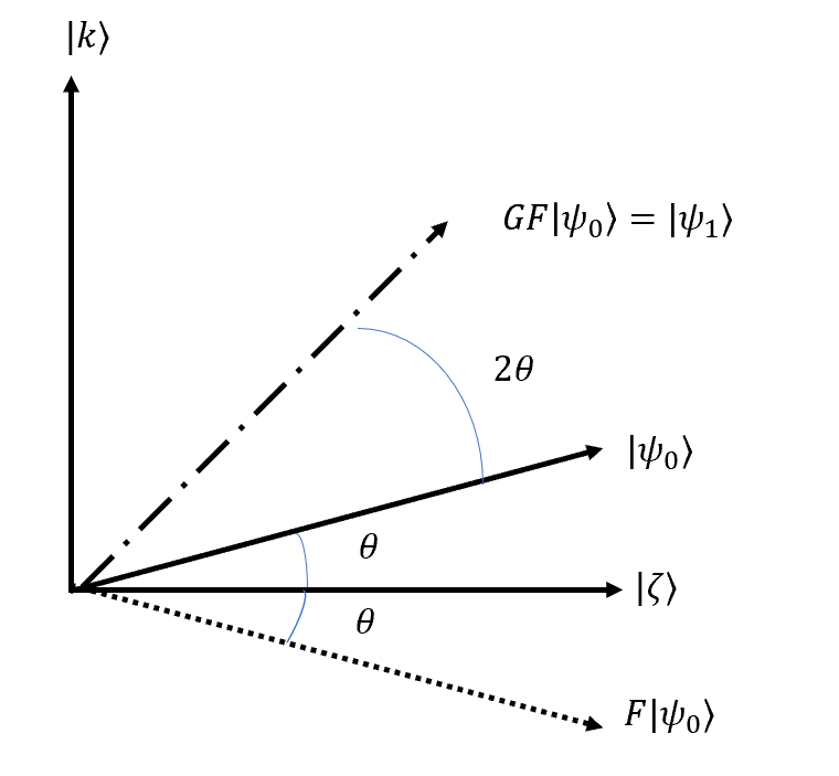
Figure 1: Geometrical visualization of the two steps in the first Grover’s operation.

The first iteration of Grover’s algorithm contains two operations. The first operation reflects $\ket{\psi_{0}}$ with respect to $\ket{\zeta}$ to get $F\ket{\psi_{0}}$, The second operation reflects $F\ket{\psi_{0}}$ with respect to $\ket{\psi_{0}}$ to get $GF\ket{\psi_{0}}$, which is our new superposition, denoted by $\ket{\psi_{1}}$. As a result, the angle between $\ket{\psi_{1}}$ and $\ket{\zeta}$ is $3\theta$. Figure 1 provides a visualization of the two operations in the first Grover’s operation. Then, Grover’s algorithm iteratively repeats the above two operations, i.e, a reflection w.r.t. $\ket{\zeta}$ and then a reflection w.r.t. $\ket{\psi_{0}}$. After the $j$th iteration, the the angle between $\ket{\psi_{j}}$ and $\ket{\zeta}$ is $(2j+1)\theta$. The iteration terminates if the $j$th state $\ket{\psi_{j}}$ coincides with the solution state $\ket{k}$, i.e., $\ket{\psi_{j}}=\ket{k}$, which implies that

$$(2j+1)\theta=\pi/2.$$ (2)

The typical motivation to use quantum search algorithm is that the number of candidate set $D$ is large. When $D$ is large, i.e., $\theta$ is small, we can approximate the angle by

$$\theta\approx\sin\theta=\frac{1}{\sqrt{D}}.$$ (3)

Substituting (3) into (2), we have $(2j+1)/\sqrt{D}=\pi/2$, which yields $j$ is approximately $\sqrt{D}\pi/4$. This is a remarkable result since the number of iteration is in the order of $O(\sqrt{D})$. Grover’s algorithm can be easily extended to a search problem with $M>1$ solutions, where the number of iteration $j$ is approximately $\sqrt{D/M}\pi/4$. See Boyer et al., (1998) for more detailed discussions.

2.2.2 Technical details of Grover’s algorithm

Now we present Grover’s algorithm with more mathematical rigor. Grover’s algorithm assumes that we are provided with an quantum oracle evaluation function $S(\cdot)$, which can recognize the solution to the search problem. That is, suppose that index $k\in\{0,\ldots,D-1\}$ corresponds to the best subset, we have $S(\ket{k})=1$ and $S(\ket{i})=0$ for $i\neq k$. Recall that, Grover’s algorithm is initialized with the following superposition

$$\ket{\psi_{0}}=\frac{1}{\sqrt{D}}\sum\limits_{i=0}^{D-1}\ket{i}\equiv c_{0}\ket{k}+d_{0}\sum\limits_{i\neq k}\ket{i},$$

where $c_{0}=d_{0}=\frac{1}{\sqrt{D}}$. Then, Grover’s algorithm updates $c$ and $d$ in an iterative manner. In the $j$th iteration, Grover’s algorithm applies the following two operations to the current superposition $\ket{\psi_{j-1}}=c_{j-1}\ket{k}+d_{j-1}\sum\limits_{i\neq k}\ket{i}$,

• A flip operation $F$ to $\ket{\psi_{j-1}}$, where $F\ket{i}=\left(1-2S(\ket{i})\right)\ket{i}$. In other words, $F\ket{k}=-\ket{k}$ and $F\ket{i}=\ket{i}$ for $i\neq k$.

• A Grover’s diffusion operation $G$ to $F\ket{\psi_{j-1}}$, where $G=2\ket{\psi_{0}}\bra{\psi_{0}}-{\bm{I}}_{D}$ and ${\bm{I}}_{D}$ is a $D\times D$ identity matrix.

In the rest of this paper, we call the two operations together, i.e. $GF$, as Grover’s operation

After the $j$th iteration, the superposition $\ket{\psi_{j-1}}$ is updated to

$$\ket{\psi_{j}}=GF\ket{\psi_{j-1}}=c_{j}\ket{k}+d_{j}\sum\limits_{i\neq k}\ket{i},$$

where the coefficients $c_{j}$ and $d_{j}$ satisfy

$$\begin{cases}c_{j}=\frac{D-2}{D}c_{j-1}+\frac{2(D-1)}{D}d_{j-1},\\ d_{j}=\frac{D-2}{D}d_{j-1}-\frac{2}{D}c_{j-1}.\end{cases}$$

Let $\theta$ be the angle that satisfies $\sin^{2}\theta=\frac{1}{D}$. The coefficients $c_{j}$ and $d_{j}$ admit a closed form (Nielsen and Chuang,, 2010),

$$\begin{cases}c_{j}=\sin\big{(}(2j+1)\theta\big{)},\\ d_{j}=\frac{1}{\sqrt{D-1}}\cos\big{(}(2j+1)\theta\big{)}.\end{cases}$$

Algorithm 1 Grover’s algorithm

Input: An orthonormal basis $\mathcal{D}$ of size $D=2^{p}$, a binary evaluation function $S$ associated with an oracle state $|k\rangle$, such that $S(\ket{k})=1$ and $S(\ket{i})=0$ for $i\neq k$. Number of iterations $\tau=\lceil\pi\sqrt{D}/4\rceil$, where $\lceil\cdot\rceil$ is the ceiling function.

Initialization Prepare an equally weighted superposition on a quantum register of $p$-qubits $\ket{\psi_{0}}=\frac{1}{\sqrt{D}}\sum_{i=0}^{D-1}|i\rangle$.

for $j=1,\ldots,\tau$ do

     Grover’s operation: Let $\ket{\psi_{j}}=GF\ket{\psi_{j-1}}$, where $F\ket{i}=\left(1-2S(\ket{i}\right)\ket{i}$,

     $G=2\ket{\psi_{0}}\bra{\psi_{0}}-{\bm{I}}_{D}$, and ${\bm{I}}_{D}$ is a $D\times D$ identity matrix.

end for

Output: Measure the latest superposition $\ket{\psi_{\tau}}$ on the quantum register.

2.2.3 Significance and challenges of Grover’s algorithm

Grover, (1997) proposed a quantum search algorithm with a success probability of at least 50%. The computational complexity of Grover’s algorithm is of the order $O(\sqrt{D})$. Bennett et al., (1997) showed that this rate is optimal, up to a constant, among all possible quantum search algorithms. In contrast, any classical search algorithm needs to query the system for at least $0.5D$ times to solve the searching problem with a 50% or higher success probability. As a result, most classical search algorithms have the computational complexity of the order $O(D)$.

Grover’s algorithm is a quantum algorithm that depends on an oracle evaluation function that maps the solution state to 1 and all other states to 0. However, such a piece of oracle information is usually not available in statistical problems including the best subset selection. When we have no oracle information of the solution state at all, the oracle evaluation function can only be constructed by a randomly selected solution state. Then, Grover’s algorithm is highly likely to rotate the initial superposition in a wrong direction and the output of the algorithm can be as bad as a random guess. We empirically demonstrate this phenomenon in Section 5.2.

3 Best subset selection with quantum adaptive search

In this section, we first review the best subset selection problem. We then propose a novel quantum search algorithm named quantum adaptive search (QAS) which aims to overcome the aforementioned limitation of Grover’s algorithm. We also provide a quantum linear prediction (QLP) method to compute the loss function.

3.1 Review of best subset selection

Best subset selection has been a classical and fundamental method for linear regressions (e.g. Hocking and Leslie,, 1967; Beale et al.,, 1967; Shen et al.,, 2012; Fan et al.,, 2020). When the covariates contain redundant information for the response, selecting a parsimonious best subset of covariates may improve the model interpretability as well as the prediction performance. The best subset selection for linear regression can be formulated as

$$\min_{\bm{\beta}\in\mathbb{R}^{p}}\|\bm{Y}-\bm{X}\bm{\beta}\|_{2}^{2}\quad\text{subject to}\quad\|\bm{\beta}\|_{0}\leq t,$$ (4)

where $\bm{Y}=(y_{1},\ \ldots,\ y_{n})^{\mathrm{\scriptstyle T}}\in\mathbb{R}^{n}$ is a response vector, $\bm{X}=(x_{i,j})_{1\leq i\leq n,1\leq j\leq p}\in\mathbb{R}^{n\times p}$ is a design matrix of covariates and $\bm{\beta}=(\beta_{1},\ \ldots,\ \beta_{p})^{\mathrm{\scriptstyle T}}\in\mathbb{R}^{p}$ is a vector of unknown regression coefficients. Throughout this paper, we assume $\bm{Y}$ and $\bm{X}$ are centered for the simplicity of presentation. Further, $\|\bm{\beta}\|_{0}$ is the $\ell_{0}$ norm of $\bm{\beta}$ and $0\leq t\leq\min{(n,p)}$ is a subset size. In general, solving (4) is a non-convex optimization problem. Without a convex relaxation or a stage-wise approximation, the optimization involves a combinatorial search over all subsets of sizes $\{1,\ \ldots,\ \min(n,p)\}$ and hence is an NP-hard problem (Welch,, 1982; Natarajan,, 1995). Therefore, seeking the exact solution of (4) is usually computationally intractable when $p$ is moderate or large.

To overcome the computational bottleneck of the best subset selection, many alternative and approximate approaches have been developed and carefully studied. Stepwise regression methods (e.g. Efroymson,, 1960; Draper and Smith,, 1966) sequentially add or eliminate covariates according to their marginal contributions to the response condition on the existing model. Stepwise regression methods speed up the best subset selection as they only optimize (4) over a subset of all candidates, and hence their solutions may not coincide with the solution of (4). However, stepwise regression methods suffer from the instability issue in high dimensional regime (Breiman,, 1996). Regularized regression methods suggest to relax the nonconvex $\ell_{0}$ norm in (4) by various convex or nonconcave alternatives. A celebrated member in the house is LASSO (Tibshirani,, 1996) which solves an $\ell_{1}$ regularized problem instead. Elegant statistical properties and promising numerical performance soon made regularized regression a popular research topic in statistics, machine learning and other data science related areas. We refer to basis pursuit (Chen and Donoho,, 1994), SCAD (Fan and Li,, 2001), elastic net (Zou and Hastie,, 2005), adaptive LASSO (Zou,, 2006), Dantzig selector (Candes and Tao,, 2007), nonnegative garrotte (Yuan and Lin,, 2007), and MCP (Zhang,, 2010), among many others. Though regularized regression methods can perform equivalent to or even better than the solution of (4) in certain scenarios (e.g. Zhao and Yu,, 2006; Fan et al.,, 2014; Hastie et al.,, 2020), they are not universal replacements for the best subset selection method. Nevertheless, solving (4) efficiently remains a statistically attractive and computationally challenging problem.

Recently, Bertsimas et al., (2016) has reviewed the best subset selection problem from a modern optimization point of view. Utilizing the algorithmic advances in mixed integer optimization, Bertsimas et al., (2016) proposed a highly optimized solver of (4) which is scalable to relatively large $n$ and $p$. Later, Hazimeh and Mazumder, (2018) considered a new hierarchy of necessary optimality conditions and propose to solve (4) by adding extra convex regularizations. Then, Hazimeh and Mazumder, (2018) developed an efficient algorithm based on coordinate descent and local combinatorial optimization. Such recent optimization developments push the frontier of computation for the best subset selection problems by a big margin.

3.2 Quantum adaptive search algorithm

Let us consider the best subset selection problem (4) and assume $n\geq p$ such that all $D=2^{p}$ subsets of $p$ covariates are attainable. When $n<p$, we only need to search over $\sum_{t=0}^{n}{p\choose t}<2^{p}$ subsets which is a less challenging combinatorial search problem.

3.2.1 Overview of quantum adaptive search algorithm

Recall that each subset of $\{1,\ \ldots,\ p\}$ can be encoded as a state in an orthonormal basis $\mathcal{D}=\{\ket{0},\ \ldots,\ \ket{D-1}\}$, which consists of $D=2^{p}$ elements of a Hilbert space $\mathcal{H}$. We define a state loss function $g(\cdot):\mathcal{H}\rightarrow\mathbb{R}$ by the mean squared error (MSE),

$$g(\ket{i})\equiv L_{n}(t;j_{1},\ \ldots,\ j_{t};\widehat{\beta}_{j_{1}},\ \ldots\ ,\widehat{\beta}_{j_{t}})=\frac{1}{n}\sum\limits_{i=1}^{n}\left(y_{i}-\sum_{l=1}^{t}\widehat{\beta}_{j_{l}}x_{i,j_{l}}\right)^{2},$$ (5)

where the state $\ket{i}\in\mathcal{D}$ is a vector in $\mathcal{H}$ that corresponds to the subset $\{j_{1},\ \ldots,\ j_{t}\}$, and $\widehat{\beta}_{j_{1}},\ \ldots\ ,\widehat{\beta}_{j_{t}}$ are the regression coefficient estimates obtained by minimizing (4) with fixed $t$ and $\{j_{1},\ \ldots,\ j_{t}\}$. Intuitively, the best subset corresponds to the state that minimizes the state loss function.

Now, we present the proposed non-oracular quantum adaptive search method, i.e. QAS, by three key steps as follows.

(1) Initialization: We choose an initial benchmark state $\ket{w}$ randomly from the set $\mathcal{D}=\{\ket{0},\ \ldots,\ \ket{D-1}\}$. Also, we pre-specify a learning rate $\lambda\in(0,1)$.

(2) Updating: We run Algorithm 1 on set $\mathcal{D}$ by inputting the benchmark state $\ket{w}$ and the number of iterations $\tau=\lceil\pi\lambda^{-m/2}/4\rceil$, where $m$ is a positive integer. Denote the output of Algorithm 1 as $\ket{w^{new}}$ which is a state in $\mathcal{D}$. Then, we compare $\ket{w^{new}}$ with $\ket{w}$ in terms of the state loss function $g(\cdot)$. If $g(\ket{w^{new}})<g(\ket{w})$, we update the current benchmark state $\ket{w}$ with $\ket{w^{new}}$, otherwise we do not update $\ket{w}$.

(3) Iteration and output: Start with $m=1$ and repeat the updating step. After each updating step, set $m=m+1$. The QAS stops when $m>C(\lambda)\ln{D}$, where $C(\lambda)$ is a positive constant that depends on the learning rate $\lambda$. Then, we measure the quantum register with the latest superposition. The output is the observed state in $\mathcal{D}$ and its corresponding subset.

Unlike Grover’s algorithm, QAS randomly selects a state in $\mathcal{D}$ as the benchmark state which does not require any oracle information of the solution state. Then, QAS iteratively updates the benchmark state towards the direction that reduces the state loss function. Besides, QAS is data-adaptive in the sense that it starts with a conservative learning step size (e.g. $m=1$) and gradually increases the learning step size as the benchmark state has been updated towards the truth. We summarize QAS in Algorithm 2 below.

Algorithm 2 Quantum adaptive search

Input: An orthonormal basis $\mathcal{D}$ of size $D=2^{p}$, a state loss function $g(\cdot)$ that maps a state in $\mathcal{D}$ to a real number, a learning rate $\lambda\in(0,1)$.

Initialization Set $m=1$. Randomly select a state in $\mathcal{D}$ as the initial benchmark state $\ket{w}$. Define a local evaluation function $S(\ \cdot\ ,\ket{w},g)$ such that $S(\ket{i},\ket{w},g)=1$ if $g(\ket{i})\leq g(\ket{w})$ and $S(\ket{i},\ket{w},g)=0$ if $g(\ket{i})>g(\ket{w})$.

repeat

     (1) Run Algorithm 1 by inputting $\mathcal{D}$, $S(\ \cdot\ ,\ket{w},g)$ and $\tau(m)=\lceil\pi\lambda^{-m/2}/4\rceil$.

     (2) Measure the quantum register and denote the readout by $\ket{w^{new}}$.

     (3) If $g(|w^{new}\rangle)<g(|w\rangle)$, set $|w\rangle=|w^{new}\rangle$ and update $S(\ \cdot\ ,\ket{w},g)$ accordingly.

     (4) $m=m+1$.

until $m>C(\lambda)\ln{D}$, where $C(\lambda)$ is a positive constant depends on $\lambda$.

Output: The latest benchmark state $\ket{w}$.

Algorithm 2 provides a general non-oracular quantum computing framework for best subset selection problems as the state loss function $g(\cdot)$ can be tailored for various statistical models, such as nonlinear regression, classification, clustering, and low-rank matrix recovery.

3.2.2 Intuition of quantum adaptive search

In this subsection, we demonstrate the intuition of QAS. Suppose that we implement QAS on an orthonormal basis $\mathcal{D}=\{\ket{i}\}_{i=0}^{D-1}$ with a pre-specified state loss function $g(\cdot):\mathcal{H}\rightarrow\mathbb{R}$ and a learning rate $\lambda\in(0,1)$. We assume there exists a sole solution state in $\mathcal{D}$ that minimizes $g(\cdot)$. Without loss of generality, we number the states in $\mathcal{D}$ as the ascending rank of their state loss function values, i.e.

$$g(\ket{0})<g(\ket{1})\leq g(\ket{2})\leq\ \cdots\ \leq g(\ket{D-1}),$$ (6)

where $\ket{0}$ is the sole solution state.

If the initialization step in Algorithm 2 luckily selects the sole solution state $\ket{0}$ as the initial benchmark state, QAS will never update the benchmark state and hence reduces to Grover’s algorithm with a known oracle state and $\tau\approx\sqrt{D}\pi/4$. Therefore, QAS can recover the true state with a high success probability.

A more interesting discussion would be considering the initial benchmark state $\ket{w}$ does not coincide with the truth, i.e. $\ket{w}\neq\ket{0}$. Given the rank in (6), the local evaluation function $S(\ket{i},\ket{w},g)$ can be simplified as

$$\begin{cases}S(\ket{i},\ket{w},g)=1,\quad\text{ if }i\leq w,\\ S(\ket{i},\ket{w},g)=0,\quad\text{ if }i>w.\end{cases}$$

In the $m$th iteration, QAS calls Algorithm 1 by inputting $\mathcal{D}$, $S(\ \cdot\ ,\ket{w},g)$ (suppose that $w\neq 0$) and $\tau(m)=\lceil\pi\lambda^{-m/2}/4\rceil$. Algorithm 1 initializes a equally weighted superposition as

$$\ket{\psi_{0}}=\frac{1}{\sqrt{D}}\sum\limits_{i=0}^{D-1}\ket{i}\equiv\alpha_{0}\sum\limits_{i=0}^{w}\ket{i}+\beta_{0}\sum\limits_{j=w+1}^{D-1}\ket{j},\quad\text{with}\quad\alpha_{0}=\beta_{0}=\frac{1}{\sqrt{D}}.$$

Then, Algorithm 1 applies $\tau(m)$ Grover’s operations to $\ket{\psi_{0}}$ which updates $\ket{\psi_{0}}$ to $\ket{\psi_{\tau(m)}}$ with coefficients satisfy

$$\begin{cases}\alpha_{\tau(m)}=\frac{1}{\sqrt{w+1}}\sin\big{(}(2\tau(m)+1)\theta\big{)},\\ \beta_{\tau(m)}=\frac{1}{\sqrt{D-w-1}}\cos\big{(}(2\tau(m)+1)\theta\big{)},\end{cases}$$

where the angle $\theta$ satisfies $\sin^{2}\theta=(w+1)/D$. After the $m$th iteration, Algorithm 1 outputs a random state $\ket{w_{new}}\in\mathcal{D}$ with the following probability mass function

$$P(\ket{w_{new}}=\ket{i})=\begin{cases}\alpha_{\tau(m)}^{2},\quad\text{ if }i\leq w,\\ \beta_{\tau(m)}^{2},\quad\text{ if }i>w.\end{cases}$$

Since the learning rate $\lambda\in(0,1)$, we have $\alpha_{\tau(m)}^{2}>1/D>\beta_{\tau(m)}^{2}$ for some positive $m$. After the $m$th iteration, QAS amplifies the probability of drawing the states whose state loss function values are smaller or equal to $g(\ket{w})$. Meanwhile, QAS suppresses the probability of drawing the states whose state loss function values are greater than $g(\ket{w})$. Geometrically, QAS rotates the initial superposition $\ket{\psi_{0}}$ towards $\frac{1}{\sqrt{w+1}}\sum\limits_{i=0}^{w}\ket{i}$, which is an average over $\ket{w}$ and the states that can reduce the state loss function from $\ket{w}$. If the output of the $m$th iteration is $\ket{w_{new}}=\ket{i}$ for some $i\geq w$, QAS will not update $\ket{w}$. On the other hand, if $i<w$, QAS will update $\ket{w}$ with $\ket{w_{new}}$ which is equivalent to descend $\ket{w}$ to a state with a smaller state loss function value. In Figure 2, we visually illustrate the mechanism of QAS when $p=2$.

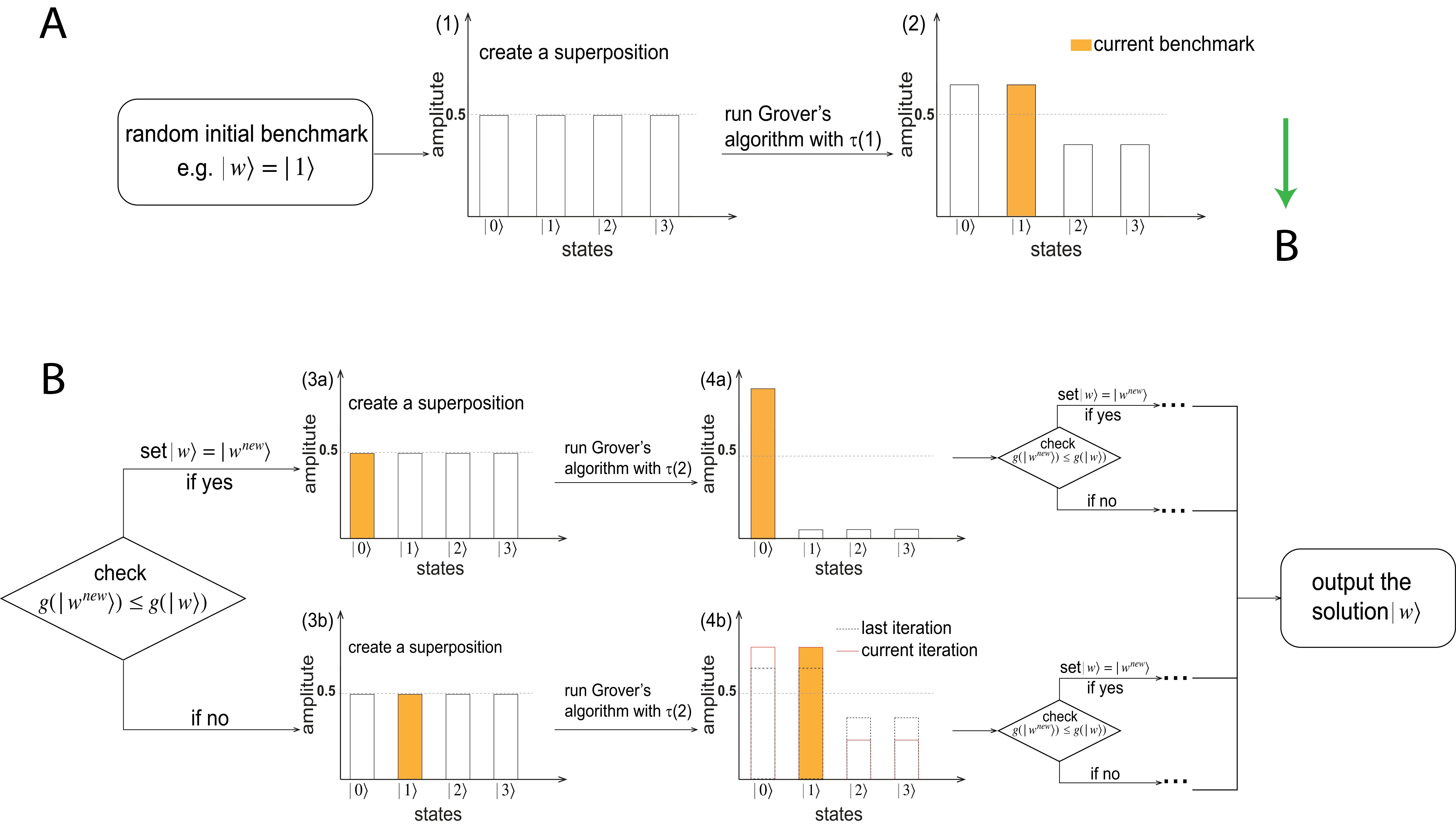
Figure 2: Illustrative example of quantum adaptive search.

3.3 Theoretical analysis of quantum adaptive search

Intuitively, one can think of QAS as a “quantum elevator” that starts at a random floor of a high tower and aims to descent to the ground floor. In each operation, a quantum machine will randomly decide if this elevator stays at the current floor or goes down to a random lower-level floor. Besides, the probability of going down will gradually increase as the number of operations increases. Thus, it is not hard to imagine that the “quantum elevator” can descent to the ground floor with a high success probability after a large enough amount of operations. Our intuition of QAS is justified by the following theorem. Theorem 3.1 states that within $O(\log_{2}D)$ iterations, QAS finds the sole solution state for any pre-specified success probability greater than 50%.

Theorem 3.1.

Let $\kappa\in(0.5,1)$ be a constant. With probability at least $\kappa$, the quantum adaptive search (e.g. Algorithm 2) finds the sole solution state $\ket{0}$ within $C_{\kappa}\log_{2}{D}$ iterations, where $C_{\kappa}$ is a positive constant that depends on $\kappa$.

Suppose that, in the $m$th iteration of Algorithm 2, the current benchmark state is $\ket{w_{m}}$ with $g(\ket{w_{m}}$ being the $r_{m}$th smallest among $\{g(\ket{i})\}_{i=0}^{D-1}$. Theorem 3.2 below shows the expected number of Grover’s operations that Algorithm 2 needs to update $g(\ket{w_{m}})$ is on the order $O(\sqrt{D/r_{m}})$. This together with Theorem 3.1 imply the computational complexity upper bound of QAS is of order $O(\sqrt{D}\log_{2}D)$ which is only a $\log_{2}D$ factor larger than the theoretical lower bound of any oracular quantum search algorithm (Bennett et al.,, 1997). Notice that, QAS achieves a near optimal computational efficiency as oracular quantum search algorithms without using any oracle information.

Theorem 3.2.

Let $\ket{w_{m}}$ be the current benchmark state in the $m$th iteration of Algorithm 2. Let $r_{m}$ be the rank of $g(\ket{w_{m}})$ in the sorted sequence of $\{g(\ket{i})\}_{i=0}^{D-1}$ in ascending order, $r_{m}\in\{1,\ldots,D\}$. The expected time for Algorithm 2 to update $\ket{w_{m}}$ is of order $O(\sqrt{D/r_{m}})$.

3.4 Computation of the loss function via quantum computing

The success of QAS relies on the efficient comparison of two states through the state loss function defined in (5), which is the MSE of linear regression. Recently, a line of studies (Wiebe et al.,, 2012; Rebentrost et al.,, 2014; Wang,, 2017; Zhao et al.,, 2019) focuses on formulating linear regression as a matrix inversion problem, which can be tackled by the quantum algorithm to solve linear systems of equations (Harrow et al.,, 2009). Their goal is to find a series of quantum states whose amplitudes represent the ordinary least squares estimator of linear regression coefficients. Although their algorithms can encode such quantum states efficiently, “it may be exponentially expensive to learn via tomography” (Harrow et al.,, 2009). As a result, most existing quantum linear regression algorithms require the input design matrix to be sparse. Otherwise, the computation is slow and the estimation accuracy may suffer from noise accumulation.

In this paper, we investigate a novel quantum linear prediction approach that is based on the singular-value decomposition. The proposed method avoids the matrix inversion problem. Instead, we estimate the inverse singular values by utilizing a recently developed quantum tomography technique (Lloyd et al.,, 2014). Let $\{j_{1},\ \ldots,\ j_{d}\}$ be a subset of $\{1,\ \ldots,\ p\}$ with $d\leq n$. Denote $\bm{X}_{d}\in\mathbb{R}^{n\times d}$ the sub-matrix of $\bm{X}$ corresponding to the subset $\{j_{1},\ \ldots,\ j_{d}\}$. Let $\widetilde{\bm{x}}$ be a new observation of the $d$ selected covariates. Then, the corresponding response value $\widetilde{y}$ can be predicted by

$$\widehat{y}=\widetilde{\bm{x}}^{\mathrm{\scriptstyle T}}(\bm{X}_{d}^{\mathrm{\scriptstyle T}}\bm{X}_{d})^{-1}\bm{X}_{d}^{\mathrm{\scriptstyle T}}\bm{y}.$$ (7)

Suppose that the rank of $\bm{X}_{d}$ is $R\leq d$, a compact singular value decomposition of $\bm{X}_{d}$ yields

$$\bm{X}_{d}=\bm{U}\bm{\Sigma}\bm{V}^{\mathrm{\scriptstyle T}}=\sum\limits_{r=1}^{R}\sigma_{r}\bm{u}_{r}\bm{v}_{r}^{\mathrm{\scriptstyle T}},$$

where $\bm{\Sigma}=\mathrm{diag}\{\sigma_{1},\ \ldots,\ \sigma_{R}\}$ is a diagonal matrix of $R$ positive singular values, and $\bm{U}=(\bm{u}_{1},\ \ldots,\ \bm{u}_{R})\in\mathbb{R}^{n\times R}$ and $\bm{V}=(\bm{v}_{1},\ \ldots,\ \bm{v}_{R})\in\mathbb{R}^{d\times R}$ are matrices of left and right singular vectors, respectively. Further, we have $\bm{U}\bm{U}^{\mathrm{\scriptstyle T}}=\bm{V}\bm{V}^{\mathrm{\scriptstyle T}}=\bm{I}_{R}$. Then, the linear predictor in (7) can be represented by

$$\widehat{y}=\sum\limits_{r=1}^{R}\sigma_{r}^{-1}\widetilde{\bm{x}}^{\mathrm{\scriptstyle T}}\bm{v}_{r}\bm{u}_{r}^{\mathrm{\scriptstyle T}}\bm{y}.$$ (8)

Motivated by the quantum principle component analysis (QPCA) (Lloyd et al.,, 2014) and the inverted singular value problem (Schuld et al.,, 2016), we propose to calculate (8) by a quantum linear prediction (QLP) procedure, which can be summarized as the following three steps.

Step 1: Quantum states preparation.

We encode $\bm{X}_{d}$, $\bm{v}_{r}$ and $\bm{u}_{r}$, $r=1,\ \ldots,\ R$, into a quantum system as

$$\ket{\bm{X}_{d}}=\sum_{j=1}^{d}\sum_{i=1}^{n}a_{i,j}\ket{i}\ket{j},\quad\ket{\bm{u}_{r}}=\sum\limits_{i=1}^{n}\mu_{r,i}\ket{i}\quad\text{and}\quad\ket{\bm{v}_{r}}=\sum\limits_{j=1}^{d}\nu_{r,j}\ket{j},$$ (9)

where $\sum_{i}\sum_{j}|a_{i,j}|^{2}=\sum_{i}|\mu_{r,i}|^{2}=\sum_{j}|\nu_{r,j}|^{2}=1$, and $\{\ket{i}\}_{i=1}^{n}$ and $\{\ket{j}\}_{j=1}^{d}$ are orthonormal quantum bases representing the linear space spanned by the left and right singular vectors of $\bm{X}_{d}$, respectively.

Then, we encode $\bm{X}_{d}^{\mathrm{\scriptstyle T}}\bm{X}_{d}$ and the compact singular value decomposition of $\bm{X}_{d}$ into a quantum system as

$${\mathbf{\rho}}\equiv{\mathbf{\rho}}(\bm{X}_{d}^{\mathrm{\scriptstyle T}}\bm{X}_{d})=\sum_{j,j^{\prime}=1}^{d}\sum_{i=1}^{n}a_{i,j}a_{i,j^{\prime}}\ket{j}\bra{j^{\prime}}\quad\text{and}\quad\ket{\bm{X}_{d}}=\sum\limits_{r=1}^{R}\sigma_{r}\ket{\bm{u}_{r}}\ket{\bm{v}_{r}}.$$ (10)

Similarly, we can encode $\bm{y}$ and $\widetilde{\bm{x}}$ into a quantum system as

$$\left|\mathbf{y}\right\rangle=\sum_{\eta=1}^{n}b_{\eta}\ket{\eta}\quad\text{and}\quad\ket{\widetilde{\bm{x}}}=\sum_{\gamma=1}^{d}c_{\gamma}\ket{\gamma},$$ (11)

with $\sum_{\eta}|b_{\eta}|^{2}=\sum_{\gamma}|c_{\gamma}|^{2}=1$, and $\{\ket{\eta}\}_{\eta=1}^{n}$ and $\{\ket{\gamma}\}_{\gamma=1}^{d}$ are orthonormal quantum bases.

Step 2: Extracting the inverted singular values.

To calculate (8) with a quantum computer, we first need to calculate the inverse of singular values of $\bm{X}_{d}$. According to the ideas of QPCA (Lloyd et al.,, 2014), we apply ${\mathbf{\rho}}$ to $\ket{{\bm{X}_{d}}}$ and follow the quantum phase estimation algorithm (e.g. Shor,, 1994; Szegedy,, 2004; Wocjan et al.,, 2009) which yields

$$\sum_{r=1}^{R}\sigma_{r}\ket{\bm{v}_{r}}\ket{\bm{u}_{r}}\ket{\lambda_{r}},$$ (12)

where $\lambda_{r}=\sigma_{r}^{2}$, $r=1,\ \ldots,\ R$, are the eigenvalues of ${\mathbf{\rho}}$ which is encoded in a quantum register $\ket{\lambda_{r}}$. Then, by adding an extra qubit and rotating (12) condition on the eigenvalue register $\ket{\lambda_{r}}$, we have

$$\sum_{r=1}^{R}\sigma_{r}\ket{\bm{v}_{r}}\ket{\bm{u}_{r}}\ket{\lambda_{r}}\left[\sqrt{1-(\frac{c}{\lambda_{r}})^{2}}\ket{0}+\frac{c}{\lambda_{r}}\ket{1}\right],$$ (13)

where $c$ is a constant to ensure the inverse of eigenvalues are no larger than 1.

We can repeatedly perform a conditional measurement of (13) until it is in state $\ket{1}$. After that, we can uncompute and discard the eigenvalue register which results in

$$\ket{\psi_{1}}\equiv\frac{1}{\sqrt{p(1)}}\sum_{r=1}^{R}\frac{c}{\sigma_{r}}\ket{\bm{v}_{r}}\ket{\bm{u}_{r}},$$ (14)

where $p(1)=\sum_{r=1}^{R}|\frac{c}{\lambda_{r}}|^{2}$ is the probability of the qubit in (13) collapsing to state $\ket{1}$.

Step 3: Calculating the inner products.

Follow the notations in (9) –(11), we can rewrite (8) as

$$\sum_{r=1}^{R}\sigma_{r}^{-1}\braket{\widetilde{\bm{x}}}{\bm{v}_{r}}\braket{\bm{y}}{\bm{u}_{r}}.$$ (15)

Motivated by the strategy in Schuld et al., (2016), we write (15) into some entries of a qubit so that it can be assessed by a single measurement. To this end, we construct two states $\ket{\psi_{1}}$ and $\ket{\psi_{2}}$ that are entangled with a qubit, i.e.

$$\frac{1}{\sqrt{2}}\left(\ket{\psi_{1}}\ket{0}+\ket{\psi_{2}}\ket{1}\right),$$

where $\ket{\psi_{1}}$ is defined in (14) and $\ket{\psi_{2}}=\ket{{\bm{y}}}\ket{{\widetilde{\bm{x}}}}$. Then, the off-diagonal elements of this qubit’s density matrix read

$$\frac{c}{2\sqrt{p(1)}}\sum_{r=1}^{R}\sigma_{r}^{-1}\braket{\widetilde{\bm{x}}}{\bm{v}_{r}}\braket{\bm{y}}{\bm{u}_{r}}=\frac{c}{2\sqrt{p(1)}}\sum_{r=1}^{R}\sigma_{r}^{-1}\widetilde{\bm{x}}^{\mathrm{\scriptstyle T}}\bm{v}_{r}\bm{u}_{r}^{\mathrm{\scriptstyle T}}{\bm{y}},$$

which contain the desired results (8) up to a known normalization factor.

Given a testing set of $n_{t}$ observations, i.e. $\{\widetilde{y}_{i},\widetilde{\bm{x}}_{i}\}_{i=1}^{n_{t}}$, the prediction error can be calculated as

$$\tilde{g}(\ket{i})=\frac{1}{n_{t}}\sum\limits_{i=1}^{n_{t}}(\widehat{y}_{i}-\widetilde{y}_{i})^{2},$$ (16)

where $\ket{i}$ is a quantum state represents $\{x_{1},\ \ldots\ ,x_{d}\}$ and $\widehat{y}_{i}$ is the predictor of $\widetilde{y}_{i}$ which can be calculated follow the QLP procedure introduced above. In addition, the computational complexity of running QLP over a training set of size $n$ and a testing set of $n_{t}$ is approximately of the order $O\left((n+n_{t})\log_{2}d\right)$ which is faster than the classical computing algorithm that is usually of order $O\left((n+n_{t})d\right)$.

4 Hybrid quantum adaptive search

Figure 3: Flowchart of hybrid quantum-classical strategy.

In the high dimensional regime, implementing the best subset selection procedure completely on a quantum computing system is desirable since both QAS and QLP are substantially faster than their classical counterparts. However, such an objective may not be readily accomplished due to the prototypical development of quantum computers. On one hand, the capacity of the state-of-the-art quantum processor (about 70 qubits) is still far from large enough to carry out big data applications. For example, the quantum state preparation step of QLP requires at least $2(\log_{2}d+\log_{2}n)$ qubits which may exceed the capacity of most public available quantum computers when $d$ and $n$ are moderate or large. On the other hand, existing quantum computing systems are usually highly sensitive to the environment and can be influenced by both internal and external noises (Sung et al.,, 2019). For example, a superconducting quantum computing system can be affected by the internal noises due to material impurities as well as the external noises that come from control electronics or stray magnetic fields (Kandala et al.,, 2019). Further, such noises can accumulate through the computing process and create a non-negligible bias.

To address the aforementioned practical challenges, we propose a hybrid quantum-classical strategy to balance computational efficiency, scalability, and reliability of quantum best subset selection. The intuition of the hybrid quantum-classical strategy is to advance complementary advantages of quantum and classical computing by implementing computational demanding steps on quantum nodes and running capacity demanding steps on classical nodes. The accuracy of quantum nodes can be boosted by some aggregation approaches, like majority voting. To be specific, we first input the data into a classical node and parallelly compute the linear prediction errors (16) over $D=2^{p}$ candidate models. The linear prediction errors, stored in a $D$-dimensional vector, will be passed to $K$ quantum nodes. Then, we independently implement QAS on $K$ quantum nodes to select the minimum element in the $D$-dimensional prediction error vector. The selection results, stored in a list of $K$ items, will be passed to a classical node for a majority voting. The best subset with the most votes is selected as the final estimator. We present the flow chart and details of this procedure in Figure 3 and Algorithm 3, respectively.

Algorithm 3 Hybrid quantum-classical strategy for best subset selection

Input: A training set $\{\bm{x}_{i},\ y_{i}\}_{i=1}^{n}$ with $\bm{x}_{i}\in\mathbb{R}^{p}$. A testing set $\{\widetilde{\bm{x}}_{i}\}_{i=1}^{n_{t}}$ with $\widetilde{\bm{x}}_{i}\in\mathbb{R}^{p}$. A number of available quantum nodes $K$. A learning rate $\lambda\in(0,1)$.

Stage 1 on a classical computer:

 (1.1) Compute, in parallel, the prediction error (16) over all $D=2^{p}$ candidate models.

 (1.2) Save the prediction errors $\bm{G}_{D}=\left(g(\ket{0}),\ \ldots,\ g(\ket{D-1})\right)$.

Stage 2 on $K$ quantum nodes:

 (2.1) Independently implement Algorithm 2 over $\bm{G}_{D}$ on $K$ quantum nodes.

 (2.2) Save the results in a list of $K$ selected models $\mathcal{M}=\{m_{1},\ \ldots,\ m_{K}\}$.

Stage 3 on a classical computer:

   A majority voting over models in $\mathcal{M}$. Denote the model with the most votes as $\widehat{m}$.

Output: The selected model $\widehat{m}$.

The Theorem 4.1 below states a majority voting over $K=2\xi+1$ independent quantum nodes can boost the success probability of finding the best subset. The lower bound of success probability in Theorem 4.1 can be boosted by increasing the number of quantum nodes or improving the success probability on each quantum node.

Theorem 4.1.

Let’s consider a majority voting system that consists of $K=2\xi+1$ nodes, where $\xi$ is a positive integer. Suppose that each node works independently with a probability $q>\frac{\xi+1}{2\xi+1}$ to vote the correct model and a probability $1-q$ to vote an incorrect model. Let $\cal E$ denote the event that the majority voting system selects the correct model. Then, the probability of $\cal E$ is lower bounded by

$$\mathbb{P}({\cal E})>\Phi\left(\sqrt{2(2\xi+1)D_{KL}(q,\frac{\xi+1}{2\xi+1})}\right),$$

where $\Phi(\cdot)$ is the cumulative distribution function of a standard normal random variable and

$$D_{KL}(a,b)=b\ln\frac{b}{a}+(1-b)\ln\frac{(1-b)}{(1-a)}$$

is the Kullback-Leibler divergence between two Bernoulli distributions with parameters $a$ and $b$, respectively.

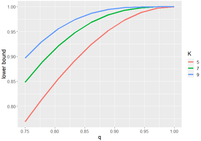
Figure 4: Lower bounds of successful probability when $K=5,7,9$.

In Figure 4, we plot the lower bound of $\mathbb{P}({\cal E})$ versus the values of $q$. We let $q$ increase from 0.75 to 1 and choose the number of nodes $K=5,7,9$. According to Figure 4, all three solid lines are concave curves which means a majority voting system with a moderate number of nodes can effectively boost the success probability of finding the correct model. For instance, a majority voting over $K=9$ independent nodes with $q=0.75$ can boost the probability of finding the correct model to 0.9 or higher.

5 Experiments on the quantum computer

In this section, we implement the proposed hybrid quantum-classical strategy on IBM Quantum Experience. This platform has developed a Qiskit Python development kit, which allows users to perform both quantum computing and classical computing in a single project. In Section 5.1, we analyze the performance of Algorithm 3 regarding the selections of tuning parameters. In Section 5.2, we assess the best subset section performance of Algorithm 3 under various linear regression settings and compare QAS with Grover’s algorithm in stage 2.

5.1 Selection of tuning parameters

The proposed hybrid quantum-classical strategy involves two tuning parameters: the number of quantum nodes $K$; and a learning rate $\lambda\in(0,1)$ which will be passed to each quantum node to implement Algorithm 2. As suggested by Theorem 4.1, the success probability of Algorithm 3 converges to 1 as $K$ increases when the success probability of each quantum node surpasses 0.5. Therefore, one should choose $K$ as large as possible subject to the availability of quantum computing resources. On the other hand, the learning rate $\lambda$ controls the “step size" of each iteration in Algorithm 2. In this subsection, we use an experiment to assess the performance and the sensitivity of Algorithm 3 with respect to the choices of $K$ and $\lambda$. To focus on the selection of tuning parameters, we skip the stage 1 in Algorithm 3. Instead, we generate $\bm{G}_{D}$ as an i.i.d. sample of size $D=32$ from the uniform distribution $U[0,1]$. Then we use the stages 2 and 3 in Algorithm 3 to find the minimum element in $\bm{G}_{D}$. We set $K=1$, $3$ or $5$, and let $\lambda$ be a sequence of grid points between 0.40 and 0.60 with a step size of 0.01. For each pair of $K$ and $\lambda$, we simulate 200 replications. The performance is measured by the accuracy rate which is defined as

$$\text{Accuracy rate}=\frac{\text{Number of replications with correct solution}}{\text{Number of replications}}.$$ (17)

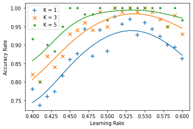
Figure 5: Accuracy rates of Algorithm 3 with $K=1,3,5$ and $\lambda\in[0.40,0.60]$.

The results are presented in Figure 5. The accuracy rates for $K=1,3$ or $5$ are plotted as blue, orange, and green dots with different symbols. The solid lines are corresponding smoothed curves. According to Figure 5, we find that increasing the number of quantum nodes $K$ can improve the accuracy rate though the improvement is marginal when $K$ is large enough, e.g. $K=5$. Besides, we observe that the highest accuracy rates are attained with some $\lambda$ between 0.5 and 0.55 for both choices of $K$. One can notice that the accuracy rates are close to 1 when $\lambda\in(0.5,0.55)$ and $K\geq 3$ which can be considered as a rule-of-thumb recommendation. Further, the smoothed curves in Figure 5 indicate that Algorithm 3 is not very sensitive for the selection of tuning parameters.

5.2 Best subset selection with hybrid quantum-classical strategy

In this subsection, we assess the best subset selection performance of the proposed hybrid quantum-classical strategy. We consider a linear regression model

$$y_{i}=\bm{x}_{i}^{\mathrm{\scriptstyle T}}\bm{\beta}^{\ast}+\epsilon_{i},\quad i=1,\ \ldots,\ n,$$ (18)

where $y_{i}\in\mathbb{R}$, $\bm{x}_{i}\in\mathbb{R}^{p}$, $\bm{\beta}^{\ast}=(\beta_{1},\ \ldots\ ,\beta_{p})^{\mathrm{\scriptstyle T}}\in\mathbb{R}^{p}$, and $\epsilon_{i}\in\mathbb{R}$. First, we draw $\{\bm{x}_{i}\}_{i=1}^{n}$ as an i.i.d. sample from a multivariate normal distribution $N_{p}({\bf 0},\bm{\Sigma})$, where the $(i,j)$th entry of $\bm{\Sigma}$ equals $\rho^{|i-j|}$ for some $\rho\in(0,1)$. Then, we draw $\{\epsilon_{i}\}_{i=1}^{n}$ as an i.i.d. sample from a normal distribution $N(0,\sigma^{2})$. Notice that, $\rho$ controls the autocorrelation level among covariates, and $\bm{\beta}^{\ast}$, $\rho$ and $\sigma$ together control the signal to noise ratio (SNR), i.e. $\text{SNR}=\bm{\beta}^{\ast\mathrm{\scriptstyle T}}\bm{\Sigma}\bm{\beta}^{\ast}/\sigma^{2}$. Let $s<p$ be a positive integer indicating the model sparsity. We set the first $s$ elements of $\bm{\beta}^{\ast}$ to be 1 and the rest $p-s$ elements to be 0.

Subject to the capacity of the quantum computing system, we set $n=100$, $p=7$, and $s=4$. We choose the autocorrelation level $\rho\in\{0.25,0.5\}$ and the signal to noise ratio $\text{SNR}\in\{0.5,1.0,2.0,3.0\}$, respectively. For each scenario, we simulate 200 replications. We implement the hybrid quantum-classical strategy as proposed in Algorithm 3 with $K=3$ and $\lambda=0.55$ to select the best subset of the linear regression model. We denote this method as QAS since it implements the quantum adaptive search in stage 2. Besides, we consider two variants of Algorithm 3 as two competitors. The first competitor, denoted as Grover Oracle, replaces QAS in stage 2 by Grover’s algorithm with a known oracle state. The second competitor, denoted as Grover Random, replaces QAS in stage 2 by Grover’s algorithm with a randomly selected oracle state. Notice that Grover Oracle is an oracular method and not applicable in practice since the oracle state is not observable.

For each replication, we record the false positives (FP) and false negatives (FN) of each method. FP is the number of inactive covariates that are selected into the model and FN is the number of active covariates that are ignored in the selected model. The box-plots of FP and FN over 200 replications are reported in Figure 6 below. According to Figure 6, Grover Oracle performs the best among the three competitors which is not surprising as it utilizes the oracle information of the true best subset. The proposed QAS method, as a non-oracular approach, performs almost identical to Grover Oracle in nearly all scenarios. QAS is slightly outperformed by Grover Oracle when the correlation level is high ($\rho=0.5$) and the signal to noise ratio is small ($\text{SNR}=0.5$), which is the most challenging scenario. In contrast, Grover Random performs as bad as random guesses in all scenarios. This observation, which is inline with the discussions in Section 2.2.3, shows oracular quantum search algorithms are not suitable to statistical learning problems.

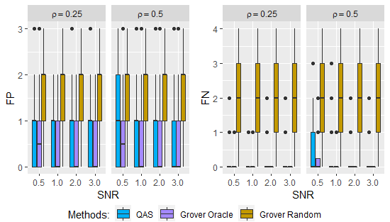
Figure 6: Box-plots of false positives (left) and false negatives (right) over 200 replications.

6 Comparison with classical methods

In this section, we compare the empirical performance of quantum adaptive search (QAS) with the naive best subset selection method (BSS) implemented on a classical computer. We also include some popular approximate best subset selection methods designed for classical computers: forward stepwise selection (e.g. Draper and Smith,, 1966); LASSO (Tibshirani,, 1996); and the fast best subset selection method (L0Learn) (Hazimeh and Mazumder,, 2018). The implementation details of the 5 comparison methods are summarized in Table 1.

Table 1: Implementation details for the 5 comparison methods in Section 6.

Method name		Computing method		Tuning parameter selection
QAS		Algorithm 3		$K=5$ and $\lambda=0.5$
BSS		Naive best subset selection		NA
Forward stepwise		R package bestsubset		NA
LASSO		R package glmnet		10-folds cross-validation
L0Learn		R package L0Learn		10-folds cross-validation

We consider the same linear regression model in (18). The coefficient vector $\bm{\beta}^{\ast}$ is generated from one of the following two settings.

• Strong sparsity: the first $s$ elements of $\beta^{*}$ equal to 1 while the rest $p-s$ elements equal to 0.

• Weak sparsity: the first $s$ elements of $\beta^{*}$ equal to $1,\frac{s-1}{s},\frac{s-2}{s},\ \ldots,\ \frac{1}{s}$ while the rest $p-s$ elements equal to 0.

In this experiment, we set $n=100$, $p=10$ and $s=5$. We choose the autocorrelation level $\rho\in\{0.25,0.5\}$ and the signal to noise ratio $\text{SNR}\in\{0.5,1.0,2.0,3.0\}$, respectively. For each scenario, we simulate 100 replications. Additional results for $p=20$ and a real data analysis are relegated to the supplemental material. Besides the false positives (FP) and false negatives (FN) defined in Section 5.2, we measure the prediction performance of each method by the relative test error (RTE):

$$\text{RTE}=\mathbb{E}(\widetilde{y}-\widetilde{\bm{x}}^{T}\widehat{\bm{\beta}})^{2}/\sigma^{2}=(\widehat{\bm{\beta}}-\bm{\beta}^{\ast})^{\mathrm{\scriptstyle T}}\bm{\Sigma}(\widehat{\bm{\beta}}-\bm{\beta}^{\ast})/\sigma^{2}+1,$$

where $(\tilde{y},\tilde{\bm{x}})$ is a testing observation which is i.i.d. with the training sample $\{y_{i},\bm{x}_{i}\}_{i=1}^{n}$. It is easy to see that RTE is lower bounded by 1 and the smaller the better.

Figures 7 and 8 present box-plots of FP, FN and RTE over 100 replications under strong sparsity and weak sparsity settings, respectively. According to the box-plots, none of the 5 competing methods dominate the others in terms of all three measurements, which is inline with the discussions in Hastie et al., (2020). Generally speaking, LASSO tends to select generous models which may have small FNs but large FPs. Forward stepwise and L0Learn prefer to select parsimonious models which may lead to small FPs but large FNs. However, none of the three methods can be considered as a good approximation of BSS since their performance are distinct in most scenarios. In contrast, QAS performs almost identical to BSS in terms of all three measurements in every scenario.

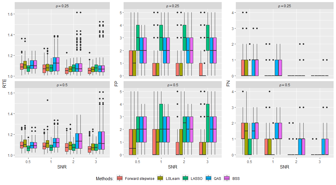
Figure 7: Strong sparsity setting: Boxplots of relative test error (left), false positives (middle) and false negatives (right) over 100 replications.

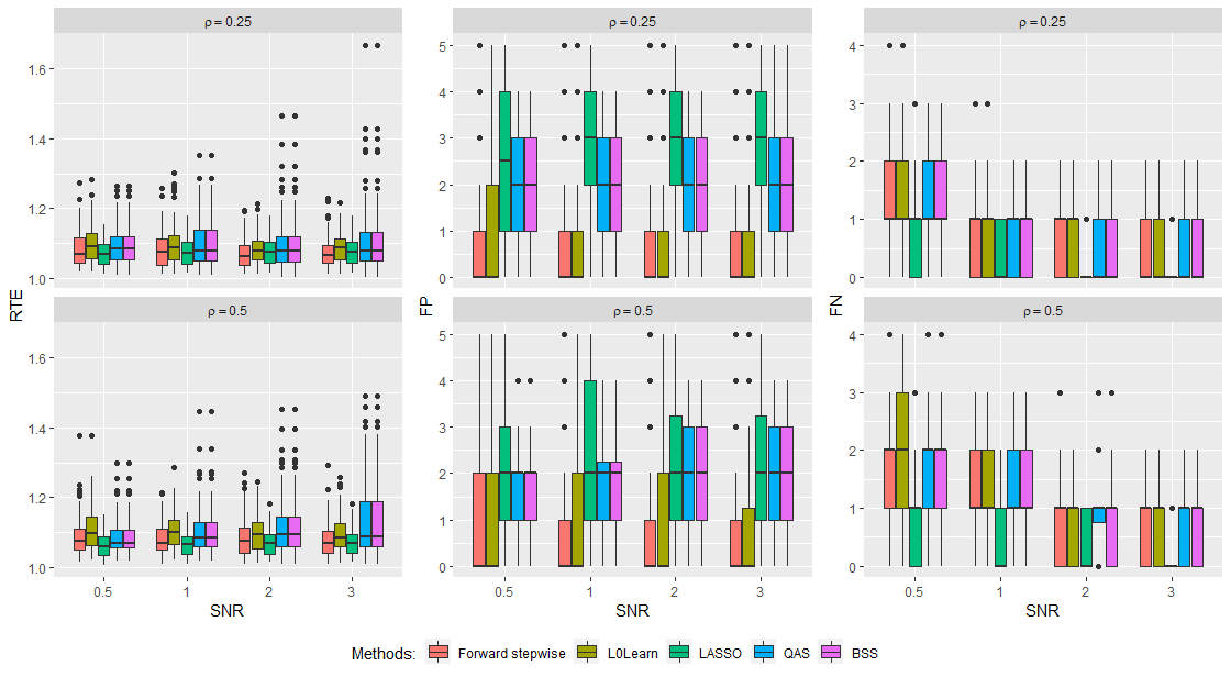
Figure 8: Weak sparsity setting: Boxplots of relative test error (left), false positives (middle) and false negatives (right) over 100 replications.

Next, we take a closer look at best subset selection behaviors of the 5 comparison methods. We simulate 1,000 replications of (18) with $n=100$, $p=10$, $s=5$, $\rho=0.5$, $\text{SNR}=0.5$, and the strong sparsity $\bm{\beta}^{*}$. In the top panel of Figure 9, we present the histogram of selected model sizes for 5 methods. In the bottom panel of Figure 9, we report the box-plots of RTSs for 5 methods. According to Figure 9, the selected model sizes of QAS and BSS sharply concentrates around the truth, i.e. $s=5$. The histograms of Forward stepwise and L0Learn are severely left skewed which indicates they tend to underestimate the size of the active set. In contrast, LASSO has a right skewed histogram and hence often select oversized models. Again, the selection as well as prediction performances of QAS and BSS are almost identical. The results in Figure 9 further justified our argument that QAS is an efficient quantum alternative of BSS while Forward stepwise, LASSO and L0Learn are not ideal approximates of BSS.

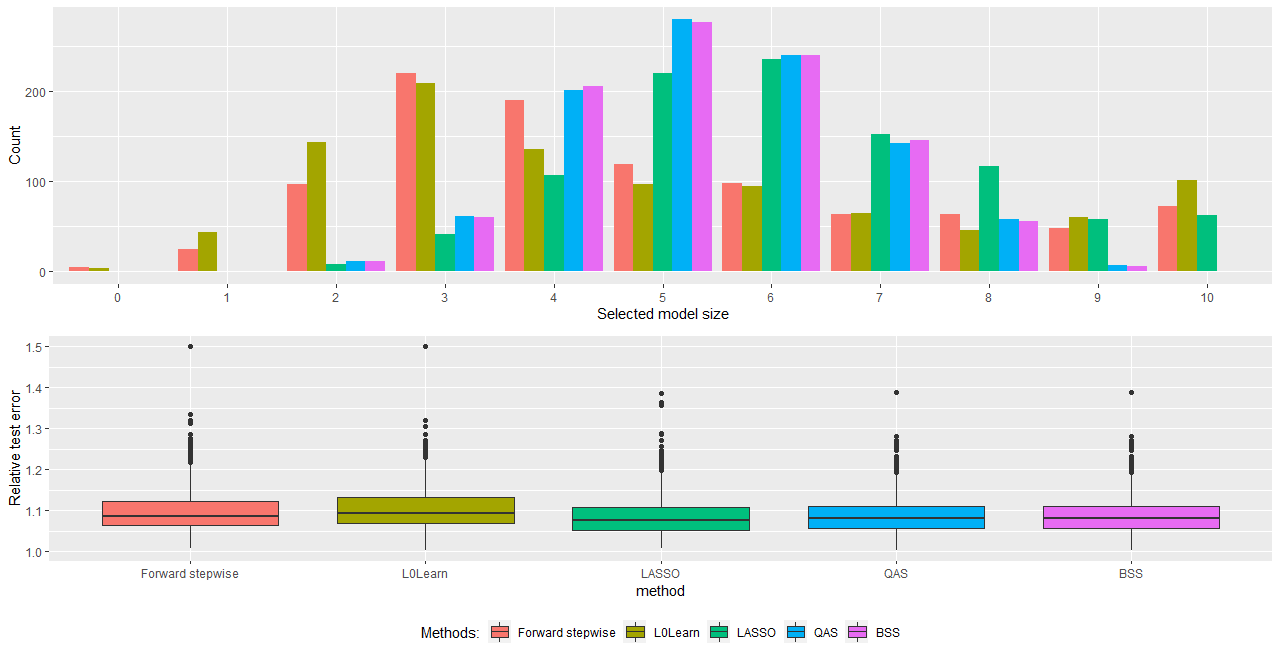
Figure 9: Best subset selection behaviors: histogram of selected model size (top) and boxplots of relative test error (bottom).

7 Conclusion

In this paper, we investigated the solution of the best subset selection problem in a quantum computing system. We proposed an adaptive quantum search algorithm that does not require the oracle information of the solution state and can significantly reduce the computational complexity of classical best subset selection methods. An efficient quantum linear prediction method was also discussed. Further, we introduced a novel hybrid quantum-classical strategy to avoid the hardware bottleneck of existing quantum computing systems and boost the success probability of quantum adaptive search. The quantum adaptive search is applicable to various best subset selection problems. Moreover, our study opens the door to a new research area: reinvigorating statistical learning with powerful quantum computers.

References

- Abrams and Lloyd, (1997) Abrams, D. S. and Lloyd, S. (1997). Simulation of many-body fermi systems on a universal quantum computer. Physical Review Letters, 79(13):2586.
- Beale et al., (1967) Beale, E., Kendall, M., and Mann, D. (1967). The discarding of variables in multivariate analysis. Biometrika, 54(3-4):357–366.
- Bennett et al., (1997) Bennett, C. H., Bernstein, E., Brassard, G., and Vazirani, U. (1997). Strengths and weaknesses of quantum computing. SIAM journal on Computing, 26(5):1510–1523.
- Bertsimas et al., (2016) Bertsimas, D., King, A., and Mazumder, R. (2016). Best subset selection via a modern optimization lens. The Annals of Statistics, 44(2):813–852.
- Boyer et al., (1998) Boyer, M., Brassard, G., Høyer, P., and Tapp, A. (1998). Tight bounds on quantum searching. Fortschritte der Physik: Progress of Physics, 46(4-5):493–505.
- Breiman, (1996) Breiman, L. (1996). Heuristics of instability and stabilization in model selection. The Annals of Statistics, 24(6):2350–2383.
- Byrnes and Yamamoto, (2006) Byrnes, T. and Yamamoto, Y. (2006). Simulating lattice gauge theories on a quantum computer. Physical Review A, 73(2):022328.
- Candes and Tao, (2007) Candes, E. and Tao, T. (2007). The dantzig selector: Statistical estimation when p is much larger than n. The Annals of Statistics, 35(6):2313–2351.
- Chen and Donoho, (1994) Chen, S. and Donoho, D. (1994). Basis pursuit. In Proceedings of 1994 28th Asilomar Conference on Signals, Systems and Computers, volume 1, pages 41–44. IEEE.
- Draper and Smith, (1966) Draper, N. and Smith, H. (1966). Applied regression analysis. j. wiley & sons inc., ny.
- Efroymson, (1960) Efroymson, M. (1960). Multiple regression analysis. Mathematical methods for digital computers, pages 191–203.
- Fan et al., (2020) Fan, J., Guo, Y., and Zhu, Z. (2020). When is best subset selection the "best"?
- Fan and Li, (2001) Fan, J. and Li, R. (2001). Variable selection via nonconcave penalized likelihood and its oracle properties. Journal of the American Statistical Association, 96(456):1348–1360.
- Fan et al., (2014) Fan, J., Xue, L., and Zou, H. (2014). Strong oracle optimality of folded concave penalized estimation. The Annals of Statistics, 42(3):819.
- Grover, (1997) Grover, L. K. (1997). Quantum mechanics helps in searching for a needle in a haystack. Physical Review Letters, 79(2):325.
- Hallgren, (2002) Hallgren, S. (2002). Polynomial-time quantum algorithms for pell’s equation and the principal ideal problem. In Proceedings of the thiry-fourth annual ACM symposium on Theory of computing, pages 653–658.
- Harrow et al., (2009) Harrow, A. W., Hassidim, A., and Lloyd, S. (2009). Quantum algorithm for linear systems of equations. Physical Review Letters, 103(15):150502.
- Hastie et al., (2020) Hastie, T., Tibshirani, R., and Tibshirani, R. (2020). Best subset, forward stepwise or lasso? analysis and recommendations based on extensive comparisons. Statistical Science, 35:579–592.
- Hazimeh and Mazumder, (2018) Hazimeh, H. and Mazumder, R. (2018). Fast best subset selection: Coordinate descent and local combinatorial optimization algorithms. Operations Research, 68.
- Hocking and Leslie, (1967) Hocking, R. and Leslie, R. (1967). Selection of the best subset in regression analysis. Technometrics, 9(4):531–540.
- Hu and Wang, (2020) Hu, J. and Wang, Y. (2020). Quantum annealing via path-integral monte carlo with data augmentation. Journal of Computational and Graphical Statistics, pages 1–13.
- Jansen et al., (2007) Jansen, S., Ruskai, M.-B., and Seiler, R. (2007). Bounds for the adiabatic approximation with applications to quantum computation. Journal of Mathematical Physics, 48(10):102111.
- Jordan, (2005) Jordan, S. P. (2005). Fast quantum algorithm for numerical gradient estimation. Physical Review Letters, 95(5):050501.
- Kandala et al., (2019) Kandala, A., Temme, K., Córcoles, A. D., Mezzacapo, A., Chow, J. M., and Gambetta, J. M. (2019). Error mitigation extends the computational reach of a noisy quantum processor. Nature, 567(7749):491–495.
- Kassal et al., (2008) Kassal, I., Jordan, S. P., Love, P. J., Mohseni, M., and Aspuru-Guzik, A. (2008). Polynomial-time quantum algorithm for the simulation of chemical dynamics. Proceedings of the National Academy of Sciences, 105(48):18681–18686.
- Lloyd et al., (2014) Lloyd, S., Mohseni, M., and Rebentrost, P. (2014). Quantum principal component analysis. Nature Physics, 10(9):631–633.
- Natarajan, (1995) Natarajan, B. K. (1995). Sparse approximate solutions to linear systems. SIAM journal on computing, 24(2):227–234.
- Nielsen and Chuang, (2010) Nielsen, M. A. and Chuang, I. L. (2010). Quantum Computation and Quantum Information. Cambridge University Press.
- Rebentrost et al., (2014) Rebentrost, P., Mohseni, M., and Lloyd, S. (2014). Quantum support vector machine for big data classification. Physical Review Letters, 113(13):130503.
- Schuld and Petruccione, (2018) Schuld, M. and Petruccione, F. (2018). Supervised Learning with Quantum Computers. Springer.
- Schuld et al., (2016) Schuld, M., Sinayskiy, I., and Petruccione, F. (2016). Prediction by linear regression on a quantum computer. Physical Review A, 94(2):022342.
- Shen et al., (2012) Shen, X., Pan, W., and Zhu, Y. (2012). Likelihood-based selection and sharp parameter estimation. Journal of the American Statistical Association, 107(497):223–232.
- Shor, (1994) Shor, P. W. (1994). Algorithms for quantum computation: discrete logarithms and factoring. In Proceedings 35th annual symposium on foundations of computer science, pages 124–134. IEEE.
- Shor, (1999) Shor, P. W. (1999). Polynomial-time algorithms for prime factorization and discrete logarithms on a quantum computer. SIAM review, 41(2):303–332.
- Sung et al., (2019) Sung, Y., Beaudoin, F., Norris, L. M., Yan, F., Kim, D. K., Qiu, J. Y., von Lüpke, U., Yoder, J. L., Orlando, T. P., Gustavsson, S., et al. (2019). Non-gaussian noise spectroscopy with a superconducting qubit sensor. Nature Communications, 10(1):1–8.
- Szegedy, (2004) Szegedy, M. (2004). Quantum speed-up of markov chain based algorithms. In 45th Annual IEEE symposium on foundations of computer science, pages 32–41. IEEE.
- Tibshirani, (1996) Tibshirani, R. (1996). Regression shrinkage and selection via the lasso. Journal of the Royal Statistical Society: Series B (Methodological), 58(1):267–288.
- Van Dam and Shparlinski, (2008) Van Dam, W. and Shparlinski, I. E. (2008). Classical and quantum algorithms for exponential congruences. In Workshop on Quantum Computation, Communication, and Cryptography, pages 1–10. Springer.
- Wang, (2017) Wang, G. (2017). Quantum algorithm for linear regression. Physical review A, 96(1):012335.
- Wang, (2011) Wang, Y. (2011). Quantum monte carlo simulation. The Annals of Applied Statistics, 5(2A):669–683.
- Welch, (1982) Welch, W. J. (1982). Algorithmic complexity: three np-hard problems in computational statistics. Journal of Statistical Computation and Simulation, 15(1):17–25.
- Wiebe et al., (2012) Wiebe, N., Braun, D., and Lloyd, S. (2012). Quantum algorithm for data fitting. Physical Review Letters, 109(5):050505.
- Wocjan et al., (2009) Wocjan, P., Chiang, C.-F., Nagaj, D., and Abeyesinghe, A. (2009). Quantum algorithm for approximating partition functions. Physical Review A, 80(2):022340.
- Yuan and Lin, (2007) Yuan, M. and Lin, Y. (2007). On the non-negative garrotte estimator. Journal of the Royal Statistical Society: Series B (Statistical Methodology), 69(2):143–161.
- Zhang, (2010) Zhang, C.-H. (2010). Nearly unbiased variable selection under minimax concave penalty. The Annals of Statistics, 38(2):894–942.
- Zhao and Yu, (2006) Zhao, P. and Yu, B. (2006). On model selection consistency of lasso. Journal of Machine learning research, 7(Nov):2541–2563.
- Zhao et al., (2019) Zhao, Z., Fitzsimons, J. K., and Fitzsimons, J. F. (2019). Quantum-assisted gaussian process regression. Physical Review A, 99(5):052331.
- Zou, (2006) Zou, H. (2006). The adaptive lasso and its oracle properties. Journal of the American Statistical Association, 101(476):1418–1429.
- Zou and Hastie, (2005) Zou, H. and Hastie, T. (2005). Regularization and variable selection via the elastic net. Journal of the Royal Statistical Society: Series B (statistical methodology), 67(2):301–320.