We investigate the relationship between shadow radius and microstructure for a general static spherically symmetric black hole and confirm their close connection. In this regard, we take the Reissner-Nordström (AdS) black hole as an example to do the concrete analysis. On the other hand, we study for the Kerr (AdS) black hole the relationship between its shadow and thermodynamics in the aspects of phase transition and microstructure. Our results for the Kerr (AdS) black hole show that the shadow radius $r_{\rm sh}$, the deformation parameters $\delta_{s}$ and $k_{s}$, and the circularity deviation $\Delta C$ can reflect the black hole thermodynamics. In addition, we give the constraints to the relaxation time of the M$87^{*}$ black hole by combining its shadow data and the Bekenstein-Hod universal bounds when the M$87^{*}$ is regarded as the Reissner-Nordström or Kerr black hole. We predict that the minimum relaxation times of M$87^{*}$ black hole and Sgr $A^{*}$ black hole are approximately 3 days and 2.64 minutes, respectively. Finally, we draw the first graph of the minimum relaxation time $\tau_{\rm min}$ with respect to the maximum shadow radius $r_{\rm sh}^{\rm max}$ at different mass levels.

1 Introduction

Recently, the Event Horizon Telescope (EHT) collaboration has released [1, 2] for the first time the shadow image of the supermassive black hole in the center of M8$7^{*}$ galaxy, which greatly stimulates our enthusiasm for the research of black hole shadows. The essence of shadows is that the specific photons around a black hole collapse inward to form a dark area observed by a distant observer, which shows that the shadow appears to be a dynamical phenomenon of black holes. Through black hole shadows, one not only obtains [3, 4, 5, 6, 7] the mass, spin, charge, and other information of black holes, but also knows [8, 9, 10, 11] the distribution of matter around black holes. More importantly, the relevant research opens a new window for us to study the strong gravitational region near black hole horizons. So far, there have been a large number of articles on black hole shadows under Einstein gravity and modified gravity theories, see, for instance, some literature [12, 13, 14, 15, 16, 17, 18, 19, 20, 21, 22, 23, 24, 25, 26, 27, 28, 29, 30, 31, 32, 33, 34, 35, 36, 37, 38, 39, 40, 41, 42, 43, 44, 45, 46, 47, 48, 49, 50, 51, 52, 53].

A shadow is an observable quantity which is potentially related to black hole thermodynamics. As is known, the black hole thermodynamics [54, 55, 56, 57, 58] is an important subject of black hole physics, especially when combined with AdS spacetimes, the black hole thermodynamics in extended phase spaces has achieved great progress, e.g., the van der Waals-like phase transition occurs [59, 60, 61, 62, 63] in the Reissner-Nordstr$\mathrm{\ddot{o}}$m AdS black hole, the reentrant phase transition happens [64] in high-dimensional rotating black holes, and so on. Now black holes are not only regarded as a strong gravitational system, but also as a thermodynamic one, so it is necessary to explore the relationship between its dynamics and thermodynamics. Recently, the relationships between dynamic characteristic quantities and thermodynamic ones have been studied [65, 66, 67, 68, 69, 70, 71, 72, 73, 74]. Some results show [65, 66] that the unstable circular orbital motion can connect thermodynamic phase transitions of black holes. For a static spherically symmetric black hole, its timelike or lightlike circular orbital motion of a test particle and its shadow indeed have a close connection [68, 73, 74] to its thermodynamic phase transition. Moreover, for a rotating black hole with the cosmological constant its shadow radius can also reflect [73] its thermodynamic phase transition.

The Ruppeiner thermodynamic geometry [75, 76, 77, 78] is a useful tool to study black hole thermodynamics. It provides [79, 80, 81, 82, 83, 84, 85, 86, 87, 88, 89, 90, 91, 92, 93] helpful information about microstructure of black holes. Its most important physical quantity is the Ruppeiner thermodynamic scalar curvature. It has been shown [76, 78, 84, 87, 88, 89] that this scalar curvature can take a positive, or a negative, or a vanishing value which corresponds to a repulsive, or an attractive, or no interaction among black hole molecules, respectively. As is known, the black hole microstructure represents an important aspect of black hole thermodynamics. Therefore, it is necessary to associate a shadow radius with the Ruppeiner thermodynamic scalar curvature, so as to connect such an observable to black hole microstructure.

We emphasize our main motivation: Considering that the thermodynamic phase transition and microstructure of black holes are not detectable directly, we want to connect certain observables that describe the characteristics of shadow deformations of rotating black holes to the two aspects of black hole thermodynamics, thus taking a glimpse of the inside of a black hole from the outside. Our investigations may provide some helps for understanding black hole thermodynamics via black hole shadows.

The paper is organized as follows. In Sec. 2, we investigate the relationship between shadow radius and microstructure for a general static spherically symmetric black hole. Then, we take Reissner-Nordström (AdS) black hole as an example to do the concrete analysis in Sec. 3. We study the relationship between shadow and thermodynamics in the aspects of phase transition and microstructure for the Kerr (AdS) black hole in Sec. 4. We give in Sec. 5 the constraints to the relaxation time of black hole perturbation based on shadow data. Finally, we make a summary in Sec. 6. We use the units $c=G=k_{\rm B}=\hbar=1$ and the sign convention $(-,+,+,+)$ throughout this paper.

2 Relationship between shadow radius and microstructure for a static spherically symmetric black hole

A general static spherically symmetric black hole can be described by the line element,

$$ds^{2}=-f(r)dt^{2}+\frac{dr^{2}}{g(r)}+r^{2}\left(d\theta^{2}+\sin^{2}\theta d\varphi^{2}\right),$$ (1)

where $f(r)$ and $g(r)$ are functions of radial coordinate $r$. The Hamilton-Jacobi equation can be used to separate the null geodesic equations in the spacetime of static spherically symmetric black holes and the general expression of shadows can be derived for this class of black holes. The Hamilton-Jacobi equation takes [94] the form,

$$\frac{\partial{\cal S}}{\partial\lambda}+{\cal H}=0,\qquad{\cal H}=\frac{1}{2}g_{\mu\nu}p^{\mu}p^{\nu},$$ (2)

where $\lambda$ is the affine parameter of null geodesics, ${\cal S}$ the Jacobi action, ${\cal H}$ the Hamiltonian, and the momentum $p^{\mu}$ is defined by

$$p_{\mu}\equiv\frac{\partial{\cal S}}{\partial x^{\mu}}=g_{\mu\nu}\frac{\mathrm{d}x^{\nu}}{\mathrm{d}\lambda}.$$ (3)

Due to the spherical symmetry of Eq. (1), without loss of generality, one can consider the photons moving on the equatorial plane with $\theta=\frac{\pi}{2}$. So the the Jacobi action ${\cal S}$ can be decomposed into the following form,

$${\cal S}=\frac{1}{2}m^{2}\lambda-Et+L\varphi+S_{r}(r),$$ (4)

where $m$ is the mass of moving particles around a static spherically symmetric black hole ($m=0$ for photons), $E$ the energy of photons, $L$ the angular momentum of photons, and $S_{r}(r)$ a function of coordinate $r$. By substituting Eqs. (1), (3) and (4) into Eq. (2), one can get the following three equations describing the motion of photons on the equatorial plane,

$$\frac{\mathrm{d}t}{\mathrm{d}\lambda} = \frac{E}{f(r)},$$ (5)

$$\frac{\mathrm{d}r}{\mathrm{d}\lambda} = \pm\frac{\sqrt{g(r)}}{\sqrt{f(r)}}\frac{\sqrt{E^{2}r^{4}-L^{2}r^{2}f(r)}}{r^{2}},$$ (6)

$$\frac{\mathrm{d}\varphi}{\mathrm{d}\lambda} = \frac{L}{r^{2}}.$$ (7)

Combining Eq. (6) with Eq. (7), one has

$$\frac{\mathrm{d}r}{\mathrm{d}\varphi}=\frac{\frac{\mathrm{d}r}{\mathrm{d}\lambda}}{\frac{\mathrm{d\varphi}}{\mathrm{d}\lambda}}=\pm r\sqrt{g(r)\left(\frac{r^{2}E^{2}}{L^{2}f(r)}-1\right)}.$$ (8)

Again considering $\left.\frac{\mathrm{d}r}{\mathrm{d}\varphi}\right|_{r=\xi}=0$ at the turning point of photon orbits, one can rewrite Eq. (8) as

$$\frac{\mathrm{d}r}{\mathrm{d}\varphi}=\pm r\sqrt{g(r)\left(\frac{r^{2}f(\xi)}{\xi^{2}f(r)}-1\right)}.$$ (9)

In addition, according to the equation satisfied by the effective potential $V(r)$,

$$\left(\frac{\mathrm{d}r}{\mathrm{d}\lambda}\right)^{2}+V(r)=0,$$ (10)

one obtains

$$V(r)=g(r)\left(\frac{L^{2}}{r^{2}}-\frac{E^{2}}{f(r)}\right).$$ (11)

Using the effective potential, one can determine [94] the critical orbit radius of photons, i.e. the photosphere radius in a static spherically symmetric spacetime,

$$V(r)=0,\qquad\frac{\mathrm{d}V(r)}{\mathrm{d}r}=0,\qquad\frac{d^{2}V(r)}{dr^{2}}<0.$$ (12)

By substituting Eq. (11) into Eq. (12), one can obtain the following relationships,

$$\frac{L^{2}}{E^{2}}=\frac{r^{2}_{\rm p}}{f(r_{\rm p})},$$ (13)

$$r\frac{\mathrm{d}f(r)}{\mathrm{d}r}-2f(r)\bigg{|}_{r=r_{\rm p}}=0,$$ (14)

where $r_{\rm p}$ is the radius of photospheres.

Considering that the light emitted from a static observer at position $r_{0}$ transmits into the past with an angle $\vartheta$ relative to the radial direction, one obtains [21, 22, 73]

$$\cot\vartheta=\frac{\sqrt{g_{rr}}}{\sqrt{g_{\varphi\varphi}}}\frac{\mathrm{d}r}{\mathrm{d}\varphi}\bigg{|}_{r=r_{0}}=\pm\sqrt{\frac{{r_{0}}^{2}f(\xi)}{\xi^{2}f(r_{0})}-1}.$$ (15)

When the relation $\sin^{2}\vartheta=\frac{1}{1+\cot^{2}\vartheta}$ is used, the above equation can be written as

$$\sin^{2}\vartheta=\frac{{\xi}^{2}f(r_{0})}{{r_{0}}^{2}f(\xi)}.$$ (16)

Therefore, the shadow radius of black holes observed by a static observer at position $r_{0}$ can be expressed [11, 21, 22, 73] by

$$r_{\rm sh}\equiv r_{0}\sin\vartheta=\left.\xi\sqrt{\frac{f(r_{0})}{f(\xi)}}\right|_{\xi\rightarrow r_{\rm p}}.$$ (17)

In the Ruppeiner thermodynamic geometry, the most important physical quantity that describes the microstructure of black holes is the Ruppeiner thermodynamic scalar curvature $R$ [75, 76]. If the entropy representation is chosen [95, 96, 97], this scalar curvature can be expressed by a function of event horizon radius and the other parameters,

$$R(S,...)=R(S(r_{\rm H}),...),$$ (18)

which leads to

$$\frac{\partial R}{\partial r_{\rm H}}=\frac{\partial R}{\partial r_{\rm sh}}\frac{\mathrm{d}r_{\rm sh}}{\mathrm{d}r_{\rm H}}.$$ (19)

As a result, according to the relation [68, 73],

$$\frac{\mathrm{d}r_{\rm sh}}{\mathrm{d}r_{\rm H}}>0,$$ (20)

we know that the conditions

$$\frac{\partial R}{\partial r_{\rm H}}>0,\qquad\frac{\partial R}{\partial r_{\rm H}}=0,\qquad\frac{\partial R}{\partial r_{\rm H}}<0,$$ (21)

can be converted to

$$\frac{\partial R}{\partial r_{\rm sh}}>0,\qquad\frac{\partial R}{\partial r_{\rm sh}}=0,\qquad\frac{\partial R}{\partial r_{\rm sh}}<0.$$ (22)

We thus establish the relationship between shadow radius and microstructure for a general static spherically symmetric black hole. Next, we take the Reissner-Nordstr$\mathrm{\ddot{o}}$m (RN) AdS black hole as an example to analyze the connection between Ruppeiner thermodynamic scalar curvature and shadow radius.

3 Relationship between shadow and microstructure for RN (AdS) black holes

The line element of the RN AdS black hole is given by [57, 59]

$$ds^{2}=-f(r)dt^{2}+\frac{dr^{2}}{f(r)}+r^{2}\left(d\theta^{2}+\sin^{2}\theta d\varphi^{2}\right),$$ (23)

with

$$f(r)=1-\frac{2M}{r}+\frac{q^{2}}{r^{2}}-\frac{\Lambda r^{2}}{3}.$$ (24)

Here $M$ is the black hole mass, $q$ the charge, $\Lambda$ the negative cosmological constant. In the extended phase space including the cosmological constant, some thermodynamic quantities for the RN AdS black hole are as follows [57, 59, 91, 92]:

$$M=H = \frac{r_{\rm H}}{2}+\frac{Q}{2r_{\rm H}}+\frac{4\pi P}{3}r^{3}_{\rm H}$$ (25)

$$= \frac{S(8PS+3)+3\pi Q}{6\sqrt{\pi S}},$$

$$T = \frac{1}{4\pi r_{\rm H}}-\frac{Q}{4\pi r^{3}_{\rm H}}+2Pr_{\rm H}$$ (26)

$$= \frac{8PS^{2}-\pi Q+S}{4S\sqrt{\pi S}},$$

$$S = \pi r_{\rm H}^{2},$$ (27)

$$V = \frac{4\pi r^{3}_{\rm H}}{3},$$ (28)

$$P = -\frac{\Lambda}{8\pi},$$ (29)

where $M$ is regarded as the black hole enthalpy $H$, $T$ the Hawking temperature, $S$ the entropy, $V$ the thermo-volume, $P$ the pressure, $r_{\rm H}$ the event horizon radius, and the thermo-charge $Q\equiv q^{2}$. In addition, the first law of thermodynamics and the Smarr relation take [91, 92] the forms,

$$dM = TdS+VdP+\Psi dQ,$$ (30)

$$M = 2(TS-PV+\Psi Q),$$ (31)

where the thermal-potential $\Psi\equiv\left(\frac{\partial M}{\partial Q}\right)_{S,P}=\frac{1}{2r_{\rm H}}$.

The Ruppeiner line element of the RN AdS black hole can be written in the phase space $\left\{S,Q\right\}$ as follows [91, 92]:

$$ds^{2}_{\rm R}=\frac{1}{T}\left(\frac{\partial T}{\partial S}\right)_{Q}dS^{2}+\frac{2}{T}\left(\frac{\partial T}{\partial Q}\right)_{S}dSdQ,$$ (32)

and then the thermodynamic curvature $R_{\rm SQ}$ can be obtained [91, 92] from Eqs. (26), (27) and (32),

$$R_{\rm SQ}=\frac{16PS+1}{8PS^{2}-\pi Q+S}.$$ (33)

By substituting Eqs. (24) and (25) into Eqs. (14) and (17), we calculate the shadow radius $r_{\rm sh}$ of the RN AdS black hole observed by a static observer at position $r_{0}$,

$$r_{\rm sh} = \frac{\left(\sqrt{B+8Q}+\sqrt{B}\right)^{2}\sqrt{r_{0}\left(-2\sqrt{B+8Q}+8\pi Pr_{0}^{3}+3r_{0}\right)+3Q}}{2\sqrt{2}r_{0}\sqrt{8\pi B^{2}P+8\pi BP\left(\sqrt{B(B+8Q)}+8Q\right)+\left(\sqrt{B(B+8Q)}+2Q\right)(32\pi PQ+1)+B}}$$ (34)

$$= r_{\rm sh}(r_{\rm H},Q,P,r_{0}),$$

with

$$B\equiv\frac{\left(8\pi Pr_{\rm H}^{4}+3r_{\rm H}^{2}+3Q\right){}^{2}-32Qr_{\rm H}^{2}}{4r_{\rm H}^{2}}.$$ (35)

Again substituting Eq. (27) into Eq. (33), we derive the Ruppeiner thermodynamic scalar curvature $R_{\rm SQ}$ as a function of $r_{\rm H}$, $Q$ and $P$,

$$R_{\rm SQ}=R_{\rm SQ}(r_{\rm H},Q,P)=\frac{16\pi Pr_{\rm H}^{2}+1}{8\pi^{2}Pr_{\rm H}^{4}+\pi r_{\rm H}^{2}-\pi Q}.$$ (36)

According to Eqs. (34) and (36), we deduce that there is a correspondence between the Ruppeiner thermodynamic scalar curvature $R_{\rm SQ}$ and the shadow radius $r_{\rm sh}$ for the RN (AdS) black hole if charge $Q$ and pressure $P$ are fixed. We cannot solve $R_{\rm SQ}(r_{\rm sh})$ analytically but express it as follows:

$$R_{\rm SQ}=\left.R_{\rm SQ}(r_{\rm sh})\right|_{Q,\,P}.$$ (37)

Based on Eq. (37), we depict the relation of the Ruppeiner thermodynamic scalar curvature $R_{\rm SQ}$ with respect to the shadow radius $r_{\rm sh}$ at constant pressure $P$ and constant charge $Q$ in Fig. 1, where the red curve $R_{\rm SQ}-r_{\rm H}$ is attached as a comparison. By comparing the blue curve with the red one, we can clearly see that they have similar profiles, which indicates that the shadow radius $r_{\rm sh}$ connects to the black hole microstructure as the event horizon radius $r_{\rm H}$ does in Eq. (36). Therefore, the shadow radius is indeed a good observable that has a close connection to the black hole microstructure for a static spherically symmetric black hole.

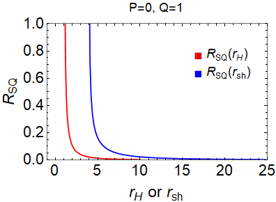
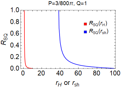
Fig. 1. Ruppeiner thermodynamic scalar curvature $R_{\rm SQ}$ with respect to the event horizon radius $r_{\rm H}$ and to the shadow radius $r_{\rm sh}$ at constant pressure $P$ and constant charge $Q$. Here we set $r_{\rm 0}=100$. The left graph corresponds to the RN black hole and the right one to the RN AdS black hole.

4 Relationship between shadow and thermodynamics in the aspects of phase transition and microstructure for Kerr (AdS) black holes

4.1 Hawking temperature and Ruppeiner thermodynamic scalar curvature with respect to event horizon radius

We take the Kerr (AdS) black hole as a representative of rotating black holes and study its relationship between shadow and thermodynamics in the aspects of phase transition and microstructure.

The line element of the Kerr AdS black hole takes [98] the form,

$$ds^{2} = -\frac{(\Delta_{r}-\Delta_{\theta}a^{2}\sin^{2}\theta)}{\Sigma}dt^{2}-\frac{2a\sin^{2}\theta}{\Xi\Sigma}[(r^{2}+a^{2})\Delta_{\theta}-\Delta_{r}]dtd\varphi+\frac{\Sigma}{\Delta_{r}}dr^{2}+\frac{\Sigma}{\Delta_{\theta}}d\theta^{2}$$ (38)

$$+\frac{\sin^{2}\theta}{\Xi^{2}\Sigma}[(r^{2}+a^{2})^{2}\Delta_{\theta}-\Delta_{r}a^{2}\sin^{2}\theta]d\varphi^{2},$$

with

$$\Sigma = r^{2}+a^{2}\cos^{2}\theta,$$ (39)

$$\Delta_{r} = \left(a^{2}+r^{2}\right)\left(1-\frac{\Lambda r^{2}}{3}\right)-2mr,$$ (40)

$$\Delta_{\theta} = 1+\frac{\Lambda}{3}a^{2}\cos^{2}\theta,$$ (41)

$$\Xi = 1+\frac{\Lambda}{3}a^{2},$$ (42)

where $m$ and $a$ are parameters related to the mass and rotation of the black hole, respectively. In the extended phase space including the cosmological constant $\Lambda$, some thermodynamic quantities for the Kerr AdS black hole read [58, 60, 61, 62, 63, 64] as follows:

$$M = H=\sqrt{\frac{(8PS+3)\left[12\pi^{2}J^{2}+S^{2}(8PS+3)\right]}{36\pi S}},$$ (43)

$$T = \frac{S^{2}\left(64P^{2}S^{2}+32PS+3\right)-12\pi^{2}J^{2}}{4\sqrt{S^{3}(8PS+3)\left[12\pi^{3}J^{2}+\pi S^{2}(8PS+3)\right]}},$$ (44)

$$\Omega = \frac{2\pi^{3/2}J\sqrt{8PS+3}}{\sqrt{S\left[12\pi^{2}J^{2}+S^{2}(8PS+3)\right]}},$$ (45)

$$V = \frac{4\sqrt{S}\left[6\pi^{2}J^{2}+S^{2}(8PS+3)\right]}{3\sqrt{8PS+3}\sqrt{12\pi^{3}J^{2}+\pi S^{2}(8PS+3)}},$$ (46)

$$S = \frac{\pi\left(a^{2}+r_{\rm H}^{2}\right)}{\Xi},$$ (47)

$$P = -\frac{\Lambda}{8\pi},$$ (48)

where the ADM mass $M=m/\Xi^{2}$ is regarded as the black hole enthalpy $H$, $T$ the Hawking temperature, $S$ the entropy, $V$ the thermo-volume, $J=Ma$ the angular momentum, $\Omega$ the angular velocity, $P$ the pressure, and $r_{\rm H}$ the event horizon radius. In addition, the first law of thermodynamics and the Smarr relation are [58, 60, 61, 62, 63, 64]

$$dM=TdS+VdP+\Omega dJ,$$ (49)

$$M=2(TS-PV+\Omega J).$$ (50)

The Ruppeiner line element describing this black hole in the phase space $\left\{S,J\right\}$ has [90] the form,

$$ds^{2}_{\rm R}=\frac{1}{T}\left(\frac{\partial T}{\partial S}\right)_{J}dS^{2}+\frac{2}{T}\left(\frac{\partial T}{\partial J}\right)_{S}dSdJ+\frac{1}{T}\left(\frac{\partial\Omega}{\partial J}\right)_{S}dJ^{2}.$$ (51)

Using Eqs. (44), (45), and (51), one can write [78, 90] the thermodynamic curvature,

$$R_{\rm SJ}=-\frac{1}{\sqrt{g}}\left[\frac{\partial}{\partial S}\left(\frac{g_{12}}{g_{11}\sqrt{g}}\frac{\partial g_{11}}{\partial J}-\frac{1}{\sqrt{g}}\frac{\partial g_{22}}{\partial S}\right)+\frac{\partial}{\partial J}\left(\frac{2}{\sqrt{g}}\frac{\partial g_{12}}{\partial S}-\frac{1}{\sqrt{g}}\frac{\partial g_{11}}{\partial J}-\frac{g_{12}}{g_{11}\sqrt{g}}\frac{\partial g_{11}}{\partial S}\right)\right],$$ (52)

where

$$g_{11} = -\frac{3S(4PS+1)}{12\pi^{2}J^{2}+S^{2}(8PS+3)}+\frac{2S\left[16PS(8PS+3)+3\right]}{S^{2}(8PS+1)(8PS+3)-12\pi^{2}J^{2}}-\frac{4P}{8PS+3}-\frac{3}{2S},$$ (53)

$$g_{12} = g_{21}=12\pi^{2}J\left[\frac{2}{12\pi^{2}J^{2}-S^{2}(8PS+1)(8PS+3)}-\frac{1}{12\pi^{2}J^{2}+S^{2}(8PS+3)}\right],$$ (54)

$$g_{22} = \frac{8\pi^{2}S^{5}(8PS+3)^{5/2}}{S^{2}\left[12\pi^{2}J^{2}+S^{2}(8PS+3)\right]\left[S^{2}(8PS+1)(8PS+3)-12\pi^{2}J^{2}\right]\sqrt{(8PS+3)}},$$ (55)

$$g = g_{11}g_{22}-g_{12}^{2}.$$ (56)

Substituting Eq. (47) into Eq. (44), and Eqs. (43) and (47) into Eq. (52), we know that the Hawking temperature $T$ and the Ruppeiner thermodynamic scalar curvature $R_{\rm SJ}$ are functions of $r_{\rm H}$, $J$, and $P$,

$$T = T(r_{\rm H},J,P),$$ (57)

$$R_{\rm SJ} = R_{\rm SJ}(r_{\rm H},J,P).$$ (58)

4.2 Hawking temperature and Ruppeiner thermodynamic scalar curvature with respect to shadow radius, or deformation parameters, or circularity deviation

The null geodesic equations of the photons around the Kerr AdS black hole can be expressed [40, 47] as

$$\frac{\mathrm{d}t}{\mathrm{d}\lambda} = \frac{\left(a^{2}\sin^{2}\theta+\Sigma\right)\left(a^{2}E\sin^{2}\theta-aL\Xi+\Sigma E\right)}{\Sigma\Delta_{r}}+\frac{a\left(L\Xi-aE\sin^{2}\theta\right)}{\Sigma\Delta_{\theta}},$$ (59)

$$\frac{\mathrm{d}r}{\mathrm{d}\lambda} = \frac{\sqrt{\left[E\left(a^{2}\sin^{2}\theta+\Sigma\right)-aL\Xi\right]^{2}-\Delta_{r}\left[(L\Xi-aE)^{2}+\text{K}\right]}}{\Sigma}\equiv\frac{\sqrt{U(r)}}{\Sigma},$$ (60)

$$\frac{\mathrm{d}\theta}{\mathrm{d}\lambda} = \frac{\sqrt{\Delta_{\theta}\left[(L\Xi-aE)^{2}+\text{K}\right]-(L\Xi\csc\theta-aE\sin\theta)^{2}}}{\Sigma}\equiv\frac{\sqrt{\Theta(\theta)}}{\Sigma},$$ (61)

$$\frac{\mathrm{d}\varphi}{\mathrm{d}\lambda} = \frac{a\Xi\left[E\left(a^{2}\sin^{2}\theta+\Sigma\right)-aL\Xi\right]}{\Sigma\Delta_{r}}+\frac{L\Xi^{2}-a\Xi E\sin^{2}\theta}{\Sigma\Delta_{\theta}\sin^{2}\theta},$$ (62)

where $L$ and $E$ are the angular momentum and energy of photons, respectively, $\lambda$ is the affine parameter, $K$ is the Carter constant, and $U(r)$ and $\Theta(\theta)$ are non-negative definite functions of $r$ and $\theta$, respectively.

The radius of the unstable orbit of photons $r_{\rm p}$ can be solved [40, 47] from the following conditions:

$$U(r_{\rm p})=0,\qquad\left.\frac{\mathrm{d}U(r)}{\mathrm{d}r}\right|_{r=r_{\rm p}}=0,$$ (63)

where the definition of $U(r)$ is given in Eq. (60). The two conditions can be expressed explicitly as [40, 47]

$$L_{E} \equiv \frac{L}{E}=\frac{3\left[a^{4}\Lambda r_{\rm p}+a^{2}\left(3m+\Lambda r_{\rm p}^{3}+3r_{\rm p}\right)+3r_{\rm p}^{2}\left(r_{\rm p}-3m\right)\right]}{a\left(a^{2}\Lambda+3\right)\left[r_{\rm p}\left(a^{2}\Lambda+2\Lambda r_{\rm p}^{2}-3\right)+3m\right]},$$ (64)

$$K_{E} \equiv \frac{K}{E^{2}}=-\frac{r_{\rm p}^{3}\left\{a^{4}\Lambda^{2}r_{\rm p}^{3}+6a^{2}\left[3m\left(\Lambda r_{\rm p}^{2}-2\right)+\Lambda r_{\rm p}^{3}\right]+9r_{\rm p}\left(r_{\rm p}-3m\right)^{2}\right\}}{a^{2}\left[r_{\rm p}\left(a^{2}\Lambda+2\Lambda r_{\rm p}^{2}-3\right)+3m\right]^{2}}.$$ (65)

After substituting Eqs. (64) and (65) into Eq. (61), one can determine the value range of $r_{\rm p}$,

$$r_{\rm p}\in[r_{\rm p1},r_{\rm p2}].$$ (66)

To describe the contour of the black hole shadow, we consider an observer located in the zero-angular-momentum reference frame [99] as follows:

$$\hat{e}_{(t)} = \sqrt{\frac{g_{\varphi\varphi}}{g_{t\varphi}^{2}-g_{tt}g_{\varphi\varphi}}}\left(\partial_{t}-\frac{g_{t\varphi}}{g_{\varphi\varphi}}\partial_{\varphi}\right),$$ (67)

$$\hat{e}_{(r)} = \frac{1}{\sqrt{g_{rr}}}\partial_{r},$$ (68)

$$\hat{e}_{(\theta)} = \frac{1}{\sqrt{g_{\theta\theta}}}\partial_{\theta},$$ (69)

$$\hat{e}_{(\varphi)} = \frac{1}{\sqrt{g_{\varphi\varphi}}}\partial_{\varphi},$$ (70)

where the timelike vector $\hat{e}_{(t)}$ and the spacelike vectors $\hat{e}_{(r)}$, $\hat{e}_{(\theta)}$, $\hat{e}_{(\varphi)}$ are normalized orthogonally to each other. For null geodesics, the four momentum $p^{\mu}$ of photons can be projected [47] onto the four bases of the observer’s frame, i.e.

$$p^{(t)} = -p_{\mu}\hat{e}^{\mu}_{(t)},$$ (71)

$$p^{(i)} = p_{\mu}\hat{e}^{\mu}_{(i)},$$ (72)

where the index $i$ means the space coordinates, $r,\theta,\varphi$.

The observation angles $(\alpha,\beta)$ are introduced [100] by the formulas,

$$p^{(r)} = p^{(t)}\cos\alpha\cos\beta,$$ (73)

$$p^{(\theta)} = p^{(t)}\sin\alpha,$$ (74)

$$p^{(\varphi)} = p^{(t)}\cos\alpha\sin\beta.$$ (75)

Combining Eqs. (59)-(75), one can obtain [73, 47] the relations satisfied by the observation angles,

$$\sin\alpha = \frac{p^{(\theta)}}{p^{(t)}}=\left.\pm\frac{1}{\hat{e}^{t}_{(t)}-L_{E}\hat{e}^{\varphi}_{(t)}}\sqrt{\frac{{\Delta_{\theta}\left[(L_{E}\Xi-a)^{2}+K_{E}\right]-(L_{E}\Xi\csc\theta-a\sin\theta)^{2}}}{\Sigma\Delta_{\theta}}}\right|_{(r_{0},\theta_{0})},$$ (76)

$$\tan\beta = \left.\frac{p^{(\varphi)}}{p^{(r)}}=L_{E}{\sqrt{\frac{\Sigma\Delta_{r}}{{g_{\varphi\varphi}\left[\left(a^{2}\sin^{2}\theta-aL_{E}\Xi+\Sigma\right)^{2}-\Delta_{r}\left((L_{E}\Xi-a)^{2}+K_{E}\right)\right]}}}}\right|_{(r_{0},\theta_{0})},$$ (77)

where $r_{0}$ is the distance between the observer and the black hole, and $\theta_{0}$ is the inclination angle between the observer’s sight line and the black hole’s rotation axis. In addition, one can determine the apparent position on the sky plane of the observer by introducing the following Cartesian coordinates [94, 46, 47],

$$x = -r_{0}\cos\alpha\sin\beta,$$ (78)

$$y = r_{0}\sin\alpha.$$ (79)

According to the schematic diagram in Fig. 2, the shadow radius $r_{\rm sh}$, the deformation parameters, $\delta_{s}$ and $k_{s}$, and the circularity deviation $\Delta C$ for a rotating black hole can be defined [101, 102, 103, 104] as follows:

$$r_{\rm sh} \equiv \frac{1}{2\pi}\int_{0}^{2\pi}l(\phi)d\phi,$$ (80)

$$\delta_{s} \equiv \frac{2r_{\rm sh}-(x_{\rm max}-x_{\rm min})}{r_{\rm sh}},$$ (81)

$$k_{s} \equiv \frac{2y_{h}}{x_{\rm max}-x_{\rm min}},$$ (82)

$$\Delta C \equiv 2\sqrt{\frac{1}{2\pi}\int_{0}^{2\pi}(l(\phi)-r_{\rm sh})^{2}d\phi},$$ (83)

where

$$l(\phi) \equiv \sqrt{(x-x_{c})^{2}+(y-y_{c})^{2}},$$ (84)

$$x_{c} \equiv \frac{|x_{\rm min}+x_{\rm max}|}{2},$$ (85)

$$y_{c} \equiv 0,$$ (86)

$$\tan\phi \equiv \frac{y-y_{c}}{x-x_{c}}.$$ (87)

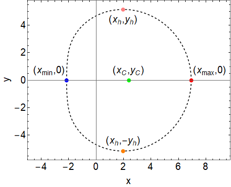
Figure 2. A schematic diagram for a rotating black hole shadow.

Since the Kerr AdS black hole is completely determined by only three parameters ($m$, $J$, $P$), we obtain the results,

$$r_{\rm sh} = r_{\rm sh}(r_{\rm H},J,P),$$ (88)

$$\delta_{s} = \delta_{s}(r_{\rm H},J,P),$$ (89)

$$k_{s} = k_{s}(r_{\rm H},J,P),$$ (90)

$$\Delta C = \Delta C(r_{\rm H},J,P).$$ (91)

This means that the shadow radius, deformation parameters, and circularity deviation can be expressed as functions of the event horizon radius, angular momentum, and pressure.

According to Eqs. (57) and (58) and Eqs. (88)-(91), we can express both the Hawking temperature $T$ and the Ruppeiner thermodynamic scalar curvature $R_{\rm SJ}$ as a one-variable function of the shadow radius $r_{\rm sh}$, or the deformation parameter $\delta_{s}$ or $k_{s}$, or the circularity deviation $\Delta C$ for the Kerr (AdS) black hole if the angular momentum $J$ and pressure $P$ are fixed,

$$T=\left.T(r_{\rm sh})\right|_{J,\,P},\qquad R_{\rm SJ}=\left.R_{\rm SJ}(r_{\rm sh})\right|_{J,\,P},$$ (92)

$$T=\left.T(\delta_{s})\right|_{J,\,P},\qquad R_{\rm SJ}=\left.R_{\rm SJ}(\delta_{s})\right|_{J,\,P},$$ (93)

$$T=\left.T(k_{s})\right|_{J,\,P},\qquad R_{\rm SJ}=\left.R_{\rm SJ}(k_{s})\right|_{J,\,P},$$ (94)

$$T=\left.T(\Delta C)\right|_{J,\,P},\qquad R_{\rm SJ}=\left.R_{\rm SJ}(\Delta C)\right|_{J,\,P}.$$ (95)

Based on Eqs. (88)-(91), we depict in Figs. 3 and 4 for the Kerr and Kerr AdS black holes, respectively, the relations of the shadow radius $r_{\rm sh}$, the deformation parameters $\delta_{s}$ and $k_{s}$, and the circularity deviation $\Delta C$ with respect to the horizon radius $r_{\rm H}$ for different inclination angles $\theta_{0}$ at constant pressure $P$ and angular momentum $J$. We can see that $r_{\rm sh}$ monotonically increases, but $\delta_{s}$, $k_{s}$ and $\Delta C$ monotonically decrease with increasing of $r_{\rm H}$, which means

$$\frac{\mathrm{d}r_{\rm sh}}{\mathrm{d}r_{\rm H}}>0,\qquad\frac{\mathrm{d}(1/\delta_{s})}{\mathrm{d}r_{\rm H}}>0,\qquad\frac{\mathrm{d}(1/k_{s})}{\mathrm{d}r_{\rm H}}>0,\qquad\frac{\mathrm{d}(1/\Delta C)}{\mathrm{d}r_{\rm H}}>0.$$ (96)

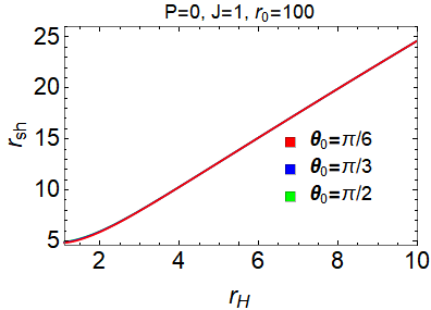
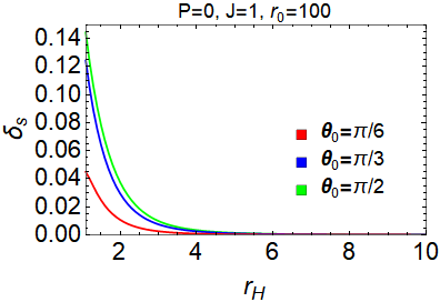
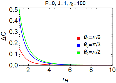
Fig. 3. The shadow radius $r_{\rm sh}$, the deformation parameters $\delta_{s}$ and $k_{s}$, and the circularity deviation $\Delta C$ with respect to the horizon radius $r_{\rm H}$ at constant pressure $P$ and angular momentum $J$ for the Kerr black hole.

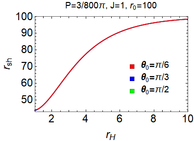
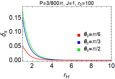
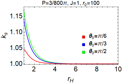
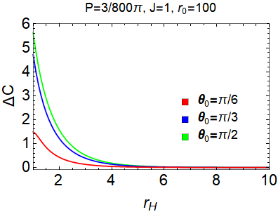
Fig. 4. The shadow radius $r_{\rm sh}$, the deformation parameters $\delta_{s}$ and $k_{s}$, and the circularity deviation $\Delta C$ with respect to the horizon radius $r_{\rm H}$ at constant pressure $P$ and angular momentum $J$ for the Kerr AdS black hole.

Considering $\frac{\partial T}{\partial r_{\rm H}}=\frac{\partial T}{\partial r_{\rm sh}}\frac{\mathrm{d}r_{\rm sh}}{\mathrm{d}r_{\rm H}}$, $\frac{\partial R_{\rm SJ}}{\partial r_{\rm H}}=\frac{\partial R_{\rm SJ}}{\partial r_{\rm sh}}\frac{\mathrm{d}r_{\rm sh}}{\mathrm{d}r_{\rm H}}$, and Eq. (96), we find that the positivity or negativity of $\frac{\partial T}{\partial r_{\rm H}}$ and $\frac{\partial R_{\rm SJ}}{\partial r_{\rm H}}$ depends entirely on the positivity or negativity of $\frac{\partial T}{\partial r_{\rm sh}}$ and $\frac{\partial R_{\rm SJ}}{\partial r_{\rm sh}}$, respectively. As a result, the conditions

$$\frac{\partial T}{\partial r_{\rm H}}>0,\qquad\frac{\partial T}{\partial r_{\rm H}}=0,\qquad\frac{\partial T}{\partial r_{\rm H}}<0,$$ (97)

and

$$\frac{\partial R_{\rm SJ}}{\partial r_{\rm H}}>0,\qquad\frac{\partial R_{\rm SJ}}{\partial r_{\rm H}}=0,\qquad\frac{\partial R_{\rm SJ}}{\partial r_{\rm H}}<0,$$ (98)

can be converted to

$$\frac{\partial T}{\partial r_{\rm sh}}>0,\qquad\frac{\partial T}{\partial r_{\rm sh}}=0,\qquad\frac{\partial T}{\partial r_{\rm sh}}<0,$$ (99)

$$\frac{\partial T}{\partial(1/\delta_{s})}>0,\qquad\frac{\partial T}{\partial(1/\delta_{s})}=0,\qquad\frac{\partial T}{\partial(1/\delta_{s})}<0,$$ (100)

$$\frac{\partial T}{\partial(1/k_{s})}>0,\qquad\frac{\partial T}{\partial(1/k_{s})}=0,\qquad\frac{\partial T}{\partial(1/k_{s})}<0,$$ (101)

$$\frac{\partial T}{\partial(1/\Delta C)}>0,\qquad\frac{\partial T}{\partial(1/\Delta C)}=0,\qquad\frac{\partial T}{\partial(1/\Delta C)}<0,$$ (102)

and

$$\frac{\partial R_{\rm SJ}}{\partial r_{\rm sh}}>0,\qquad\frac{\partial R_{\rm SJ}}{\partial r_{\rm sh}}=0,\qquad\frac{\partial R_{\rm SJ}}{\partial r_{\rm sh}}<0,$$ (103)

$$\frac{\partial R_{\rm SJ}}{\partial(1/\delta_{s})}>0,\qquad\frac{\partial R_{\rm SJ}}{\partial(1/\delta_{s})}=0,\qquad\frac{\partial R_{\rm SJ}}{\partial(1/\delta_{s})}<0,$$ (104)

$$\frac{\partial R_{\rm SJ}}{\partial(1/k_{s})}>0,\qquad\frac{\partial R_{\rm SJ}}{\partial(1/k_{s})}=0,\qquad\frac{\partial R_{\rm SJ}}{\partial(1/k_{s})}<0,$$ (105)

$$\frac{\partial R_{\rm SJ}}{\partial(1/\Delta C)}>0,\qquad\frac{\partial R_{\rm SJ}}{\partial(1/\Delta C)}=0,\qquad\frac{\partial R_{\rm SJ}}{\partial(1/\Delta C)}<0.$$ (106)

In order to test whether the relations Eqs. (97)-(106) are valid or not, according to Eqs. (92)-(95) we draw the Hawking temperature $T$ and the Ruppeiner thermodynamic scalar curvature $R_{\rm SJ}$ of the Kerr (AdS) black hole as a function of $r_{\rm sh}$, or $1/\delta_{s}$, or $1/k_{s}$, or $1/\Delta C$, respectively, at constant pressure $P$ and angular momentum $J$ in Figs. 5-8, where the red curves $T-r_{\rm H}$ (Eq. (57)) and $R_{\rm SJ}-r_{\rm H}$ (Eq. (58)) are attached as a comparison.

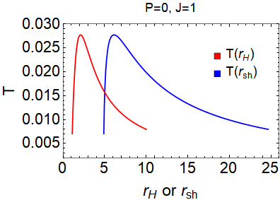
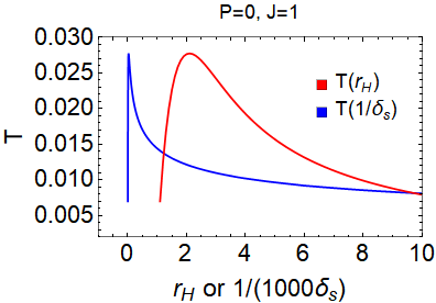
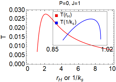
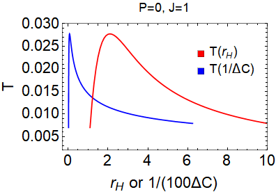
Fig. 5. The Hawking temperature $T$ of the Kerr black hole as a function of $r_{\rm sh}$, or $1/\delta_{s}$, or $1/k_{s}$, or $1/\Delta C$ at constant pressure $P$ and angular momentum $J$, where the red curves of the Hawking temperature $T$ of the Kerr black hole as a function of $r_{\rm H}$ are attached for comparison. Here we set $r_{\rm 0}=100$ and $\theta_{\rm 0}=\frac{\pi}{2}$.

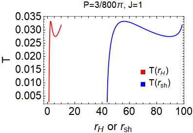
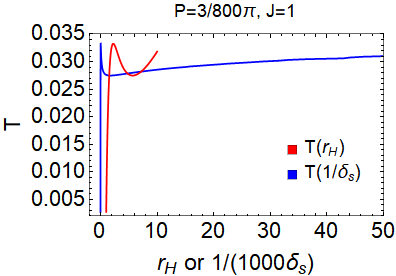
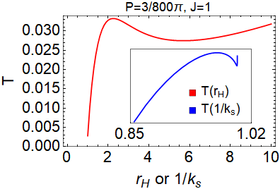
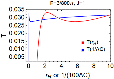
Fig. 6. The Hawking temperature $T$ of the Kerr AdS black hole as a function of $r_{\rm sh}$, or $1/\delta_{s}$, or $1/k_{s}$, or $1/\Delta C$ at constant pressure $P$ and angular momentum $J$, where the red curves of the Hawking temperature $T$ of the Kerr AdS black hole as a function of $r_{\rm H}$ are attached for comparison. Here we set $r_{\rm 0}=100$ and $\theta_{\rm 0}=\frac{\pi}{2}$.

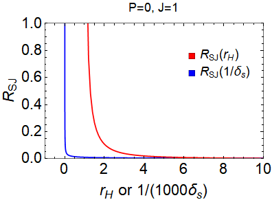
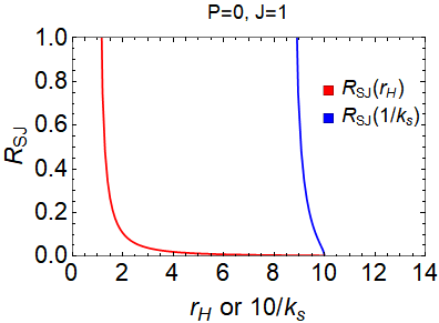
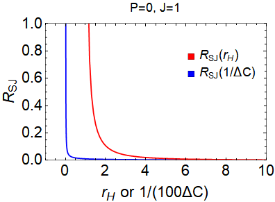
Fig. 7. The Ruppeiner thermodynamic scalar curvature $R_{\rm SJ}$ of the Kerr black hole as a function of $r_{\rm sh}$, or $1/\delta_{s}$, or $1/k_{s}$, or $1/\Delta C$ at constant pressure $P$ and angular momentum $J$, where the red curves of the Ruppeiner curvature $R_{\rm SJ}$ of the Kerr black hole as a function of $r_{\rm H}$ are attached for comparison. Here we set $r_{\rm 0}=100$ and $\theta_{\rm 0}=\frac{\pi}{2}$.

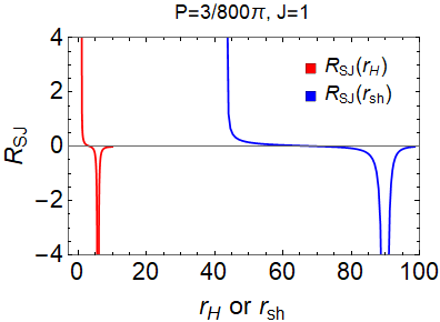
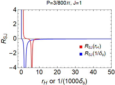
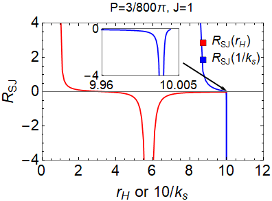
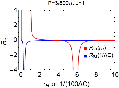
Fig. 8. The Ruppeiner thermodynamic scalar curvature $R_{\rm SJ}$ of the Kerr AdS black hole as a function of $r_{\rm sh}$, or $1/\delta_{s}$, or $1/k_{s}$, or $1/\Delta C$ at constant pressure $P$ and angular momentum $J$, where the red curves of the Ruppeiner curvature $R_{\rm SJ}$ of the Kerr AdS black hole as a function of $r_{\rm H}$ are attached for comparison. Here we set $r_{\rm 0}=100$ and $\theta_{\rm 0}=\frac{\pi}{2}$.

By comparing the blue curves and red curves in Figs. 5 and 6, we can clearly see that the blue curves $T-r_{\rm sh}$, $T-1/\delta_{s}$, $T-1/k_{s}$, and $T-1/\Delta C$ have similar profiles with the red curve $T-r_{\rm H}$, which indicates that the shadow radius $r_{\rm sh}$, the deformation parameters $\delta_{s}$ and $k_{s}$, and the circularity deviation $\Delta C$ can connect to the phase transition of black holes. Moreover, we can see clearly in Figs. 7 and 8 that the blue curves $R_{\rm SJ}-r_{\rm sh}$, $R_{\rm SJ}-1/\delta_{s}$, $R_{\rm SJ}-1/k_{s}$, and $R_{\rm SJ}-1/\Delta C$ have similar profiles with the red curve $R_{\rm SJ}-r_{\rm H}$, which indicates that the shadow radius $r_{\rm sh}$, the deformation parameters $\delta_{s}$ and $k_{s}$, and the circularity deviation $\Delta C$ can connect to the black hole microstructure. Here we note that our choice of shadow deformation parameters comes from Refs. [102, 103] but not from Ref. [73] because the former is able to reflect the thermodynamics of the Kerr (AdS) black hole, while the latter is not.

Finally, we point out that the equivalence between Eqs. (57)-(58) and Eqs. (97)-(106) is also valid for the Kerr dS black hole with negative pressure. We verify this result by depicting the relations of $r_{\rm sh}$, $\delta_{s}$, $k_{s}$, and $\Delta C$ with respect to $r_{\rm H}$ at different inclination angles $\theta_{0}$ but at fixed pressure $P$ and angular momentum $J$ in Fig. 9. We can see that $r_{\rm sh}$ monotonically increases but $\delta_{s}$, $k_{s}$, and $\Delta C$ monotonically decrease with increasing of $r_{\rm H}$, which is similar to the situation in Fig. 4. As a result, we conclude that the four observables, $r_{\rm sh}$, $\delta_{s}$, $k_{s}$, and $\Delta C$, describing the characteristics of shadows are good enough to have a close connection to the thermodynamics of Kerr (A)dS black holes.

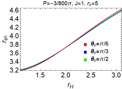
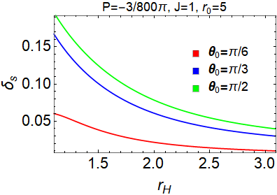
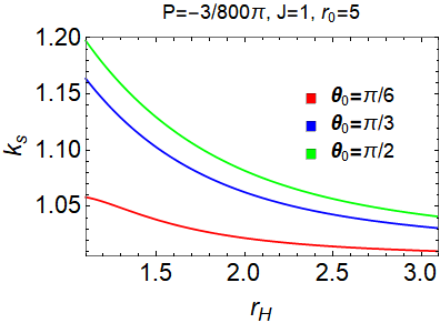
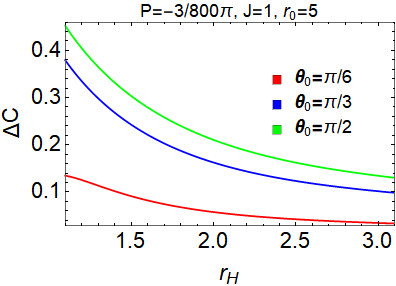
Fig. 9. The shadow radius $r_{\rm sh}$, the deformation parameters $\delta_{s}$ and $k_{s}$, and the circularity deviation $\Delta C$ with respect to the horizon radius $r_{\rm H}$ at constant pressure $P$ and angular momentum $J$ for the Kerr dS black hole.

5 Constraint to the relaxation time of black hole perturbation based on shadow data

In this section, we use the shadow data to impose a constraint on the relaxation time defined as the period that a perturbed black hole returns to its stable configuration. Based on the principle of causality and the second law of thermodynamics, Bekenstein proposed [105, 106] the universal bound on the information emission rate of a physical system. Later, in terms of the laws of black hole thermodynamics, Hod developed Bekenstein’s idea and derived [107, 108] a universal bound on the relaxation time of a perturbed thermodynamic system, which is known as the Bekenstein-Hod universal bound,

$$\tau\geq\frac{\hbar}{\pi k_{\rm B}T},$$ (107)

where $\tau$ represents the relaxation time and can be regarded [107, 108] as $1/|\omega_{\rm I}|$, and $|\omega_{\rm I}|$ denotes the absolute value of imaginary part of fundamental and least damped quasinormal resonances. Moreover, the Bekenstein-Hod universal bound is also related to [109, 110, 111] the viscosity-entropy bound. Based on the remnant of binary black hole merger observed by LIGO and Virgo [112, 113], this bound has recently been tested [114] by the astrophysical black hole population with $94\%$ probability.

According to the latest shadow data [1, 48, 49, 50] of the M$87^{*}$ black hole, the angular size of the shadow is $\delta=(42\pm 3)$ $\mu as$ (microarcsecond), the distance to the black hole $D=16.8_{-0.8}^{+0.8}$ Mpc (million parsec), and the black hole mass $M=(6.5\pm 0.7)\times 10^{9}M_{\bigodot}$. As a consequence, the shadow diameter $d_{{\rm M}87^{*}}$ in terms of the unit of mass is [48, 49]

$$d_{{\rm M}87^{*}}\equiv\frac{D\delta}{M}\approx 11.0\pm 1.5,$$ (108)

which means that the range of the shadow diameter is $9.5\lesssim d_{{\rm M}87^{*}}=2r_{\rm sh}\lesssim 12.5$ in the $1\sigma$ confidence region. In addition, the range of the circularity deviation $\Delta C$ of the M$87^{*}$ shadow reads [1]: $\Delta C\leqslant 0.1$. If the M$87^{*}$ black hole is regarded as the Reissner-Nordström (RN) black hole, i.e., matching the shadow data to the RN black hole, we have the available ranges of charge $Q$ and Hawking temperature $T$; if the M$87^{*}$ black hole is regarded as the Kerr black hole, i.e., matching the shadow data to suit the Kerr black hole, we have the available ranges of angular momentum $J$ and Hawking temperature $T$. These ranges are shown in the left and right diagrams of Fig. 10, respectively.

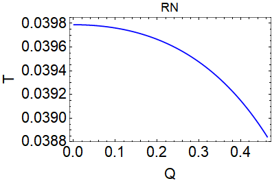
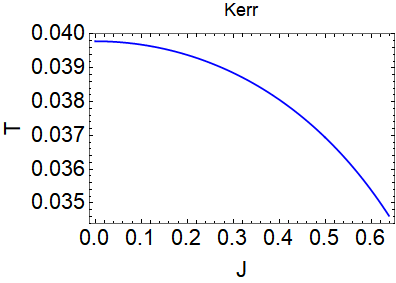
Fig. 10. The Hawking temperature $T$ with respect to the charge $Q$ in the left diagram if matching the shadow data of the M$87^{*}$ black hole to suit the RN black hole, and the Hawking temperature $T$ with respect to the angular momentum $J$ in the right diagram if matching the shadow data of the M$87^{*}$ black hole to suit the Kerr black hole. Here we set $M=1$.

Combining Fig. 10 with Eq. (107), we can deduce the value range of the relaxation time $\tau$ for the RN black hole and the Kerr black hole, respectively, when matching the shadow data of the M$87^{*}$ black hole to suit them,

$$\tau^{\rm RN}\geq\tau_{\rm min}^{\rm RN},\qquad\tau_{\rm min}^{\rm RN}\in[8,8.2],$$ (109)

$$\tau^{\rm Kerr}\geq\tau_{\rm min}^{\rm Kerr},\qquad\tau_{\rm min}^{\rm Kerr}\in[8,9.2].$$ (110)

From Fig. 10 we can see that the increase of charge $Q$ ($Q\equiv q^{2}$) and angular momentum $J$ will make the Hawking temperature $T$ decrease when the black hole mass $M$ is fixed, which is shown by the blue curves. This implies that the Schwarzschild black hole has the largest Hawking temperature $T_{\rm max}=\frac{\hbar c^{3}}{8\pi k_{\rm B}GM}$ at a fixed black hole mass. Therefore, by substituting the largest Hawking temperature $T_{\rm max}$ into Eq. (107), one can obtain [111] the minimum relaxation time at a fixed black hole mass $M$,

$$\tau_{\rm min}=\frac{8GM}{c^{3}}.$$ (111)

Using Eq. (111), we know that the relaxation time for the perturbed M$87^{*}$ black hole to return to its equilibrium equals at least,

$$\tau_{\rm min}^{{\rm M}87^{*}}=\frac{8GM_{{\rm M}87^{*}}}{c^{3}}=256149\;{\rm seconds}\approx 3\;{\rm days},$$ (112)

where $M_{{\rm M}87^{*}}=6.5\times 10^{9}M_{\bigodot}$. Similarly, we obtain the corresponding minimum relaxation time of the Sgr $A^{*}$ black hole,

$$\tau_{\rm min}^{{\rm Sgr}\,A^{*}}=\frac{8GM_{{\rm Sgr}\,A^{*}}}{c^{3}}=158.42\;{\rm seconds}\approx 2.64\;{\rm minutes},$$ (113)

where the mass of the supermassive black hole in the center of the Milky Way is [115]: $M_{{\rm Sgr}\,A^{*}}=4.02\times 10^{6}M_{\bigodot}$.

In addition, we can know that the Schwarzschild black hole has [39, 116] the largest shadow size at a fixed black hole mass $M$,

$$r_{\rm sh}^{\rm max}=\frac{3\sqrt{3}GM}{c^{2}}.$$ (114)

Using Eqs. (111) and (114), we obtain the linear relationship between the minimum relaxation time $\tau_{\rm min}$ and the maximum shadow radius $r_{\rm sh}^{\rm max}$,

$$\tau_{\rm min}=\frac{8\sqrt{3}}{9c}r_{\rm sh}^{\rm max},$$ (115)

and for the first time plot the graph of the minimum relaxation time $\tau_{\rm min}$ with respect to the maximum shadow radius $r_{\rm sh}^{\rm max}$ for different black hole mass levels in Fig. 11.

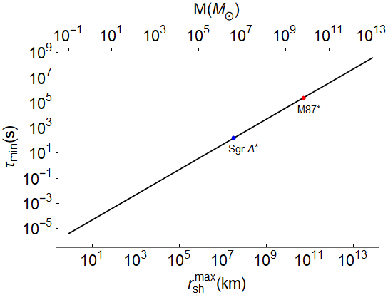
Fig. 11. The minimum relaxation time $\tau_{\rm min}$ with respect to the maximum shadow radius $r_{\rm sh}^{\rm max}$ for different black hole mass levels. The coordinates of the red dot are (6.5$\times$$10^{9}$, 4.98775$\times$$10^{10}$, 256149), which represents the mass, the maximum shadow radius, and the minimum relaxation time of the M$87^{*}$ black hole, while the coordinates of the blue dot are (4.02$\times$$10^{6}$, 3.08473$\times$$10^{7}$, 158.42), which represents the mass, the maximum shadow radius, and the minimum relaxation time of the Sgr $A^{*}$ black hole.

We note that Eq. (115) has a certain universality for asymptotically flat black holes, but not for asymptotically non-flat black holes. From Fig. 11, we draw the following conclusions:

• When the black hole mass $M$ is fixed, there exists a linear relationship between the minimum relaxation time $\tau_{\rm min}$ and the maximum shadow radius $r_{\rm sh}^{\rm max}$, where the former represents the thermodynamics of black holes while the latter the dynamics of black holes. Quite interesting is that the thermodynamic effect is proportional to the dynamic one.

• Given the mass $M$ of a celestial black hole, we can know the minimum relaxation time $\tau_{\rm min}$ and the maximum shadow radius $r_{\rm sh}^{\rm max}$ in terms of this figure. For example, using the mass of the M$87^{*}$ black hole and the mass of the Sgr $A^{*}$ black hole, we can mark the minimum relaxation time and the maximum shadow radius of the two black holes in this figure. The two points are located on a line. Using this line, we can predict the minimum relaxation time and the maximum shadow radius for a new black hole when its mass is measured.

We look forward to verifying Fig. 11 by using more shadow data and gravitational wave data of celestial black holes from astronomical observations in the future.

6 Conclusion

In this paper, at first we investigate the relationship between the shadow radius and microstructure for a general static spherically symmetric black hole, and then turn to the relationship between the shadow and thermodynamics in the aspects of phase transition and microstructure for the Kerr (AdS) black hole. Moreover, we give the constraint to the relaxation time of black hole perturbation by combining the shadow data with the Bekenstein-Hod universal bound. We summarize our main results as follows.

• The shadow radius of a general static spherically symmetric black hole can reflect the black hole microstructure.

• The four observables, the shadow radius $r_{\rm sh}$, the deformation parameters $\delta_{s}$ and $k_{s}$, and the circularity deviation $\Delta C$, describing the shadow characteristics of the Kerr (A)dS black hole can reflect the black hole thermodynamics in the aspects of phase transition and microstructure.

• We predict that the minimum relaxation times of M$87^{*}$ black hole and Sgr $A^{*}$ black hole are approximately 3 days and 2.64 minutes, respectively. Moreover, we plot Fig. 11 describing the relation among the three parameters, $(M,r_{\rm sh}^{\rm max},\tau_{\rm min})$, on a plane, and expect it to be verified in the future.

In a word, there exists a close relationship between dynamics and thermodynamics of black holes, where the black hole shadow represents dynamics, the Hawking temperature $T$ describes phase transitions, and the thermodynamic curvature scalar $R$ reflects black hole microstructure. This shows that the unobservable black hole thermodynamics can indeed be revealed by the observable dynamics. Especially, the shadow is a good enough observable to unfold the black hole thermodynamics.

References

- [1] EHT Collaboration, First M87 event horizon telescope results. I. The shadow of the supermassive black hole, Astrophys. J. 875 (2019) L1 [arXiv:1906.11238 [astro-ph.GA]].
- [2] EHT Collaboration, First M87 event horizon telescope results. IV. Imaging the central supermassive black hole, Astrophys. J. 875 (2019) L4 [arXiv:1906.11241 [astro-ph.GA]].
- [3] A.F. Zakharov, F. de Paolis, G. Ingrosso, and A.A. Nucita, Shadows as a tool to evaluate black hole parameters and a dimension of spacetime, New Astron. Rev. 56 (2012) 64.
- [4] N. Tsukamoto, Z. Li, and C. Bambi, Constraining the spin and the deformation parameters from the black hole shadow, JCAP 06 (2014) 043 [arXiv:1403.0371 [gr-qc]].
- [5] R. Kumar and S.G. Ghosh, Black hole parameter estimation from its shadow, APJ 892 (2020) 78 [arXiv:1811.01260 [gr-qc]].
- [6] M. Khodadi, A. Allahyari, S. Vagnozzi, and D.F. Mota, Black holes with scalar hair in light of the Event Horizon Telescope, JCAP 09 (2020) 026 [arXiv:2005.05992 [gr-qc]].
- [7] P. Kocherlakota, et al., Constraints on black-hole charges with the 2017 EHT observations of M87, Phys. Rev. D 103 (2021) 104047 [arXiv:2105.09343 [gr-qc]].
- [8] Z.-Y. Xu, X. Hou, and J.-C. Wang, Possibility of identifying matter around rotating black hole with black hole shadow, JCAP 10 (2018) 046 [arXiv:1806.09415 [gr-qc]].
- [9] X. Hou, Z.-Y. Xu, and J.-C. Wang, Rotating black hole shadow in perfect fluid dark matter, JCAP 12 (2018)040 [arXiv:1810.06381 [gr-qc]].
- [10] K. Saurabh and K. Jusufi, Imprints of dark matter on black hole shadows using spherical accretions, Eur. Phys. J. C 81 (2021) 490 [arXiv:2009.10599 [gr-qc]].
- [11] R.A. Konoplya, Shadow of a black hole surrounded by dark matter, Phys. Lett. B 795 (2019) 1 [arXiv:1905.00064 [gr-qc]].
- [12] J.L. Synge, The escape of photons from gravitationally intense stars, Mon. Not. Roy. Astron. Soc. 131 (1966) 463.
- [13] J.P. Luminet, Image of a spherical black hole with thin accretion disk, Astron. Astrophys. 75 (1979) 228.
- [14] J.M. Bardeen, Timelike and null geodesics in the Kerr metric, in Black holes, edited by C. DeWitt and B. S. DeWitt (Gordon and Breach, New York, 1973), p. 215.
- [15] A. De Vries, The apparent shape of a rotating charged black hole, closed photon orbits and the bifurcation set A4, Class. Quantum Grav. 17 (2000) 123.
- [16] K. Hioki and U. Miyamoto, Hidden symmetries, null geodesics, and photon capture in the Sen black hole, Phys. Rev. D 78 (2008) 044007 [arXiv:0805.3146 [gr-qc]].
- [17] C. Bambi and K. Freese, Apparent shape of super-spinning black holes, Phys. Rev. D 79 (2009) 043002 [arXiv:0812.1328 [astro-ph]].
- [18] M. Guo, N.A. Obers, and H. Yan, Observational signatures of near-extremal Kerr-like black holes in a modified gravity theory at the Event Horizon Telescope, Phys. Rev. D 98 (2018) 084063 [arXiv:1806.05249 [gr-qc]].
- [19] R.A. Hennigar, M.B.J. Poshteh, and R.B. Mann, Shadows, signals, and stability in Einsteinian cubic gravity, Phys. Rev. D 97 (2018) 064041 [arXiv:1801.03223 [gr-qc]].
- [20] G.S. Bisnovatyi-Kogan and O.Y. Tsupko, Shadow of a black hole at cosmological distances, Phys. Rev. D 98 (2018) 084020 [arXiv:1805.03311 [gr-qc]].
- [21] V. Perlick, O.Y. Tsupko, and G.S. Bisnovatyi-Kogan, Black hole shadow in an expanding universe with a cosmological constant, Phys. Rev. D 97 (2018) 104062 [arXiv:1804.04898 [gr-qc]].
- [22] V. Perlick, O.Y. Tsupko, and G.S. Bisnovatyi-Kogan, Influence of a plasma on the shadow of a spherically symmetric black hole, Phys. Rev. D 92 (2015) 104031 [arXiv:1507.04217 [gr-qc]].
- [23] S.-W. Wei, Y.-C. Zou, Y.-X. Liu, and R.B. Mann, Curvature radius and Kerr black hole shadow, JCAP 08 (2019) 030 [arXiv:1904.07710 [gr-qc]].
- [24] R. Shaikh, Black hole shadow in a general rotating spacetime obtained through Newman-Janis algorithm, Phys. Rev. D 100 (2019) 024028 [arXiv:1904.08322 [gr-qc]].
- [25] S. Vagnozzi and L. Visinelli, Hunting for extra dimensions in the shadow of M87, Phys. Rev. D 100 (2019) 024020 [arXiv:1905.12421 [gr-qc]].
- [26] R.A. Konoplya, T. Pappas, and A. Zhidenko, Einstein-scalar-Gauss-Bonnet black holes: Analytical approximation for the metric and applications to calculations of shadows, Phys. Rev. D 101 (2020) 044054 [arXiv:1907.10112 [gr-qc]].
- [27] K. Jusufi, M. Jamil, and T. Zhu, Shadows of Sgr black hole surrounded by superfluid dark matter halo, Eur. Phys. J. C 80 (2020) 354 [arXiv:2005.05299 [gr-qc]].
- [28] J.W. Moffat, Modified gravity black holes and their observable shadows, Eur. Phys. J. C 75 (2015) 130 [arXiv:1502.01677 [gr-qc]].
- [29] J.W. Moffat and V.T. Toth, Masses and shadows of the black holes Sagittarius and in modified gravity, Phys. Rev. D 101 (2020) 024014.
- [30] M. Wang, S. Chen, J. Wang, and J. Jing, Shadow of a Schwarzschild black hole surrounded by a Bach-Weyl ring, Eur. Phys. J. C 80 (2020) 110 [arXiv:1904.12423 [gr-qc]].
- [31] A. Das, A. Saha, and S. Gangopadhyay, Shadow of charged black holes in Gauss-Bonnet gravity, Eur. Phys. J. C 80 (2020) 1 [arXiv:1909.01988 [gr-qc]].
- [32] C. Liu, T. Zhu, Q. Wu, et al., Shadow and quasinormal modes of a rotating loop quantum black hole, Phys. Rev. D 101 (2020) 084001 [arXiv:2003.00477 [gr-qc]].
- [33] I. Banerjee, S. Chakraborty, and S. SenGupta, Silhouette of M8: A new window to peek into the world of hidden dimensions, Phys. Rev. D 101 (2020) 041301 [arXiv:1909.09385 [gr-qc]].
- [34] X.-X. Zeng and H.-Q. Zhang, Influence of quintessence dark energy on the shadow of black hole, Eur. Phys. J. C 80 (2020) 1058 [arXiv:2007.06333 [gr-qc]].
- [35] A. Abdujabbarov, M. Amir, B. Ahmedov, and S.G. Ghosh, Shadow of rotating regular black holes, Phys. Rev. D 93 (2016) 104004 [arXiv:1604.03809 [gr-qc]].
- [36] R. Kumar, S.G. Ghosh, and A.-Z. Wang, Shadow cast and deflection of light by charged rotating regular black holes, Phys. Rev. D 100 (2019) 124024 [arXiv:1912.05154 [gr-qc]].
- [37] N. Tsukamoto, Black hole shadow in an asymptotically flat, stationary, and axisymmetric spacetime: The Kerr-Newman and rotating regular black holes, Phys. Rev. D 97 (2018) 064021 [arXiv:1708.07427 [gr-qc]].
- [38] R.A. Konoplya and A. Zhidenko, Analytical representation for metrics of scalarized Einstein-Maxwell black holes and their shadows, Phys. Rev. D 100 (2019) 044015 [arXiv:1907.05551 [gr-qc]].
- [39] H. Lu and H.-D. Lyu, Schwarzschild black holes have the largest size, Phys. Rev. D 101 (2020) 044059 [arXiv:1911.02019 [gr-qc]].
- [40] A. Grenzebach, V. Perlick, and C. Lämmerzahl, Photon regions and shadows of Kerr-Newman-NUT black holes with a cosmological constant, Phys. Rev. D 89 (2014) 124004 [arXiv:1403.5234 [gr-qc]].
- [41] J.C.S. Neves, Constraining the tidal charge of brane black holes using their shadows, Eur. Phys. J. C 80 (2020) 717 [arXiv:2005.00483 [gr-qc]].
- [42] J.C.S. Neves, Upper bound on the GUP parameter using the black hole shadow, Eur. Phys. J. C 80 (2020) 343 [arXiv:1906.11735 [gr-qc]].
- [43] E.F. Eiroa and C.M. Sendra, Shadow cast by rotating braneworld black holes with a cosmological constant, Eur. Phys. J. C 78 (2018) 91 [arXiv:1711.08380 [gr-qc]].
- [44] S. Haroon, M. Jamil, K. Jusufi, K. Lin, and R.B. Mann, Shadow and deflection angle of rotating black holes in perfect fluid dark matter with a cosmological constant, Phys. Rev. D 99 (2019) 044015 [arXiv:1810.04103 [gr-qc]].
- [45] R. Kumar, B.P. Singh, and S.G. Ghosh, Shadow and deflection angle of rotating black hole in asymptotically safe gravity, Ann. Phys. 420 (2020) 168252 [ arXiv:1904.07652 [gr-qc]].
- [46] M. Zhang and J. Jiang, NUT charges and black hole shadows, Phys. Lett. B 816 (2021) 136213 [arXiv:2103.11416 [gr-qc]].
- [47] P.-C. Li, M.-Y. Guo, and B. Chen, Shadow of a spinning black hole in an expanding universe, Phys. Rev. D 101 (2020) 084041 [arXiv:2001.04231 [gr-qc]].
- [48] C.Bambi, K. Freese, S. Vagnozzi and L. Visinelli, Testing the rotational nature of the supermassive object M8 from the circularity and size of its first image, Phys. Rev. D 100 (2019) 044057 [arXiv:1904.12983 [gr-qc]].
- [49] A. Allahyari, M. Khodadi, S. Vagnozzi, and D.F. Mota, Magnetically charged black holes from non-linear electrodynamics and the Event Horizon Telescope, JCAP 02 (2020) 003 [arXiv:1912.08231 [gr-qc]].
- [50] R. Kumar, A. Kumar, and S.G. Ghosh, Testing Rotating Regular Metrics as Candidates for Astrophysical Black Holes, Astrophys. J. 896 (2020) 89 [arXiv:2006.09869 [gr-qc]].
- [51] V. Perlick and O.Y. Tsupko, Calculating black hole shadows: review of analytical studies, [arXiv:2105.07101 [gr-qc]].
- [52] X.-C. Cai and Y.-G. Miao, Quasinormal modes and shadows of a new family of Ayón-Beato-García black holes, Phys. Rev. D 103 (2021) 124050 [arXiv:2104.09725 [gr-qc]].
- [53] X.-C. Cai and Y.-G. Miao, High-dimensional Schwarzschild black holes in scalar–tensor–vector gravity theory, Eur. Phys. J. C 81 (2021) 559 [arXiv: 2011.05542 [gr-qc]].
- [54] J.D. Bekenstein, Black holes and entropy, Phys. Rev. D 7 (1973) 2333.
- [55] J.M. Bardeen, B. Carter, and S.W. Hawking, The four laws of black hole mechanics, Commun. Math. Phys. 31 (1973) 161.
- [56] S.W. Hawking, Particle creation by black holes, Commun. Math. Phys. 43 (1975) 199.
- [57] D. Kubiznak, R. B. Mann, and M. Teo, Black hole chemistry: thermodynamics with Lambda, Class. Quant. Grav. 34 (2017) 063001 [arXiv:1608.06147 [hep-th]].
- [58] B.P. Dolan, Pressure and volume in the first law of black hole thermodynamics, Class. Quant. Grav. 28 (2011) 235017 [arXiv:1106.6260 [gr-qc]].
- [59] D. Kubiznak and R.B. Mann, criticality of charged AdS black holes, J. High Energy Phys. 07 (2012) 033 [arXiv:1205.0559 [hep-th]].
- [60] M.M. Caldarelli, G. Cognola, and D. Klemm, Thermodynamics of Kerr-Newman-AdS black holes and conformal field theories, Class. Quant. Grav. 17 (2000) 399 [arXiv: 9908022 [hep-th]].
- [61] P. Cheng, S.-W. Wei, and Y.-X. Liu, Critical phenomena in the extended phase space of Kerr-Newman-AdS black holes, Phys. Rev. D 94 (2016) 024025 [arXiv:1603.08694 [gr-qc]].
- [62] S.-W. Wei, P. Cheng, and Y.-X. Liu, Analytical and exact critical phenomena of d-dimensional singly spinning Kerr-AdS black holes, Phys. Rev. D 93 (2016) 084015 [arXiv:1510.00085 [gr-qc]].
- [63] N. Altamirano, D. Kubiznak, R.B. Mann, Z. Sherkatghanad, Thermodynamics of rotating black holes and black rings: phase transitions and thermodynamic volume, Galaxies 2 (2014) 89 [arXiv:1401.2586 [hep-th]].
- [64] N. Altamirano, D. Kubiznak, and R.B. Mann, Reentrant phase transitions in rotating anti-de Sitter black holes, Phys. Rev. D 88 (2013) 101502 [arXiv:1306.5756 [hep-th]].
- [65] S.-W. Wei and Y.-X. Liu, Photon orbits and thermodynamic phase transition of d-dimensional charged AdS black holes, Phys. Rev. D 97 (2018) 104027 [arXiv:1711.01522 [gr-qc]].
- [66] S.-W. Wei, Y.-X. Liu, and Y.-Q. Wang, Probing the relationship between the null geodesics and thermodynamic phase transition for rotating Kerr-AdS black holes, Phys. Rev. D 99 (2019) 044013 [arXiv:1807.03455 [gr-qc]].
- [67] B. Chandrasekhar and S. Mohapatra, A note on circular geodesics and phase transitions of black holes, Phys. Lett. B 791 (2019) 367 [arXiv:1805.05088 [hep-th]].
- [68] M. Zhang, S.-Z. Han, J. Jiang, and W.-B. Liu, Circular orbit of a test particle and phase transition of a black hole, Phys. Rev. D 99 (2019) 065016 [arXiv:1903.08293 [hep-th]].
- [69] Y.-M. Xu, H.-M. Wang, Y.-X. Liu, and S.-W. Wei, Photon sphere and reentrant phase transition of charged Born-Infeld-AdS black holes, Phys. Rev. D 100 (2019) 104044 [arXiv:1906.03334 [gr-qc]].
- [70] H. Li, Y. Chen, and S.J. Zhang, Photon orbits and phase transitions in Born-Infeld-dilaton black holes, Nucl. Phys. B 954 (2020) 114975 [arXiv:1908.09570 [hep-th]].
- [71] A.N. Kumara, C.L. Ahmed Rizwan, S. Punacha, et al., Photon orbits and thermodynamic phase transition of regular AdS black holes, Phys. Rev. D 102 (2020) 084059 [arXiv:1912.11909 [gr-qc]].
- [72] S.H. Hendi and Kh. Jafarzade, Critical behavior of charged AdS black holes surrounded by quintessence via an alternative phase space, Phys. Rev. D 103 (2021) 104011 [arXiv:2012.13271 [hep-th]].
- [73] M. Zhang and M.Guo, Can shadows reflect phase structures of black holes?, Eur. Phys. J. C 80 (2020) 790 [arXiv:1909.07033 [gr-qc]].
- [74] A. Belhaj, L. Chakhchi, H. El Moumni, J. Khalloufi, and K. Masmar, Thermal image and phase transitions of charged AdS black holes using shadow analysis, Int. J. Mod. Phys. A 35 (2020) 2050170 [arXiv:2005.05893 [gr-qc]].
- [75] G. Ruppeiner, Riemannian geometry in thermodynamic fluctuation theory, Rev. Mod. Phys. 67 (1995) 605; Erratum, Rev. Mod. Phys. 68 (1996) 313.
- [76] G. Ruppeiner, Thermodynamic curvature and phase transitions in Kerr-Newman black holes, Phys. Rev. D 78 (2008) 024016 [arXiv:0802.1326 [gr-qc]].
- [77] G. Ruppeiner, Thermodynamic curvature measures interactions, Am. J. Phys. 78 (2010) 1170 [arXiv:1007.2160 [cond-mat.stat-mech]].
- [78] G. Ruppeiner, Thermodynamic curvature and black holes, in Breaking of Supersymmetry and Ultraviolet Divergences in Extended Supergravity, edited by S. Bellucci, Springer Proceedings in Physics Vol. 153 (Springer, New York, 2014), p. 179 [arXiv:1309.0901 [gr-qc]].
- [79] R.-G. Cai and J. H. Cho, Thermodynamic curvature of the BTZ black hole, Phys. Rev. D 60 (1999) 067502 [arXiv:9803261[hep-th]].
- [80] J.-L. Zhang, R.-G. Cai, and H.-W. Yu, Phase transition and thermodynamical geometry for Schwarzschild AdS black hole in Ad spacetime, J. High Energy Phys. 02 (2015) 143 [arXiv:1409.5305 [hep-th]].
- [81] J.-L. Zhang, R.-G. Cai, and H.-W. Yu, Phase transition and thermodynamical geometry of Reissner-Nordström-AdS black holes in extended phase space, Phys. Rev. D 91 (2015) 044028 [arXiv:1502.01428 [hep-th]].
- [82] H.-S. Liu, H. Lu, M.-X Luo, and K.-N. Shao, Thermodynamical metrics and black hole phase transitions, J. High Energy Phys. 12 (2010) 054 [arXiv:1008.4482 [hep-th]].
- [83] K. Bhattacharya, S. Dey, B. R. Majhi, and S. Samanta, A general framework to study the extremal phase transition of black holes, Phys. Rev. D 99 (2019) 124047 [arXiv:1903.03434 [gr-qc]].
- [84] S.-W. Wei and Y.-X. Liu, Insight into the microscopic structure of an AdS black hole from a thermodynamical phase transition, Phys. Rev. Lett. 115 (2015) 111302 [arXiv:1502.00386 [gr-qc]].
- [85] Y.-G. Miao and Z.-M. Xu, Thermal molecular potential among micromolecules in charged AdS black holes, Phys. Rev. D 98 (2018) 044001 [arXiv:1712.00545 [hep-th]].
- [86] Y.-G. Miao and Z.-M. Xu, Interaction potential and thermocorrection to the equation of state for thermally stable Schwarzschild anti-de Sitter black holes, Sci. China-Phys. Mech. Astron. 62 (2019) 010412 [arXiv:1804.01743 [hep-th]].
- [87] S.-W. Wei, Y.-X. Liu, and R.B. Mann, Repulsive interactions and universal properties of charged anti-de Sitter black hole microstructures, Phys. Rev. Lett. 123 (2019) 071103 [arXiv:1906.10840 [gr-qc]].
- [88] S.-W. Wei, Y.-X. Liu, and R.B. Mann, Ruppeiner geometry, phase transitions, and the microstructure of charged AdS black holes, Phys. Rev. D 100 (2019) 124033 [arXiv:1909.03887 [gr-qc]].
- [89] S.-W. Wei and Y.-X. Liu, Intriguing microstructures of five-dimensional neutral Gauss-Bonnet AdS black hole, Phys. Lett. B 803 (2020) 135287 [arXiv:1910.04528 [gr-qc]].
- [90] R. Banerjee, S.K. Modak, and S. Samanta, Second order phase transition and thermodynamic geometry in Kerr-AdS black holes, Phys. Rev. D 84 (2011) 064024 [ arXiv:1005.4832 [hep-th]].
- [91] Z.-M. Xu, B. Wu, and W.-L. Yang, Fine micro-thermal structures for Reissner-Nordstrm black hole, Chin. Phys. C 44 (2020) 095106 [arXiv:1910.03378 [gr-qc]].
- [92] Z.-M. Xu, Analytic phase structures and thermodynamic curvature for the charged AdS black hole in alternative phase space, Front. Phys. 16 (2021) 24502 [arXiv:2011.06736 [gr-qc]].
- [93] B. Mirza and M. Zamaninasab, Ruppeiner geometry of RN black holes: flat or curved?, J. High Energy Phys. 06 (2007) 059 [arXiv:0706.3450 [hep-th]].
- [94] S. Chandrasekhar, The Mathematical Theory of Black Holes, Oxford University Press, Oxford, 1998.
- [95] Z.-M. Xu, B. Wu, and W.-L. Yang, Ruppeiner thermodynamic geometry for the Schwarzschild-AdS black hole, Phys. Rev. D 101 (2020) 024018 [arXiv:1910.12182 [gr-qc]].
- [96] A. Ghosh and C. Bhamidipati, Thermodynamic geometry for charged Gauss-Bonnet black holes in AdS spacetimes, Phys. Rev. D 101 (2020) 046005 [arXiv:1911.06280 [gr-qc]].
- [97] Z.-M. Xu, B. Wu, and W.-L. Yang, Thermodynamics curvature along the curves of Hawking-Page and first-order phase transitions, arXiv:2009.00291 [gr-qc].
- [98] B. Carter, Hamilton-Jacobi and Schrodinger separable solutions of Einstein’s equations, Commun. Math. Phys. 10 (1968) 280.
- [99] Z. Stuchlk, D. Charbulk, and J. Schee, Light escape cones in local reference frames of Kerrde Sitter black hole spacetimes and related black hole shadows, Eur. Phys. J. C 78 (2018) 180 [ arXiv:1811.00072 [gr-qc]].
- [100] P.V.P. Cunha, C.A.R. Herdeiro, E. Radu, and H.F. Runarsson, Shadows of Kerr black holes with and without scalar hair, Int. J. Mod. Phys. D 25 (2016) 1641021 [arXiv:1605.08293 [gr-qc]].
- [101] K. Hioki and K. Maeda, Measurement of the Kerr spin parameter by observation of a compact object’s shadow, Phys. Rev. D 80 (2009) 024042 [arXiv:0904.3575 [astro-ph.HE]].
- [102] T. Johannsen, Photon rings around Kerr and Kerr-like black holes, Astrophys. J. 777 (2013) 170 [arXiv:1501.02814 [astro-ph.HE]].
- [103] T. Johannsen and D. Psaltis, Testing the no-hair theorem with observations in the electromagnetic spectrum. II. Black hole images, Astrophys. J. 718 (2010) 446 [arXiv:1005.1931 [astro-ph.HE]].
- [104] O.Y. Tsupko, Analytical calculation of black hole spin using deformation of the shadow, Phys. Rev. D 95 (2017) 104058 [arXiv:1702.04005 [gr-qc]].
- [105] J.D. Bekenstein, Energy cost of information transfer, Phys. Rev. Lett. 46 (1981) 623.
- [106] C. E. Shannon and W. Weaver, The Mathematical Theory of Communication, University of Illinois Press, Urbana and Chicago, 1949.
- [107] S. Hod, Universal bound on dynamical relaxation times and black-hole quasinormal ringing, Phys. Rev. D 75 (2007) 064013 [ arXiv:0611004[gr-qc]].
- [108] S. Hod, A note on near extreme black holes and the universal relaxation bound, Class. Quant. Grav. 24 (2007) 4235 [arXiv:0705.2306 [gr-qc]].
- [109] S. Hod, Viscosity bound versus the universal relaxation bound, Ann. Phys. 385 (2017) 591 [ arXiv:1803.05344 [hep-th]].
- [110] A. Pesci, A note on the connection between the universal relaxation bound and the covariant entropy bound, Int. J. Mod. Phys. D 18 (2009) 831 [arXiv:0807.0300 [gr-qc]].
- [111] A. Pesci, Entropy bounds and field equations, Entropy 17 (2015) 5799 [arXiv:1404.7631 [gr-qc]].
- [112] B.P. Abbott, et al., Observation of gravitational waves from a binary black hole merger, Phys. Rev. Lett 116 (2016) 061102 [arXiv: 1602.03837[gr-qc]].
- [113] B.P. Abbott, et al., GW170817: Observation of gravitational waves from a binary neutron star inspiral, Phys. Rev. Lett 119 (2017) 161101 [arXiv:1710.05832 [gr-qc]].
- [114] G. Carullo, D. Laghi, J. Veitch, W. D. Pozzo , Bekenstein-Hod universal bound on information emission rate is obeyed by LIGO-Virgo binary black hole remnants, Phys. Rev. Lett. 126 (2021) 161102 [arXiv:2103.06167 [gr-qc]].
- [115] A. Boehle, et al., An improved distance and mass estimate for Sgr from a multistar orbit analysis, Astrophys. J. 830 (2016) 17 [arXiv:1607.05726 [astro-ph.GA]].
- [116] X.-H. Feng and H. Lu , On the size of rotating black holes, Eur. Phys. J. C 80 (2020) 551 [arXiv:1911.12368 [gr-qc]].