FairBalance: How to Achieve Equalized Odds With Data Pre-processing

Abstract

This research seeks to benefit the software engineering society by providing a simple yet effective pre-processing approach to achieve equalized odds fairness in machine learning software. Fairness issues have attracted increasing attention since machine learning software is increasingly used for high-stakes and high-risk decisions. Amongst all the existing fairness notions, this work specifically targets “equalized odds” given its advantage in always allowing perfect classifiers. Equalized odds requires that members of every demographic group do not receive disparate mistreatment. Prior works either optimize for an equalized odds related metric during the learning process like a black-box, or manipulate the training data following some intuition. This work studies the root cause of the violation of equalized odds and how to tackle it. We found that equalizing the class distribution in each demographic group with sample weights is a necessary condition for achieving equalized odds without modifying the normal training process. In addition, an important partial condition for equalized odds (zero average odds difference) can be guaranteed when the class distributions are weighted to be not only equal but also balanced (1:1). Based on these analyses, we proposed FairBalance, a pre-processing algorithm which balances the class distribution in each demographic group by assigning calculated weights to the training data. On eight real-world datasets, our empirical results show that, at low computational overhead, the proposed pre-processing algorithm FairBalance can significantly improve equalized odds without much, if any damage to the utility. FairBalance also outperforms existing state-of-the-art approaches in terms of equalized odds. To facilitate reuse, reproduction, and validation, we made our scripts available at https://github.com/hil-se/FairBalance.

1 Introduction

Increasingly, machine learning and artificial intelligence software is being used to make decisions that affect people’s lives. This has raised much concern on the fairness of that kind of reasoning. Decision making software can be “biased”; i.e. it gives undue advantage to specific group of people (where those groups are determined by sex, race, etc.). Such bias in the machine learning software can have serious consequences in deciding whether a patient gets released from the hospital [1, 2], which loan applications are approved [3], which citizens get bail or sentenced to jail [4], who gets admitted/hired by universities/companies [5].

Amongst the various fairness notions proposed for different scenarios [6, 7], this work specifically targets the equalized odds [8] notion. Despite the fact that the equalized odds notion cannot be applied in scenarios when ground truth labels are unavailable, it is still one of the most widely applied fairness and discrimination notions especially in the software engineering field [9, 10, 11]. It is a simple, interpretable, and easily checkable notion of nondiscrimination with respect to a specified sensitive attribute [8]. Most importantly, it always allows for the perfectly accurate solution of $f(X,A)=Y$. This is why equalized odds are almost always applied to evaluate machine learning fairness when ground truth labels are available. However, most existing machine learning fairness solutions do not directly target equalized odds, nor do they analyze how and why equalized odds can be achieved.

In addition, most existing machine learning fairness solutions only affect one sensitive attribute (e.g. sex) at a time. For example, on a dataset with two sensitive attributes sex and race, most existing approaches can learn either a fair model on sex or a fair model on race, but not a fair model on both sex and race [12, 13, 14]. This also hinders the application of the fairness algorithms since a fair machine learning model cannot be biased on any sensitive attribute. Some in-processing bias mitigation algorithms can tackle multiple sensitive attributes at the same time by optimizing for both utility and specific fairness metrics [15] (including equalized odds). However, such in-processing algorithms are usually very expensive. Magic parameters also need to be decided beforehand to trade off between utility and fairness metrics. In addition, these in-processing methods usually limit the models used for the decision making.

To sum up, prior works either optimize for an equalized odds related metric during the learning process like a black-box [15, 16], or manipulate the training data following some intuition [12, 10]. None of the work studies the root cause of the violation of equalized odds and how to tackle it. To bridge this gap, we analyzed the conditions behind equalized odds and derived two important conditions: (1) a necessary condition of pre-training sample weights to achieve equalized odds, and (2) a sufficient condition of pre-training sample weights to satisfy zero average odds difference (a partial/relaxed condition for equalized odds) in the training data. Such analyses provided the theoretical foundation for our proposed pre-processing algorithm FairBalance. These conditions suggest that,

The violation of equalized odds of the learned model is positively related to the weighted class distribution differences across each demographic group in the training data.

Satisfying both conditions, the proposed pre-processing algorithm FairBalance adjusts the sample weights of training data from each demographic group so that the weighted class distributions across each demographic group become balanced. With the empirical results on eight real world datasets, we show that, as a simple yet effective pre-processing algorithm, FairBalance guarantees zero smAOD (smoothed maximum average odds difference defined later in Section 3) in the training data, can handle multiple sensitive attributes simultaneously, has low computational overhead ($O(n)$), has little damage to utility, and is model-agnostic.

The overall contributions of this paper include:

• We analyzed the conditions of equalized odds and derived two important conditions for achieving equalized odds by adjusting sample weights of the training data.

• We proposed our pre-processing algorithm satisfying the necessary and sufficient conditions to directly target equalized odds in training.

• With empirical results on eight datasets, we tested the proposed algorithm. FairBalance significantly outperformed existing state-of-the-art fairness approaches in terms of equalized odds. It also has little damage to utility and low computational overhead ($O(n)$).

• To facilitate reuse, reproduction, and validation of this work, our scripts and data are available at https://github.com/hil-se/FairBalance.

The rest of this paper is structured as follows. Section 2 provides the background and related work of this paper. Section 3 analyzes the conditions of equalized odds and proposes our pre-processing algorithms based on the conditions. To test the proposed algorithms, Section 4 presents the empirical experiment setups on eight datasets while Section 5 shows the experiment results and answers the research questions. Followed by discussion of threats to validity in Section 6 and conclusion in Section 7.

2 Background and Related Work

Ethical bias in machine learning models is a well-known and fast-growing topic. It leads to unfair treatments to people belonging to certain groups. Recently, large industries have started putting more and more importance on ethical issues of machine learning model and software. IEEE [17], the European Union [18], and Microsoft [19] have each recently published principles for ethical AI conduct. All three stated that intelligent systems or machine learning software must be fair when used in real-life applications. IBM launched an extensible open-source software toolkit called AI Fairness 360 [20] to help detect and mitigate bias in machine learning models throughout the application life cycle. Microsoft has created a research group called FATE [21] (Fairness, Accountability, Transparency, and Ethics in AI). Facebook announced they developed a tool called Fairness Flow [22] that can determine whether a ML algorithm is biased or not. ASE 2019 has organized first International Workshop on Explainable Software [23] where issues of ethical AI were extensively discussed.

Various different fairness notions [6, 7] have been defined to assess whether a trained machine learning model has ethical bias. Most of these fairness notions, e.g. individual fairness, fairness through awareness, and demographic parity, test both bias emerged in the learning process and bias inherited from the training labels [24]. In this work, we focus on mitigating the bias emerged in the learning process and assume that all training data and their labels are perfectly correct. Under this assumption, a perfect predictor $\hat{Y}=Y$ should always be fair and unbiased. Many of the popular fairness testing metrics, e.g. FlipTest [25, 26, 27], individual fairness violation [28], and demographic parity [29], do not always allow it when the sensitive attributes are indeed correlated to the dependent variable. This is why we specifically target equalized odds and only include real-world datasets with truth as labels (e.g. income of people, reoffended or not in two years) in the experiments.

2.1 Equalized Odds

As defined by Hardt et al. [8], a predictor $\hat{Y}$ satisfies equalized odds with respect to sensitive attribute $A$ and outcome $Y$, if $\hat{Y}$ and $A$ are conditionally independent on $Y$. More specifically, for binary targets $Y$ and sensitive attributes $A$, equalized odds is equivalent to:

$$P(\hat{Y}=1|A=0,Y=y)$$ (1)

$$= P(\hat{Y}=1|A=1,Y=y),\quad y\in{0,1}$$

The above equation also means that the predictor has the same true positive rate and false positive rate across the two demographics $A=0$ and $A=1$. Equalized odds thus enforces both equal bias and equal accuracy in all demographics, punishing models that perform well only on the majority.

Equalized odds is a widely applied fairness notation since it always allows for the perfectly accurate solution of $\hat{Y}=Y$. More broadly, the criterion of equalized odds is easier to achieve the more accurate the predictor $\hat{Y}$ is, aligning fairness with the central goal in supervised learning of building more accurate predictors. It is important to note that there is no single best fairness notion for every scenario, only the most appropriate fairness notion for the scenario under study. Two major limitations of equalized odds are

• It heavily relies on the correctness of ground truth labels. Thus it can be misleading when the ground truth labels themselves are biased and discriminative.

• It ignores the underlying causal structures of the data that actually generate disparities. Thus it is more appropriate to use counterfactual fairness notions [30] instead when causal relationships for the data are known.

In the scenarios studied by this work, we assume the correctness and fairness of the ground truth labels and that the causal relationships are unknown.

To measure the extent to which a predictor satisfies equalized odds, two important fairness metrics were established:

• Average Odds Difference (AOD) [31, 20]: Average of difference in False Positive Rates (FPR) and True Positive Rates (TPR) (2).

  $$AOD= 0.5\times[(FPR(A=0)-FPR(A=1))$$ (2)

  $$+(TPR(A=0)-TPR(A=1))]$$

• Equal Opportunity Difference (EOD) [8]: Difference of True Positive Rates (TPR) (3).

  $$EOD=TPR(A=0)-TPR(A=1)$$ (3)

Where TPR and FPR are the true positive rate and false positive rate calculated as (4).

$$TPR(A=a_{k}) =P(\hat{Y}=1|A=a_{k},Y=1)$$ (4)

$$FPR(A=a_{k}) =P(\hat{Y}=1|A=a_{k},Y=0).$$

The two fairness metrics AOD and EOD each features a relaxed version of equalized odds. When $AOD=0$, the sums of true positive rate and false positive rate are the same across the two demographics $A=0$ and $A=1$. This metric measures whether the predictor $\hat{Y}$ favors one demographic over the other. When $EOD=0$, the true positive rates are the same across the two demographics $A=0$ and $A=1$. This metric measures a relaxed version of equalized odds called equal opportunity where only true positive rates were considered. When both $AOD=0$ and $EOD=0$, perfect equalized odds will be achieved.

2.2 Fairness on Multiple Sensitive Attributes

Most machine learning fairness research only considers one sensitive attribute with binary values (such as the definition of equalized odds by Hardt et al. [8]). However, it is very important to extend the fairness notions to multiple sensitive attributes. This is because Intersectionality is a critical lens for analyzing how unfair processes in society affect certain groups [32]. In many real-world scenarios, multiple sensitive attributes exist and discrimination against any subgroup $a_{i}=(a^{(1)}_{i},a^{(2)}_{i},\cdots,a^{(q)}_{i})$ is not desired. Here, $a_{i}\in A$ where $A$ is the set of all possible combinations of the sensitive attributes $a^{(1)},a^{(2)},\cdots,a^{(q)}$. For example, when there are two sensitive attributes $a^{(1)}=\{\text{Male},\text{Female}\}$ and $a^{(2)}=\{\text{White},\text{Non-White}\}$, the demographic groups are $A=\{(\text{Male},\text{White}),(\text{Male},\text{Non-White}),(\text{Female},\text{White}),$ (Female, Non-White)$\}$. Following this notation, equalized odds on multiple sensitive attributes is equivalent to:

$$P(\hat{Y}=1|A=a_{i},Y=y)$$ (5)

$$= P(\hat{Y}=1|A=a_{j},Y=y),\,\forall a_{i},a_{j}\in A,y\in{0,1}$$

Based on (5), the following two metrics shown in (6) and (7) evaluate the violation of equalized odds on multiple sensitive attributes:

$$mAOD= 0.5\times[\max_{a_{i}\in A}(TPR(A=a_{i})+FPR(A=a_{i}))$$ (6)

$$-\min_{a_{j}\in A}(TPR(A=a_{j})+FPR(A=a_{j}))]$$

$$mEOD=\max_{a_{i}\in A}TPR(A=a_{i})-\min_{a_{j}\in A}TPR(A=a_{j})$$ (7)

2.3 Related Work

Prior work on machine learning fairness can be classified into three types depending on when the treatments are applied:

Pre-processing algorithms. Training data is pre-processed in such a way that discrimination or bias is reduced before training the model. Overall, there are three main categories of pre-processing algorithms to reduce machine learning bias:

• Category 1 features algorithms modifying the values of training data points (including feature values, sensitive attribute values, and label values). For example, Feldman et al. [33] designed disparate impact remover which edits feature values to increase group fairness while preserving rank-ordering within groups. Calmon et al. [34] proposed an optimized pre-processing method which learns a probabilistic transformation that edits the labels and features with individual distortion and group fairness. Another pre-processing technique, learning fair representations, finds a latent representation which encodes the data well but obfuscates information about sensitive attributes [35]. Romano et al. [36] replace the original sensitive attributes with values independent from the labels $Y$ to train a model approximately achieving equalized odds. Similarly, Peng et al. [11] replace the sensitive attributes with values predicted based on other attributes.

• Category 2 algorithms aim to increase training efficacy by removing certain data points from the training data. For example, Chakraborty et al. proposed Fairway [9] and FairSituation [10] which select a subset of the original data for training by performing different tests on the original training data points.

• Category 3 algorithms manipulate training data distribution by either adjusting the sample weights or oversample data points from certain demographics. For example, Kamiran and Calders [12] proposed reweighing method that generates weights for the training examples in each (group, label) combination differently to achieve fairness. Fair-SMOTE [10] oversamples training data points from minority groups with synthetic data points [37] to achieve balanced class distributions. Similarly, Yan et al. [38] also oversample training data points from minority groups with synthetic data points to achieve balanced class distributions. However, it focused on the scenario where sensitive attributes are unknown and applied a clustering method to identify different demographic groups in an unsupervised manner. For the actual fairness improvement part, Yan et al. [38] is the same as Fair-SMOTE [10] as they both apply the SMOTE [37] algorithm to oversample minority class data to match the number of the majority class data in every demographic group.

In-processing algorithms. These approaches adjust the way a machine learning model is trained to reduce the bias. Zhang et al. [14] proposed Adversarial debiasing method which learns a classifier to increase accuracy and simultaneously reduce an adversary’s ability to determine the sensitive attribute from the predictions. This leads to generation of fair classifier because the predictions cannot carry any group discrimination information that the adversary can exploit. Celis et al. [39] designed a meta algorithm to take the fairness metric as part of the input and return a classifier optimized with respect to that fairness metric. Kamishima et al. [40] developed Prejudice Remover technique which adds a discrimination-aware regularization term to the learning objective of the classifier. Li and Liu [16] tunes the sample weight for each training data point so that a specific fairness notion such as equal opportunity can be achieved along with the best prediction accuracy on a validation set. Several approaches [41, 42, 43, 15, 44] solve the problem as a constrained optimization problem by adding a constraint of a certain bias metric to the loss function and optimizes it. Among these, Lowy et al. [15] measured fairness violation using exponential Rényi mutual information (ERMI) and designed an in-processing algorithm to reduce ERMI and prediction errors with stochastic optimization. There are also works manipulating the way deep neural networks are trained by dropping out certain neurons related to the sensitive attributes [45].

TABLE I: Characteristics of each treatment.

Treatment	Satisfies the necessary condition for equalized odds	Satisfies the sufficient condition for $smAOD=0$	Keeps size difference across the demographic groups	Removes confusing training data	Synthetic training data
None
Fairway [9]
FairSituation [10]
Fair-SMOTE [10]
Reweighing [12]
FairBalance
FairBalanceVariant

Post-processing algorithms. These approaches adjust the prediction threshold after the model is trained to reduce specific fairness metrics. Kamiran et al. [46] proposed Reject option classification which gives favorable outcomes to unprivileged groups and unfavorable outcomes to privileged groups within a confidence band around the decision boundary with the highest uncertainty. Equalized odds post-processing [31, 8, 47] specifically finds the optimal thresholds of an existing predictor to achieve equal opportunity or equalized odds. Such post-processing algorithms usually do not change the prediction probabilities (the ROC curve will stay the same) but only selects different thresholds for the classification. A simple baseline approach Fairea [48] even randomly mutates the predictions of certain classes to a different class.

Ensemble algorithms. These approaches combine different bias mitigation methods/models [10, 49, 50, 51, 52] to address fairness bugs. For example, Chen et al. [52] train two separate models, one optimized for fairness and one optimized for accuracy, then the average of the two models’ outputs are utilized for the final prediction.

In this paper, we focus on the pre-processing approaches since they are usually model-agnostic and cost-effective. Also, based on the analyses later in Section 3, the class distributions in each demographic group are the main factor affecting equalized odds and pre-processing is the most efficient and effective way to change that. The in-processing and post-processing algorithms are indirect and costly in terms of equalized odds. In addition, under the assumption that all the data values are correct, we avoided Category 1 algorithms since they will modify the data values and possibly mislead the learned models. Algorithms in Category 3 is also preferred over those in Category 2 since Category 2 algorithms do not fully utilize the entire training data. Therefore, later in Section 4, we will compare the proposed algorithms FairBalance and FairBalanceVariant with two baseline pre-processing algorithms Fair-SMOTE [10] and Reweighing [12] in Category 3, two baseline pre-processing algorithms Fairway [9] and FairSituation [10] in Category 2, and one baseline None without any fairness treatment. A preview of the differences between each treatments studied in this paper can be found in Table I. Details of each algorithm will be provided in Section 3.5, Section 3.6 and Section 4.3.

3 Methodology

Existing work showed that, adjusting the sample weights of training data points affects the model’s fairness the most [53, 12]. Therefore, we aim to achieve equalized odds by adjusting the weight on the training data points. For simplicity, we define our problem under the following two assumptions:

Assumption 3.1.

All the dependent variables in the data values are correct and are derived from truth, including the labels. There is no annotation bias or error.

Assumption 3.2.

The data distribution in each demographic group $a\in A$ is independent.

3.1 Problem Statement

Given a set of labeled data $(X\in\mathbb{R}^{p},A\in\mathbb{R}^{q},Y\in\{0,1\})$ following the Assumption 3.1 and 3.2, we aim to learn a predictor shown in (8),

$$\hat{Y}=\left\{\begin{matrix}1&\text{if }f_{\theta}(X,A)\geq 0.5\\ 0&\text{if }f_{\theta}(X,A)<0.5\end{matrix}\right.$$ (8)

that satisfies equalized odds defined in (5). The predictor is learned by minimizing the weighted loss function with parameter $\theta$:

$$\mathcal{L}(\theta)=\frac{1}{N}\sum^{N}_{i=1}w(a_{i},y_{i})\cdot E(f_{\theta}(x_{i},a_{i}),y_{i}).$$ (9)

Where $w(a_{i},y_{i})$ is the weight on the $i_{th}$ data point. $E(f_{\theta(X,A)},y)$ is a specific loss such as binary cross-entropy or squared error. Without loss of generality, we use logistic regression as the predictor so that

$$E(f_{\theta(X,A)},y)$$ (10)

$$= -[y\cdot\log f_{\theta}(X,A)+(1-y)\cdot\log(1-f_{\theta}(X,A))]$$

where

$$f_{\theta}(X,A)=\frac{1}{1+\exp^{-z}}$$ (11)

and

$$z= \theta^{(0)}+\theta^{(1)}x^{(1)}+\cdots+\theta^{(p)}x^{(p)}$$ (12)

$$+\theta^{(p+1)}a^{(p+1)}+\cdots+\theta^{(p+q)}a^{(p+q)}.$$

3.2 Smoothed Metrics

To better understand the relationship between the weight $w(A,Y)$ and equalized odds, we analyze the smoothed version of mAOD and mEOD as shown in (13) and (14).

$$smAOD$$ (13)

$$= 0.5\times[\max_{a_{i}\in A}(P(\hat{Y}=1|A=a_{i},Y=1)+P(\hat{Y}=1|A=a_{i},Y=0))$$

$$-\min_{a_{j}\in A}(P(\hat{Y}=1|A=a_{j},Y=1)+P(\hat{Y}=1|A=a_{j},Y=0))]$$

$$= 0.5\times[\max_{a_{i}\in A}(\frac{\sum\limits_{A=a_{i},Y=1}f_{\theta}(X,A)}{|A=a_{i},Y=1|}+\frac{\sum\limits_{A=a_{i},Y=0}f_{\theta}(X,A)}{|A=a_{i},Y=0|})$$

$$-\min_{a_{j}\in A}(\frac{\sum\limits_{A=a_{j},Y=1}f_{\theta}(X,A)}{|A=a_{j},Y=1|}+\frac{\sum\limits_{A=a_{j},Y=0}f_{\theta}(X,A)}{|A=a_{j},Y=0|}).$$

$$\scriptsize smEOD=\max_{a_{i}\in A}\frac{\sum\limits_{A=a_{i},Y=1}f_{\theta}(X,A)}{|A=a_{i},Y=1|}-\min_{a_{j}\in A}\frac{\sum\limits_{A=a_{j},Y=1}f_{\theta}(X,A)}{|A=a_{j},Y=1|}.$$ (14)

Given that the predictor $f_{\theta}(X,A)\in[0,1]$ is a continuous output of the probability of the predicted data point belongs to Class $Y=1$, the smoothed metrics $smAOD$ and $smEOD$ better evaluate the violation of equalized odds in (5).

3.3 Necessary Condition

Proposition 3.3.

The necessary condition for achieving equalized odds ($smAOD=0$ and $smEOD=0$) is

$$\forall a_{k}\in A,\quad\frac{w(A=a_{k},Y=1)}{w(A=a_{k},Y=0)}=\alpha\frac{|A=a_{k},Y=0|}{|A=a_{k},Y=1|}$$ (15)

where $\alpha\in\mathbb{R}_{\geq 0}$ is a positive constant.

That is, the weighted class distribution in each demographic group $a_{k}\in A$ should be the same:

$$\frac{w(A=a_{k},Y=1)|A=a_{k},Y=1|}{w(A=a_{k},Y=0)|A=a_{k},Y=0|}=\alpha.$$

Proof.

Given $smAOD=0$ and $smEOD=0$, we have

$$\frac{\sum\limits_{A=a_{k},Y=1}f_{\theta}(X,A)}{|A=a_{k},Y=1|}=c_{1}\text{ and}$$ (16)

$$\frac{\sum\limits_{A=a_{k},Y=0}f_{\theta}(X,A)}{|A=a_{k},Y=0|}=c_{0},\quad\forall a_{k}\in A.$$

where $c_{1},c_{0}\in[0,1]$ are two positive constants. The learned (sub-)optimal model $f_{\theta}(X,A)$ should satisfy

$$\frac{\partial\mathcal{L}(\theta)}{\partial\theta}=0.$$ (17)

Apply (9), (10), (11), and (12) to (17) we have

$$\frac{\partial\mathcal{L}(\theta)}{\partial\theta^{(0)}}$$ (18)

$$= \frac{1}{N}\sum^{N}_{i=1}w(a_{i},y_{i})\frac{\partial E(f_{\theta}(x_{i},a_{i}),y_{i})}{\partial\theta^{(0)}}$$

$$= \frac{1}{N}\sum^{N}_{i=1}w(a_{i},y_{i})(f_{\theta}(x_{i},a_{i})-y_{i})$$

$$= \frac{1}{N}\sum\limits_{a_{k}\in A}\left(w(a_{k},1)\cdot\sum\limits_{A=a_{k},Y=1}(f_{\theta}(X,A)-1)\right.$$

$$+\left.w(a_{k},0)\cdot\sum\limits_{A=a_{k},Y=0}f_{\theta}(X,A)\right)$$

$$= 0$$

Since the data distribution in each demographic group $a_{k}\in A$ is independent according to Assumption 3.2, we have

$$w(a_{k},1)\cdot\sum\limits_{A=a_{k},Y=1}(f_{\theta}(X,A)-1)$$ (19)

$$+w(a_{k},0)\cdot\sum\limits_{A=a_{k},Y=0}f_{\theta}(X,A)$$

$$=0, \forall a_{k}\in A.$$

Apply (16) to (19) we have

$$\forall a_{k}\in A, w(a_{k},1)\cdot(c_{1}-1)\cdot|A=a_{k},Y=1|$$ (20)

$$+w(a_{k},0)\cdot c_{0}\cdot|A=a_{k},Y=0|=0.$$

Therefore we have (15) with $\alpha=\frac{c_{0}}{1-c_{1}}\in\mathbb{R}_{\geq 0}$. ∎

Proposition 3.3 explains why a machine learning model trained with uniform sample weights will always violates equalized odds when the class distributions $\frac{|A=a_{k},Y=0|}{|A=a_{k},Y=1|}$ are different in each demographics $a_{k}\in A$.

Generalizability: Note that, although the analysis is performed on a logistic regression classifier as specified in Section 3.1, (18) holds for any unbiased predictor with zero mean of training errors and an intercept term $\theta^{(0)}$.

3.4 Sufficient Condition

Proposition 3.4.

One sufficient condition for $smAOD=0$ is $\alpha=1$ in (15).

That is, the weighted class distribution in each demographic group $a_{k}\in A$ should be perfectly balanced:

$$\frac{w(A=a_{k},Y=1)|A=a_{k},Y=1|}{w(A=a_{k},Y=0)|A=a_{k},Y=0|}=1.$$

Proof.

With $\alpha=1$ in (15) we have

$$\forall a_{k}\in A,\quad\frac{w(A=a_{k},Y=1)}{w(A=a_{k},Y=0)}=\frac{|A=a_{k},Y=0|}{|A=a_{k},Y=1|}$$ (21)

Apply (21) to (19) we have

$$w(a_{k},0)|A=a_{k},Y=0|\left(\frac{\sum\limits_{A=a_{k},Y=1}(f_{\theta}(X,A)-1)}{|A=a_{k},Y=1|}\right.$$ (22)

$$+\left.\frac{\sum\limits_{A=a_{k},Y=0}f_{\theta}(X,A)}{|A=a_{k},Y=0|}\right)=0,\quad\forall a_{k}\in A.$$

This guarantees $smAOD=0$ since $\forall a_{k}\in A$,

$$\frac{\sum\limits_{A=a_{k},Y=1}f_{\theta}(X,A)}{|A=a_{k},Y=1|}+\frac{\sum\limits_{A=a_{k},Y=0}f_{\theta}(X,A)}{|A=a_{k},Y=0|}=1.$$

∎

3.5 Proposed Algorithms

Based on the necessary condition in Proposition 3.3 and the sufficient condition in Proposition 3.4, we propose two pre-processing algorithms FairBalance and FairBalanceVariant with the following weighting mechanisms:

$$w_{FB}(A=a_{k},Y=y_{i})=\frac{|A=a_{k}|}{|A=a_{k},Y=y_{i}|}$$ (23)

$$w_{FBV}(A=a_{k},Y=y_{i})=\frac{1}{|A=a_{k},Y=y_{i}|}$$

$$\forall a_{k}\in A,\quad\forall y_{i}\in Y,$$

Note that, both FairBalance and FairBalanceVariant satisfy the necessary condition in Proposition 3.3 and the sufficient condition in Proposition 3.4:

$$\frac{w_{FB}(A=a_{k},Y=1)}{w_{FB}(A=a_{k},Y=0)}=\frac{w_{FBV}(A=a_{k},Y=1)}{w_{FBV}(A=a_{k},Y=0)}$$ (24)

$$= \frac{|A=a_{k},Y=0|}{|A=a_{k},Y=1|}\quad\forall a_{k}\in A.$$

It can be easily seen that the computational cost of the proposed algorithms are both $O(n)$ based on (23). Figure 1 demonstrates how the weights are calculated for FairBalance and FairBalanceVariant. The only difference between these two approaches is that whether the original size difference in each demographic group $a_{k}\in A$ is preserved. Under Assumption 3.2, this does not affect the learned model, but in practice, it will since Assumption 3.2 does not hold perfectly. We will compare the performance of FairBalance and FairBalanceVariant on real world test data to determine which approach is preferred.

Figure 1: Demonstration of FairBalance and FairBalanceVariant. In this example, gender and race are the sensitive attributes, T and F are the two possible values of the dependent variable.

3.6 Analyses of Existing Algorithms

Existing pre-processing treatments in Category 3 also fit into our problem statement and can be analyzed.

Reweighing: Perfectly falling into the problem statement in Section 3.1, Reweighing [12] sets the weights $w(A,Y)$ as (25)

$$w_{RW}(A=a_{k},Y=y_{i})=\frac{|A=a_{k}|\cdot|Y=y_{i}|}{|A=a_{k},Y=y_{i}|}$$ (25)

$$\forall a_{k}\in A,\quad\forall y_{i}\in Y$$

While Reweighing satisfies the necessary condition in Proposition 3.3:

$$\frac{w_{RW}(A=a_{k},Y=1)}{w_{RW}(A=a_{k},Y=0)}=\frac{|Y=1|}{|Y=0|}\cdot\frac{|A=a_{k},Y=0|}{|A=a_{k},Y=1|}$$

$$\forall a_{k}\in A.$$

It will not satisfy the sufficient condition in Proposition 3.4 when

$$\alpha=\frac{|Y=1|}{|Y=0|}\neq 1.$$

As a result, it is possible for Reweighing [12] to achieve equalized odds, but there is no guarantee for it to achieve $smAOD=0$.

Fair-SMOTE: As for Fair-SMOTE [10], it oversamples the training data to $(X^{\prime},A^{\prime},Y^{\prime})$ so that

$$|A^{\prime}=a_{k},Y^{\prime}=y_{i}|=|A^{\prime}=a_{l},Y^{\prime}=y_{j}|$$ (26)

$$\forall a_{k},a_{l}\in A^{\prime},\quad\forall y_{i},y_{j}\in Y^{\prime}$$

Then, with unit weights $w(A^{\prime},Y^{\prime})=1$, it satisfies both the necessary condition in Proposition 3.3 and the sufficient condition in Proposition 3.4:

$$\frac{w(A^{\prime}=a_{k},Y^{\prime}=1)}{w(A^{\prime}=a_{k},Y^{\prime}=0)}=\frac{|A^{\prime}=a_{k},Y^{\prime}=0|}{|A^{\prime}=a_{k},Y^{\prime}=1|}=1, \forall a_{k}\in A^{\prime}.$$

As a result, with the synthetic training data, it is possible for Fair-SMOTE [10] to achieve equalized odds and it is guaranteed to achieve $smAOD=0$ on its training data $(X^{\prime},A^{\prime},Y^{\prime})$.

TABLE II: Description of the data sets used in the experiment.

Dataset	#Rows	#Cols	Protected Attribute		Class Label
			Privileged	Unprivileged	Favorable	Unfavorable
Adult Census Income [54]	48,842	14	Sex-Male Race-White	Sex-Female Race-Non-white	High Income	Low Income
Compas [55]	7,214	28	Sex-Male Race-Caucasian	Sex-Female Race-Not Caucasian	Did not reoffend	Reoffended
Heart Health [56]	297	14	Age$<60$	Age$\geq 60$	Not Disease	Disease
Bank Marketing [57]	45,211	16	Age$>25$	Age$\leq 25$	Term Deposit - Yes	Term Deposit - No
German Credit Data [58]	1,000	20	Sex-Male Age$>25$	Sex-Female Age$\leq 25$	Good Credit	Bad Credit
Default of Credit Card Clients [59]	30,000	23	Sex-Male Age$>25$	Sex-Female Age$\leq 25$	No Default Payment	Default Payment
Student Performance in Portuguese Language [60]	395	32	Sex-Male	Sex-Female	Grade $\geq$ 10	Grade $<$ 10
Student Performance in Mathematics [60]	649	32	Sex-Male	Sex-Female	Grade $\geq$ 10	Grade $<$ 10

4 Experiments

4.1 Datasets

For this study, we selected commonly used datasets in machine learning fairness to conduct our experiments. Starting with datasets seen in recent high-profile papers [10, 9, 15, 61]. This leads to the selection of the eight datasets (mostly from the UCI Machine Learning Repository [62]) shown in Table II. Among these datasets, four have multiple (two) sensitive attributes.

4.2 Evaluation

The two machine learning fairness metrics mAOD and mEOD described in Section 2.2 and their smoothed version smAOD and smEOD in Section 3.2 are applied to evaluate the violation of equalized odds. In the meantime, accuracy is applied to evaluate the overall prediction performance:

$$\text{Accuracy}=P(\hat{Y}=Y).$$ (27)

Since accuracy is largely affected by the classification threshold, we also apply the area under the ROC curve (AUC) shown in (28) to more comprehensively evaluate the utility of the learned model:

$$\text{AUC}=\frac{\sum_{y_{i}=0}\sum_{y_{j}=1}\textbf{1}[f(x_{i},a_{i})<f(x_{j},a_{j})]}{|Y=1|\cdot|Y=0|}$$ (28)

where $\textbf{1}[f(x_{i},a_{i})<f(x_{j},a_{j})]$ denotes an indicator function which returns 1 if $f(x_{i},a_{i})<f(x_{j},a_{j})$ otherwise returns 0. Runtime information of each treatment is also collected to reflect the computation overheads.

Each treatment is evaluated 30 times during experiments by each time randomly sampling 70% of the data as training set and the rest as test set. Medians (50th percentile) and IQRs (75th percentile - 25th percentile) are collected for each performance metric since the resulting metrics do not follow a normal distribution. In addition, a nonparametric null-hypothesis significance testing (Mann–Whitney U test [63]) and a nonparametric effect size testing (Cliff’s delta [64]) are applied to check if one treatment performs significantly better than another in terms of a specific metric. A set of observations is considered to be significantly different from another set if and only if the null-hypothesis is rejected in the Mann–Whitney U test and the effect size in Cliff’s delta is medium or large. Similar to the Scott-Knott test [65], rankings are also calculated to compare different treatments with nonparametric performance results. For each metric, the treatments are first sorted by their median values in that metric. Then, each pair of treatments is compared with the Mann–Whitney U test ($p\geq 0.05$) and Cliff’s delta ($|\delta|<0.33$) to decide whether they belong to the same rank. Pseudo code of the ranking algorithm is shown in Algorithm 1.

Input : T, performances to rank, a list of list.

Output : R, rankings of the each treatment in T.

1 medians = []

2 for t $\in$ T do

3       medians.append(median(t))

4asc = argsort(medians)

5 base = T[asc[0]]

6 rank = 0

7 R = []

8 R[asc[0]] = 0

9 for i=1, i<m, i++ do

10       if MannWhitneyU (T[asc[i]], base) < 0.05 & CliffsDelta (T[asc[i]], base) > 0.33 then

11             rank = rank + 1

12             base = T[asc[i]]

13      R[asc[i]] = rank

return R

Algorithm 1 Nonparametric ranking.

4.3 Research Questions

Via experimenting on eight real world datasets, we explore the following research questions:

RQ1 Is the violation of equalized odds of the learned model positively related to the weighted class distribution differences across each demographic group in the training data— is the ecessary condition in Proposition 3.3 valid?

RQ2 Does balanced weighted class distribution in each demographic group lead to zero smAOD on the training data— is the sufficient condition in Proposition 3.4 valid?

RQ3 Does the proposed algorithm outperform other Category 3 algorithms in equalized odds?

RQ4 Does removing certain training data (Category 2 algorithms) help in achieving equalized odds?

To answer RQ4, the following two Category 2 algorithms will be tested as well:

Fairway [9]: First split the training data into partitions according to the values of one sensitive attribute, e.g. one partition with Sex=Male and another partition with Sex=Female. Then train a separate logistic regression model on each of the partitions. Next, the models are applied onto the training data and only the training data points which are predicted as the same class by all models are kept. Repeat this process if multiple sensitive attributes present.

FairSituation [10]: Fit a logistic regression model on the training data. Next, for each of the training data point $(x_{i},a_{i})$, create a counterpart of it $(x_{i},A\neq a_{i})$. Apply the model to predict on the training data point and its counterpart, the training data point is removed if the predictions are different.

5 Results

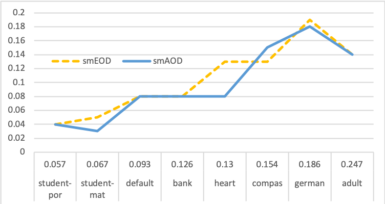
Figure 2: Relationship between the violation of equalized odds of the learned model (measured as smEOD and smAOD at the y-axis) and the corresponding dataset’s difference in class distributions of each demographics (measured as MaxDiff in (29) at the x-axis).

5.1 RQ1 Validate the necessary condition

RQ1 focuses on validating the necessary condition in Proposition 3.3 by empirically analyzing whether the violation of equalized odds of the learned model is positively related to the weighted class distribution differences across each demographic group in the training data. To this end, we plotted the smEOD and smAOD of a logistic regression classifier trained with uniform weights on eight datasets. In Figure 2, x-axis shows the MaxDiff values for each dataset calculated as (29) reflecting the maximum difference in class distributions across each demographic group.

$$\text{MaxDiff}=\max_{a_{i}\in A}\frac{|A=a_{i},Y=1|}{|A=a_{i}|}-\min_{a_{j}\in A}\frac{|A=a_{j},Y=1|}{|A=a_{j}|}.$$ (29)

As we can see from Figure 2, the extent of violation of equalized odds is positively related (not strictly since it is also related to the overall prediction accuracy of the learned model) to the MaxDiff values of the training data. This validates the necessary condition in Proposition 3.3 that the difference in class distributions across each demographic groups lead to the violation of equalized odds.

TABLE III: Model performance with FairBalance on the training data. Each cell shows the median (50th percentile) value, and the IQR value (75th percentile - 25th percentile) of the metric from 30 random repeats on a certain dataset.

Data	Accuracy	AUC	mEOD	mAOD	smEOD	smAOD
Adult	0.82 (0.00)	0.90 (0.00)	0.06 (0.01)	0.02 (0.01)	0.08 (0.01)	0.01 (0.01)
Compas	0.69 (0.01)	0.75 (0.00)	0.08 (0.03)	0.04 (0.02)	0.03 (0.01)	0.02 (0.01)
Heart	0.85 (0.02)	0.93 (0.02)	0.03 (0.03)	0.02 (0.02)	0.03 (0.02)	0.00 (0.00)
Bank	0.85 (0.00)	0.91 (0.00)	0.07 (0.01)	0.00 (0.00)	0.04 (0.01)	0.00 (0.00)
German	0.75 (0.01)	0.84 (0.01)	0.13 (0.07)	0.05 (0.04)	0.09 (0.03)	0.02 (0.02)
Default	0.69 (0.01)	0.72 (0.00)	0.17 (0.02)	0.12 (0.01)	0.01 (0.00)	0.00 (0.00)
Student-por	0.93 (0.02)	0.98 (0.01)	0.02 (0.02)	0.02 (0.02)	0.03 (0.01)	0.00 (0.00)
Student-mat	0.97 (0.01)	1.00 (0.00)	0.03 (0.02)	0.01 (0.01)	0.03 (0.01)	0.00 (0.00)

5.2 RQ2 Validate the sufficient condition

To validate the sufficient condition in Proposition 3.4, we apply FairBalance to multiply the weight $w_{FB}(a_{k},y_{i})$ in (23) to each training data point. As shown in (24), the weighted class distribution in each demographic group becomes balanced after applying the weights. Then we train a logistic regression model on the weighted training data and collect its training performance in Table III. In consistency with the sufficient condition in Proposition 3.4, we can observe that the training smAODs are close to 0 on all eight datasets. The reason for smAODs on the Adult, Compas, and German datasets not strictly being 0 could be that, Assumption 3.2 is not strictly valid for these datasets— all three datasets have two sensitive attributes which can be correlated to each other. On the other hand, the smEODs are not always close to 0 even on the training data.

TABLE IV: Empirical results for RQ3 on the Adult Census Income dataset. Each cell shows (1) the ranking, (2) the median (50th percentile) value, and (3) the IQR value (75th percentile - 25th percentile) of the metric on a certain dataset. Colored cells are the ones with top rank r0.

Treatment	Accuracy	AUC	mEOD	mAOD	smEOD	smAOD	Runtime (secs)
None	r0: 0.85 (0.00)	r0: 0.91 (0.00)	r2: 0.19 (0.10)	r4: 0.14 (0.05)	r2: 0.14 (0.07)	r3: 0.14 (0.04)	r0: 1.18 (0.15)
Reweighing	r1: 0.84 (0.00)	r2: 0.90 (0.00)	r2: 0.17 (0.04)	r3: 0.08 (0.02)	r2: 0.12 (0.05)	r2: 0.04 (0.03)	r0: 1.23 (0.03)
Fair-SMOTE	r4: 0.81 (0.00)	r3: 0.89 (0.00)	r1: 0.07 (0.04)	r1: 0.05 (0.03)	r0: 0.08 (0.03)	r1: 0.03 (0.01)	r3: 142.83 (5.48)
Fair-SMOTE-Situation	r3: 0.81 (0.01)	r2: 0.89 (0.00)	r0: 0.07 (0.04)	r2: 0.06 (0.01)	r0: 0.07 (0.03)	r1: 0.03 (0.02)	r3: 140.52 (14.06)
FairBalance	r2: 0.81 (0.00)	r1: 0.90 (0.00)	r1: 0.08 (0.03)	r0: 0.03 (0.02)	r1: 0.09 (0.03)	r0: 0.02 (0.01)	r1: 1.23 (0.03)
FairBalanceVariant	r3: 0.81 (0.00)	r2: 0.90 (0.00)	r1: 0.08 (0.03)	r1: 0.05 (0.04)	r0: 0.07 (0.03)	r1: 0.03 (0.02)	r2: 1.34 (0.10)

TABLE V: Empirical results for RQ3 on the Compas dataset.

Treatment	Accuracy	AUC	mEOD	mAOD	smEOD	smAOD	Runtime (secs)
None	r0: 0.67 (0.01)	r0: 0.72 (0.01)	r2: 0.23 (0.05)	r2: 0.31 (0.05)	r1: 0.13 (0.02)	r2: 0.15 (0.02)	r0: 0.35 (0.03)
Reweighing	r1: 0.67 (0.01)	r0: 0.72 (0.02)	r1: 0.11 (0.05)	r1: 0.07 (0.05)	r0: 0.03 (0.01)	r0: 0.03 (0.02)	r1: 0.38 (0.04)
Fair-SMOTE	r3: 0.65 (0.01)	r2: 0.70 (0.01)	r0: 0.08 (0.04)	r1: 0.09 (0.05)	r0: 0.03 (0.02)	r1: 0.03 (0.02)	r3: 7.86 (1.15)
Fair-SMOTE-Situation	r3: 0.65 (0.01)	r2: 0.70 (0.01)	r0: 0.07 (0.04)	r1: 0.07 (0.04)	r0: 0.03 (0.01)	r1: 0.03 (0.01)	r2: 6.31 (0.59)
FairBalance	r2: 0.66 (0.00)	r1: 0.72 (0.01)	r0: 0.07 (0.05)	r0: 0.05 (0.04)	r0: 0.03 (0.02)	r0: 0.02 (0.02)	r1: 0.38 (0.05)
FairBalanceVariant	r2: 0.66 (0.01)	r1: 0.71 (0.02)	r1: 0.10 (0.05)	r1: 0.07 (0.06)	r0: 0.03 (0.01)	r0: 0.03 (0.01)	r1: 0.38 (0.04)

TABLE VI: Empirical results for RQ3 on the Heart Health dataset.

Treatment	Accuracy	AUC	mEOD	mAOD	smEOD	smAOD	Runtime (secs)
None	r0: 0.83 (0.05)	r0: 0.90 (0.04)	r1: 0.11 (0.11)	r0: 0.08 (0.08)	r1: 0.13 (0.11)	r0: 0.08 (0.05)	r0: 0.02 (0.00)
Reweighing	r0: 0.84 (0.05)	r0: 0.91 (0.04)	r0: 0.09 (0.13)	r0: 0.08 (0.09)	r0: 0.07 (0.08)	r0: 0.06 (0.07)	r1: 0.02 (0.00)
Fair-SMOTE	r0: 0.81 (0.06)	r0: 0.90 (0.06)	r1: 0.11 (0.12)	r0: 0.05 (0.10)	r0: 0.06 (0.11)	r0: 0.06 (0.07)	r2: 0.14 (0.00)
Fair-SMOTE-Situation	r1: 0.79 (0.03)	r1: 0.88 (0.05)	r0: 0.08 (0.10)	r0: 0.08 (0.13)	r0: 0.05 (0.08)	r0: 0.06 (0.09)	r3: 0.14 (0.00)
FairBalance	r0: 0.83 (0.05)	r0: 0.90 (0.04)	r0: 0.09 (0.10)	r0: 0.07 (0.09)	r0: 0.07 (0.04)	r0: 0.05 (0.06)	r1: 0.02 (0.00)
FairBalanceVariant	r0: 0.83 (0.05)	r0: 0.90 (0.04)	r0: 0.09 (0.10)	r0: 0.06 (0.10)	r0: 0.06 (0.09)	r0: 0.06 (0.07)	r0: 0.02 (0.00)

TABLE VII: Empirical results for RQ3 on the Bank Marketing dataset.

Treatment	Accuracy	AUC	mEOD	mAOD	smEOD	smAOD	Runtime (secs)
None	r0: 0.90 (0.00)	r1: 0.91 (0.00)	r3: 0.13 (0.08)	r2: 0.09 (0.04)	r1: 0.08 (0.03)	r2: 0.08 (0.02)	r0: 0.98 (0.02)
Reweighing	r0: 0.90 (0.00)	r1: 0.90 (0.01)	r2: 0.09 (0.06)	r1: 0.04 (0.03)	r1: 0.08 (0.02)	r1: 0.03 (0.02)	r3: 1.12 (0.02)
Fair-SMOTE	r3: 0.83 (0.01)	r3: 0.89 (0.01)	r0: 0.05 (0.05)	r0: 0.02 (0.03)	r0: 0.03 (0.03)	r0: 0.02 (0.02)	r4: 357.84 (3.24)
Fair-SMOTE-Situation	r2: 0.83 (0.01)	r3: 0.89 (0.01)	r0: 0.06 (0.05)	r0: 0.02 (0.02)	r0: 0.03 (0.03)	r0: 0.01 (0.02)	r4: 357.68 (1.94)
FairBalance	r1: 0.84 (0.00)	r0: 0.91 (0.00)	r1: 0.07 (0.05)	r0: 0.02 (0.02)	r0: 0.04 (0.03)	r0: 0.01 (0.01)	r1: 1.05 (0.02)
FairBalanceVariant	r2: 0.83 (0.00)	r2: 0.90 (0.00)	r0: 0.06 (0.05)	r0: 0.02 (0.02)	r0: 0.04 (0.04)	r0: 0.02 (0.02)	r2: 1.10 (0.02)

TABLE VIII: Empirical results for RQ3 on the German Credit dataset.

Treatment	Accuracy	AUC	mEOD	mAOD	smEOD	smAOD	Runtime (secs)
None	r0: 0.76 (0.03)	r0: 0.79 (0.03)	r2: 0.25 (0.17)	r1: 0.29 (0.16)	r2: 0.19 (0.07)	r1: 0.18 (0.07)	r0: 0.06 (0.00)
Reweighing	r0: 0.75 (0.03)	r0: 0.78 (0.03)	r0: 0.12 (0.08)	r0: 0.16 (0.13)	r0: 0.08 (0.06)	r0: 0.07 (0.05)	r1: 0.07 (0.00)
Fair-SMOTE	r1: 0.71 (0.04)	r1: 0.77 (0.04)	r0: 0.15 (0.12)	r0: 0.19 (0.11)	r1: 0.10 (0.07)	r0: 0.11 (0.06)	r3: 1.85 (0.03)
Fair-SMOTE-Situation	r1: 0.71 (0.03)	r1: 0.77 (0.03)	r1: 0.17 (0.15)	r0: 0.14 (0.10)	r1: 0.10 (0.09)	r0: 0.08 (0.07)	r4: 1.91 (0.03)
FairBalance	r1: 0.72 (0.04)	r0: 0.78 (0.04)	r1: 0.21 (0.16)	r0: 0.15 (0.11)	r1: 0.12 (0.10)	r0: 0.09 (0.06)	r1: 0.07 (0.00)
FairBalanceVariant	r2: 0.70 (0.03)	r1: 0.77 (0.03)	r1: 0.17 (0.16)	r0: 0.18 (0.09)	r1: 0.11 (0.10)	r0: 0.09 (0.05)	r2: 0.07 (0.00)

TABLE IX: Empirical results for RQ3 on the Default of Credit Card Clients dataset.

Treatment	Accuracy	AUC	mEOD	mAOD	smEOD	smAOD	Runtime (secs)
None	r0: 0.81 (0.00)	r0: 0.72 (0.01)	r1: 0.04 (0.01)	r1: 0.06 (0.03)	r3: 0.08 (0.01)	r3: 0.08 (0.02)	r0: 0.68 (0.01)
Reweighing	r0: 0.81 (0.00)	r1: 0.72 (0.00)	r0: 0.01 (0.01)	r0: 0.05 (0.02)	r0: 0.01 (0.01)	r0: 0.01 (0.01)	r1: 0.86 (0.01)
Fair-SMOTE	r2: 0.68 (0.01)	r1: 0.72 (0.01)	r2: 0.16 (0.02)	r2: 0.12 (0.03)	r1: 0.01 (0.00)	r0: 0.01 (0.01)	r3: 611.89 (4.19)
Fair-SMOTE-Situation	r3: 0.61 (0.02)	r1: 0.71 (0.01)	r2: 0.17 (0.07)	r2: 0.12 (0.05)	r2: 0.03 (0.01)	r2: 0.02 (0.01)	r3: 611.01 (2.59)
FairBalance	r1: 0.69 (0.01)	r1: 0.72 (0.01)	r2: 0.17 (0.03)	r2: 0.13 (0.03)	r1: 0.02 (0.01)	r0: 0.01 (0.01)	r1: 0.86 (0.02)
FairBalanceVariant	r2: 0.68 (0.01)	r1: 0.72 (0.01)	r2: 0.16 (0.03)	r2: 0.11 (0.03)	r1: 0.02 (0.01)	r1: 0.02 (0.01)	r2: 0.86 (0.01)

TABLE X: Empirical results for RQ3 on the Student Performance in Portuguese Language dataset.

Treatment	Accuracy	AUC	mEOD	mAOD	smEOD	smAOD	Runtime (secs)
None	r0: 0.92 (0.02)	r0: 0.95 (0.02)	r1: 0.04 (0.02)	r0: 0.05 (0.06)	r2: 0.04 (0.03)	r0: 0.04 (0.03)	r0: 0.05 (0.00)
Reweighing	r0: 0.91 (0.03)	r0: 0.95 (0.02)	r0: 0.02 (0.02)	r0: 0.05 (0.09)	r0: 0.01 (0.02)	r0: 0.04 (0.05)	r2: 0.05 (0.01)
Fair-SMOTE	r1: 0.88 (0.04)	r0: 0.95 (0.02)	r1: 0.03 (0.03)	r0: 0.05 (0.06)	r1: 0.03 (0.06)	r0: 0.05 (0.07)	r3: 0.76 (0.01)
Fair-SMOTE-Situation	r1: 0.88 (0.03)	r1: 0.95 (0.02)	r1: 0.03 (0.04)	r0: 0.06 (0.06)	r1: 0.03 (0.04)	r0: 0.06 (0.06)	r4: 0.79 (0.01)
FairBalance	r1: 0.89 (0.02)	r1: 0.95 (0.02)	r1: 0.04 (0.03)	r0: 0.06 (0.06)	r1: 0.03 (0.04)	r0: 0.05 (0.05)	r2: 0.05 (0.00)
FairBalanceVariant	r1: 0.89 (0.02)	r1: 0.95 (0.01)	r1: 0.04 (0.05)	r0: 0.06 (0.05)	r2: 0.04 (0.04)	r0: 0.06 (0.08)	r1: 0.05 (0.00)

TABLE XI: Empirical results for RQ3 on the Student Performance in Mathematics dataset.

Treatment	Accuracy	AUC	mEOD	mAOD	smEOD	smAOD	Runtime (secs)
None	r0: 0.91 (0.04)	r0: 0.97 (0.01)	r0: 0.05 (0.05)	r0: 0.04 (0.03)	r0: 0.05 (0.03)	r0: 0.03 (0.04)	r0: 0.04 (0.00)
Reweighing	r0: 0.91 (0.03)	r0: 0.97 (0.01)	r0: 0.03 (0.04)	r0: 0.03 (0.04)	r0: 0.03 (0.05)	r0: 0.03 (0.03)	r1: 0.04 (0.00)
Fair-SMOTE	r1: 0.90 (0.04)	r0: 0.97 (0.02)	r1: 0.05 (0.05)	r0: 0.06 (0.07)	r0: 0.06 (0.05)	r0: 0.04 (0.05)	r2: 0.25 (0.00)
Fair-SMOTE-Situation	r1: 0.89 (0.04)	r1: 0.96 (0.02)	r1: 0.05 (0.05)	r0: 0.05 (0.05)	r0: 0.05 (0.06)	r0: 0.03 (0.05)	r3: 0.27 (0.00)
FairBalance	r0: 0.91 (0.03)	r0: 0.98 (0.01)	r0: 0.03 (0.03)	r0: 0.04 (0.04)	r0: 0.04 (0.04)	r0: 0.03 (0.04)	r1: 0.04 (0.00)
FairBalanceVariant	r0: 0.91 (0.03)	r0: 0.97 (0.01)	r1: 0.05 (0.07)	r0: 0.04 (0.06)	r1: 0.06 (0.06)	r0: 0.03 (0.04)	r1: 0.04 (0.00)

TABLE XII: Empirical results for RQ4 on the Adult Census Income dataset.

Treatment	Accuracy	AUC	mEOD	mAOD	smEOD	smAOD	Runtime (secs)
None	r0: 0.85 (0.00)	r0: 0.91 (0.00)	r2: 0.19 (0.10)	r3: 0.14 (0.05)	r2: 0.14 (0.07)	r2: 0.14 (0.04)	r0: 1.27 (0.18)
Fairway	r0: 0.85 (0.00)	r0: 0.91 (0.00)	r2: 0.18 (0.07)	r3: 0.13 (0.03)	r2: 0.12 (0.05)	r2: 0.14 (0.03)	r3: 1.56 (0.05)
FairSituation	r0: 0.85 (0.00)	r0: 0.91 (0.00)	r2: 0.19 (0.11)	r3: 0.14 (0.05)	r2: 0.16 (0.05)	r2: 0.15 (0.03)	r0: 1.30 (0.02)
FairBalance	r1: 0.81 (0.00)	r1: 0.90 (0.00)	r1: 0.08 (0.03)	r0: 0.03 (0.02)	r1: 0.09 (0.03)	r0: 0.02 (0.01)	r1: 1.39 (0.20)
FairBalance+Fairway	r2: 0.80 (0.01)	r1: 0.90 (0.00)	r0: 0.06 (0.03)	r1: 0.04 (0.02)	r0: 0.08 (0.03)	r0: 0.02 (0.01)	r4: 1.78 (0.04)
FairBalance+FairSituation	r2: 0.80 (0.01)	r1: 0.90 (0.00)	r0: 0.07 (0.04)	r2: 0.06 (0.02)	r0: 0.07 (0.02)	r1: 0.03 (0.02)	r2: 1.52 (0.03)

TABLE XIII: Empirical results for RQ4 on the Compas dataset.

Treatment	Accuracy	AUC	mEOD	mAOD	smEOD	smAOD	Runtime (secs)
None	r0: 0.67 (0.01)	r0: 0.72 (0.01)	r3: 0.23 (0.05)	r5: 0.31 (0.05)	r4: 0.13 (0.02)	r3: 0.15 (0.02)	r0: 0.27 (0.01)
Fairway	r1: 0.66 (0.02)	r1: 0.71 (0.02)	r2: 0.18 (0.03)	r3: 0.25 (0.04)	r3: 0.10 (0.02)	r2: 0.13 (0.02)	r4: 0.41 (0.01)
FairSituation	r0: 0.67 (0.01)	r0: 0.72 (0.01)	r3: 0.21 (0.03)	r4: 0.27 (0.05)	r4: 0.12 (0.03)	r3: 0.15 (0.04)	r2: 0.34 (0.01)
FairBalance	r2: 0.66 (0.00)	r1: 0.72 (0.01)	r0: 0.07 (0.05)	r0: 0.05 (0.04)	r0: 0.03 (0.02)	r0: 0.02 (0.02)	r1: 0.31 (0.01)
FairBalance+Fairway	r3: 0.65 (0.01)	r2: 0.71 (0.01)	r1: 0.12 (0.07)	r2: 0.10 (0.03)	r2: 0.06 (0.02)	r1: 0.04 (0.01)	r5: 0.43 (0.01)
FairBalance+FairSituation	r2: 0.66 (0.01)	r1: 0.71 (0.01)	r0: 0.08 (0.06)	r1: 0.07 (0.03)	r1: 0.04 (0.02)	r0: 0.03 (0.01)	r3: 0.38 (0.01)

TABLE XIV: Empirical results for RQ4 on the Heart Health dataset.

Treatment	Accuracy	AUC	mEOD	mAOD	smEOD	smAOD	Runtime (secs)
None	r0: 0.83 (0.05)	r0: 0.90 (0.04)	r1: 0.11 (0.11)	r0: 0.08 (0.08)	r1: 0.13 (0.11)	r0: 0.08 (0.05)	r0: 0.02 (0.00)
Fairway	r0: 0.82 (0.04)	r0: 0.90 (0.03)	r1: 0.11 (0.17)	r1: 0.12 (0.15)	r0: 0.12 (0.10)	r0: 0.08 (0.11)	r3: 0.03 (0.00)
FairSituation	r0: 0.84 (0.03)	r0: 0.90 (0.04)	r0: 0.08 (0.10)	r0: 0.09 (0.10)	r0: 0.07 (0.08)	r0: 0.08 (0.07)	r2: 0.02 (0.00)
FairBalance	r0: 0.83 (0.05)	r0: 0.90 (0.04)	r0: 0.09 (0.10)	r0: 0.07 (0.09)	r0: 0.07 (0.04)	r0: 0.05 (0.06)	r1: 0.02 (0.00)
FairBalance+Fairway	r0: 0.82 (0.05)	r0: 0.89 (0.03)	r0: 0.06 (0.07)	r0: 0.09 (0.06)	r0: 0.07 (0.07)	r0: 0.07 (0.09)	r3: 0.03 (0.00)
FairBalance+FairSituation	r0: 0.82 (0.05)	r0: 0.90 (0.03)	r0: 0.08 (0.11)	r0: 0.08 (0.07)	r0: 0.06 (0.08)	r0: 0.05 (0.06)	r2: 0.02 (0.00)

TABLE XV: Empirical results for RQ4 on the Bank Marketing dataset.

Treatment	Accuracy	AUC	mEOD	mAOD	smEOD	smAOD	Runtime (secs)
None	r0: 0.90 (0.00)	r1: 0.91 (0.00)	r1: 0.13 (0.08)	r1: 0.09 (0.04)	r1: 0.08 (0.03)	r1: 0.08 (0.02)	r0: 0.97 (0.02)
Fairway	r1: 0.90 (0.00)	r2: 0.90 (0.01)	r1: 0.12 (0.06)	r1: 0.08 (0.03)	r1: 0.08 (0.04)	r1: 0.08 (0.02)	r2: 1.27 (0.02)
FairSituation	r1: 0.90 (0.00)	r1: 0.91 (0.00)	r1: 0.12 (0.08)	r1: 0.08 (0.04)	r1: 0.08 (0.05)	r1: 0.08 (0.03)	r2: 1.27 (0.02)
FairBalance	r2: 0.84 (0.00)	r0: 0.91 (0.00)	r0: 0.07 (0.05)	r0: 0.02 (0.02)	r0: 0.04 (0.03)	r0: 0.01 (0.01)	r1: 1.05 (0.02)
FairBalance+Fairway	r4: 0.83 (0.00)	r0: 0.91 (0.00)	r0: 0.08 (0.05)	r0: 0.02 (0.03)	r0: 0.05 (0.03)	r0: 0.02 (0.02)	r3: 1.35 (0.05)
FairBalance+FairSituation	r3: 0.83 (0.00)	r0: 0.91 (0.00)	r0: 0.06 (0.05)	r0: 0.02 (0.02)	r0: 0.05 (0.03)	r0: 0.01 (0.01)	r4: 1.38 (0.03)

TABLE XVI: Empirical results for RQ4 on the German Credit dataset.

Treatment	Accuracy	AUC	mEOD	mAOD	smEOD	smAOD	Runtime (secs)
None	r0: 0.76 (0.03)	r0: 0.79 (0.03)	r1: 0.25 (0.17)	r1: 0.29 (0.16)	r1: 0.19 (0.07)	r2: 0.18 (0.07)	r0: 0.06 (0.00)
Fairway	r0: 0.74 (0.03)	r1: 0.77 (0.05)	r0: 0.21 (0.09)	r1: 0.23 (0.11)	r0: 0.15 (0.07)	r1: 0.13 (0.09)	r4: 0.11 (0.00)
FairSituation	r0: 0.75 (0.02)	r0: 0.78 (0.03)	r1: 0.26 (0.10)	r1: 0.28 (0.12)	r1: 0.18 (0.05)	r2: 0.17 (0.05)	r2: 0.08 (0.00)
FairBalance	r1: 0.72 (0.04)	r0: 0.78 (0.04)	r0: 0.21 (0.16)	r0: 0.15 (0.11)	r0: 0.12 (0.10)	r0: 0.09 (0.06)	r1: 0.07 (0.00)
FairBalance+Fairway	r2: 0.68 (0.02)	r1: 0.75 (0.03)	r0: 0.19 (0.11)	r0: 0.15 (0.11)	r0: 0.13 (0.07)	r0: 0.08 (0.07)	r5: 0.11 (0.00)
FairBalance+FairSituation	r1: 0.70 (0.03)	r0: 0.77 (0.04)	r0: 0.23 (0.16)	r0: 0.15 (0.11)	r0: 0.15 (0.11)	r0: 0.07 (0.09)	r3: 0.09 (0.00)

TABLE XVII: Empirical results for RQ4 on the Default of Credit Card Clients dataset.

Treatment	Accuracy	AUC	mEOD	mAOD	smEOD	smAOD	Runtime (secs)
None	r0: 0.81 (0.00)	r0: 0.72 (0.01)	r0: 0.04 (0.01)	r1: 0.06 (0.03)	r1: 0.08 (0.01)	r1: 0.08 (0.02)	r0: 0.68 (0.01)
Fairway	r2: 0.80 (0.00)	r0: 0.72 (0.01)	r0: 0.04 (0.01)	r0: 0.06 (0.02)	r1: 0.08 (0.01)	r1: 0.08 (0.01)	r2: 0.86 (0.02)
FairSituation	r1: 0.81 (0.00)	r0: 0.72 (0.01)	r0: 0.04 (0.02)	r1: 0.06 (0.02)	r1: 0.08 (0.01)	r1: 0.08 (0.02)	r1: 0.74 (0.01)
FairBalance	r3: 0.69 (0.01)	r1: 0.72 (0.01)	r1: 0.17 (0.03)	r2: 0.13 (0.03)	r0: 0.02 (0.01)	r0: 0.01 (0.01)	r2: 0.85 (0.02)
FairBalance+Fairway	r5: 0.66 (0.00)	r1: 0.72 (0.01)	r2: 0.18 (0.03)	r3: 0.14 (0.03)	r0: 0.01 (0.01)	r0: 0.01 (0.01)	r4: 1.05 (0.02)
FairBalance+FairSituation	r4: 0.67 (0.01)	r0: 0.72 (0.01)	r2: 0.18 (0.02)	r3: 0.13 (0.04)	r0: 0.01 (0.01)	r0: 0.01 (0.01)	r3: 0.94 (0.01)

TABLE XVIII: Empirical results for RQ4 on the Student Performance in Portuguese Language dataset.

Treatment	Accuracy	AUC	mEOD	mAOD	smEOD	smAOD	Runtime (secs)
None	r0: 0.92 (0.02)	r0: 0.95 (0.02)	r0: 0.04 (0.02)	r0: 0.05 (0.06)	r0: 0.04 (0.03)	r0: 0.04 (0.03)	r0: 0.05 (0.00)
Fairway	r0: 0.91 (0.02)	r0: 0.96 (0.02)	r0: 0.02 (0.02)	r0: 0.06 (0.09)	r0: 0.03 (0.02)	r0: 0.05 (0.06)	r4: 0.07 (0.00)
FairSituation	r0: 0.92 (0.02)	r1: 0.95 (0.02)	r0: 0.02 (0.03)	r0: 0.06 (0.06)	r0: 0.03 (0.04)	r0: 0.04 (0.05)	r2: 0.07 (0.00)
FairBalance	r1: 0.89 (0.02)	r1: 0.95 (0.02)	r1: 0.04 (0.03)	r0: 0.06 (0.06)	r0: 0.03 (0.04)	r0: 0.05 (0.05)	r1: 0.05 (0.00)
FairBalance+Fairway	r1: 0.89 (0.04)	r1: 0.94 (0.03)	r1: 0.04 (0.04)	r0: 0.05 (0.05)	r0: 0.04 (0.04)	r0: 0.05 (0.04)	r5: 0.08 (0.00)
FairBalance+FairSituation	r1: 0.89 (0.02)	r1: 0.95 (0.02)	r1: 0.06 (0.07)	r0: 0.09 (0.06)	r0: 0.05 (0.05)	r0: 0.06 (0.06)	r3: 0.07 (0.00)

TABLE XIX: Empirical results for RQ4 on the Student Performance in Mathematics dataset.

Treatment	Accuracy	AUC	mEOD	mAOD	smEOD	smAOD	Runtime (secs)
None	r0: 0.91 (0.04)	r0: 0.97 (0.01)	r0: 0.05 (0.05)	r0: 0.04 (0.03)	r0: 0.05 (0.03)	r0: 0.03 (0.04)	r0: 0.04 (0.00)
Fairway	r1: 0.89 (0.04)	r1: 0.96 (0.02)	r0: 0.05 (0.07)	r0: 0.05 (0.05)	r1: 0.05 (0.04)	r0: 0.03 (0.05)	r4: 0.06 (0.00)
FairSituation	r0: 0.91 (0.03)	r0: 0.97 (0.02)	r1: 0.08 (0.07)	r1: 0.06 (0.04)	r1: 0.07 (0.06)	r0: 0.05 (0.02)	r2: 0.06 (0.00)
FairBalance	r0: 0.91 (0.03)	r0: 0.98 (0.01)	r0: 0.03 (0.03)	r0: 0.04 (0.04)	r0: 0.04 (0.04)	r0: 0.03 (0.04)	r1: 0.04 (0.00)
FairBalance+Fairway	r1: 0.88 (0.04)	r1: 0.96 (0.02)	r1: 0.08 (0.08)	r0: 0.06 (0.09)	r1: 0.06 (0.06)	r0: 0.03 (0.04)	r5: 0.06 (0.00)
FairBalance+FairSituation	r1: 0.90 (0.03)	r0: 0.97 (0.01)	r1: 0.05 (0.08)	r0: 0.04 (0.03)	r0: 0.05 (0.06)	r0: 0.04 (0.04)	r3: 0.06 (0.00)

5.3 RQ3 Category 3 pre-processing

RQ3 tests the proposed pre-processing algorithms FairBalance and FairBalanceVariant against the state-of-the-art Category 3 pre-processing algorithms Reweighing [12], Fair-SMOTE [10], and Fair-SMOTE-Situation [10]. Here, Fair-SMOTE-Situation is the combination of Fair-SMOTE and FairSituation. According to Chakraborty et al. [10] it first applies Fair-SMOTE to generate synthetic data points so that the training data is balanced as (26), then it applies FairSituation to remove data points failing the situation testing from the training data. Each treatment is evaluated 30 times during the experiments by each time randomly sampling 70% of the data as training set and the rest as test set. Performances of each treatment on the test set are shown in Table IV-XI. From these tables, we can observe:

• On most datasets (except for the Math dataset where the MaxDiff is close to 0 in Figure 2), equalized odds (measured by smEOD and smAOD) of the None treatment can be significantly improved after applying any of the pre-processing treatment. This aligns with the analysis that all these pre-processing treatments satisfy the necessary condition in Proposition 3.3.

• FairBalance always achieves the best smAOD (ranked as r0) on every dataset. Following that, FairBalanceVariant and Fair-SMOTE are ranked r0 on 6 datasets and r1 on 2 datasets. Reweighing is ranked r0 on 6 datasets, r1 on the Bank Marketing dataset and r2 on the Adult Census Income dataset. Such results align with the analysis that FairBalance, FairBalanceVariant, and Fair-SMOTE satisfy the sufficient condition in Proposition 3.4 which leads to better smAOD.

• In terms of smEOD, Reweighing (6 r0, 1 r1, and 1 r2) and Fair-SMOTE (5 r0 and 3 r1) outperform FairBalance (4 r0 and 4 r1) and the other algorithms.

• In terms of utility, FairBalance (4 r0 and 4 r1) and Reweighing (5 r0, 2 r1, and 1 r2) achieves the best AUC amongst the six treatments.

• In terms of runtime, FairBalance, FairBalanceVariant, and Reweighing have similar computational overheads (5-25%), while Fair-SMOTE and Fair-SMOTE-Situation have much higher computational overheads.

Overall, the empirical results on the eight real world datasets are consistent with our analyses in Section 3. Among the five tested pre-processing algorithms, we would recommend FairBalance since (1) it always achieves the best smAOD, (2) in terms of utility measured by AUC, it is also one of the best treatments, (3) it also has very small computational overhead. Note that, when smEOD and smAOD cannot be both satisfied, we value smAOD more since it is a more comprehensive metric (reflecting both the difference in true positive rate and false positive rate) than smEOD (which only relfects the difference in true positive rate). Note that, FairBalance achieves higher smAODs on the test sets than the training sets. This is due to the sampling bias which causes the training and test set not strictly following the same distribution. This is especially obvious on smaller datasets such as Heart, German, Student-Portuguese, and Student-Mathematics with $\leq$1,000 samples.

5.4 RQ4 Category 2 pre-processing

RQ3 has shown that FairBalance is the best Category 3 pre-processing algorithm for smAOD and AUC. Inspired by the ensemble algorithms such as Chakraborty et al. [10], RQ4 tests how the Category 2 algorithms affect equalized odds and whether they can further improve the model’s performance when applied in combination with FairBalance. Performances of each treatment on the test set are shown in Table XII-XIX. From these tables, we can observe:

• Fairway and FairSituation cannot achieve comparable smAOD or smEOD with FairBalance on most of the datasets (5 out of 8). They do not have much improvement smAOD or smEOD over the None treatment either. Fairway only slightly improves smAOD and smEOD over the None treatment on 3 out of 8 datasets and FairSituation does so on only 1 dataset. This is consistent with our analysis since Fairway and FairSituation do not satisfy the necessary condition in Proposition 3.3.

• Adding either Fairway of FairSituation to FairBalance only worthen the smAOD performance on at least one dataset. Both FairBalance+Fairway of FairBalance+FairSituation do not improve on other metrics such as AUC or smEOD comparing to just applying FairBalance.

Overall, the Category 2 pre-processing algorithms do not improve equalized odds and there is little value in applying FairBalance along with them.

6 Threats to validity

Sampling Bias - Logistic regression model is used as the base classifier and eight real world datasets are used for the experiments. Conclusions may change if other datasets and classification models are used. Specifically, Zhang and Harman [66] showed that enlarging feature set of the data could improve both fairness and accuracy.
Evaluation Bias - We focused on the equalized odds fairness notion and evaluated it with smEOD and smAOD.
Conclusion Validity - Analyses in this work were made based on Assumption 3.1 and 3.2. Prior fairness studies made similar assumptions [10, 67]. However, such assumptions may not always hold for data with human decisions.
External Validity - This work focuses on classification problems which are very common in AI software. We are currently working on extending it to regression problems.

7 Conclusion

This paper aims to improve equalized odds fairness notion of classifiers by assigning different weights to the training data points. Our first finding is that, equal weighted class distributions across each demographic group is a necessary condition for equalized odds (Proposition 3.3). This is also validated empirically in RQ1 where we showed the extent of violation of equalized odds is positively related to the max difference in the class distributions, and that in RQ3 and RQ4, the pre-processing algorithms satisfying the necessary condition achieve better equalized odds than those do not. The second finding is, when the weighted class distributions are balanced (1:1) in every demographic group, partial equalized odds (smAOD=0) can be guaranteed in the training data (Proposition 3.4). This sufficient condition is empirically validated in RQ2 that with FairBalance balancing the training data, smAODs are close to 0 on every training datasets. Note that these two major findings are subject to Assumption 3.1 and 3.2 in Section 3. They also hold for any unbiased predictors with zero mean of training errors and an intercept term.

With the two findings, we proposed FairBalance, a pre-processing algorithm balancing the training data. With experiments on eight real world datasets, we show in RQ3 and RQ4 that FairBalance outperforms every other baseline in smAOD, and is on par with them in terms of utility (measured by AUC) and runtime. Also note that, FairBalance is model-agnostic itself, but the theoretical guarantee for achieving good smAOD is limited to unbiased predictors. Overall, we would recommend FairBalance when building a classification software satisfying equalized odds.

Given the threats to validity discussed in Section 6 and the above limitations of the work, future work of this paper will focus on:

• How to detect and mitigate biased labels. Equalized odds is no longer reliable when ground truth labels can be biased. But this also creates an opportunity to isolate the bias inherited from the training data when applying FairBalance to mitigate the bias originated from the training process. When equalized odds is violated for a model trained with FairBalance, the violation is possibly due to the biased labels.

• How to mitigate potential ethical bias when the sensitive attributes are unknown or noisy. There are some existing work along this research [68], However, it remains as a major challenge for machine learning fairness.

• How to generalize this work to regression problems when the dependent variable and the sensitive attributes can be continuous. This requires a generalized definition of equalized odds for the regression problems.

Zhe Yu (Ph.D. NC State University, 2020) is an assistant professor in the Department of Software Engineering at Rochester Institute of Technology, where he teaches data mining and software engineering. His research explores collaborations of human and machine learning algorithms that leads to better performance and higher efficiency. For more information, please visit http://zhe-yu.github.io/.

Joymallya Chakraborty is an Applied Scientist II at Amazon in Seattle. He completed his Ph.D. in Computer Science from North Carolina State University. His research interests include algorithmic bias, ML model optimization, interpretability & explanation of black-box ML models. To know more about him, please visit https://joymallyac.github.io/

Tim Menzies (IEEE Fellow) is a Professor in CS at NcState His research interests include software engineering (SE), data mining, artificial intelligence, search-based SE, and open access science. http://menzies.us

References

- [1] A. Kharpal, “Health care start-up says a.i. can diagnose patients better than humans can, doctors call that ’dubious’,” https://www.cnbc.com/2018/06/28/babylon-claims-its-ai-can-diagnose-patients-better-than-doctors.html, June 2018.
- [2] E. Strickland, “Doc bot preps for the o.r.” IEEE Spectrum, vol. 53, no. 6, pp. 32–60, June 2016.
- [3] P. Olson, “The algorithm that beats your bank manager,” https://www.forbes.com/sites/parmyolson/2011/03/15/the-algorithm-that-beats-your-bank-manager/##15da2651ae99, 2011.
- [4] J. Angwin, J. Larson, S. Mattu, and L. Kirchner, “Machine bias: There’s software used across the country to predict future criminals. and it’s biased against blacks,” https://www.propublica.org/article/machine-bias-risk-assessments-in-criminal-sentencing, 2016.
- [5] J. Dastin, “Amazon scraps secret ai recruiting tool that showed bias against women,” 2018. [Online]. Available: https://www.reuters.com/article/us-amazon-com-jobs-automation-insight/amazon-scraps-secret-ai-recruiting-tool-that-showed-bias-against-women-idUSKCN1MK08G
- [6] S. Verma and J. Rubin, “Fairness definitions explained,” in Proceedings of the international workshop on software fairness, 2018, pp. 1–7.
- [7] N. Mehrabi, F. Morstatter, N. Saxena, K. Lerman, and A. Galstyan, “A survey on bias and fairness in machine learning,” ACM Computing Surveys (CSUR), vol. 54, no. 6, pp. 1–35, 2021.
- [8] M. Hardt, E. Price, and N. Srebro, “Equality of opportunity in supervised learning,” Advances in neural information processing systems, vol. 29, 2016.
- [9] J. Chakraborty, S. Majumder, Z. Yu, and T. Menzies, “Fairway: a way to build fair ml software,” in Proceedings of the 28th ACM Joint Meeting on European Software Engineering Conference and Symposium on the Foundations of Software Engineering, 2020, pp. 654–665.
- [10] J. Chakraborty, S. Majumder, and T. Menzies, “Bias in machine learning software: Why? how? what to do?” in Proceedings of the 29th ACM Joint Meeting on European Software Engineering Conference and Symposium on the Foundations of Software Engineering, ser. ESEC/FSE 2021. New York, NY, USA: Association for Computing Machinery, 2021, p. 429–440. [Online]. Available: https://doi.org/10.1145/3468264.3468537
- [11] K. Peng, J. Chakraborty, and T. Menzies, “Fairmask: Better fairness via model-based rebalancing of protected attributes,” IEEE Transactions on Software Engineering, 2022.
- [12] F. Kamiran and T. Calders, “Data preprocessing techniques for classification without discrimination,” Knowledge and Information Systems, vol. 33, no. 1, pp. 1–33, 2012.
- [13] F. P. Calmon, D. Wei, B. Vinzamuri, K. N. Ramamurthy, and K. R. Varshney, “Optimized pre-processing for discrimination prevention,” in Proceedings of the 31st International Conference on Neural Information Processing Systems, 2017, pp. 3995–4004.
- [14] B. H. Zhang, B. Lemoine, and M. Mitchell, “Mitigating unwanted biases with adversarial learning,” in Proceedings of the 2018 AAAI/ACM Conference on AI, Ethics, and Society, 2018, pp. 335–340.
- [15] A. Lowy, R. Pavan, S. Baharlouei, M. Razaviyayn, and A. Beirami, “Fermi: Fair empirical risk minimization via exponential renyi mutual information,” arXiv preprint arXiv:2102.12586, 2021.
- [16] P. Li and H. Liu, “Achieving fairness at no utility cost via data reweighing with influence,” in International Conference on Machine Learning. PMLR, 2022, pp. 12 917–12 930.
- [17] “Ethically-aligned design: A vision for prioritizing human well-begin with autonomous and intelligence systems.” 2019.
- [18] “Ethics guidelines for trustworthy artificial intelligence.” 2018. [Online]. Available: https://ec.europa.eu/digital-single-market/en/news/ethics-guidelines-trustworthy-ai
- [19] “Microsoft ai principles. 2019.” 2019. [Online]. Available: https://www.microsoft.com/en-us/ai/our-approach-to-ai
- [20] R. K. E. Bellamy, K. Dey, M. Hind, S. C. Hoffman, S. Houde, K. Kannan, P. Lohia, J. Martino, S. Mehta, A. Mojsilovic, S. Nagar, K. N. Ramamurthy, J. Richards, D. Saha, P. Sattigeri, M. Singh, K. R. Varshney, and Y. Zhang, “AI Fairness 360: An extensible toolkit for detecting, understanding, and mitigating unwanted algorithmic bias,” Oct. 2018. [Online]. Available: https://arxiv.org/abs/1810.01943
- [21] “Fate: Fairness, accountability, transparency, and ethics in ai,” 2018. [Online]. Available: https://www.microsoft.com/en-us/research/group/fate/
- [22] D. Gershgorn, “Facebook says it has a tool to detect bias in its artificial intelligence,” 2018. [Online]. Available: https://qz.com/1268520/facebook-says-it-has-a-tool-to-detect-bias-in-its-artificial-intelligence/
- [23] “Explain 2019.” [Online]. Available: https://2019.ase-conferences.org/home/explain-2019
- [24] S. Sharma, Y. Zhang, J. M. Ríos Aliaga, D. Bouneffouf, V. Muthusamy, and K. R. Varshney, “Data augmentation for discrimination prevention and bias disambiguation,” in Proceedings of the AAAI/ACM Conference on AI, Ethics, and Society, 2020, pp. 358–364.
- [25] E. Black, S. Yeom, and M. Fredrikson, “Fliptest: fairness testing via optimal transport,” in Proceedings of the 2020 Conference on Fairness, Accountability, and Transparency, 2020, pp. 111–121.
- [26] H. Zheng, Z. Chen, T. Du, X. Zhang, Y. Cheng, S. Ji, J. Wang, Y. Yu, and J. Chen, “Neuronfair: Interpretable white-box fairness testing through biased neuron identification,” in Proceedings of the 44th International Conference on Software Engineering, 2022, pp. 1519–1531.
- [27] P. Zhang, J. Wang, J. Sun, G. Dong, X. Wang, X. Wang, J. S. Dong, and T. Dai, “White-box fairness testing through adversarial sampling,” in Proceedings of the ACM/IEEE 42nd International Conference on Software Engineering, 2020, pp. 949–960.
- [28] L. Zhang, Y. Zhang, and M. Zhang, “Efficient white-box fairness testing through gradient search,” in Proceedings of the 30th ACM SIGSOFT International Symposium on Software Testing and Analysis, 2021, pp. 103–114.
- [29] Z. Jiang, X. Han, C. Fan, F. Yang, A. Mostafavi, and X. Hu, “Generalized demographic parity for group fairness,” in International Conference on Learning Representations, 2022.
- [30] J. Zhang and E. Bareinboim, “Equality of opportunity in classification: A causal approach,” Advances in neural information processing systems, vol. 31, 2018.
- [31] G. Pleiss, M. Raghavan, F. Wu, J. Kleinberg, and K. Q. Weinberger, “On fairness and calibration,” 2017.
- [32] J. R. Foulds, R. Islam, K. N. Keya, and S. Pan, “Bayesian modeling of intersectional fairness: The variance of bias,” in Proceedings of the 2020 SIAM International Conference on Data Mining. SIAM, 2020, pp. 424–432.
- [33] M. Feldman, S. A. Friedler, J. Moeller, C. Scheidegger, and S. Venkatasubramanian, “Certifying and removing disparate impact,” in proceedings of the 21th ACM SIGKDD international conference on knowledge discovery and data mining, 2015, pp. 259–268.
- [34] F. Calmon, D. Wei, B. Vinzamuri, K. Natesan Ramamurthy, and K. R. Varshney, “Optimized pre-processing for discrimination prevention,” in Advances in Neural Information Processing Systems 30, I. Guyon, U. V. Luxburg, S. Bengio, H. Wallach, R. Fergus, S. Vishwanathan, and R. Garnett, Eds. Curran Associates, Inc., 2017, pp. 3992–4001. [Online]. Available: http://papers.nips.cc/paper/6988-optimized-pre-processing-for-discrimination-prevention.pdf
- [35] R. Zemel, Y. Wu, K. Swersky, T. Pitassi, and C. Dwork, “Learning fair representations,” in International conference on machine learning. PMLR, 2013, pp. 325–333.
- [36] Y. Romano, S. Bates, and E. Candes, “Achieving equalized odds by resampling sensitive attributes,” Advances in neural information processing systems, vol. 33, pp. 361–371, 2020.
- [37] N. V. Chawla, K. W. Bowyer, L. O. Hall, and W. P. Kegelmeyer, “Smote: synthetic minority over-sampling technique,” Journal of artificial intelligence research, vol. 16, pp. 321–357, 2002.
- [38] S. Yan, H.-t. Kao, and E. Ferrara, “Fair class balancing: Enhancing model fairness without observing sensitive attributes,” in Proceedings of the 29th ACM International Conference on Information & Knowledge Management, 2020, pp. 1715–1724.
- [39] L. E. Celis, L. Huang, V. Keswani, and N. K. Vishnoi, “Classification with fairness constraints: A meta-algorithm with provable guarantees,” in Proceedings of the conference on fairness, accountability, and transparency, 2019, pp. 319–328.
- [40] T. Kamishima, S. Akaho, H. Asoh, and J. Sakuma, “Fairness-aware classifier with prejudice remover regularizer,” in Machine Learning and Knowledge Discovery in Databases, P. A. Flach, T. De Bie, and N. Cristianini, Eds. Berlin, Heidelberg: Springer Berlin Heidelberg, 2012, pp. 35–50.
- [41] M. B. Zafar, I. Valera, M. Gomez Rodriguez, and K. P. Gummadi, “Fairness beyond disparate treatment & disparate impact: Learning classification without disparate mistreatment,” in Proceedings of the 26th international conference on world wide web, 2017, pp. 1171–1180.
- [42] A. Agarwal, A. Beygelzimer, M. Dudík, J. Langford, and H. Wallach, “A reductions approach to fair classification,” in International Conference on Machine Learning. PMLR, 2018, pp. 60–69.
- [43] P. S. Thomas, B. Castro da Silva, A. G. Barto, S. Giguere, Y. Brun, and E. Brunskill, “Preventing undesirable behavior of intelligent machines,” Science, vol. 366, no. 6468, pp. 999–1004, 2019.
- [44] M. Kearns, S. Neel, A. Roth, and Z. S. Wu, “Preventing fairness gerrymandering: Auditing and learning for subgroup fairness,” in International conference on machine learning. PMLR, 2018, pp. 2564–2572.
- [45] X. Gao, J. Zhai, S. Ma, C. Shen, Y. Chen, and Q. Wang, “Fairneuron: improving deep neural network fairness with adversary games on selective neurons,” in Proceedings of the 44th International Conference on Software Engineering, 2022, pp. 921–933.
- [46] F. Kamiran, S. Mansha, A. Karim, and X. Zhang, “Exploiting reject option in classification for social discrimination control,” Inf. Sci., 2018.
- [47] P. Awasthi, M. Kleindessner, and J. Morgenstern, “Equalized odds postprocessing under imperfect group information,” in International conference on artificial intelligence and statistics. PMLR, 2020, pp. 1770–1780.
- [48] M. Hort, J. M. Zhang, F. Sarro, and M. Harman, “Fairea: A model behaviour mutation approach to benchmarking bias mitigation methods,” in Proceedings of the 29th ACM Joint Meeting on European Software Engineering Conference and Symposium on the Foundations of Software Engineering, 2021, pp. 994–1006.
- [49] D. Bhaskaruni, H. Hu, and C. Lan, “Improving prediction fairness via model ensemble,” in 2019 IEEE 31st International Conference on Tools with Artificial Intelligence (ICTAI). IEEE, 2019, pp. 1810–1814.
- [50] V. Iosifidis, B. Fetahu, and E. Ntoutsi, “Fae: A fairness-aware ensemble framework,” in 2019 IEEE International Conference on Big Data (Big Data). IEEE, 2019, pp. 1375–1380.
- [51] P. J. Kenfack, A. M. Khan, S. A. Kazmi, R. Hussain, A. Oracevic, and A. M. Khattak, “Impact of model ensemble on the fairness of classifiers in machine learning,” in 2021 International Conference on Applied Artificial Intelligence (ICAPAI). IEEE, 2021, pp. 1–6.
- [52] Z. Chen, J. M. Zhang, F. Sarro, and M. Harman, “Maat: a novel ensemble approach to addressing fairness and performance bugs for machine learning software,” in Proceedings of the 30th ACM Joint European Software Engineering Conference and Symposium on the Foundations of Software Engineering, 2022, pp. 1122–1134.
- [53] S. Biswas and H. Rajan, “Fair preprocessing: towards understanding compositional fairness of data transformers in machine learning pipeline,” in Proceedings of the 29th ACM Joint Meeting on European Software Engineering Conference and Symposium on the Foundations of Software Engineering, 2021, pp. 981–993.
- [54] “Uci: Adult data set,” 1994. [Online]. Available: http://mlr.cs.umass.edu/ml/datasets/Adult
- [55] “propublica/compas-analysis,” 2015. [Online]. Available: https://github.com/propublica/compas-analysis
- [56] “Uci: Heart disease data set,” 2001. [Online]. Available: https://archive.ics.uci.edu/ml/datasets/Heart+Disease
- [57] “Uci: Bank marketing data set,” 2017. [Online]. Available: https://www.kaggle.com/c/bank-marketing-uci
- [58] “Uci: German credit data set,” 1994. [Online]. Available: https://archive.ics.uci.edu/ml/datasets/statlog+(german+credit+data)
- [59] “Uci: Default of credit card clients data set,” 2016. [Online]. Available: https://archive.ics.uci.edu/ml/datasets/default+of+credit+card+clients
- [60] “Uci: Student performance data set,” 2017. [Online]. Available: https://archive.ics.uci.edu/ml/datasets/student%2Bperformance
- [61] J. Chakraborty, K. Peng, and T. Menzies, “Making fair ml software using trustworthy explanation,” in Proceedings of the 35th IEEE/ACM International Conference on Automated Software Engineering, ser. ASE ’20. New York, NY, USA: Association for Computing Machinery, 2020, p. 1229–1233. [Online]. Available: https://doi.org/10.1145/3324884.3418932
- [62] D. Dua and C. Graff, “UCI machine learning repository,” 2017. [Online]. Available: http://archive.ics.uci.edu/ml
- [63] H. B. Mann and D. R. Whitney, “On a test of whether one of two random variables is stochastically larger than the other,” The annals of mathematical statistics, pp. 50–60, 1947.
- [64] N. Cliff, “Dominance statistics: Ordinal analyses to answer ordinal questions.” Psychological bulletin, vol. 114, no. 3, p. 494, 1993.
- [65] A. J. Scott and M. Knott, “A cluster analysis method for grouping means in the analysis of variance,” Biometrics, pp. 507–512, 1974.
- [66] J. M. Zhang and M. Harman, “" ignorance and prejudice" in software fairness,” in 2021 IEEE/ACM 43rd International Conference on Software Engineering (ICSE). IEEE, 2021, pp. 1436–1447.
- [67] S. Biswas and H. Rajan, “Do the machine learning models on a crowd sourced platform exhibit bias? an empirical study on model fairness,” Proceedings of the 28th ACM Joint Meeting on European Software Engineering Conference and Symposium on the Foundations of Software Engineering, Nov 2020. [Online]. Available: http://dx.doi.org/10.1145/3368089.3409704
- [68] S. Wang, W. Guo, H. Narasimhan, A. Cotter, M. Gupta, and M. I. Jordan, “Robust optimization for fairness with noisy protected groups,” arXiv preprint arXiv:2002.09343, 2020.