Operator growth in the transverse-field Ising spin chain with integrability-breaking longitudinal field

Abstract

We investigate the operator growth dynamics of the transverse field Ising spin chain in one dimension as varying the strength of the longitudinal field. An operator in the Heisenberg picture spreads in the extended Hilbert space. Recently, it has been proposed that the spreading dynamics has a universal feature signaling chaoticity of underlying quantum dynamics. We demonstrate numerically that the operator growth dynamics in the presence of the longitudinal field follows the universal scaling law for one-dimensional chaotic systems. We also find that the operator growth dynamics satisfies a crossover scaling law when the longitudinal field is weak. The crossover scaling confirms that the uniform longitudinal field makes the system chaotic at any nonzero value. We also discuss the implication of the crossover scaling on the thermalization dynamics and the effect of a nonuniform local longitudinal field.

I introduction

There is growing interest in the theory for emergence of equilibrium statistical mechanics in isolated quantum systems [1]. The canonical typicality [2], a reincarnation of the quantum ergodic theory [3, 4], assumes that a Hamiltonian eigenstate is statistically equivalent to a typical state in the Hilbert space, so a quantum mechanical expectation value of a local quantity is indistinguishable from the statistical ensemble average. The eigenstate thermalization hypothesis [5] makes an explicit and testable ansatz for matrix elements of a local observable in the Hamiltonian eigenstate basis to ensure the quantum thermalization. Extensive numerical works have been performed to examine the ansatz directly (see Ref. [1] and references therein) and its thermodynamic implications on e.g. the fluctuation-dissipation theorem [6, 7, 8, 9].

Dynamical aspects of the quantum thermalization have also been attracting a growing interest. For example, out-of-time-ordered correlations have been studied with the hope to uncover a chaotic signature of quantum dynamics [10, 11, 12, 13, 14]. More recently, researchers gained insight into the quantum chaos from the operator growth dynamics. Quantum mechanics can be formulated in terms of the time evolution of an operator in the Heisenberg picture. An operator, initially local and simple, becomes nonlocal and complex as it evolves in time, spreading in the operator Hilbert space. By quantifying and characterizing the complexity of the operator growth dynamics, one may have a better understanding of quantum chaos and equilibration dynamics of isolated quantum systems [15, 16, 17, 18, 19, 20, 21].

The operator growth dynamics is intrinsically limited by an upper bound set by the spatial dimensionality and locality of interactions. Parker et al. proposed a hypothesis that the operator growth dynamics in nonintegrable systems follows a universal scaling law corresponding to the maximal growth [17]. The hypothesis is supported by analytic and numerical calculations on the Sachdev-Ye-Kitaev (SYK) model, which is defined in the infinite-dimensional space. Numerical results on low-dimensional systems seem to be consistent with the hypothesis, but more extensive studies are necessary for a decisive conclusion.

In this paper, we investigate numerically the operator growth dynamics in the transverse field Ising (t-Ising) spin chain in one dimension in the presence or absence of a longitudinal field. The system is useful since one can control the integrability by varying the longitudinal field [22]. We will show that the operator growth dynamics follows the universal scaling law predicted in Ref. [17]. The spatial structure of the one dimensional lattice gives rise to a logarithmic correction in the operator growth dynamics, which is absent in higher dimensional systems. Our results demonstrate the presence of the logarithmic correction. It supports that the universal operator growth hypothesis [17] is valid in low-dimensional systems. We will also show that the operator growth dynamics is an extremely useful tool for investigating the transition from integrability to nonintegrability. The system displays an interesting crossover as one turns on the uniform longitudinal field. Using the crossover, we will show that the system is thermal at any nonzero value of the longitudinal field. As a byproduct, the crossover also reveals the scaling property of the thermalization dynamics [23, 24, 25, 26, 27, 28, 29], which will be detailed in Sec. IV.

The paper is organized as follows: In Sec. II, we present the review on the operator growth dynamics. The universal feature of the operator growth dynamics in some solvable models is summarized in Sec. III. We present our main results for the transverse field Ising spin chain in Sec. IV. Summary and discussions are given in Sec. V.

II Operator growth dynamics

We consider a system with Hamiltonian $H$ acting on the $D$ dimensional Hilbert space. Focusing on operators instead of state vectors, one can formulate the quantum mechanics with the von Neumann equation

$$\frac{\partial}{\partial t}O(t)=i\mathcal{L}O(t)$$ (1)

for an operator $O(t)$ in the Heisenberg picture. Here, $\mathcal{L}$ is the Liouvillian superoperator defined as

$$\mathcal{L}A=[H,A]$$ (2)

with $\hbar=1$. One can introduce an inner product between two operators. Then, an operator $O(t)$ can be regarded as a state vector, denoted as $|O(t))$ , in the operator Hilbert space of dimensionality $D^{2}$. Under this point of view, the quantum mechanical dynamics describes the spreading or growth of an initial state $|O(0))$ in the extended operator Hilbert space.

The operator growth is described conveniently with the Krylov basis. An initial state $|O)$ spreads within the subspace spanned by $\{|O),\mathcal{L}|O),,\cdots\,\mathcal{L}^{n}|O),\cdots\}$, called the Krylov subspace. The orthonormal basis set $\{|O_{0}),|O_{1}),\cdots,|O_{n}),\cdots\}$ can be constructed recursively using the Gram-Schmidt method. It starts with the normalized initial state $|O_{0})=|O)/\sqrt{(O|O)}$ and proceeds to generate the successive basis states via the recursion relations

$$|A_{n}) =\mathcal{L}|O_{n-1})-b_{n-1}|O_{n-2})$$ (3)

$$|O_{n}) =\frac{1}{b_{n}}|A_{n})\mbox{ with }b_{n}=\sqrt{(A_{n}|A_{n})}$$

for $n\geq 1$. The operator inner product can be chosen as

$$(A|B)\equiv\frac{1}{D}{\rm Tr}\left[A^{\dagger}B\right].$$ (4)

It is the infinite temperature average of $A^{\dagger}B$. One may adopt a different choice of the inner product [17, 18]. In this paper, however, we will take the simplest choice of Eq. (4).

This procedure, which is usually referred to as the Lanczos algorithm [31], results in the Krylov basis set and also the sequence $\{b_{n}\}$, called the Lanczos coefficient with $b_{0}=0$. In computational science, the Lanczos algorithm is one of the most important numerical methods with which one can reduce a Hermitian matrix to a tridiagonal form. It also underlies the recursion method which is a useful technique for evaluating the correlation functions in condensed matter physics. For thorough reviews, we refer the readers to Ref. [32].

Recently, Parker et al. attempted to use the Lanczos algorithm to characterize the operator growth dynamics [17]. An operator at time $t$ is written as

$$|O(t))=e^{i\mathcal{L}t}|O_{0})=\sum_{n=0}^{\infty}\varphi_{n}(t)|O_{n}),$$ (5)

where $\varphi_{n}(t)=(O_{n}|O(t))$ is the probability amplitude to be in the $n$th Krylov state. The Liouvillian operator is represented as a tridiagonal matrix $L_{m,n}=(O_{m}|\mathcal{L}|O_{n})$ with $\mathcal{L}_{n,n-1}=\mathcal{L}_{n-1,n}=b_{n}$ and $\mathcal{L}_{n,m}=0$ for $|n-m|\neq 1$. Thus, the probability amplitudes satisfy the discrete Schrödinger equation

$$\dot{\varphi}_{n}(t)=b_{n}\varphi_{n-1}-b_{n+1}\varphi_{n+1}$$ (6)

with the initial condition $\varphi_{n}(0)=\delta_{n0}$ and $b_{0}=0$. Among all {$\varphi_{n}(t)$}, $\varphi_{0}(t)$ is equal to the autocorrelation function $C_{O}(t)=(O|O(t))$. The Schrödinger equation in Eq. (6) describes a tight-binding system in a semi-infinite one-dimensional lattice with coordinate $n$, which will be called a depth in the Krylov space. Parker et al. showed that the Lanczos coefficient is bounded above for systems with local interactions in a $d$ dimensional space. The bounds are

$$b_{n}=\left\{\begin{aligned} &O(n/\ln n)\quad\mbox{ for }d=1\\ &O(n)\quad\mbox{ for }d>1.\end{aligned}\right.$$ (7)

When the bound is achieved, the average depth $n_{t}\equiv\sum_{n}n|\varphi_{n}(t)|^{2}$ grows fastest in time. That is, $n_{t}$ grows exponentially in time when $b_{n}\propto n$, which signals the chaotic nature of quantum dynamics. Based on these observations and known results of solvable systems, they hypothesize that the quantum systems are chaotic only when the Lanczos coefficient follows the scaling law in Eq. (7) [17]. There also exists a rigorous work on the lower bound for $\{b_{n}\}$ for a specific class of systems including the chaotic Ising spin chain [33].

III Solvable systems

Table 1: Lanczos coefficients and the autocorrelation function in exactly solvable cases. $(\eta)_{n}=\eta(\eta+1)\cdots(\eta+n-1)$ is the Pochhammer symbol.

	$b_{n}$	$C(t)$	$\varphi_{n}(t)$	$(n)_{t}=\sum_{n}n|\varphi_{n}(t)|^{2}$
Type I	$\alpha$	$J_{1}(2\alpha t)/(\alpha t)$	$(n+1)J_{n+1}(2\alpha t)/(\alpha t)$	$\frac{16}{3\pi}\alpha t+o(t)$
Type II	$\alpha\sqrt{n}$	$e^{-\alpha^{2}t^{2}/2}$	$\frac{(\alpha t)^{n}}{\sqrt{n!}}e^{-\alpha^{2}t^{2}/2}$	$(\alpha t)^{2}$
Type III	$\alpha\sqrt{n(n-1+\eta)}$	$(\sech\alpha t)^{\eta}$	$\sqrt{\frac{(\eta)n}{n!}}(\tanh\alpha t)^{n}(\sech\alpha t)^{\eta}$	$\eta(\sinh\alpha t)^{2}$

There are a few cases where the operator growth is exactly solvable. We list the representative cases in Table 1. These cases are also documented in Ref. [32], where the focus is put on the analytic property of the autocorrelation function.

Consider first an artificial case with constant $b_{n}=\alpha$ (type I). We are not aware of a local Hamiltonian and an observable having the constant Lanczos coefficient. Nevertheless, it provides a useful insight on the operator growth dynamics. We can rewrite the recursion relation in Eq. (6) as $\varphi_{n-1}-\varphi_{n+1}=\frac{1}{\alpha}\dot{\varphi}_{n}$ for $n\geq 0$ requiring that $\varphi_{-1}\equiv 0$. It has the same form as that of the Bessel functions, $J_{n-1}(x)-J_{n+1}(x)=2J_{n}^{\prime}(x)$ [34], except for the boundary term at $n=0$. The similarity suggests that $\varphi_{n}(t)$ is the linear combination of the Bessel functions, $\varphi_{n}(t)=\sum_{m\geq 0}c_{m}J_{n+m}(2\alpha t)$, whose coefficients are determined by imposing that $\varphi_{-1}=0$. The resulting solution is $\varphi_{n}(t)=J_{n}(2\alpha t)+J_{n+2}(2\alpha t)=(n+1)J_{n+1}(2\alpha t)/(\alpha t)$ (see Table 1). The correlation function $C(t)=\varphi_{0}(t)=J_{1}(2\alpha t)/(\alpha t)$ decays algebraically as $C(t)\simeq(\alpha t)^{-3/2}\cos(2\alpha t-3\pi/4)$ in the long time limit. It is straightforward to evaluate the average depth $(n)_{t}=\sum_{n=0}^{\infty}n\varphi_{n}(t)^{2}$. It grows linearly in time as $(n)_{t}=\frac{16}{3\pi}\alpha t+o(t)$.

The spin-1/2 $XY$ chain exhibits similar behavior. The autocorrelation function of the spin operator in the $z$ direction is given by $C(t)=J_{0}(2\alpha t)^{2}\simeq\frac{1}{\pi\alpha t}\cos(2\alpha t-\pi/4)^{2}$ [35, 36] . The Lanczos coefficient can be evaluated from the derivatives of $C(t)$ at $t=0$ [32]. We evaluated numerically the Lanczos coefficient and found that $b_{n}=\alpha+O(1/n)$, where the correction term has an alternating sign. Since $b_{n}$ converges to a constant value, the average depth in the Krylov space scales linearly in time (type I). The finite $n$ correction term determines the power-law decay exponent of $C(t)$ in the long time limit [32].

The second example (type II) is realized when one considers the spin operator in the $x$ direction in the spin-1/2 XY chain [37]. It also applies to the spin operator in the longitudinal direction in the transverse field Ising spin chain. In this case, the depth $(n)_{t}=(\alpha t)^{2}$ follows the quadratic scaling. It is faster than the linear growth of type I, but still algebraic in time.

The last example (type III) is characterized by the linear growth $b_{n}\sim\alpha n$ of the Lanczos coefficient and the exponential growth of $(n)_{t}\sim e^{\alpha t}$. This case includes the SYK model [17, 38] and the spin system on the two-dimensional lattice [39]. The exponent $\alpha$ is related to the positive Lyapunov exponent for the out-of-time-ordered correlators [17]. The latter is a signature of the quantum chaos [10]. Thus, the linear growth of $b_{n}$ can be regarded as a signature of quantum chaos.

In one-dimensional systems with local interactions, the Lanczos coefficient $b_{n}$ cannot grow linearly in $n$, but is constrained by the upper bound shown in Eq. (7). There is no rigorous result confirming that the upper bound is indeed achieved in a nonintegrable system. The specific scaling with the logarithmic correction has not yet been confirmed numerically [17]. We will investigate the scaling behavior of the Lanczos coefficient in the one-dimensional transverse field Ising spin chain perturbed by the longitudinal field.

IV Transverse and longitudinal field Ising spin chain

Consider lattice spins on an infinite one-dimensional lattice. Each spin at site $l=0,\pm 1,\pm 2,\cdots$ is represented by the Pauli matrix $\sigma_{l}^{a}$ with $a=x,y$, and $z$. Formally, the local Pauli matrix $\sigma_{l}^{a}$ should be understood as the direct product $\cdots\otimes I_{l-1}\otimes\sigma_{l}^{a}\otimes I_{l+1}\otimes\cdots$ with the identity operator $I_{k}$ at site $k$. The Hamiltonian of the Ising model with transverse and longitudinal fields (tl-Ising model in short) is given by

$$H=J\sum_{l}\left[\sigma_{l}^{z}\sigma_{l+1}^{z}+h\sigma_{l}^{x}+g_{l}\sigma_{l}^{z}\right],$$ (8)

where $J=1$ is the overall coupling constant, $h$ is a uniform transverse field, and $g_{l}$ is a site-dependent longitudinal field. The Ising model with only transverse field (t-Ising model in short) is equivalent to a free fermion system and integrable. The longitudinal field breaks the integrability and makes the system quantum chaotic [22].

It is convenient to work with the basis set composed of the Pauli strings of the form $\bm{\tau}\equiv\otimes_{l}\tau_{l}$ where $\tau_{l}\in\{I_{l},\sigma_{l}^{x},\sigma_{l}^{y},\sigma_{l}^{z}\}$ is a local operator acting on site $l$. The Pauli matrices have the property $\sigma^{a}\sigma^{b}=\delta_{ab}I+i\epsilon_{abc}\sigma^{c}$ with the Kronecker-$\delta$ symbol $\delta_{ab}$ and the Levi-Civita symbol $\epsilon_{abc}$. This property guarantees that the Pauli strings form the orthonormal set with $({\bm{\tau}}|{\bm{\tau}^{\prime}})=\delta_{\bm{\tau}\bm{\tau^{\prime}}}$. A product of two Pauli strings is also a Pauli string with a possible phase factor. Furthermore, for any pairs of Pauli strings $\bm{\tau}$ and $\bm{\tau^{\prime}}$, their products $\bm{\tau^{\prime}}\bm{\tau}$ and $\bm{\tau}\bm{\tau^{\prime}}$ are equal to each other up to a sign $(-1)^{\chi(\bm{\tau},\bm{\tau^{\prime}})}$, where $\chi$ counts the number of sites where $\tau_{l}\neq I_{l}$, $\tau^{\prime}_{l}\neq I_{l}$, and $\tau_{l}\neq\tau^{\prime}_{l}$. Consequently, the commutator is given by $[{\bm{\tau}},{\bm{\tau}^{\prime}}]=\left\{1-(-1)^{\chi({\bm{\tau}},{\bm{\tau}^{\prime}})}\right\}\bm{\tau\tau^{\prime}}$. Using these algebraic properties of the Pauli strings, one can implement the Lanczos algorithm easily. The operator algebra becomes even simpler by adopting the binary variable representation of a Pauli string. We refer the readers to Ref. [40] and the Appendix of Ref. [17] for more details.

As the initial operator $|O_{0})$, we take a local one-body operator $O^{a}\equiv\sigma_{0}^{a}$ or a two-body operator $O^{aa}\equiv\sigma_{0}^{a}\sigma_{1}^{a}$ with $a=x,y,z$  When one applies the superoperator $\mathcal{L}$ to $|O_{0})$ $n$ times, the spatial support of the resulting operator is of size $\xi=O(n)$. Thus, it is given by a linear superposition of $O(4^{\xi})$ Pauli strings. Due to the exponential increase, a numerical computation of the Lanczos coefficient is limited by the memory capacity of a computing system. In this paper, we report our results up to $n\leq n_{M}$ with $n_{M}=58$ for the t-Ising model and $38$ for the tl-Ising model.

IV.1 t-Ising model

We first present the results for the integrable t-Ising model with $h=1$ and $g_{l}=0$. Among six observables under consideration, $O^{y}$ and $O^{z}$ are characterized by the scaling law of type II. Figure 1(b) clearly demonstrates that $b_{n}\sim\sqrt{n}$ for $O^{y}$ and $O^{z}$. For the other operators, the Lanczos coefficient converges to a constant value. Note the t-Ising model with $h=1$ is self-dual under the transformation $\tilde{\sigma}_{l}^{x}\leftrightarrow\sigma_{l}^{z}\sigma_{l+1}^{z}$ and $\tilde{\sigma}_{l}^{z}\tilde{\sigma}_{l+1}^{z}\leftrightarrow\sigma_{l+1}^{x}$. Thus, $O^{x}$ and $O^{zz}$ have the same operator growth dynamics. We omit the plot of $O^{zz}$ in Fig. 1.

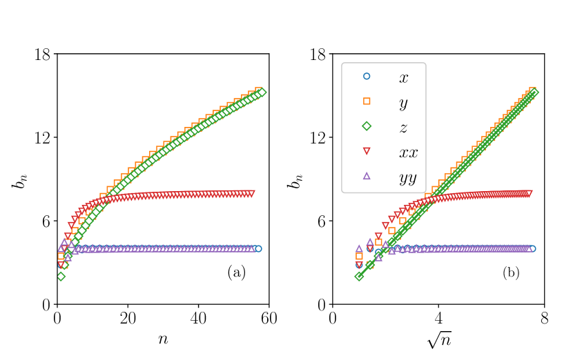
Figure 1: Plots of $b_{n}$ for the t-Ising model ($h=1$ and $g_{l}=0$) with respect to $n$ in (a) and $\sqrt{n}$ in (b). $b_{n}$ of $O^{z}$ is in perfect agreement with the straight line in (b).

The scaling behavior of the Lanczos coefficient is consistent with the time dependence of the autocorrelation functions. Brandt and Jacoby [42] derived that $C_{x}(t)\equiv\langle\sigma_{0}^{x}(t)\sigma_{0}^{x}(t)\rangle=J_{0}(4t)^{2}+J_{1}(4t)^{2}\simeq\frac{1}{2\pi t}\left(1-\frac{\cos 8t}{8t}\right)$. It decays algebraically with an oscillating component, which is a characteristic of the operators of type I. They also derived that $C_{z}(t)\equiv\langle\sigma_{0}^{z}(t)\sigma_{0}^{z}(0)\rangle=e^{-2t^{2}}$, which shows that $O^{z}$ is an operator of type II with $\alpha=2$. The Lanczos coefficient for $O^{y}$ also scales as $b_{n}\sim\sqrt{n}$ with an alternating finite-$n$ correction. The correction term indicates a power-law correction to the Gaussian autocorrelation function [32].

We also studied the t-Ising model with $h\neq 1$. We found that finite-$n$ corrections become larger, but the qualitative behavior does not change. Summarizing the results, the Lanczos coefficients in the integrable t-Ising model are of type I or II, depending on the choice of observables.

IV.2 tl-Ising model with uniform longitudinal field

The longitudinal field breaks the integrability of the t-Ising model [22]. It is accepted that an integrable system becomes quantum chaotic immediately as a uniform integrability breaking field turns on. Various studies on energy-level spacing statistics [43, 44, 45, 46] and on the eigenstate thermalization hypothesis [44, 47] confirm that a nonzero integrability breaking field results in quantum chaos. Furthermore, the fidelity susceptibility measurement suggests that the threshold value of an integrability breaking field necessary for the onset of quantum chaos vanishes in the thermodynamic limit [48, 49]. We will investigate the transition to the quantum chaos by the uniform longitudinal field in the context of the operator growth.

It is conjectured that the operators of the one-dimensional chaotic systems should follow the scaling law $b_{n}\propto n/W(n)$ with the Lambert $W$ function $W(n)\simeq\ln n$ [17]. Numerical data for the tl-Ising model in Ref. [17] seem to be consistent with the conjecture. However, the logarithmic corrections are not clearly visible in the data up to $n\lesssim 30$. In this subsection, we establish the scaling form $b_{n}\sim n/W(n)$ when the uniform longitudinal field $g_{l}=g$ is strong. We also investigate the crossover when $g$ is small.

We first report the results for the observable $O^{x}$ that exhibits the scaling behavior of type I in the t-Ising model. Numerical data are presented in Fig. 2. The Lanczos coefficient increases with $n$ for $g\neq 0$. However, there is an overall downward curvature suggesting that the growth is sublinear. It turns out that the logarithmic correction is responsible for the curvature. In Fig. 2(b), we plot $n/b_{n}$ as a function of $W(n)$. When $g=1$, the data are in excellent agreement with a straight line. It confirms the proposed scaling $b_{n}\propto n/W(n)$ for the one-dimensional quantum chaotic systems.

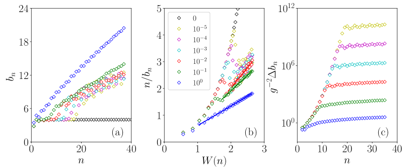
Figure 2: Lanczos coefficients for the operator $O^{x}=\sigma_{0}^{x}$ in the tl-Ising model with $h=1$. (a) The Lanczos coefficients at several values of the uniform longitudinal fields $g$ are compared. (b) Plots of $n/b_{n}$ against $W(n)$. Data for $n>n_{c}(g)$ are in agreement with the straight lines, which indicates that $b_{n}\propto n/W(n)$ for $n>n_{c}(g)$. (c) Scaling plot of $g^{-2}\Delta b_{n}$ vs $n$.

When the longitudinal field $g$ is weak, we find an interesting crossover at $n=n_{c}(g)$. The operator spreads as in the integrable system ($b_{n}(g)\simeq b_{n}(g=0)$) for small $n\ll n_{c}(g)$, then as in the chaotic system ($b_{n}\sim n/W(n)$) for $n\gg n_{c}(g)$. We have performed a quantitative analysis and found that

$$\Delta b_{n}\equiv\frac{b_{n}(g)-b_{n}(0)}{b_{n}(0)}\propto g^{2}$$ (9)

for $n\ll n_{c}(g)$. Figure 2(c) presents the plot of the scaled difference at several values of $g$. The scaling plot demonstrates that the scaled differences $g^{-2}\Delta b_{n}$ from different values of $g$ lie on a single curve, represented by a scaling function $\mathcal{F}_{x}(n)$, until they cross over to the asymptotic behavior at $n\simeq n_{c}(g)$ [see Eq. (12)]. Figure 2(c) indicates that the scaling function has an exponential shape $\mathcal{F}_{x}(n)\sim e^{an}$ for large $n$ so that the crossover depth $n_{c}(g)$ scales as

$$n_{c}(g)\sim|\ln g|.$$ (10)

The logarithmic dependence can be also inferred from the plots in Figs. 2(a) and 2(c), where the crossover points $n_{c}(g)$ are shifted by a constant amount per tenfold increase of $g$.

The crossover has an implication on the operator growth dynamics in the Krylov space. At short times until $(n)_{t}$ reaches $n_{c}$, the operator spreads as in the integrable systems. Since the mean depth grows as $(n)_{t}\sim t$ in the type-I dynamics, the system reaches the crossover depth $n_{c}(g)$ at the crossover time $t_{c}$

$$t_{c}(g)\sim n_{c}(g)\sim|\ln g|.$$ (11)

Afterward, the generic spreading dynamics of the nonintegrable systems sets in.

The crossover explains the mechanism for the transition from prethermalization to thermalization. When an integrable system is perturbed by an integrability breaking field, an observable temporarily remains at a nonthermal value predicted by the generalized Gibbs ensemble, and then tends to the thermal equilibrium value in the long time limit [23, 24, 25, 26, 27, 28, 29]. The thermalization dynamics is characterized by the rate which is proportional to the integrability breaking field strength squared [26, 25]. The thermalization rate is manifest in the quadratic scaling in Eq. (9). Besides the thermalization rate, to the best of our knowledge, the crossover time following the scaling law of Eq. (11) has not been reported yet.

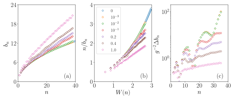
Figure 3: The same plots as in Fig. 2 for the operator $O^{z}=\sigma_{0}^{z}$.

We also report the results for the operator $O^{z}=\sigma_{0}^{z}$ in Fig. 3. The operator exhibits the scaling behavior of type II in the integrable t-Ising model. Figures 3(a) and 3(b) confirm that the Lanczos coefficient scales as $b_{n}\sim n/W(n)$ when the integrability breaking field $g$ is large enough. The crossover also occurs for small $g$. It is less trivial to locate the crossover depth $n_{c}(g)$ from the numerical data in Figs. 3(a) and 3(b). Nevertheless, we find that the scaling law in Eq. (9) is also valid for the operator $O^{z}$, which is confirmed with the scaling plot in Fig. 3(c). The scaling implies that the thermalization rate is also given by $\sim g^{2}$. Note that the scaling function for $O^{z}$ has a complicated shape with oscillatory behavior, which makes it difficult to locate the crossover depth $n_{c}(g)$.

IV.3 tl-Ising model with a longitudinal field at a single site

Integrability can be broken with a local perturbation [50, 51, 48, 52]. For the integrable XXZ spin chain perturbed with a local magnetic field applied to a single site, the fidelity susceptibility measurement reveals that the system becomes chaotic at any nonzero value of the magnetic field in the thermodynamic limit [48]. The t-Ising model has been also studied with a local longitudinal field applied to a single site [52].

In the perspective of the operator growth, it is surprising that the local perturbation leads to the quantum chaos. The operator growth in the Krylov space is accompanied with the spatial growth of the operator support. With local perturbation, the support is affected minimally by a local perturbation. We investigate the impact of the local perturbation on the operator growth dynamics in the tl-Ising model with the Hamiltonian in Eq. (8) with $h=1$ and $g_{l}=g\delta_{l0}$.

Figure 4 presents the Lanczos coefficient for the operator $O^{x}=\sigma_{0}^{x}$ when the local field strength $g\leq 10^{-1}$ is weak. The operator $O^{x}$ follows the growth dynamics of type I without the longitudinal field. Figure 4(a) looks similar to Fig. 2(a). The system undergoes a similar crossover at the depth $n=n_{c}(g)\propto|\ln g|$. On the other hand, $b_{n}(g)$ for $n>n_{c}(g)$ shows a more pronounced downward curvature than in Fig. 2. To characterize the asymptotic scaling behavior of $b_{n}$, we plot the Lanczos coefficient with respect to $\sqrt{n}$ in Fig. 4(b). The data for large $n$ are well fitted to a straight line, which implies that $b_{n}\sim\sqrt{n}$, characteristic behavior of type-II dynamics. The asymptotic behavior, however, is not consistent with the quantum chaotic scaling $b_{n}\sim n/W(n)$. In Fig. 4(c), we present the plots of $n/b_{n}$ against the Lambert W function $W(n)$. The convex curvature invalidates the scaling form $b_{n}\sim n/W(n)$. Thus, we conclude that the weak local perturbation is not sufficient to lead to the quantum chaos. It only modifies the the operator growth dynamics from type I to type II.

Figure 4: Lanczos coefficients for the operator $\sigma_{0}^{x}$ in the tl-Ising model with $h=1$ and $g_{l}=g\delta_{l0}$ with $g\leq 0.1$. (a) The Lanczos coefficients at several values of the local longitudinal fields $g$ are compared. There is a crossover from the type-I behavior. (b) Plots of $b_{n}$ against $\sqrt{n}$. The straight line represents a linear fit of the data with $g=0.1$ for $n\geq 13$. (c) Plots of $n/b_{n}$ against $W(n)$. The straight line also represents a linear fit of the data with $g=0.1$.

We also investigate the scaling behavior of $b_{n}$ when the local field strength is large. As $g$ increases, an oscillatory behavior sets in, which obscures the asymptotic scaling behavior (see Fig. 5). The oscillatory behavior is reminiscent of the one observed in Fig. 3. We speculate that the oscillatory behavior is a signature to a transition from the scaling of type II to the quantum chaotic scaling. However, a decisive conclusion cannot be drawn from the numerical data.

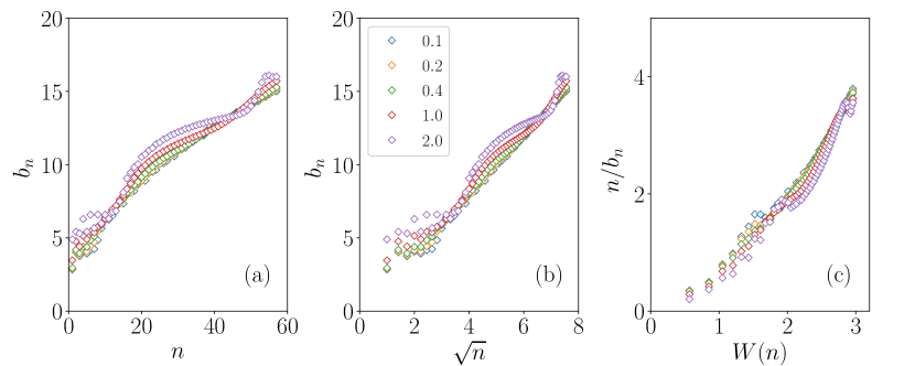
Figure 5: Lanczos coefficients for the operator $\sigma_{0}^{x}$ in the tl-Ising model with $h=1$ and $g_{l}=g\delta_{l0}$ with $g\geq 0.1$. The data are plotted in the same way as in Fig. 4.

We conclude that the weak local longitudinal field applied to the t-Ising chain does not give rise to the quantum chaos: The threshold $g_{c}$ of the quantum chaos transition, if any, should be nonzero. It is in contrast to the XXZ spin chain which undergoes an immediate transition to the quantum chaos [48].

V Summary and Discussions

We have investigated the operator growth dynamics in the one-dimensional transverse-field Ising model perturbed with the uniform and local longitudinal field. Without longitudinal field, the Lanczos coefficient $b_{n}$ converges to a constant (type I) or scales as $O(\sqrt{n})$ (type II) depending on the choice of local operators. When the longitudinal field is uniform and strong enough, the Lanczos coefficient grows as $O(n/\ln n)$, which corresponds to the the maximum growth for a one-dimensional system with local interactions. Our extensive numerical data in Figs. 2 and 3 confirm the existence of the logarithmic correction to the linear scaling. We were able to detect the logarithmic correction with the help of the scaling analysis on the numerical data $b_{n}$ for large values of $n$. These results support the hypothesis of Ref. [17] that the operator growth dynamics is a universal indicator of quantum chaos.

We have also discovered that the operator growth dynamics exhibits a crossover scaling as the system undergoes a transition from an integrable nonergodic state to a nonintegrable quantum chaotic state. When the uniform longitudinal field strength $g$ is small, the Lanczos coefficients $b_{n}$ for $n\ll n_{c}(g)$ follow the scaling form

$$\frac{b_{n}(g)-b_{n}(0)}{b_{n}(0)}=g^{2}\mathcal{F}_{O}(n)$$ (12)

with an operator-dependent scaling function $\mathcal{F}_{O}$ [see Figs. 2(c) and  3(c)]. For $n\gg n_{c}(g)$, $b_{n}$ crosses over to the scaling form $O(n/\ln n)$. The crossover scaling is the irrefutable evidence that the integrability breaking transition occurs $g_{c}=0$. The crossover scaling form is related to the prethermalization dynamics. Since the Lanczos coefficient has the dimension of the inverse time, the scaling factor $g^{2}$ corresponds to the thermalization rate. The crossover depth scales as $n_{c}(g)\sim|\ln g|$ for the operator $\sigma_{0}^{x}$. The implication of the crossover depth on the thermalization dynamics has to be studied further. The crossover scaling analysis also reveals that a local longitudinal field at a single site does not give rise to the quantum chaos immediately.

In conclusion, we establish that the operator growth dynamics faithfully reflects the quantum chaos in the transverse field Ising spin chain. Furthermore, we show that it is a useful tool to characterize the transition of the integrable system to the quantum chaos induced by the integrability breaking field.