∎
Corresponding Author E-mail: garne214@umn.edu 33institutetext: 2. Department of Industrial and Systems Engineering, University of Minnesota 44institutetext: Union Street SE, Minneapolis, MN, 55414, USA
44email: zhangs@umn.edu
Linearly-Convergent FISTA Variant for Composite Optimization with Duality
Abstract
Many large-scale optimization problems can be expressed as composite optimization models. Accelerated first-order methods such as the fast iterative shrinkage-thresholding algorithm (FISTA) have proven effective for numerous large composite models. In this paper, we present a new variation of FISTA, to be called C-FISTA, which obtains global linear convergence for a broader class of composite models than many of the latest FISTA variants. We demonstrate the versatility and effectiveness of C-FISTA through multiple numerical experiments on group Lasso, group logistic regression and geometric programming models. Furthermore, we utilize Fenchel duality to show C-FISTA can solve the dual of a finite sum convex optimization model.
Keywords:
composite optimization accelerated first-order algorithm Fenchel duality group LassoMSC:
90C25 65K10 49M29 90C061 Introduction
The following composite optimization model,
| (1) |
where is a closed, convex subset of , is a smooth, convex function, is convex but potentially non-smooth, is a smooth mapping, and is a convex function over , has received ample attention in the literature BT09 ; BF95 ; DDL18 ; DDP19 ; N13 ; W90 . A special case of (1) of immense importance is the additive composite optimization model,
| (2) |
which envelopes a plethora of models including: compressive sensing CP16 , Lasso T96 , and group Lasso and group logistic regression models QSG13 ; YLY11 as well as several machine learning constructs such as support vector machines. Due to their dimensionality, many large-scale optimization models have rendered second-order methods computationally impractical; thus, efficient and accelerated first-order algorithms have become essential for tackling numerous problems. With the advent of Nesterov’s seminal work N83 much effort has been expended toward the development of accelerated first-order methods. For a comprehensive overview of this line of research see the monograph of d’Aspremont et al. and the references therein AST21 . As an example, utilizing Nesterov acceleration, Beck and Teboulle developed the influential fast iterative shrinkage-thresholding algorithm (FISTA) BT09 which obtained the optimal sublinear convergence rate for (2) with and convex and possibly non smooth. In recent years, under the assumption and potentially are strongly convex, many accelerated versions of FISTA for (2) have been developed which obtain the optimal linear convergence rate proved by Nesterov CC19 ; CP16 ; FV19 ; FV20 ; RC21 .
Furthermore, recent work has been done to determine conditions which lighten the assumption of strong convexity while maintaining accelerated and at times linear convergence BS17 ; DDL18 ; ING19 . In DDL18 the authors demonstrate local linear convergence to a first-order stationary point for (1) without assuming any strong convexity on . The authors extended the work in ZZ17 by utilizing a specific error bound condition (Definition 3.1 in DDL18 ) in tandem with an assumption on the quadratic growth of the objective function.
In this paper we develop an accelerated composite version of FISTA, C-FISTA, similar to the recent FISTA variants which extends to solving model (1) as well as model (2). Also, in line with the recent works DDL18 ; DDP19 , we forgo any assumption guaranteeing strong convexity of the objective function in (1) and prove C-FISTA obtains global linear convergence under certain error bound conditions.
1.1 Main Contributions
This paper presents three main contributions. The first contribution of this paper is the development of an accelerated version of FISTA which obtains global linear convergence for (1) under specific assumptions. Our algorithm, C-FISTA, differs from the aforementioned FISTA variants because they were either exclusively designed for the additive composite model (2) or only obtained local instead of global linear convergence for the more generalized model (1). We demonstrate that C-FISTA is a generalization of the FISTA variant GFISTA CC19 ; CP16 when proving C-FISTA is an extension of recent algorithmic developments. Further, we present an alternative convergence analysis than those presented for the other accelerated FISTA variants and exclude any reference to the strong convexity parameter of as done in CC19 ; FV19 ; FV20 .
The second contribution of this paper is our utilization of Fenchel duality to develop dual models which can be solved via C-FISTA, and our leveraging of Fenchel duality theory HL88 ; RF70 ; Roos20 to enable efficient computation of the subproblems of C-FISTA. Additionally, we outline a dual algorithmic approach for a general convex model which can be solved by C-FISTA and generalizes the approaches of Han and Lou HL88 and Auslender A92 among others FHN96 ; GM89 . Sections 4 and 5 provide the relevant background on Fenchel duality and provide an example on how we utilize the theory in the implementation of C-FISTA.
The third contribution of this paper is the presentation of globally linearly convergent algorithms for solving various Lasso and logistic regression models with C-FISTA. In our numerical experiments, we demonstrate C-FISTA outperforms FISTA BT09 and the SLEP software package SLEP for solving group, sparse-group and overlapping sparse-group Lasso models and sparse-group logistic regression models. We also compare C-FISTA with ADMM on the Lasso models, which has proven linear convergence for various Lasso formulations HQL17 , and demonstrate superior convergence after tuning ADMM in our numerical experiments. Lastly, we demonstrate C-FISTA’s applicability for solving a class of geometric programming models.
1.2 Organization of the Paper
In Section 2 we present C-FISTA and prove the global linear convergence of the algorithm under certain assumptions. Section 3 motivates C-FISTA by describing the Lasso, logistic regression and geometric programming models which are solvable with C-FISTA. In Section 4 we present the necessary background on Fenchel duality and make connections to our accelerated FISTA algorithm, and Section 5 provides an example of how Fenchel duality informs our application of C-FISTA to solve the crucial proximal mapping step. Section 6 contains the algorithms for solving the Lasso, sparse-group logistic regression and geometric programming models with C-FISTA, and our numerical experiments comparing C-FISTA to other efficient first-order algorithms. The paper concludes in Section 7 with some final remarks and potential avenues for future investigation.
2 A Generalized Composite Optimization Algorithm
In this paper, our primary focus revolves around the composite optimization model,
where is a closed, convex subset of , is a smooth, convex function, is convex but potentially non-smooth, is smooth and defined as with Jacobian, , at . For convenience in our analysis we denote . A key assumption for feasible implementation is that the following proximal mapping with respect to is efficiently computable:
where . We now state the four main assumptions in our analysis:
-
(A0)
is strongly convex with parameter and gradient Lipschitz with parameter , and is convex over .
-
(A1)
is Lipschitz continuous with parameter , and has Lipschitz gradient constant for .
-
(A2)
There exists such that for all .
-
(A3)
There exists such that with ,
Our analysis focuses on the proposed algorithm C-FISTA (Algorithm 1). However, before stating the algorithm and proving our convergence results, we further frame the assumptions.
2.1 Discussion of Assumptions
In this section we further detail the assumptions and demonstrate how they compare to standard assumptions in the literature. Before expounding upon (A0) - (A3), we first make the essential observation that under these assumptions it is possible is not strongly convex in . Letting , we do see, however, that the descent inequality and the strongly convex inequality still hold for with respect to and , i.e. for all ,
where and
For the remainder of the paper, we will reserve to denote , that is .
Of the assumptions, (A0) and (A1), are the most straightforward. The first assumption is standard in the literature, and the second ensures is sufficiently well-behaved in terms of its continuity and differentiability; however, no convexity assumptions are made directly on the component functions .
Remark 1
From assumption (A1) we obtain a few important inequalities. First, utilizing the fact each is Lipschitz continuous, it follows from the limit definition of the directional derivative that for all . Therefore, letting be fixed we see that,
So, defining,
| (6) |
we have,
| (7) |
In regards to (A2), we note it is a condition which depends as much on the constraint set as it does on the function . For example, if with singular, then (A2) will fail to hold if ; however, it will be satisfied if . Additionally, this condition is fundamentally different than growth conditions about the set of optimal solutions such as given in DDL18 because it places no condition on the proximal mapping nor relates to the set of optimal solutions of (1).
Assumption (A3) by all appearances is the most opaque; however, (A3) is essentially equivalent to assuming is gradient Lipschitz continuous. If it is assumed is gradient Lipschitz with parameter , then (A3) follows with . Similarly, if assumption (A3) holds, then is gradient Lipschitz with parameter . Therefore, this assumption is fundamentally a constraint on the gradient of which is unlike standard error bound or growth conditions found in the literature.
As a closing remark on the assumptions, which we will revisit following the proof of Theorem 2.1, although (A2) and (A3) are stated in a global fashion they only need to hold near the iterates generated by Algorithm 1. For the sake of our argument, we require our assumptions to hold on ; however, in practice this is unnecessary and we demonstrate this through several numerical experiments in Section 6.
2.1.1 Example Models
Before beginning our analysis of Algorithm 1 it makes sense to introduce a few models which will appear frequently in the applications presented in the forthcoming sections, and provide an exposition on their relationship to the stated assumptions.
-
•
If is affine linear, i.e. for and , then (A1) is met and the convexity of follows readily without the need for any additional assumptions on . Furthermore, (A3) is trivially satisfied with since . As previously stated, (A2) will hold provided . Finally, from (6) we see in (8) can by given as the largest eigenvalue of . Thus, in this setting, we always have and .
-
•
In the geometric programming model discussed in Section 6.5, we have with a closed, bounded, convex subset of the positive orthant in . Thus, (A1) holds and, as will be shown in Section 6.5, constants and can be computed which satisfy the necessary inequalities over the constraint set. This example is significant because it demonstrates non-linear and non-convex choices for are admissible for certain models.
2.2 C-FISTA Convergence Analysis
We now state the formal description of the C-FISTA algorithm, and present the main convergence result which provides a global linear convergence guarantee.
Theorem 2.1
Assuming assumptions (A1) - (A3) hold with and convex, then C-FISTA has an accelerated global linear rate of convergence for (1); that is, for each iteration, we have,
| (9) |
In particular, if we perform C-FISTA for iterations, then it holds that,
| (10) |
Proof
By the Lipschitz inequality for ,
where the second line follows from (8) and the last lines are a result of the Newton-Leibniz formula. Applying assumption (A3) we obtain,
Utilizing the strong convexity of , for all we have,
where the second inequality follows from (A2). Applying (A3) and utilizing a similar argument with the Newton-Leibniz formula it follows,
| (11) | |||||
By the first order optimality conditions of (3) we have,
where is an element of the subgradient of at . The optimality conditions above along with the convexity of and (11) give us,
| (12) | |||||
Let , whose exact value is to be determined later. Take in (12) and multiply by on both sides of the expression. Then, let in (12) and multiply by on both sides. Finally, adding up these two resultant inequalities and applying the assumption we have,
| (13) | |||||
Recall from (5) that,
where the value of the parameter will be determined later. Thus,
| (14) | |||||
Take , whose value will be determined in a moment. Multiplying by on both sides of (14), and adding the resulting inequality to (13) we obtain,
if we choose the parameters to take the values
| (15) |
Observe . Since , and , it follows
Note in the last step above, we used (3),
Therefore, , and so
Hence, we have for all ,
| (16) |
and so by induction starting from the -th iteration we obtain the result. ∎
Remark 2
If we have , then assumptions (A1) - (A3) hold trivially. Also, we have , and ensuring which gives us the convergence result,
If , then this is the same convergence result produced by GFISTA CC19 ; CP16 which is an accelerated variant of FISTA for (2). Therefore, C-FISTA generalizes GFISTA into the broader problem class given by the composite optimization model (1).
Remark 3
The condition essentially requires that the product of the first-order derivatives of and the second-order derivative of should not exceed the product of their curvatures. In some cases, this condition is easy to satisfy by variable-transformation, or scaling. For example, when is homogeneous of degree , i.e. for any and , and is homogeneous with degree , i.e. . Then for any one can scale the variable as , and the problem is turned equivalently into minimizing . After the above change of variables, the new objective has the modified parameters , , and . Therefore, in this situation by appropriately choosing one can always satisfy the condition .
As mentioned previously in Section 2.1, the global nature of assumptions (A2) and (A3) are in many instances stronger than necessary. From the proof of Theorem 2.1, we see these assumptions only need to hold locally about the and sequences generated by C-FISTA. Enforcing the conditions to hold on the span of the constraint set ensures global linear convergence; however, even when the assumptions are not strictly satisfied on the span, C-FISTA still proves to be effective in practice. In Section 6, we will demonstrate the effectiveness of C-FISTA on group Lasso and geometric programming models where the assumptions are not strictly met globally but asymptotic linear convergence is still achieved. Ultimately, the success of C-FISTA in these regimes demonstrates the current gap between theory and practice; further research should shrink this separation and provide a direction for future inquiry.
3 Motivation: Lasso, Logistic Regression & Geometric Programming
A class of motivating composite optimization models for which C-FISTA is applicable are the various Lasso formulations. The standard Lasso model originating from Tibshirani T96 ,
is solvable via C-FISTA. All the assumptions for Algorithm 1 will be satisfied when is of full-column rank, but, as we will see in Section 6.2.2, C-FISTA demonstrates linear convergence when is not of full-rank and the assumptions are almost but not completely met. The results from Section 2 further guarantee global linear convergence to the optimal solution even when there exists a constraint on . For example, Algorithm 1 can solve the following constrained Lasso model,
The utility of the Lasso model is detailed extensively in the literature; see JOV9 ; QSG13 ; YLY11 ; YL7 ; ZZST20 . The success of the basic model spawned the development of several Lasso variants including: the group Lasso (GL) model QSG13 ; YL7 ,
where is a subvector of corresponding to the indices in where disjointly partitions , the sparse-group Lasso (SGL) model SFHT13 ; ZZST20 ,
and the overlapping group and overlapping sparse-group Lasso (OSGL) models JOV9 ; YLY11 ; ZZST20 which are of identical form to the group Lasso and sparse-group Lasso models respectively, expect no longer is a disjoint partition of . As we will see in Section 5, the subproblems required in C-FISTA for the Lasso models are solvable in closed form or by an efficient subroutine in the case of the overlapping group/sparse-group Lasso models with global linear convergence achieved in each variant.
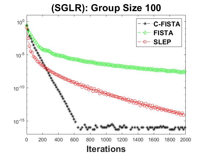
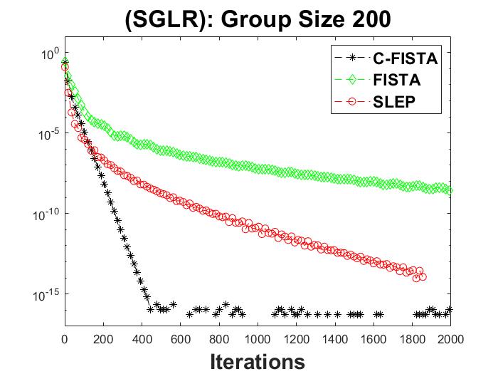
Another model where C-FISTA has demonstrated linear convergence is the sparse-group logistic regression (SGLR) model SLEP ; MGB8 ,
where is a vector containing only entries of . The sparse-group logistic regression model has applications in various machine learning models especially in the area of classification, and the subproblems for the logistic regression model are in the same format as the sparse-group Lasso model detailed extensively in Section 5.
A final motivating model is geometric programming. Geometric programming is a useful modeling paradigm which has numerous applications especially in electrical circuit design. A full description and tutorial on these models is provided by Boyd et al. in GP . A regularized subclass of geometric programs solvable via C-FISTA is,
where , for all , and is a closed and bounded convex subset of . The condition ensures the model is convex. In solving this model, we decompose the objective such that . Allowing non-linear and non-convex component functions for demonstrates the novelty of C-FISTA to escape strictly affine compositions showcasing a level of extended generality.
Before discussing how to compute subproblems for the Lasso models, we first discuss Fenchel duality in Section 4 and describe how C-FISTA can be utilized via a dual approach to solve a general constrained composite model.
4 A Dual Formulation and Algorithmic Approach
In this section, we outline the construction of a dual algorithm using Fenchel duality which generates an approximate primal solution from the dual solution at every iterate. To elucidate this approach we first provide a brief overview of standard convex analysis results regarding conjugate functions and Fenchel duality RF70 ; Roos20 . Unless otherwise stated, we use the standard notation of Rockafellar RF70 . For generality, we will consider the following constrained composite model:
| s.t. |
where the ’s are proper convex functions on and the ’s are closed convex subsets of . To begin, let us introduce some basic notions in convex analysis.
Let be a closed convex set. The support function of is defined as,
and the polar set of is,
Thus, we can succinctly write, . Let be a convex function whose domain is contained in . The conjugate of is defined as,
where the function is assumed to take value anywhere outside its domain. In deriving the Fenchel dual of (4) we need some standard results from convex analysis.
Lemma 1
Suppose is a proper convex function, then
| (18) |
Lemma 2
(Theorem 16.4 RF70 ) Suppose are proper convex functions on and the intersection of the relative interiors of the domains of the ’s is non-empty, then
| (19) |
Lemma 3
For a convex set , suppose its indicator function is defined as,
Then, the conjugate of the indicator function is simply the support function of ;
The proofs of Lemmas 1 and 3 follow directly from the definitions of conjugate and support functions. Thus, rewriting (4) in the equivalent form,
| s.t. |
and utilizing Lemmas 1, 2, and 3, the Fenchel dual of (4) is:
| s.t. |
Note, for the sake of presentation we have written the dual problem (4) in such a manner that the optimal solutions of (4) and (4) differ by a negative sign. To better understand the link between the primal and dual models, we demonstrate how the optimality conditions of (4) and (4) are linked. Assuming the conjugate functions of the ’s () are differentiable and denoting for to be optimal for (4), we have the first-order optimality conditions,
| (21) |
Denoting , the optimality conditions imply for , and so by Lemma 5 of Z18 , , for . Similarly, because , if , then , which means that is a normal direction at :
Furthermore, by (21)
| (22) |
Thus, the first-order optimality conditions for the dual problem implies (22), which is the optimality condition for the primal problem (4). To see this, note that
and so,
We now present an important relationship between the primal solution induced by the dual iterations which outlines a dual approach to solving (4).
Proposition 1
Suppose that is a strongly convex function with strong convexity parameter and gradient Lipschitz constant . Let be a sequence converging to the dual solution . For each in the dual sequence, we recover a primal solution such that,
Proof
By the Fenchel duality relation, we know that is also a strongly convex function with strong convexity parameter and gradient Lipschitz constant (Theorem 1 Z18 ). Further, by the definition of and previously stated results, . Therefore, , and so the gradient Lipschitz condition on yields,
On the other hand, the gradient Lipschitz condition on states,
∎
Therefore, the above result gives us the framework to develop a general dual approach to solving (4). Applying any algorithm to solve the dual problem (4) we can recover a primal solution at each iteration; furthermore, the rate of convergence on the primal side for any algorithm will only differ by a fixed constant, , in-comparison to the rate of convergence on the dual side.
The presented dual formulation is not novel; Han and Lou HL88 and Fukushima et al. FHN96 have very similar derivations of the dual and many algorithms such as Dykstra’s projection algorithm GM89 utilize Fenchel duality. The clarity provided by the previous result is that, under the assumption is strongly convex with gradient Lipschitz, any algorithm which generates a converging dual solution will generate a primal solution with the same rate of convergence up to a constant factor. This is directly relevant to our proposed algorithm because the dual (4) is solvable via C-FISTA. Let , and such that,
where is the identity matrix and is the block matrix with the identity matrix in the k-th position, e.g. , then we can rewrite (4) as,
With this decomposition it is straightforward to specify the constants: , , , and for C-FISTA. Assuming is strongly convex with parameter and gradient Lipschitz with constant , it follows and . The linearity of yields , and the simple structure of the mapping gives . Lastly, since the matrix defining is singular; however, though does not strictly satisfy assumption (A2), in practice C-FISTA will often converge for a range of small values. This is demonstrated in Section 6.2.2 through multiple numerical experiments on an underdetermined group Lasso model and follows from our previous discussion on the overly strict nature of the assumptions which ensure global linear convergence.
A final note must be made in-regards to the proximal mapping step which would be required to solve the dual formulation. Computing in this case would depend on the definitions of and . This could prove difficult; however, presents a natural decomposition such that only the individual proximal mappings of the functions and would be necessary. This substantially simplifies the procedure enabling tractable computations in many instances.
Therefore, we see that (4) under the proper convexity assumptions has a dual which in many cases is solvable via C-FISTA, and Proposition 1 demonstrates the primal solution is recoverable from the dual solution without losing linear convergence.
Besides using Fenchel duality to directly solve the dual model with C-FISTA and recover the primal solution, we can also utilize Fenchel duality theory to solve the intermediate subproblems in the primal implementation of C-FISTA. In the next section, we describe this process using the sparse-group Lasso model as an example.
5 Solving Subproblems with Fenchel Duality
One example of how duality can be leveraged to apply C-FISTA can be seen in how we solve the subproblems for the group and sparse-group Lasso models. In the sparse-group Lasso model, the main subproblem which needs to be solved to apply C-FISTA is of the form,
with . Utilizing Lemmas 1 and 2 and standard conjugate functions Roos20 , we see the Fenchel dual of is,
When is fixed, consider the simple projection problem,
whose solution is explicit:
Therefore,
Thus, the dual problem is equivalent to , which can be solved through the associated model,
Since the individual components of are decoupled in , the above problem can be reduced to solving 1-dimensional problems,
for . Observe that the solutions for the above 1-dimensional models can be found using the following thresholding operator:
Therefore, a solution for is , where for all , and,
After solving with the optimal solution , one recovers the optimal solution to as using the results from Section 4. In particular,
Hence, by Fenchel duality we obtain a closed form solution to yielding an exact solution to the required subproblems to apply C-FISTA to the sparse-group Lasso model. Similar approaches can be taken to solve other potential subproblems which arise when applying C-FISTA. In the next section, we present the algorithms and numerical experiments for solving the models discussed in Section 3.
6 Numerical Experiments
To demonstrate the practicality and efficiency of C-FISTA, we conducted numerous experimental tests on group Lasso, sparse-group Lasso, overlapping sparse-group Lasso, sparse-group logistic regression, and regularized geometric programming models. The overall structure of this section is as follows: Subsection 6.1 details how to apply C-FISTA to solve the Lasso formulations; Subsection 6.2 contains the results of the numerical experiments conducted on the Lasso models; Subsections 6.3 and 6.4 present the solution procedure and numerical results for the sparse-group logistic regression model; Subsections 6.5 and 6.6 describe the application of C-FISTA to a set of regularized geometric programs and presents some numerical results.
6.1 Lasso Models
In this section we state how to apply C-FISTA to solve the various Lasso models described in Section 3. In order to apply C-FISTA, the practitioner must select a decomposition of the objective function, i.e. the user must define and in (1). For the sake of exposition, in Sections 6.1.1, 6.1.2, and 6.1.3, we decompose as and . By doing this we have , , and . Therefore, the strong convexity constant and gradient Lipschitz constant for are the only parameters which must be estimated to apply C-FISTA. This was the convention chosen for the algorithms presented in these sections as it enables more concise algorithmic descriptions; however, another viable decomposition is to have and . This decomposition is utilized in Section 6.2.2. Under this decomposition, one readily obtains the strong convexity and gradient Lipschitz constants as . As for the other constants, the linearity of yields and . Hence, the only constant to estimate is from assumption (A2). The ability to chose the decomposition for a particular problem is a benefit of C-FISTA. This freedom enables the practitioner to select the most beneficial and/or convenient decomposition for their model of interest.
We now begin our discussion with how to apply C-FISTA to the group Lasso formulation.
6.1.1 C-FISTA for Group Lasso
Applying C-FISTA to solve any model hinges on computing the proximal mapping in (3). This key subproblem in the group Lasso model is of the form,
| (23) |
which by the first-order optimality conditions has the simple closed-form solution,
With the solution to the group Lasso subproblems (23), we write down how to solve the group Lasso model with C-FISTA in Algorithm 2 where and .
Practical application of Algorithm 2 requires the user to determine bounds for the Lipschitz constant and strong convexity constant of . For the group Lasso models making such bounds readily available. By the definition of strong convexity we see . Similarly, using the definition of the Lipschitz constant, we see that where and are the smallest and largest eigenvalues of respectively. For other strongly convex functions on which C-FISTA is applicable, tight bounds for and might be unavailable. In these situations conservative estimates for these bounds or a backtracking scheme such as in BT09 to estimate these parameters would be required. In this paper we do not focus on subroutines to estimate these bounds in our algorithms; however, the backtracking strategies applied in BT09 ; CC19 ; FV19 could similarly be implemented in many instances of C-FISTA.
6.1.2 C-FISTA for Sparse-Group Lasso
The key subproblem in applying C-FISTA to solve the sparse-group Lasso model was determined in Section 5; thus, we can write Algorithm 3 to solve the sparse-group Lasso model with C-FISTA.
Since is identical in all of the Lasso models, the same bounds for the Lipschitz and strong convexity constants in Algorithm 2 apply for each of the Lasso models. Comparing Algorithms 2 and 3, we note only Step 2 has been updated because the and -updates are independent of the objective function. The alteration in Step 2 is solely due to the difference in the regularization term in the group and sparse-group Lasso models which alters the proximal mapping (3).
6.1.3 C-FISTA for Overlapping Sparse-Group Lasso
The key difference between the overlapping sparse-group Lasso model and those previously discussed is the removal of the prohibition that the groups of variables cannot intersect. Allowing overlapping groups of variables removes the ability to decouple the minimization in (3) into subproblems over the individual subvectors. In the sparse-group Lasso model, since the groups of variables do not overlap, we were able to show in Section 5 there was a closed form solution to the proximal mappings; however, with overlapping groups the key subproblem for implementing C-FISTA,
| (24) |
is no longer decomposable and a simple closed form solution is unobtainable; therefore, we must solve this subproblem numerically at each iteration in-order to apply C-FISTA to the overlapping sparse-group Lasso model. In YLY11 the authors apply a variation of FISTA to solve the (OSGL) model. Our approach is distinct from their approach because we accelerate FISTA through the use of two sequences, and , while they use a single sequence performing a Nesterov-like acceleration. In order to apply their algorithm, the authors of YLY11 developed an efficient subroutine, overlapping.c, to numerically solve (24). Their subroutine is provided in the SLEP software package SLEP . In our solving of the (OSGL) model with C-FISTA, we apply Algorithm 3 exactly in the same fashion as for the sparse-group Lasso model except when computing in Step 2 we solve (24) with overlapping.c from the SLEP software package.
6.2 Lasso Numerical Experiments
In this section, we describe the results from the numerical experiments conducted on the Lasso models. In the first set of experiments, the data matrix has full-column rank. In this setting, all assumptions stated in Section 2 are fully met. In practice, however, it is often unrealistic to assume the data matrix for a Lasso model is overdetermined; therefore, we conducted a second set of experiments on the group Lasso model with underdetermined data to demonstrate the applicability of C-FISTA in this setting.
6.2.1 Overdetermined Lasso Models Numerical Tests
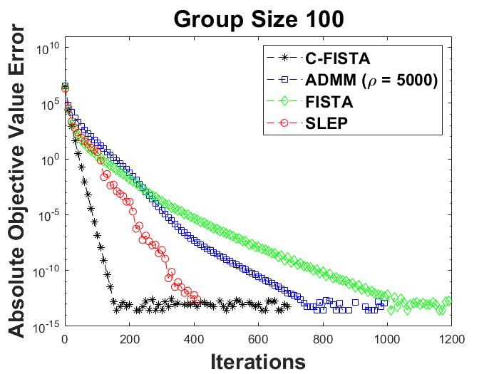
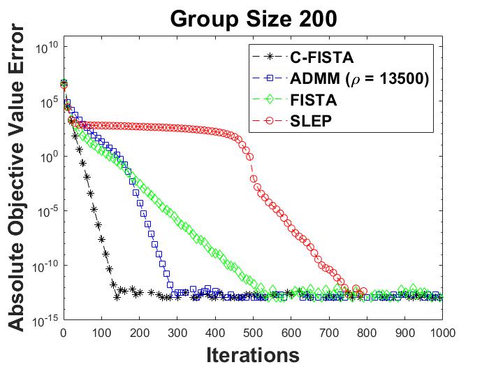
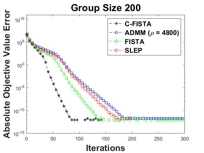
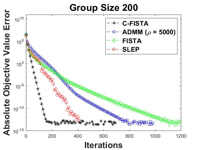
For comparing C-FISTA, SLEP, ADMM and FISTA (without backtracking) on the overdetermined Lasso models, we constructed synthetic data sets for testing in a manner similar to the process utilized in ZZST20 . For our tests of the group and sparse-group Lasso models, we randomly generated a data matrix from the standard normal distribution, and we formed three different subvector groups, and , where the subvectors in where of sizes and 200 respectively. Thus, in our experiments we let and had,
The response vectors for were formed as,
where each component of was drawn from the standard norm distribution, provided a scaling factor for the noise, and for with for the remaining subvector groups . We set the positive penalty parameters and to be equal and of a magnitude to ensure sparse but non-trivial solutions.
For the overlapping sparse-group Lasso model we constructed the data matrix in the same manner, and let the subvector groups be,
Thus, each of the adjacent subvectors in for overlapped with another subvector. The response vectors were constructed as done for the group and sparse-group Lasso models.
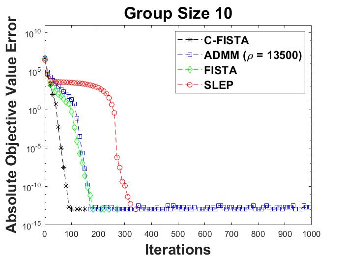
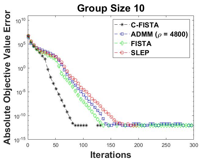
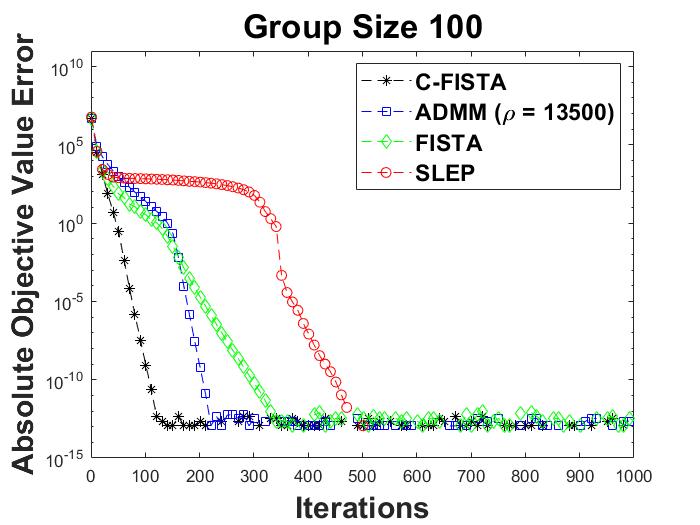
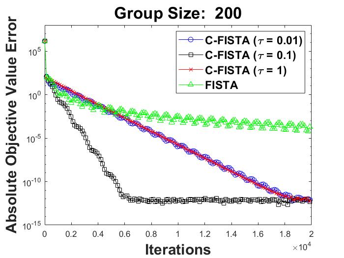
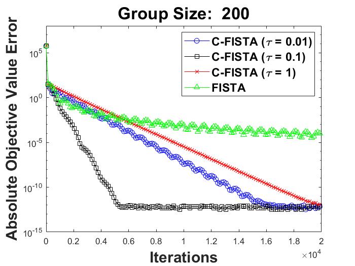
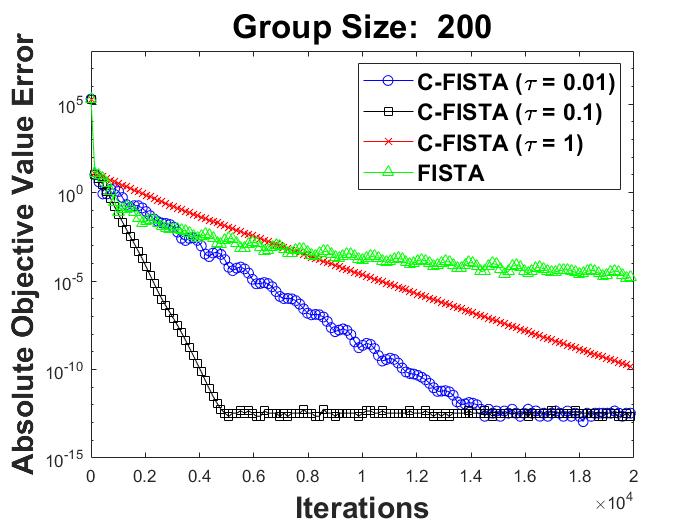
The overdetermined Lasso experiments were conducted in MATLAB R2021. Implementation of C-FISTA was as detailed in Sections 6.1.1, 6.1.2, and 6.1.3. From the SLEP software package SLEP we utilized: glLeastR.m, sgLeastR.m and overlapping_LeastR.m to solve the group, sparse-group and overlapping sparse-group Lasso models respectively. Sections 3, 7 and 9 of SLEP provide details for these first-order proximal gradient methods. FISTA, without backtracking, was applied as described in BT09 . All iterative sequences in the algorithms were initialized at zero. For comparison, all of the Lasso models were tested with the same data matrix and response vectors . Figure 1 displays the convergence results for C-FISTA, SLEP, ADMM and FISTA on the three Lasso models. In Figure 1, the y-axis measures the absolute difference from the optimal objective value at each iteration of the individual algorithms. We took the final value of the objective function of C-FISTA as the exact optimal solution which agreed, as can be seen in Figure 1, to within machine tolerance of the final iterates produced by each of the methods. Note, we fine-tuned the augmented Lagrangian parameter in the ADMM algorithm to achieve the optimal performance for the method.
The computational results displayed in Figure 1 clearly demonstrate the proven global linear convergence of C-FISTA. While ADMM, SLEP and FISTA all display linear convergence properties in some of the tests, C-FISTA significantly outperformed the other methods. Furthermore, C-FISTA maintained a robustness between the various Lasso models. While SLEP’s convergence rate suffered as the subvector group sizes increased in the group Lasso model, the convergence rate of C-FISTA did not suffer in the group or sparse-group Lasso models as the group sizes increased. Overall, the tests demonstrate C-FISTA’s effectiveness and robustness to varying subvector group sizes throughout the various Lasso formulations.
GL Tests
SGL Tests
OSGL Tests

6.2.2 Underdetermined Group Lasso Numerical Tests
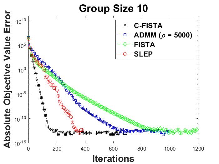
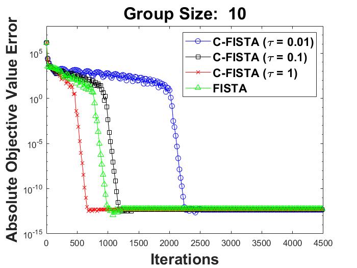
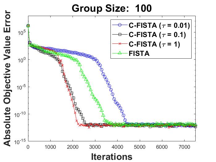
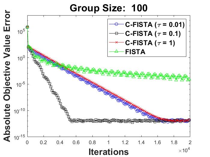
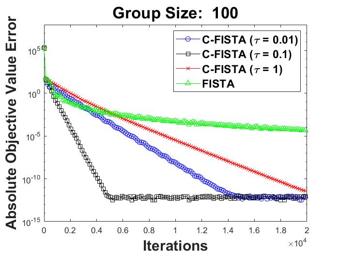
The second set of Lasso experiments focused on underdetermined data. In particular, the group Lasso model was studied with a rank deficient data matrix. With underdetermined data, the assumptions for Theorem 2.1 are not fully realized; however, as previously claimed and will be shown, in practice asymptotic linear convergence is still possible when the global assumptions (A2) and/or (A3) are not fully realized. To demonstrate this we conducted an extensive numerical experiment comparing FISTA, without backtracking, to C-FISTA on the group Lasso model with underdetermined data.
For the experiment, we let and . Therefore, the strong convexity and gradient Lipschitz constants for are , , and . The only remaining constant to compute is which by (A2) needs to satisfy,
for all . Since is not of full-column rank, this assumption cannot hold; however, choosing a small positive value for ensures the inequality will hold for a sufficient number of iterates generated by Algorithm 1. This enables C-FISTA to maintain its convergence though assumption (A2) is not formally satisfied.
In our underdetermined group Lasso experiments, we generated synthetic data matrices and response vectors as in Section 6.2.1. Randomly generated matrices with dimensions: and were constructed, and each of these group Lasso problem sizes were solved under the three subvector groupings from Section 6.2.1. We generated ten instances of these nine group Lasso settings and solved the models with FISTA and C-FISTA under three different parameter settings for . Table 1 displays the results for these ninety numerical experiments. Each entry in the table provides the average number of iterations for the respective algorithms to converge to within of the optimal objective value.
From Table 1 we observe C-FISTA is convergent for a range of values demonstrating a robustness to miss-specification. Of the different values for selected, only the selection of failed to converge after 20,000 iterations and this was only for the case and the group variable size was 200. Second, we note C-FISTA outperformed FISTA consistently with the best algorithm for each setting being C-FISTA with either or . A visual representation of the performance comparison is given in Figure 2. From the convergence plots we see C-FISTA would often display asymptotic linear convergence when the group sizes were 100 and 200 while FISTA would converge sub-linearly. When the group size was 10, irrespective of the dimension of the data matrix, C-FISTA and FISTA were comparable and demonstrated asymptotic linear convergence; however, with , C-FISTA converged between 300 and 500 iterations sooner on average then FISTA in this setting. These experiments demonstrate that C-FISTA maintains linear convergence properties even when some of the stated assumptions are not strictly met and showcases the robustness of the parameter to miss-specification.
| Data Dimension | |||||||||
| Method | 2500 x 5000 | 1200 x 5000 | 600 x 5000 | ||||||
| Group Size | Group Size | Group Size | |||||||
| C-FISTA | 10 | 100 | 200 | 10 | 100 | 200 | 10 | 100 | 200 |
| 2194 | 4069 | 15718 | 2170 | 13546 | 13288 | 2208 | 12014 | 11565 | |
| 1129 | 2202 | 5331 | 1202 | 4686 | 4436 | 1439 | 4088 | 4140 | |
| 624 | 2049 | 15517 | 833 | 14096 | 15473 | 1292 | 17327 | NaN | |
| FISTA | 945 | 3200 | NaN | 1284 | NaN | NaN | 1780 | NaN | NaN |
Dimension:
Dimension:
Dimension:


6.3 C-FISTA for Sparse-Group Logistic Regression
In this section we describe how to apply C-FISTA to solve the sparse-group logistic regression model,
As in the Lasso formulations, a decomposition must be chosen to tackle the regression model with C-FISTA. For continuity with the previous discussion, we will utilize the decomposition and Under these definitions for and , the sparse-group Lasso and sparse-group logistic regression models only differ with respect to their strongly convex term, so the procedure for solving the sparse-group logistic regression model with C-FISTA is very similar to Algorithm 3. Only two alterations to Algorithm 3 are required to solve the sparse-group logistic regression model. One, we must update in Algorithm 3 to be,
| (25) |
and second we require new estimates for the bounds of the Lipschitz and strong convexity constants and . Updating is straightforward, but obtaining tight upper and lower bounds on the Lipschitz and strong convexity constants can become a challenging task as mentioned previously. Algorithm 4 presents C-FISTA for solving the sparse-group logistic regression model. In our implementation of Algorithm 4, we fixed the Lipschitz and strong convexity parameters though backtracking procedures could be utilized.
Note, computing at each iteration is simple relative to because the subprobem (3) is decomposable into a minimization over and respectively. Since the minimization over contains no regularization terms, the first-order optimality conditions provide a simple update for .
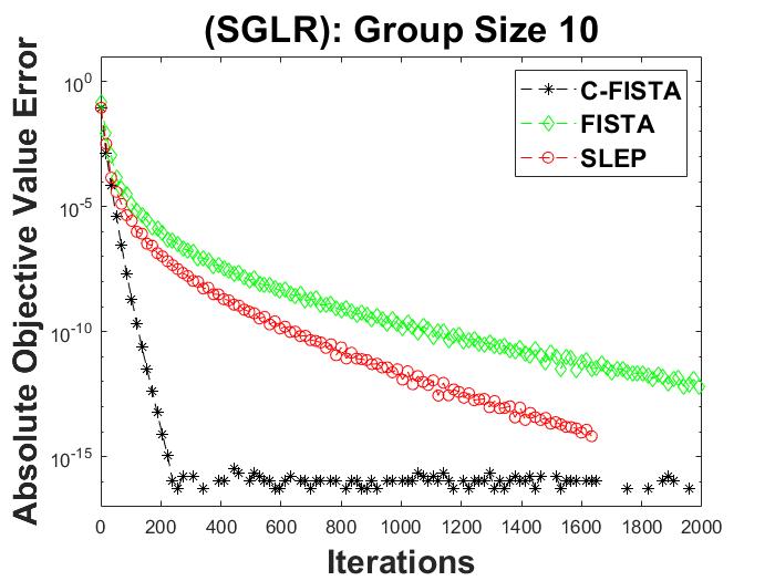
The astute observer will note is strictly instead of strongly convex making and leaving the necessary assumptions unsatisfied. Though this is technically true, C-FISTA is undeterred. As in the underdetermined group Lasso tests, this decomposition showcases the robustness of C-FISTA when the assumptions are not formally met. It is clear the sparse-group logistic regression model could be equivalently expressed as a constrained problem; therefore, by rewriting the model as an equivalent constrained problem, would become strongly convex on the problem domain; however, as is seen in Figure 3, C-FISTA outperforms both SLEP and FISTA without solving an equivalent model where the assumptions are formally satisfied.
6.4 Sparse-Group Logistic Regression Numerical Experiments
In this section, we describe the results of the numerical experiments on the sparse-group logistic regression model. The set-up for the numerical experiments on the sparse-group logistic regression model were similar to the set-up for the Lasso models in 6.2. We generated the data matrix from the standard normal distribution letting for be the rows of , and set where is the vector of all ones. We conducted three experiments from the generated data using the same subvector groups, , and , utilized in the group and sparse-group Lasso tests. We set in our tests to ensure a non-trivial solution with substantial sparsity.
In our experiments, we compared C-FISTA, SLEP and FISTA. With regards to SLEP, we utilized sgLogisticR.m, which is a first-order proximal gradient method, to solve the model. The computational results displayed in Figure 3 clearly demonstrate the proven global linear convergence of C-FISTA. In the logistic regression tests, C-FISTA was a vast improvement over both FISTA and SLEP converging well over a 1000 iterations sooner to within machine precision.
6.5 C-FISTA for Geometric Programming
In this section we discuss how to solve an instance of the geometric programming model described in Section 3. In particular, we focus on the group regularized geometric program,
| (26) |
where with and , , and for , and is a non-overlapping partition of the vector . Letting,
we can rewrite (26) in the format of our standard composite optimization model. From the characteristics of it follows is gradient Lipschitz on the problem domain. Additionally, will be strongly convex over the domain provided the vectors span . Note, this is a fairly weak condition if . Additionally, similar to our underdetermined group Lasso discussion, although constants and do not exist to satisfy the necessary constraints over the span of the constraint set, such constants exist which satisfy the necessary inequalities over the constraint set. By Taylor’s theorem and simple bounding we can see,
with and . Thus, with these values for and , along with appropriate estimates for the other parameters and , C-FISTA can be employed to solve instances of this subclass of geometric programs. The only difference in implementing C-FISTA for this problem class is a constrained optimization model of the form given in (23) must be solved to compute the proximal mapping. In our numerical experiments, we apply a simple projected gradient method to solve this subproblem to within a specified tolerance. We now present the numerical results from the geometric programming model.
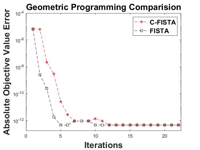
6.6 Geometric Programming Numerical Experiments
To test the performance of C-FISTA on (26), we generated random instances of the geometric programming model and compared Algorithm 1 to FISTA. For our randomly generated examples we let:
, , and . The values for the ’s and ’s were randomly computed using the randn command in MATLAB 2021b, and then they were transformed to ensure they held the proper sign. The ’s were additionally normalized so that the elements in each vector summed to negative one. This normalization was done to avoid extremely ill-conditioned problems.
Figure 4 displays an example result from our testing. For this problem, C-FISTA and FISTA would both converge exceptional fast often within 10-30 iterations. In general, FISTA would slightly outperform C-FISTA which might be a result of the parameter estimation. Nevertheless, C-FISTA demonstrated rapid convergence in a setting where the formal assumptions were not completely satisfied and a non-linear decomposition of the objective function was utilized.
7 Conclusions
In this paper we developed an accelerated composite version of FISTA, C-FISTA, which handles the composite optimization model (1) and is a generalization of GFISTA CC19 ; CP16 . We proved global linear convergence for C-FISTA without having a strongly convex objective function, and demonstrated through Fenchel duality the breadth of convex models which are solvable via C-FISTA in Section 4. In Section 6, we demonstrated through several numerical experiments C-FISTA was able to obtain linear convergence even in settings where the formal assumptions were not satisfied. Furthermore, C-FISTA outperformed ADMM, the software package SLEP and the seminal FISTA algorithm in both Lasso and logistic regression models.
The following lines of directions could be of interest as future research topics. First, the conditions underlying our global linear convergence results may be weakened. Second, one may further study possible adaptive schemes to implement C-FISTA without requiring the exact knowledge of the problem parameters. Finally, it is interesting to study how the new algorithm behaves beyond the scope of convex optimization.
8 Statements and Declarations
Funding. This material is based upon work supported by the National Science Foundation Graduate Research Fellowship Program under Grant No. 1839286. Any opinions, findings, and conclusions or recommendations expressed in this material are those of the author(s) and do not necessarily reflect the views of the National Science Foundation.
Competing Interests. The authors have no relevant financial or non-financial interests to disclose.
Data Availability. The datasets generated during and/or analysed during the current study are available from the corresponding author on reasonable request.
References
- (1) Auslender, A.: Asymptotic properties of the fenchel’s dual functional and their applications to decomposition problems. J. Optim. Theory Appl. 73, 427–449 (1992). DOI 10.1007/BF00940050
- (2) Beck, A., Shtern, S.: Linearly convergent away-step conditional gradient for non-strongly convex functions. Math. Program. 164, 1–27 (2017). DOI 10.1007/s10107-016-1069-4
- (3) Beck, A., Teboulle, M.: A fast iterative shrinkage-threshold algorithm linear inverse problems. SIAM J. Imaging Sci. 2, 183–202 (2009). DOI 10.1137/080716542
- (4) Boyd, S., Kim, S., Vandenberghe, L., Hassibi, A.: A tutorial on geometric programming. Optim. Eng. 8, 67–127 (2007). DOI 10.1007/s11081-007-9001-7
- (5) Burke, J.V., Ferris, M.C.: A gauss-newton method for convex composite optimization. Math. Program. 71, 179–194 (1995). DOI 10.1007/BF01585997
- (6) Calatroni, L., Chambolle, A.: Backtracking strategies for accelerated descent methods with smooth composite objectives. SIAM J. Optim. 29, 1772–1798 (2019). DOI 10.1137/17M1149390
- (7) Chambolle, A., Pock, T.: An introduction to continuous optimization for imaging. Acta Numer. 25, 161–319 (2016)
- (8) d’Aspremont, A., Scieur, D., Taylor, A.: Acceleration methods (2021). URL \urlhttps://arxiv.org/abs/2101.09545v1
- (9) Drusvyatskiy, D., Lewis, A.S.: Error bounds, quadratic growth, and linear convergence of proximal methods. Math. Oper. Res. 43, 919–948 (2018). DOI 10.1287/moor.2017.0889
- (10) Drusvyatskiy, D., Paquette, C.: Efficiency of minimizing compositions of convex functions and smooth maps. Math. Program. 178, 503–558 (2019). DOI 10.1007/s10107-018-1311-3
- (11) Florea, M.I., Vorobyov, S.A.: An accelerated composite gradient method for large-scale composite objective problems. IEEE Trans. Signal Process. 67, 444–459 (2019). DOI 10.1109/TSP.2018.2866409
- (12) Florea, M.I., Vorobyov, S.A.: A generalized accelerated composite gradient method: Uniting nesterov’s fast gradient method and fista. IEEE Trans. Signal Process. 68, 3033–3048 (2020). DOI 10.1109/TSP.2020.2988614
- (13) Fukushima, M., M, H., Nguyen, H.V., Strodiot, J.J., Sugimoto, T., Yamakawa, E.: A parallel descent algorithm for convex programming. Comput. Optim. Appl. 5, 5–37 (1996). DOI 10.1007/BF00429749
- (14) Gaffke, N., Mathar, R.: A cyclic projection algorithm via duality. Metrika 36, 29–54 (1989). DOI 10.1007/BF02614077
- (15) Han, S.P., Lou, G.: A parallel algorithm for a class of convex programs. SIAM J. Control Optim. 26, 345–355 (1988). DOI 10.1137/0326019
- (16) Hong, M., Luo, Z.Q.: On the linear convergence of the alternating direction method of multipliers. Math. Program. 162, 165–199 (2017). DOI 10.1007/s10107-016-1034-2
- (17) Jacob, L., Obozinski, G., Vert, J.P.: Group lasso with overlap and graph lasso. In: Proceedings of the 26th Annual International Conference on Machine Learning, ICML ’09, p. 433–440. Association for Computing Machinery, New York, NY, USA (2009). DOI 10.1145/1553374.1553431. URL \urlhttps://doi.org/10.1145/1553374.1553431
- (18) Liu, J., Ji, S., Ye, J.: SLEP: Sparse Learning with Efficient Projections. Arizona State University (2009). URL \urlhttp://yelabs.net/software/SLEP/
- (19) Meier, L., Geer, S., Buhlmann, P.: The group lasso for logistic regression. J. R. Stat. Soc. Ser. B. Stat. Methodol. 70, 53–71 (2008)
- (20) Necoara, I., Nesterov, Y., Glineur, F.: Linear convergence of first order methods for non-strongly convex optimization. Math. Program. 175, 69–107 (2019). DOI 10.1007/s10107-018-1232-1
- (21) Nesterov, Y.: A method for solving the convex programming problem with convergence rate . Proceedings of the USSR Academy of Sciences 269, 543–547 (1983)
- (22) Nesterov, Y.: Gradient methods for minimizing composite functions. Math. Program. 140, 125–161 (2013). DOI 10.1007/s10107-012-0629-5
- (23) Qin, Z., Scheinberg, K., Goldfarb, D.: Efficient block-coordinate descent algorithms for the group lasso. Math. Program. Comput. 5, 143–169 (2013). DOI 10.1007/s12532-013-0051-x
- (24) Rebegoldi, S., Calatroni, L.: Scaled, inexact and adaptive generalized fista for strongly convex optimization (2021). URL \urlhttps://arxiv.org/abs/2101.03915
- (25) Rockafellar, R.T.: Convex Analysis, 2nd edn. Princeton University Press, Princeton, New Jersey (1970)
- (26) Roos, K., Balvert, M., Gorissen, B.L., den Hertog, D.: A universal and structured way to derive dual optimization problem formulations. INFORMS J. Optim. 2, 229–255 (2020). DOI 10.1287/ijoo.2019.0034
- (27) Simon, N., Friedman, J., Hastie, T., Tibshirani, R.: A sparse-group lasso,. J. Comput. Graph. Statist. 22, 231–245 (2013). DOI 10.1080/10618600.2012.681250
- (28) Tibshirani, R.: Regression shrinkage and selection via the lasso. J. R. Stat. Soc. Ser. B. Stat. Methodol. 58, 267–288 (1996). DOI 10.1111/j.2517-6161.1996.tb02080.x
- (29) Wright, S.J.: Convergence of an inexact algorithm for composite nonsmooth optimization. IMA J. Numer. Anal. 10, 299–321 (1990). DOI 10.1093/imanum/10.3.299
- (30) Yuan, L., Liu, J., Ye, J.: Efficient methods for overlapping group lasso. IEEE Trans Pattern Anal Mach Intell. 35, 2104–2016 (2013). DOI 10.1109/TPAMI.2013.17
- (31) Yuan, M., Lin, Y.: Model selection and estimation in regression with grouped variables. J. R. Stat. Soc. Ser. B. Stat. Methodol. 68, 49–67 (2007). DOI 10.1111/j.1467-9868.2005.00532.x
- (32) Zhang, Y., Zhang, N., Sun, D., Toh, K.C.: An efficient hessian based algorithm for solving large-scale sparse group lasso problems. Math. Program. 179, 223–263 (2020). DOI 10.1007/s10107-018-1329-6
- (33) Zhou, X.: On the fenchel duality between strong convexity and lipschitz continuous gradient (2018). URL \urlhttps://arxiv.org/abs/1803.06573v1
- (34) Zhou, Z., So, A.M.C.: A unified approach to error bounds for structured convex optimization problems. Math. Program. 165, 689–728 (2017). DOI 10.1007/s10107-016-1100-9