Learning Augmented Online Facility Location

Abstract

Theorem 3.2 contains an error, which we are working to fix. For some alternative solutions developed in parallel to our work see [1, 2].

Following the research agenda initiated by Munoz & Vassilvitskii [3] and Lykouris & Vassilvitskii [4] on learning-augmented online algorithms for classical online optimization problems, in this work, we consider the Online Facility Location problem under this framework. In Online Facility Location (OFL), demands arrive one-by-one in a metric space and must be (irrevocably) assigned to an open facility upon arrival, without any knowledge about future demands.

We present an online algorithm for OFL that exploits potentially imperfect predictions on the locations of the optimal facilities. We prove that the competitive ratio decreases smoothly from sublogarithmic in the number of demands to constant, as the error, i.e., the total distance of the predicted locations to the optimal facility locations, decreases towards zero. We complement our analysis with a matching lower bound establishing that the dependence of the algorithm’s competitive ratio on the error is optimal, up to constant factors. Finally, we evaluate our algorithm on real world data and compare our learning augmented approach with the current best online algorithm for the problem.

1 Introduction

Online algorithms is a field that deals with algorithmic problems in which the input is not entirely known in advance, but rather arrives in a sequential way. The algorithm is required to make irrevocable decisions, only based on the input received at a given point, and to incur the corresponding irrevocable cost for each of them. Traditionally, in the analysis of online algorithms we assume, rather pessimistically, that an adversary always presents the algorithm with the worst case input. More precisely, the performance of online algorithms is evaluated by the competitive ratio [5], which is the worst-case ratio of total algorithm’s cost to the cost of a computationally unlimited optimal algorithm that is aware of the entire request sequence in advance.

On the other hand, one of the main goals in the field of machine learning is to predict the unknown based on data, and learn what the world looks like, rather than preparing for the worst that can happen. In an effort to exploit this, there has been a trend in recent years that tries to use machine learning predictions in order to deal with the inherent uncertainty in online algorithms, while still providing worst case performance guarantees. Specifically, one might think that directly using machine learning in online problems should enhance their performance, since by knowing, with some error, how the input looks like, we should be able to come up with almost optimal solutions/approximations. In reality, this turns out not to be true, since the error of the learner does not necessarily remain constant, and it could propagate during different phases of the algorithm and cause a much bigger error.

In a recent work, Lykouris and Vassilvitski [4] tried to formulate a framework to provide formal guarantees for these learning augmented online algorithms, in terms of consistency and robustness. Specifically, they require the algorithm to be near optimal, if the predictions are good enough (consistency), and for worse predictions, the competitive ratio should gracefully degrade to the worst case one (robustness). Generally, the idea of combining online algorithms with ML advice is that in the end, we are able to overcome the traditional worst-case analysis lower bounds, and we are guaranteed to get the best of both worlds. The ML-enhanced algorithm, given some predictions of total error $\eta$, is required to make choices online. In the end, following the ideas of [4] [6] [7], the guarantees are given as a function of $\eta$. Many online problems have already been studied under this framework, like ski rental, scheduling, the secretary problem, metrical task systems (MTS) and more, for which we have included a brief overview in the related work section. An important online problem not yet studied until now, is online facility location.

Online Facility Location.

In the online facility location problem, introduced by Meyerson [8], we are presented with a sequence of demands located in an underlying metric space. Each demand must be connected to an open facility upon arrival. Each facility has an opening cost, and cannot be closed once opened, and every demand pays its connection cost, which is the distance to the closest open facility. Our goal is to decide where to open the facilities and where to connect each arriving demand, while paying the minimum possible opening and connection cost. Meyerson presented a randomized algorithm that achieves a competitive ratio of $O(\log n/\log\log n)$, where $n$ is the number of demands. After Meyerson’s initial result, there has been continuing work on this problem, as well as many of its variants. We provide a brief list in the related work section.

1.1 Our Contribution

In this work, we study the online facility location problem in the framework of learning augmented online algorithms, following a similar approach to [6] in terms of evaluating the performance of our algorithms. We focus on the version with uniform facility costs, where the cost of opening a facility at any point of the underlying metric space is $f$. We present a simple randomized algorithm which for every demand, receives a prediction on the location of the optimal facility for this demand. The $\ell_{1}$ error $\eta_{1}$ is the sum, over all predictions, of their distance to the respective optimal facility, while we define the $\ell_{\infty}$ error ($\eta_{\infty}$) to be the maximum such distance. Our algorithm decides on whether to open a facility at the predicted location with probability proportional to the distance of the predicted location to the nearest open facility. This causes the algorithm to not undesirably open too many facilities in a certain area, since once a facility is opened, the probability of another one opening is decreased. In addition to proving the guarantee of our algorithm, we also show how to adapt the results of Antoniadis et al. [9] on MTS, in order to get the minimum competitive ratio of our proposed algorithm and the worst case Meyerson’s algorithm. Our main theorem is stated below.

Theorem (Main Theorem).

For $\eta_{1}=0$, there exists an algorithm that has competitive ratio $2$. For $\eta_{1}>0$, the competitive ratio is

$$O\left(\min\left(\frac{\log n}{\log\log n},\frac{\log\left(err_{\infty}\right)}{\log\left(err_{1}^{-1}\log\left(err_{\infty}\right)\right)}\right)\right)$$

where $n$ is the number of demand points, $err_{\infty}=\frac{n\eta_{\infty}}{f}$, $err_{1}=\frac{\eta_{1}}{f}$ and $f$ is the facility opening cost.

We note that in contrast to the initial work in this area, our algorithm does not require any hyper-parameter to be given to it up front. We also note that the dependence on $\eta_{\infty}$ implies that, even if the $\ell_{1}$ error is high, our algorithm can still be close to optimal, if the error is evenly distributed among the predictions, which also is the case in practical settings; our predictions will be a bit off, but no prediction will be off by a lot.

Our second result is a matching lower bound, on any randomized algorithm that uses these types of predictions. This implies that our proposed algorithm is optimal up to constants.

Theorem (Lower Bound).

No randomized algorithm can preform better than

$$\Omega\left(\frac{\log\left(err_{\infty}\right)}{\log\left(err_{1}^{-1}\log\left(err_{\infty}\right)\right)}\right)$$

where $n$ is the number of demand points, $err_{\infty}=\frac{n\eta_{\infty}}{f}$, $err_{1}=\frac{\eta_{1}}{f}$ and $f$ is the facility opening cost.

Finally, we experimentally evaluate our algorithms on both real-world and synthetic datasets for different types of predictions and errors.

1.2 Related work

Learning Augmented Algorithms.

This line of work was initiated by Munoz and Vassilvitski [3] and Lykouris and Vassilvitski [4], who formally introduced the notions of consistency and robustness. Purohit et al. [7] considered the ski rental problem and the non-clairvoyant scheduling problem, giving consistency and robustness guarantees that depend on a hyperparameter that has to be given to the algorithm in advance. Following this, Gollapudi and Panigrahi [10] also considered the ski rental problem in the setting of multiple predictors, while Wang et al. [11] considered the multi-shop ski-rental problem, a generalization of the classic ski rental problem. Lykouris and Vassilvitskii [4] studied the classical caching problem (also known in the literature as paging), and were able to adapt the classical Marker algorithm [12] to obtain a trade-off between robustness and consistency. Rohatgi [13] and Wei [14] subsequently presented simpler learning-augmented caching algorithms with improved dependence of their competitive ratios on the prediction errors.

Further results in online algorithms with machine learned advice include the work by Lattanzi et al. [15], who studied the restricted assignment scheduling problem, the work of Bamas et al. [16], who considered energy minimization problems, and the more general framework of online primal dual algorithms [17]. The work by Mitzenmacher [18] considered a slightly different scheduling/queuing problem, introducing also a different quality measure for evaluating algorithms, called “the price of misprediction”.

Adopting a slightly different model, Mahdian et al. [19] studied problems where it is assumed that there exists an optimistic algorithm (which could in some way be interpreted as a prediction), and designed a meta-algorithm that interpolates between a worst-case algorithm and the optimistic one. They considered several problems, including the allocation of online advertisement space, and for each gave an algorithm whose competitive ratio is also an interpolation between the competitive ratios of its corresponding optimistic and worst-case algorithms. However, the performance guarantee is not given as a function of the “prediction” error, but rather only as a function of the respective ratios and the interpolation parameter. In [6], the following online selection problems are studied: (i) the classical secretary problem, (ii) online bipartite matching with vertex arrivals and (iii) the graphic matroid secretary problem.

Online Facility Location.

The (metric uncapacitated) facility location is a classical optimization problem that has been widely studied in both the operations research and the computer science literature (see e.g., [20, 21], and more recently, in computer science, especially from the viewpoint of approximation algorithms, see e.g., [22]). Its online version has received significant attention since its introduction by Meyerson [8]. Meyerson initially presented a randomized algorithm and proved that its competitive ratio is $O(\log n)$. In subsequent work, Fotakis [23] gave a lower bound of $\Omega(\log n/\log\log n)$ and showed that Meyerson’s algorithm is asymptotically tight, matching the lower bound. Other algorithms were also given using different techniques; Fotakis [24] gave a deterministic primal-dual $O(\log n)$-competitive algorithm and Anagnostopoulos et al. [25] gave a deterministic $O(\log n)$-competitive algorithm using an idea for hierarchical partitioning of the metric space. For some follow up work on online facility location and its variants we refer the reader to the survey by Fotakis [26]. More recently, there has been continuing work on the dynamic variant of online facility location [27, 28, 29].

2 Preliminaries

In the following sections, we begin by introducing the online facility location problem, alongside some notation used in the rest of the technical sections. Then, we present a method, as a modification of Theorem 18 in [9], that allows to combine two (or more) online algorithms and get the best competitive ratio of them.

2.1 The Online Facility Location problem

In the online facility location problem (OFL), the input consists of a sequence of demands $\mathcal{D}$ in a metric space $(\mathcal{M},d)$. The demands arrive one at a time and must be assigned irrevocably to an open facility upon arrival. In response to the demands sequence $v_{1},v_{2},\cdots,v_{i}$, the online algorithm maintains a facility configuration denoted by $\mathcal{F}_{i}$.

When a new demand $v_{i}$ arrives, the algorithm decides whether to assigned it to an existing facility or a new one, $c_{new}$. If the algorithm opens a new facility, the facility cost increases by $f$, and $\mathcal{F}_{i}=\mathcal{F}_{i-1}\cup\{c_{new}\}$. Finally, the demand $v_{i}$ is assigned to nearest facility in $\mathcal{F}$, and the assignment cost increases by $d(v_{i},\mathcal{F}_{i})$. The goal is to minimize the overall assignment and facility opening cost

$$f\cdot|\mathcal{F}_{n}|+\sum_{v_{i}\in\mathcal{D}}d(v_{i},\mathcal{F}_{i})$$

The cost incurred by the optimal solution is denoted by OPT, while $Asg^{*}$ is the respective assignment cost. In addition, OFL and PredFL denote the Meyerson’s algorithm and the presented algorithm respectively.

2.2 Predictions

Upon the arrival of a demand $v$, the algorithm receives a prediction $\hat{c}_{v}$ concerning the optimal facility $c^{*}_{v}$ at which $v$ is assigned in the optimal solution. The overall error of the predictions sequence is defined as the $\ell_{1}$ norm of the distances $d(\hat{c}_{v},c^{*}_{v})$. Thus, $\eta_{1}=||\eta||_{1}=\sum_{v}\eta_{v}$ denotes the overall $\ell_{1}$-error, and $\eta_{\infty}=||\eta||_{\infty}=\max\limits_{v}\eta_{v}$ denotes the $\ell_{\infty}$-error.

2.3 Combining two online algorithms for OFL

Inspired by a method for combining online algorithms for metrical task systems that appeared in [9], we provide here an adaptation of that method that makes it applicable to our setting. Suppose that we have $2$ algorithms $A_{0}$ and $A_{1}$ for the OFL problem. Our goal is to construct a new online algorithm $A$, that has cost $O(\min\{cost(A_{0}),cost(A_{1})\})$. We will reduce this setting to the well known cow path problem, and prove a more specific bound of $13\cdot\min\{cost(A_{0}),cost(A_{1})\}$ for the cost of our algorithm.

Input: MIN ($A_{0},A_{1}$)

1 $prev\_fcost=[0\;\;0]$

2 $prev\_cost=[0\;\;0]$

3 $i=0$

4 $\ell=0$

5 repeat

6      

7      while $cost(A_{i})\leq 2^{\ell}$  do

8             Follow $A_{i}\quad$ # $cost(A_{i})$ denotes the cost that $A_{i}$ has incurred so far

9       end while

10      

11      if $fcost(A_{1-i})-prev\_fcost[1-i]>cost(A_{i})+prev\_cost[1-i]$ then

12             $\ell=\ell+1\quad$ # $fcost(A_{i})$ denotes the facility cost that $A_{i}$ has incurred so far

13            

14       else

15             $prev\_fcost=[fcost(A_{0})\;\;fcost(A_{1})]$

16             $prev\_cost=[cost(A_{0})\;\;cost(A_{1})]$

17             $\ell=\ell+1$

18             $i=i+1\mod 2$

19            

20       end if

21      

22until the end of the input;

Algorithm 1 MIN: Combine two OFL algorithms

Theorem 2.1.

Given $2$ online algorithms $A_{0},A_{1}$ for the OFL problem, the algorithm $\textsc{MIN}(A_{0},A_{1})$ has cost at most $13\cdot\min\{cost_{A_{0}}(I),cost_{A_{1}}(I)\}$ for any input sequence $I$.

Proof Sketch.

The idea behind the proof is inspired by the classical online algorithm for the cow path problem. In line $7$ of Algorithm 1, we copy exactly the decisions of one of the two algorithms available. However, when we switch from one of the algorithms to the other one, we need to incur a certain cost in order to reach the state (i.e., the set of open facilities) the new algorithm would be in. In our case, this is the cost of the facilities that the new algorithm would have opened since the last time our combined algorithm was following it. The idea is that we only follow the decisions of some algorithm, while it has not paid cost more than a constant factor larger than the alternative one. In this way, we can guarantee that at any point in the demand sequence, our combined algorithm incurs a cost which is within a constant factor of the minimum cost of the two algorithms. The main technical part of the proof is to show that the switching costs are not significant (i.e they are also within a constant factor from the minimum cost). This is shown by bounding from above the total cost of the combined algorithm by a geometric sum.

The full proof of the theorem is deferred to the appendix. ∎

3 PredFL: Learning Augmented Facility Location

In this section we describe the algorithm that uses predictions to solve an online facility location problem, and show the guarantees this algorithm achieves. Intuitively, the algorithm works in a similar way to Meyerson’s OFL [8]; every time a demand-prediction pair arrives, we open a facility at the prediction with probability proportional to the distance of the prediction from the already open facility. This is formally described in Algorithm 2. Initially we show that when the error is $0$, we get a solution constant away from the optimal. Then we proceed to show our main theorem (Theorem 3.2).

Input: New demand $v_{i}$ arrived at time $i$

1 $\mathcal{F}=\emptyset$ (Set of open facilities)

2 foreach New demand $v$ and prediction $\hat{c}_{v}$ do

3       $c_{open}=\operatorname*{arg\,min}\limits_{c\in\mathcal{F}}d(v,c)$

4       if $d(v,\hat{c}_{v})>f$ then

5             Open facility at $v$

6             $\mathcal{F}=\mathcal{F}\cup\{v\}$

7       else

8             $r_{v}=d(c_{open},\hat{c}_{v})$

9             Open facility at $\hat{c}_{v}$ w.p. $\min\{1,\frac{r_{v}}{f}\}$

10             If the last step was successful, $\mathcal{F}=\mathcal{F}\cup\{\hat{c}_{v}\}$

11       end if

12      

13 end foreach

Algorithm 2 PredFL: Facility Location with Predictions

Theorem 3.1 (Consistency).

When $\eta_{1}=0$, algorithm 2 has competitive ratio $2$.

It is clear that for one optimal cluster the algorithm achieves the exact optimal. The factor $2$ comes from the case of multiple optimal clusters; when a facility has already opened on an optimal center, each one of the next optimal centers needs to “accumulate potential” $f$ before opening, and then opens. We defer the proof of this theorem to subsection A.2 of the Appendix.

In the general case, where the error is positive, we show the following general result.

Theorem 3.2.

Algorithm 2, when $\eta_{1}>0$ has competitive ratio

$$O\left(\min\left(\frac{\log n}{\log\log n},\frac{\log\left(err_{\infty}\right)}{\log\left(err_{1}^{-1}\log\left(err_{\infty}\right)\right)}\right)\right)$$

where $n$ is the total number of demands, $err_{\infty}=\frac{n\eta_{\infty}}{f}$ and $err_{1}=\frac{\eta_{1}}{f}$.

For the analysis of this theorem, on a high level, we divide the space around each optimal center in concentric rings, each corresponding to one phase of the algorithm. In each ring there are the close demands, that contribute to the assignment cost, and the far ones, that have higher probability towards opening a facility. The analysis works by charging the close ones towards the $\ell_{1}$-error, and the far ones towards the opening of a facility closer to the optimal center. The structure is depicted in Figure 1. In order to show the main theorem, we need the following two lemmas, bounding the cost of close and far demands.

Lemma 3.3 (Far demands).

In the construction of Theorem 3.2, denote by $C_{far}$ the total cost incurred by far demands and $\ell$ the total number of phases, then $\mathbb{E}\left[C_{far}\right]\leq Asg^{*}_{far}+\ell\frac{3\lambda}{(\lambda-1)}f$

Lemma 3.4 (Close demands).

In the construction of Theorem 3.2, denote by $C_{close}$ the total cost incurred by close demands, then $\mathbb{E}\left[C_{close}\right]\leq Asg^{*}_{close}+(2m\lambda+1)\eta_{1}$

The proofs of both lemmas are defered to section A.2 of the Appendix. We now formally prove the main theorem.

Proof of Theorem 3.2.

We focus the analysis on single optimal center $c^{*}$, in Lemma A.2 in the Appendix we show why this assumption is without loss of generality. The area surrounding the optimal center $c^{*}$ is divided into concentric rings (with geometrically increasing radii) centered at $c^{*}$ called zones (see also Figure 1), where each zone $i$ contains all the demands $v$ whose prediction $\hat{c}_{v}$ is at distance $\frac{\eta_{op}}{m^{i+1}}\leq d(\hat{c}_{v},c^{*})\leq\frac{\eta_{op}}{m^{i}}$. Each of the zones corresponds in one Phase of the algorithm; Phase $i$ ends, when a facility is opened in zone $i$.

Denote by $\ell$ the total number of zones and observe that for the demands with predictions at distance $d(c^{*},\hat{c}_{v})\leq f/n$, even if we charge them all with error $f/n$, we at most double the final cost. Therefore we want the innermost zone to be

$$\frac{{\eta_{op}}}{m^{\ell}}\approx\frac{f}{n}.$$ (1)

Consider at some phase of the algorithm that the closest (to the center) open facility is at zone $i-1$. In each phase we split the demands that arrive in two types; the close ones whose prediction is within $\lambda$ of Zone $i-1$ and the far ones whose prediction is at least $\lambda$ far from Zone $i-1$, and therefore from the currently open facility. The parameters $m$ and $\lambda$ will be chosen at the end of the analysis. The structure is depicted on figure 1.

Observe that when a facility is opened at zone $i$, all demands $x$ that have their prediction on the outside of this zone, cannot incur cost more than $\mathbb{E}\left[cost_{x}\right]\leq d^{*}(x)+3\eta_{x}$, which comes from Lemma A.1 and the fact that $r_{x}\leq\eta_{x}+\eta_{op}^{(i)}\leq 2\eta_{x}$.

Figure 1: Concentric zones around the optimal center

Formally, we bound the cost of each of the two types of demands that arrive. Assume that the algorithm is at Phase $i$. Denote by $f_{op}^{i}$ and $\eta_{op}^{(i)}$ the current open facility closest to $c^{*}$ and its error respectively. From the definition of a Phase, we know that

$$\frac{\eta_{op}}{m^{i}}\leq\eta_{op}^{(i)}\leq\frac{\eta_{op}}{m^{i-1}}$$ (2)

Denote by $C_{far}$ and $C_{close}$ the cost incurred by the demands that are far and close respectively and by $\ell$ the total number of phases. Using Lemmas 3.3, 3.4 to bound the expected cost of the far and close demands we get:

$$\mathbb{E}\left[ALG\right]=\mathbb{E}\left[C_{close}\right]+\mathbb{E}\left[C_{far}\right]\leq Asg^{*}+(2m\lambda+1)\eta_{1}+\ell\frac{3\lambda}{(\lambda-1)}f$$

Setting $\lambda$ to be any constant $\lambda>1$ we get that the cost of the algorithm is $O(m\eta_{1}+\ell f)$. We want to set $m$ such that $m\eta_{1}=\ell f$. Substituting $\ell$ in equation 1, rearranging and observing that in the worst case $\eta_{op}=\eta_{\infty}$ we get

$$m\log m=\frac{f}{\eta_{1}}\log\left(\frac{\eta_{\infty}n}{f}\right).$$

This gives $m=\exp(W_{0}(B))$ where $B=\frac{f}{\eta_{1}}\log\left(\frac{\eta_{\infty}n}{f}\right)$, and $W_{0}(x)$ is the Lambert $W$ function. Using the bound on $W_{0}(x)$ for $x>e$, given in [30], we get that $m=\Theta\left(\frac{B}{\log B}\right)$, which gives the second part of the competitive ratio in the theorem statement. Combining this with Theorem 2.1, and running Meyerson’s algorithm in parallel, we get the theorem statement. ∎

4 Lower Bound

After presenting a learning augmented algorithm, one might reasonably wonder whether it achieves the optimal competitive ratio. That is, if there is an alternative algorithm that achieves even lower competitive ratio. Fortunately, we prove that it is not possible up to constants, by providing a lower bound on any randomized algorithm that uses similar predictions.

Specifically, we prove that given a total error $\eta_{1}$, it is possible to construct a distribution of inputs and predictions, so that the cost any deterministic algorithm incurs, is at least that of the algorithm’s guarantee presented in Theorem 3.2. The result follows from the Yao’s principle which extends the lower bound to any randomized algorithm (Chapter 8.4 of [5] and [31]). We emphasize that due to its construction, this lower bound is independent of any algorithm.

Theorem 4.1.

For any error value $\eta_{1}>0$, there exists an instance of demands and predictions, with total $\ell_{1}$ error equal to $\eta_{1}$, such that no algorithm can achieve a competitive ratio better than

$$\Omega\left(\frac{\log\left(err_{\infty}\right)}{\log\left(err_{1}^{-1}\log\left(err_{\infty}\right)\right)}\right)$$

where $err_{\infty}=\frac{n\eta_{\infty}}{f}$ and $err_{1}=\frac{\eta_{1}}{f}$.

Proof.

The construction of the lower bound is similar to the online facility location lower bound described in [23]. Specifically, the metric space is a binary Hierarchical Well-Separated Tree $T$ of height $\lambda=m\,\alpha$, where $\alpha=\eta_{1}/f$. The distance of the root to its children is $\frac{m^{\lambda-1}}{\alpha}$, and the edge lengths along a path from the root to a leaf decrease by a factor of $m$ at every level. The distance of any vertex at level $i$ to its children is $m^{(\lambda-1)-i}/\alpha$. The construction is shown in Figure 5 of the appendix. We denote by $T_{v}$ the subtree of $T$ rooted at a vertex $v$. Observe that the following two properties hold

1. The distance of a level-$i$ vertex $v_{i}$ to any vertex in $T_{v_{i}}$ is at most $\frac{m^{\lambda-i-1}}{\alpha}\frac{m}{m-1}$

2. The distance to any vertex not in $T_{v_{i}}$ is a least $m^{\lambda-i}/\alpha$

Constructing the demand sequence:

The demand sequence is divided into $\lambda+1$ phases. Phase $0$ consists of $1/\alpha$ demands at the root $v_{0}$ of $T$. After the end of phase $i-1,\ 0\leq i-1\leq\lambda$, if $v_{i-1}$ is not a leaf, the adversary selects $v_{i}$ uniformly at random from the two children of $v_{i-1}$. In the next phase, $i$, $\frac{m^{i}}{\alpha}$ demands arrive at the vertex $v_{i}$. Since $n$ is the total number of demands, we require that

$$n=\sum_{i=0}^{\lambda}\frac{m^{i}}{a}=\frac{1}{\alpha}\frac{m^{\lambda+1}-1}{m-1}\approx m^{\lambda}/\alpha$$ (3)

Constructing the predictions sequence:

Similarly, the predictions sequence is divided into $\lambda+1$ phases. For each demand of phase $i$, we get prediction $\hat{c}_{v_{i}}$ at distance $\alpha\,d^{*}_{v_{i}}$ from the optimal center. Observe that since the length of the edges increases proportionally to $1/\alpha$, each prediction $\hat{c}_{v_{i}}$ is located along the edge connecting the vertices $v_{i}$ and $v_{i+1}$, as shown in Figure 5.

Cost of the optimal:

The optimal solution opens a single facility at $u_{h}$. From Property $1$ observe that in each phase $i$ the optimal incurs assignment cost at most $\frac{m^{i}}{\alpha}\,\frac{m^{(\lambda-1)-i}}{\alpha}\frac{m}{m-1}=\frac{m^{\lambda-1}}{\alpha^{2}}\frac{m}{m-1}$, since $u_{h}\in T_{v_{i}}\ \forall\ 0\leq\ i<h$. Therefore, the overall optimal cost is at most $f+\lambda\frac{m^{\lambda-1}}{\alpha^{2}}\frac{m}{m-1}=f+\frac{m^{\lambda}}{\alpha}\frac{m}{m-1}$, using that $\lambda=m\alpha$. Setting $f=\frac{m^{\lambda}}{\alpha}$ we get

$$\textsc{OPT}\leq 2f\frac{m}{m-1}.$$ (4)

Cost of any algorithm:

Denote by ALG any deterministic algorithm. We abuse notation and use ALG to also denote the algorithm’s cost. At the end of any phase $i$, ALG knows that there exists a facility in $T_{v_{i}}$, but it cannot tell in which of $T_{v_{i}}$’s subtrees the facility should be. We fix the adversary’s choices up to the end of the phase $i$ and consider the assignment cost incurred by ALG for demands and facilities not in $T_{v_{i+2}}$, i.e. $\mathbb{E}\left[T_{v_{i}}\setminus T_{v_{i+2}}|\,v_{0},v_{1},\cdots,v_{i}\right]$, and distinguish the following cases

• ALG has no facilities in $T_{v_{i}}$ at the moment the first demand at $v_{i+2}$ arrives:
  The assignment cost for the demands at $v_{i},v_{i+1}\in T_{v_{i}}\setminus T_{v_{i+2}}$ is at least $\frac{m^{i}}{\alpha}\frac{m^{\lambda-i}}{\alpha}+\frac{m^{i+1}}{\alpha}\frac{m^{\lambda-(i+1)}}{\alpha}=2\,\frac{m^{\lambda}}{\alpha^{2}}$.

• ALG has at least one facility in $T_{v_{i}}\setminus T_{v_{i+2}}$:
  ALG opens a single facility at $v_{i+1}$, as the prediction $\hat{c}_{v_{i}}$ reveals the true subtree $T_{v_{i+1}}$ where the optimal center is located in and incurs an assignment cost only for the demands at $v_{i}$.

However, with $1/2$ probability the adversary selects $v_{i+2}$ so that at least one of ALG’s facilities is not included in $T_{v_{i+2}}$, therefore the algorithm’s cost is at least $f/2$ for every two phases. Taking into account only the first $\lambda$ phases, we get $\textsc{ALG}\geq\frac{\lambda}{4}f$. Combining this with equation (4) we get a competitive ratio of $\Omega(\lambda)=\Omega(m\,\frac{\eta_{1}}{f})$. In this construction we have that $\eta_{1}/\eta_{\infty}=m$, and using that in equation (3), given also the definition of $\alpha$ and that $\lambda=\alpha m$, and taking the $\log$ we get

$$m\log m-\frac{\eta_{1}}{f}\log m=\frac{f}{\eta_{1}}\log\left(\frac{\alpha n\eta_{\infty}}{f}\right)$$ (5)

Observing that $\eta_{1}=Asg^{*}\approx f$ in our construction, the first term is within constant of $m\log m$, and using a similar argument to the upper bound (Theorem 3.2), we get the theorem. ∎

5 Experiments

In this section we describe the setup for our experiments, the datasets we used and the way we created the predictions.

Datasets

We use the following datasets, also used in [28]. All datasets are equipped with the Euclidean metric, and for the [32, 33] datasets we restricted our experiments to the first 20K points.

• The CoverType data set [32], from the UCI repository with 58K instances of 54 dimensions.

• The US Census data set [33], from the UCI repository with 2.5 million instances of 68 dimensions.

• A synthetic dataset, created by sampling 2K points uniformly at random on the grid $[10^{6},10^{6}]$.

Our code is written in Python and the experiments were executed on a Debian virtual machine on Google Cloud with 16vCPUs and $30GB$ of memory. The code is included in the supplementary material.

Predictions

To generate the predictions, we first calculate the optimal offline solution given the demands on the metric space. In order to calculate the optimal solution, we solved the LP- relaxation of facility location, using Gurobi version $9$, and using deterministic rounding we obtained a $6$-approximate integer solution. Specifically for the CoverType and US Census datasets, we split them into batches of size $1K$ and for each batch we solved the offline optimal. We used the following three methods to generate the predictions of each demand.

1. alpha_predictor: the prediction is the point which is located on the line connecting the demand $x$ and the corresponding optimal center $c^{*}$ at distance $\alpha\cdot d(x,c^{*})$ from $x$.

2. alpha_gaussian_predictor: operates in a similar way. The prediction is at distance $g_{\alpha}\cdot d(x,c^{*})$, where $g_{\alpha}\sim\mathcal{N}(\alpha,std)$ and $\alpha,std$ are given as parameters.

3. perturb_gaussian_predictor: uses the same parameters as the second method, but the prediction is generated by $\vec{p}=\vec{c}+g_{\alpha}\cdot(\vec{d}-\vec{c})$, where $\vec{c},\vec{d},\vec{p}$ are the vectors of the optimal center, the demand and the prediction respectively.

Graphs

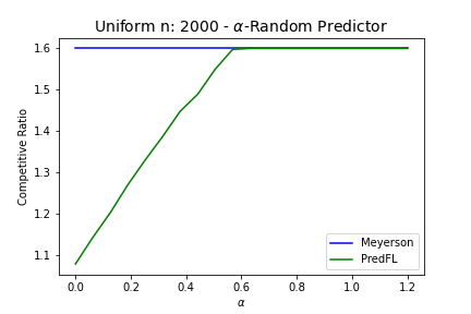
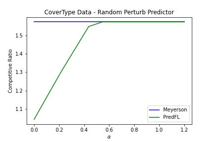
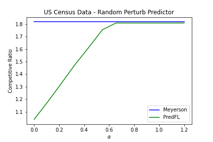
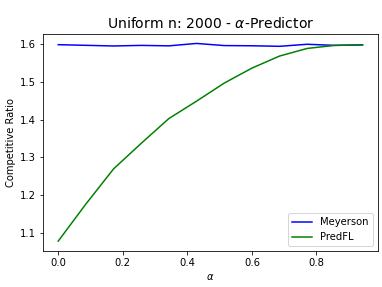
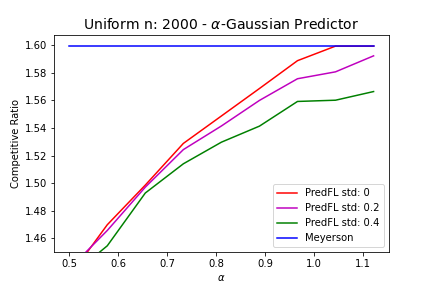
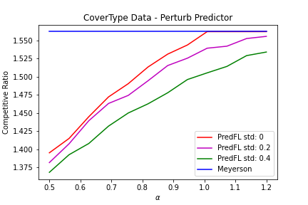
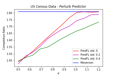
In the following graphs we compare the competitive ratio of Meyerson’s online facility location algorithm (Meyerson) and our proposed algorithm with predictions (PredFL). The costs of each algorithm have been calculated using the worst case scenario. In all three figures we observed the same behavior in terms of the competitive ratio. Our algorithm’s competitive ratio converges smoothly to the Meyerson’s as the parameter $\alpha$ increases from $0$ to $1$.

An interesting finding of our experiments (the corresponding plots are deferred to the appendix) is that in alpha_gaussian_predictor, the total cost of the online algorithm is slightly decreasing with the standard deviation. On the one hand, increasing the standard deviation might cause $\eta_{\infty}$ to increase. On the other hand, some of the subsequent far predictions are bound to be closer to the optimal center, and due to our facility opening rule these predictions are more likely to turn into new facilities, due to their increased distance to the nearest open facility. Interestingly, the latter effect dominates, which results in a slightly decreased competitive ratio, as the standard deviation increases. This is in accordance with our lower bound construction, where $d(x,f_{open})/d(\hat{f}_{x},f_{open})=\alpha$, for all demands $x$.

Figure 2: A comparison of PredFL’s and Meyerson’s competitive ratio for different predictors and errors.

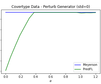
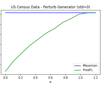
6 Conclusions

In this work, we are the first to study the online facility location problem under the framework of learning-augmented algorithms. Adapting Meyerson’s algorithm, we present a simple randomized algorithm that incorporates predictions on the position of the optimal facility and achieves a sublogarithmic, in the prediction error, competitive ratio. We also showed that the competitive ratio of our algorithm is optimal, up to constant factors, by proving a matching lower bound on all randomized algorithms. We also experimentally evaluated our results on both synthetic and real life datasets, and confirmed the theoretical results.

We showed that existing online algorithms techniques can be adapted to work in the learning augmented framework, and can overcome the worst-case lower bounds, while providing a smooth way to transition from near optimal competitive ratio (when predictions are good enough) to the worst case (when predictions are bad). This line of work can be extended to other online network design problems, such as the online Steiner tree problem.

Appendix A Appendix

A.1 Proofs of Section 2

proof of Theorem 2.1.

For any fixed value of $\ell$ (suppose wlog that we are following algorithm $A_{0}$ for that value of $\ell$), we distinguish $2$ cases :

• Case $1$: The cost of the new facilities that the algorithm $A_{1}$ would have opened between the $(\ell-1)$-th and $\ell$-th iteration is smaller than the total cost that the algorithm $A_{0}$ has incurred after the completion of the $\ell$-th iteration plus the cost the algorithm $A_{1}$ has incurred after the completion of the $(\ell-1)$-th iteration (i.e the condition of the IF statement on line $9$ is not satisfied). In this case, our argument and algorithm becomes quite similar to the one in Section 2.1 of [9] expressing the cost as a geometric sum.

• Case $2$: The condition of the IF statement on line $9$ is satisfied and therefore the algorithm that is being followed does not change. In this case, we distinguish the following two subcases:

  • a. The total cost of algorithm $A_{1}$ is at most $2^{\ell+1}\leq 4\cdot cost(A_{1})$, where $cost(A_{1})$ denotes the current cost. In this case, the switch would have been beneficial to the algorithm. However, it is now guaranteed to happen at $\ell+1$ and the extra cost incurred is not more that $2^{\ell+1}\leq 4\cdot cost(A_{1})\leq 4\cdot\min\{cost_{A_{0}}(I),cost_{A_{1}}(I)\}$. We get the desired result by adding the bound of the traditional cow path problem, which is $9\cdot\min\{cost_{A_{0}}(I),cost_{A_{1}}(I)\}$.

  • b. The total cost of algorithm $A_{1}$ is more than $4\cdot cost(A_{1})$. In this case, not switching is beneficial to the algorithm and therefore, we can still upper bound the cost by the geometric sum in case $1$.

To finish the proof, we distinguish the following cases:

1. For every value of $\ell$, we are in case $1$. In this case, the “else” part of the IF statement in line $9$ is always followed, and the total cost of the combined algorithm $MIN$ will be:

   $$2\cdot\sum_{i=0}^{\ell_{max}}2^{i}+OPT$$

   where $OPT=\min\{cost_{A_{0}}(I),cost_{A_{1}}(I)\}$ and $\ell_{max}=\lfloor\log(OPT)\rfloor+1$ Thus, we get that the cost will be at most $9\cdot OPT$.

2. For some values of $\ell$, we are in case $2b$. In this case, if the “else” part of the IF statement in line $9$ had been followed, the algorithm would incur an extra cost of $3\cdot 2^{\ell}$, which does not have to “pay” now. Therefore, if only either case $1$ or case $2b$ are ever encountered, the cost in still bounded by $9\cdot OPT$.

3. For some value of $\ell$, we are in case $2a$. Note this can only happen once as the algorithm terminates shortly after. In this case, as discussed above, an extra cost of at most $4\cdot OPT$ can be incurred.

Combining the above, we deduce that the total cost of algorithm $MIN(A_{0},A_{1})$ is at most $13\cdot\min\{cost_{A_{0}}(I),$ $cost_{A_{1}}(I)\}$ ∎

A.2 Proofs of Section 3

Proof of Theorem 3.1.

If $\eta_{1}=0$ this implies that $\eta_{x}=0$ for all points $x$ that arrive, therefore every prediction corresponds to an optimal cluster. Facilities that will open are on some optimal cluster since line $4$ of the algorithm is never true, and facilities only open at predictions.

One optimal cluster:

Initially observe that if there is only one optimal center, or if for any two optimal centers $i,j$ holds that $d(c^{*}_{i},c^{*}_{j})>2f$, then Algorithm 2 gives exactly the optimal. This happens since the predictions are on the optimal center, and are independent (since the distance from already open optimal center is more than $f$).

Many Optimal Clusters:

In this case, the opening probability may change depending on the position of the closest already open facility to the demand that arrived. We included a small example with 3 optimal centers in figure 3.

Figure 3: Example for $3$ optimal centers and $\eta_{1}=0$.

Denote by $X_{t}^{i}=\mathbbm{1}\{$Center $i$ is open at time $t\}$, and let $c_{i}^{*}$ be an arbitrary optimal cluster. We bound the cost of the cluster until the optimal center opens. Every new demand belonging to $c^{*}_{i}$ that arrives at time $t$, opens the optimal cluster with probability $r_{c(t)}/f$ where $r_{c(t)}=d(c^{*}_{i},c^{*}_{t})$. Observe that every time the demand fails to open a facility at $c^{*}_{i}$, by triangle inequality the extra cost incurred is $r_{c(t)}$. Let $T$ be the time that a facility opens at $c^{*}_{i}$ , then the cost incurred until $T$ is

$$\sum_{t=1}^{\infty}X_{t}^{i}r_{c(t)}=\sum_{t=1}^{T}r_{c(t)}\\$$ (6)

Observe that $\sum_{t=1}^{T}X_{t}^{i}=1$ by the definition of $T$ and the random variables $X_{t}^{i}$, therefore $\mathbb{E}_{T,X_{t}^{i}}\left[\sum_{t=1}^{T}X_{i}\right]=1$, but

$$\mathbb{E}_{T,X_{t}^{i}}\left[\sum_{t=1}^{T}X_{i}\right]=\mathbb{E}_{T}\left[\sum_{t=1}^{T}\mathbb{E}_{X_{t}^{i}}\left[X_{t}^{i}\right]\right]=\mathbb{E}_{T}\left[\sum_{t=1}^{T}\frac{r_{c(t)}}{f}\right].$$

This implies that $\mathbb{E}_{T}\left[\sum_{t=1}^{T}r_{c(t)}\right]=f$, and using equation (6) we get that the extra cost paid is $f$. Observing that the optimal solution also has cost at least $f$ we get the theorem. ∎

Proof of Lemma 3.4, Close demands.

Recall that for phase $i$ from the definition of Phase we have that

$$\frac{\eta_{op}}{\lambda m^{i}}\leq\eta_{x}\leq\frac{\eta_{op}}{m^{i}}.$$ (7)

Using Lemma A.1 we have that for any close demand $x$ arriving in Phase $i$ the cost is

$$\mathbb{E}\left[\text{cost }x\right] \leq d^{*}(x)+r_{x}+\frac{r_{x}}{f}\eta_{x}+\left(1-\frac{r_{x}}{f}\right)\eta_{op}^{(i)}$$

$$\leq d^{*}(x)+(m\lambda+1)\eta_{x}+\frac{r_{x}}{f}\eta_{x}+\left(1-\frac{r_{x}}{f}\right)\eta_{op}^{(i)} \text{Since }r_{x}\leq\eta_{op}^{(i)}+\eta_{x}\stackrel{{\scriptstyle\eqref{eq:close_dems_error}}}{{\leq}}(m\lambda+1)\eta_{x}$$

$$\leq d^{*}(x)+(m\lambda+1)\eta_{x}+\frac{r_{x}}{f}\eta_{x}+\left(1-\frac{r_{x}}{f}\right)m\lambda\eta_{x} \text{Since }\eta_{op}^{(i)}\leq\lambda m\eta_{x}\text{ from (\ref{eq:close_dems_error}, \ref{eq:error_open})}$$

$$\leq d^{*}(x)+(m\lambda+1)\eta_{x}++m\lambda\eta_{x}+\frac{r_{x}}{f}\eta_{x}(1-m\lambda)$$

$$\leq d^{*}(x)+(2m\lambda+1)\eta_{x} \text{Since }1-m\lambda<0$$

Summing up the contribution of all close demands we get the lemma. ∎

Proof of Lemma 3.3, Far demands.

In the case of far demands the following inequality holds

$$\eta_{x}\leq\frac{\eta_{op}}{\lambda m^{i}}\leq\frac{\eta_{op}^{(i)}}{\lambda}.$$ (8)

Using Lemma A.1 we get that

$$\mathbb{E}\left[\text{cost }x\right] \leq d^{*}(x)+r_{x}+\frac{r_{x}}{f}\eta_{x}+\left(1-\frac{r_{x}}{f}\right)\eta_{op}^{(i)}$$

$$\leq d^{*}(x)+2\eta_{op}^{(i)}+\frac{r_{x}}{f}\eta_{x}+\eta_{op}^{(i)}-\frac{r_{x}}{f}\eta_{op}^{(i)} \text{Since }r_{x}\leq\eta_{x}+\eta_{op}\stackrel{{\scriptstyle\eqref{eq:far_error}}}{{\leq}}2\eta_{op}^{(i)}$$

$$\leq d^{*}(x)+3\eta_{op}^{(i)} \text{Since }\eta_{x}-\eta_{op}^{(i)}<0$$ (9)

Let $T$ be the time a new facility opens and the phase ends. Summing up the cost until time $T$ and we get

$$\mathbb{E}\left[C_{far}\right] =\mathbb{E}\left[\sum_{i=1}^{T}cost\ x\right]$$

$$\leq\mathbb{E}\left[\sum_{i=1}^{T}d^{*}(x)\right]+\mathbb{E}\left[\sum_{i=1}^{T}3\eta_{op}^{(i)}\right]$$ Using Inequality (9)

$$\leq Asg_{far}^{*}+3\eta_{op}^{(i)}\mathbb{E}\left[T\right]$$

$$\leq Asg_{far}^{*}+3\eta_{op}^{(i)}\frac{\lambda}{(\lambda-1)\eta_{op}^{(i)}}$$ From the definition of far demands

$$\leq Asg_{far}^{*}+\frac{3\lambda}{(\lambda-1)}f$$

Where we used that a facility opens with probability at least $\frac{\eta_{op}(\lambda-1)}{m^{i-1}f\lambda}\geq\frac{\eta_{op}^{(i)}(\lambda-1)}{f\lambda}$, therefore the expected number of steps until a facility is open is $\mathbb{E}\left[T\right]\leq f\lambda/(\eta_{op}^{(i)}(\lambda-1)))$.

∎

Lemma A.1.

For a demand $x$, prediction $\hat{f}_{x}$ and $r_{x}=d(\hat{f}_{x},f_{open})$ we have

$$\mathbb{E}\left[cost_{x}\right]\leq d^{*}(x)+r_{x}+\frac{r_{x}}{f}\eta_{x}+\left(1-\frac{r_{x}}{f}\right)\eta_{open}.$$

Proof of Lemma A.1.

We denote by $\eta_{open}$ the error for the facility $f_{open}$ and for $\hat{f}_{x}$ respectively, as shown in figure 4.

Figure 4: Showing the various distances after demand $x$ arrives

We calculate the expected cost for one point $x$

$$\mathbb{E}\left[cost_{x}\right] =\frac{r_{x}}{f}\left(f+d(x,\hat{f}_{x})\right)+\left(1-\frac{r_{x}}{f}\right)\cdot d(x,f_{open})$$

$$\leq\frac{r_{x}}{f}\left(f+d^{*}(x)+\eta_{x}\right)+\left(1-\frac{r_{x}}{f}\right)(d^{*}(x)+\eta_{open})$$

$$=d^{*}(x)+r_{x}+\frac{r_{x}}{f}\eta_{x}+\left(1-\frac{r_{x}}{f}\right)\eta_{open},$$

where we used the triangle inequality for $d(x,f_{open})$ and $d(x,\hat{f}_{x})$. ∎

Lemma A.2.

The analysis of Algorithm 2 is an upper bound on the cost, if there are more than one optimal centers.

Proof.

Assume in the optimal solution there are $n$ optimal centers $c^{*}_{1},c^{*}_{2},\ldots c_{n}^{*}$ and let $i$ and $j$ be two of these optimal centers. If the centers’ zones do not overlap at all, the centers are independent. If there is some overlap, the existence of another center this close, can only reduce the cost of $c^{*}_{i}$, therefore the analysis provided above is an upper bound on the cost. To see this observe that the proof of Theorem 3.2 only considers demands that belong to the optimal center $i$ in order to bound its cost. The fact that $c^{*}_{j}$ is close, can only cause more facilities to open in some of the zones of $c^{*}_{i}$, that are paid for by another cluster. Therefore, the cost of a phase for center $i$ is less, since some facility not paid by the demands of $c^{*}_{i}$ is opened on one of its zones, causing the analysis to advance a phase, without having to pay the whole cost. ∎

A.3 Figure from section 4

Figure 5: The lower bound construction. With red color we denote the demands for each node, and with blue color the position where the predictions arrive in each round.

Appendix B Experiments

In the following graphs we compare the competitive ratio of Meyerson’s online algorithm and our proposed algorithm with predictions (PredFL), where the costs of each algorithm are calculated using the worst case scenario. Specifically, we present three sets of plots evaluating the performance of PredFL for different predictors, prediction error and standard deviation on the prediction accuracy. Our source code can be found PredFL github repo and in the code directory of the supplementary material.

B.1 Competitive Ratio

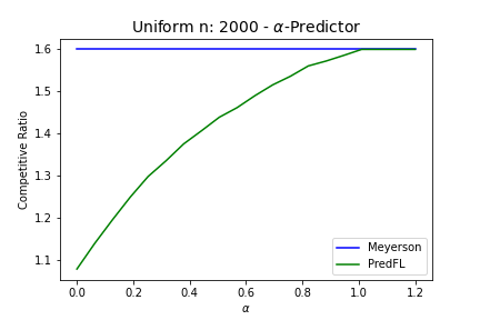
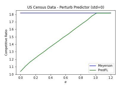
In Figure 6, we evaluate the performance of the algorithms for the parameter $\alpha$, introduced in the proof of Theorem 4.1. Generally, we observe a similar behavior on all three datasets. Specifically, our algorithm’s competitive ratio converges smoothly to that of Meyerson’s algorithm as the parameter $\alpha$ increases from $0$ to $1$.

Figure 6: A comparison of PredFL’s and Meyerson’s competitive ratio for different predictors and errors.

B.2 Standard Deviation

In Figure 7, each plot consists of three curves corresponding to a different standard deviation in the prediction accuracy. Namely, for each combination of $(\alpha,std)$, we sample, for each demand point $x$, a value $g_{\alpha}$ from the normal distribution $\mathcal{N}(\alpha,std)$ and give a prediction at distance $g_{\alpha}\cdot d(x,c^{\ast})$ to the optimal center $c^{\ast}$ where $x$ is connected to. Negative (resp. greater than $1$) values of $g_{\alpha}$ are replaced with $0$ (resp. $1$), thus ensuring that each prediction is always located between the optimal center $c^{\ast}$ and the demand location $x$.

As explained in Section 5, we observe that the competitive ratio is slightly decreasing with the standard deviation for both predictors alpha_gaussian_predictor, perturb_gaussian_predictor.

Figure 7: A comparison of PredFL’s and Meyerson’s competitive ratio for different values of the standard deviation of the prediction accuracy $\alpha$.

B.3 Random Reflections

In Figure 8, we evaluate the competitive ratio of our algorithm using two new methods for generating predictions, random_alpha_predictor, random_perturb_predictor. In both methods, for each new demand $x$ connected to an optimal center $c^{\ast}$, the prediction is at distance $\alpha\cdot d(x,c^{\ast})$ to $c^{\ast}$, where $\alpha$ is defined as in Theorem 4.1. However, each prediction is reflected randomly over all possible perpendicular hyperplanes passing through $c^{\ast}$. This is implemented by multiplying the vector $(\vec{x}-\vec{c}^{\ast})$, connecting the demand’s location $\vec{x}$ to the center’s location $\vec{c}^{\ast}$, with a random vector $\pm 1$ vector of the same dimension as that of $\vec{x}$ and $\vec{c}^{\ast}$. The prediction is obtained by adding the resulting vector to $\vec{c}^{\ast}$.

Interestingly, we observe that in all datasets, the competitive ratio of our algorithm reaches that of Meyerson’s algorithm, when the parameter $\alpha$ is close to $0.5$. This is because the random reflections might produce a prediction with distance to the nearest open facility significantly larger than the distance of the unreflected prediction to the nearest facility. Therefore, due to our facility opening rule, these predictions are more likely to open a new facility, resulting to an increased competitive ratio. Fortunately, this can only increase the competitive ratio by, at most, a constant factor.

Figure 8: A comparison of PredFL’s and Meyerson’s competitive ratio for random reflections.

References

- [1] Shaofeng H.-C. Jiang, Erzhi Liu, You Lyu, Zhihao Gavin Tang, and Yubo Zhang. Online facility location with predictions. In The Tenth International Conference on Learning Representations, ICLR 2022, Virtual Event, April 25-29, 2022. OpenReview.net, 2022.
- [2] Matteo Almanza, Flavio Chierichetti, Silvio Lattanzi, Alessandro Panconesi, and Giuseppe Re. Online facility location with multiple advice. In Marc’Aurelio Ranzato, Alina Beygelzimer, Yann N. Dauphin, Percy Liang, and Jennifer Wortman Vaughan, editors, Advances in Neural Information Processing Systems 34: Annual Conference on Neural Information Processing Systems 2021, NeurIPS 2021, December 6-14, 2021, virtual, pages 4661–4673, 2021.
- [3] Andres Muñoz Medina and Sergei Vassilvitskii. Revenue optimization with approximate bid predictions. In Advances in Neural Information Processing Systems 30: Annual Conference on Neural Information Processing Systems 2017, 4-9 December 2017, Long Beach, CA, USA, pages 1858–1866, 2017.
- [4] Thodoris Lykouris and Sergei Vassilvitskii. Competitive caching with machine learned advice. In Proceedings of the 35th International Conference on Machine Learning, ICML 2018, Stockholmsmässan, Stockholm, Sweden, July 10-15, 2018, pages 3302–3311, 2018.
- [5] Allan Borodin and Ran El-Yaniv. Online computation and competitive analysis. Cambridge University Press, 1998.
- [6] Antonios Antoniadis, Themis Gouleakis, Pieter Kleer, and Pavel Kolev. Secretary and online matching problems with machine learned advice. CoRR, abs/2006.01026, 2020.
- [7] Manish Purohit, Zoya Svitkina, and Ravi Kumar. Improving online algorithms via ML predictions. In Advances in Neural Information Processing Systems 31: Annual Conference on Neural Information Processing Systems 2018, NeurIPS 2018, 3-8 December 2018, Montréal, Canada, pages 9684–9693, 2018.
- [8] Adam Meyerson. Online facility location. In 42nd Annual Symposium on Foundations of Computer Science, FOCS 2001, 14-17 October 2001, Las Vegas, Nevada, USA, pages 426–431. IEEE Computer Society, 2001.
- [9] Antonios Antoniadis, Christian Coester, Marek Eliás, Adam Polak, and Bertrand Simon. Online metric algorithms with untrusted predictions. In Proceedings of the 37th International Conference on Machine Learning, ICML 2020, 13-18 July 2020, Virtual Event, volume 119 of Proceedings of Machine Learning Research, pages 345–355. PMLR, 2020.
- [10] Sreenivas Gollapudi and Debmalya Panigrahi. Online algorithms for rent-or-buy with expert advice. In Proceedings of the 36th International Conference on Machine Learning, ICML 2019, 9-15 June 2019, Long Beach, California, USA, pages 2319–2327, 2019.
- [11] Shufan Wang, Jian Li, and Shiqiang Wang. Online algorithms for multi-shop ski rental with machine learned advice. In Hugo Larochelle, Marc’Aurelio Ranzato, Raia Hadsell, Maria-Florina Balcan, and Hsuan-Tien Lin, editors, Advances in Neural Information Processing Systems 33: Annual Conference on Neural Information Processing Systems 2020, NeurIPS 2020, December 6-12, 2020, virtual, 2020.
- [12] Amos Fiat, Richard M. Karp, Michael Luby, Lyle A. McGeoch, Daniel Dominic Sleator, and Neal E. Young. Competitive paging algorithms. J. Algorithms, 12(4):685–699, 1991.
- [13] Dhruv Rohatgi. Near-optimal bounds for online caching with machine learned advice. In Proceedings of the 2020 ACM-SIAM Symposium on Discrete Algorithms, SODA 2020, Salt Lake City, UT, USA, January 5-8, 2020, pages 1834–1845, 2020.
- [14] Alexander Wei. Better and simpler learning-augmented online caching. In Jaroslaw Byrka and Raghu Meka, editors, Approximation, Randomization, and Combinatorial Optimization. Algorithms and Techniques, APPROX/RANDOM 2020, August 17-19, 2020, Virtual Conference, volume 176 of LIPIcs, pages 60:1–60:17. Schloss Dagstuhl - Leibniz-Zentrum für Informatik, 2020.
- [15] Silvio Lattanzi, Thomas Lavastida, Benjamin Moseley, and Sergei Vassilvitskii. Online scheduling via learned weights. In Proceedings of the 2020 ACM-SIAM Symposium on Discrete Algorithms, SODA 2020, Salt Lake City, UT, USA, January 5-8, 2020, pages 1859–1877, 2020.
- [16] Étienne Bamas, Andreas Maggiori, Lars Rohwedder, and Ola Svensson. Learning augmented energy minimization via speed scaling. In Hugo Larochelle, Marc’Aurelio Ranzato, Raia Hadsell, Maria-Florina Balcan, and Hsuan-Tien Lin, editors, Advances in Neural Information Processing Systems 33: Annual Conference on Neural Information Processing Systems 2020, NeurIPS 2020, December 6-12, 2020, virtual, 2020.
- [17] Étienne Bamas, Andreas Maggiori, and Ola Svensson. The primal-dual method for learning augmented algorithms. In Hugo Larochelle, Marc’Aurelio Ranzato, Raia Hadsell, Maria-Florina Balcan, and Hsuan-Tien Lin, editors, Advances in Neural Information Processing Systems 33: Annual Conference on Neural Information Processing Systems 2020, NeurIPS 2020, December 6-12, 2020, virtual, 2020.
- [18] Michael Mitzenmacher. Scheduling with predictions and the price of misprediction. In Thomas Vidick, editor, 11th Innovations in Theoretical Computer Science Conference, ITCS 2020, January 12-14, 2020, Seattle, Washington, USA, volume 151 of LIPIcs, pages 14:1–14:18. Schloss Dagstuhl - Leibniz-Zentrum für Informatik, 2020.
- [19] Mohammad Mahdian, Hamid Nazerzadeh, and Amin Saberi. Online optimization with uncertain information. ACM Trans. Algorithms, 8(1):2:1–2:29, 2012.
- [20] R.L. Francis (Editors) P.B. Mirchandani. Discrete Location Theory. Willey, 1990.
- [21] Z. Drezner and H.W. Hamacher (Editors). Facility Location: Applications and Theory. Springer, 2004.
- [22] D. Shmoys. Approximation Algorithms for Facility Location Problems. In 3rd Workshop on Approximation Algorithms for Combinatorial Optimization, volume 1913 of LNCS, pages 27–33, 2000.
- [23] Dimitris Fotakis. On the competitive ratio for online facility location. Algorithmica, 50(1):1–57, 2008.
- [24] Dimitris Fotakis. A primal-dual algorithm for online non-uniform facility location. J. Discrete Algorithms, 5(1):141–148, 2007.
- [25] Aris Anagnostopoulos, Russell Bent, Eli Upfal, and Pascal Van Hentenryck. A simple and deterministic competitive algorithm for online facility location. Inf. Comput., 194(2):175–202, 2004.
- [26] Dimitris Fotakis. Online and incremental algorithms for facility location. SIGACT News, 42(1):97–131, 2011.
- [27] Marek Cygan, Artur Czumaj, Marcin Mucha, and Piotr Sankowski. Online facility location with deletions. In Yossi Azar, Hannah Bast, and Grzegorz Herman, editors, 26th Annual European Symposium on Algorithms, ESA 2018, August 20-22, 2018, Helsinki, Finland, volume 112 of LIPIcs, pages 21:1–21:15. Schloss Dagstuhl - Leibniz-Zentrum für Informatik, 2018.
- [28] Vincent Cohen-Addad, Niklas Hjuler, Nikos Parotsidis, David Saulpic, and Chris Schwiegelshohn. Fully dynamic consistent facility location. In Hanna M. Wallach, Hugo Larochelle, Alina Beygelzimer, Florence d’Alché-Buc, Emily B. Fox, and Roman Garnett, editors, Advances in Neural Information Processing Systems 32: Annual Conference on Neural Information Processing Systems 2019, NeurIPS 2019, December 8-14, 2019, Vancouver, BC, Canada, pages 3250–3260, 2019.
- [29] Xiangyu Guo, Janardhan Kulkarni, Shi Li, and Jiayi Xian. On the facility location problem in online and dynamic models. In Jaroslaw Byrka and Raghu Meka, editors, Approximation, Randomization, and Combinatorial Optimization. Algorithms and Techniques, APPROX/RANDOM 2020, August 17-19, 2020, Virtual Conference, volume 176 of LIPIcs, pages 42:1–42:23. Schloss Dagstuhl - Leibniz-Zentrum für Informatik, 2020.
- [30] Abdolhossein Hoorfar and Mehdi Hassani. Inequalities on the lambert w function and hyperpower function. J. Inequal. Pure and Appl. Math, 9(2):5–9, 2008.
- [31] Andrew Chi-Chih Yao. Probabilistic computations: Toward a unified measure of complexity (extended abstract). In 18th Annual Symposium on Foundations of Computer Science, Providence, Rhode Island, USA, 31 October - 1 November 1977, pages 222–227. IEEE Computer Society, 1977.
- [32] J. A. Blackard, D. J. Dean, and C. W. Anderson. Covertype data set. https://archive.ics.uci.edu/ml/datasets/covertype.
- [33] C. Meek, B. Thiesson, and D. Heckerman. Us census data, 1990. http://archive.ics.uci.edu/ml/datasets/US+Census+Data+(1990).