A lower bound for the spectral gap of the conjugate Kac process with 3 interacting particles

Luís Simão Ferreira Supported by CMAF-CIO grant UIDP/04561/2020.
Abstract

In this paper, we proceed as suggested in the final section of [2] and prove a lower bound for the spectral gap of the conjugate Kac process with 3 interacting particles. This bound turns out to be around 0.020.020.02, which is already physically meaningful, and we perform Monte Carlo simulations to provide a better empirical estimate for this value via entropy production inequalities. This finishes a complete quantitative estimate of the spectral gap of the Kac process.

Acknowledgements

The author would like to thank CMAF-CIO for the opportunity to develop this work and professor José Francisco Rodrigues for bringing this topic to my attention.

I also would like to extend my deepest gratitude to professor Eric Carlen, my supervisor, for all the patience, clear and intuitive explanations and everything that I have learned regarding functional analysis and mathematical physics for the duration of this project.

1 Introduction

N𝑁N-particle systems have been a target of flourishing research for the better part of the last 50 years, in particular due to their connection to classical statistical physics PDE’s via hydrodynamic limits. Thoroughly inspecting these collision processes allows us to better understand limiting cases such as the Boltzmann equation, while avoiding dealing with the equation explicitly, since it involves strong non-linearity.

In 1956, Marc Kac [1] introduced what we refer to as the Kac process, a reversible Markov process for N𝑁N spatially homogeneous particles with one dimensional velocities, which describes the evolution of the system as particles randomly collide in a momentum and energy conserving fashion.

A behaviour exhibited in many naturally occurring particle systems, and a desirable property of these models, is that of exponential decay to equilibrium. The easiest way one can prove such property is by showing the existence of a spectral gap for the generator of the process, and a uniform bound lets us draw conclusions as the number of particles becomes infinite. Recall that the spectral gap of an operator is defined as the infimum of its positive spectrum, which may coincide with the lowest non-zero eigenvalue, if these exist.

In essence, under the Kac process, if L𝐿L is the infinitesimal generator and f0subscript𝑓0f_{0} is an initial distribution in our state space, then it evolves as ft=etLf0subscript𝑓𝑡superscript𝑒𝑡𝐿subscript𝑓0f_{t}=e^{tL}f_{0}, and the existence of a spectral gap ΔΔ\Delta implies an exponential decay with rate at least equal to ΔΔ\Delta.

It is hard to relate relaxation in the N𝑁N-particle system to relaxation in the limit equation, unless one has uniform bounds on the spectral gap, independent of N𝑁N. Kac conjectured this to be true in his toy model, and this was successfuly proven later by Janvresse [5], but with one dimensional velocities and uniform jump rates, which nevertheless allows us to efficiently generate uniform points on the n𝑛n-sphere.

In a series of papers, Carlen, Carvalho and Loss [2] managed to prove the existence of a spectral gap for a one parameter family of Kac processes in 3-dimensions, undergoing more general collisions with rates that are not bounded away from zero. We will explore next the background of these papers.

1.1 The Kac process

More precisely, consider an additional physical parameter 0α20𝛼20\leq\alpha\leq 2 and an N𝑁N-tuple of velocities vjsubscript𝑣𝑗v_{j} in 3superscript3{{\mathbb{R}}}^{3} such that

1Nj=1Nvj=0,1Nj=1N|vj|2=1,formulae-sequence1𝑁superscriptsubscript𝑗1𝑁subscript𝑣𝑗01𝑁superscriptsubscript𝑗1𝑁superscriptsubscript𝑣𝑗21\frac{1}{N}\sum_{j=1}^{N}v_{j}=0,\frac{1}{N}\sum_{j=1}^{N}|v_{j}|^{2}=1, (1)

meaning that the total momentum is zero and the average kinetic energy per particle (with mass 2) is 1. These constraints describe our state space 𝒮Nsubscript𝒮𝑁\mathcal{S}_{N}, isometric to a sphere with 3N43𝑁43N-4 dimensions and radius N𝑁\sqrt{N}.

Before we move on, it is important to fix some notation. We will refer to elements of this state space 𝒮Nsubscript𝒮𝑁\mathcal{S}_{N} as a single letter v𝑣v, y𝑦y, and sometimes as a vector v𝑣\vec{v}, y𝑦\vec{y}, if it’s not clear from context. Letters with subscripts such as vjsubscript𝑣𝑗v_{j} shall always denote velocities in 3superscript3{{\mathbb{R}}}^{3}.

When the process begins, there is an associated exponential clock Ti,jsubscript𝑇𝑖𝑗T_{i,j} for each pair of velocities (vi,vj)subscript𝑣𝑖subscript𝑣𝑗(v_{i},v_{j}), with parameter

λi,j=N(N2)1|vivj|α,subscript𝜆𝑖𝑗𝑁superscriptbinomial𝑁21superscriptsubscript𝑣𝑖subscript𝑣𝑗𝛼\lambda_{i,j}=N\binom{N}{2}^{-1}|v_{i}-v_{j}|^{\alpha}, (2)

and the minimum

T:=mini,jTi,jassign𝑇subscript𝑖𝑗subscript𝑇𝑖𝑗T:=\min_{i,j}T_{i,j} (3)

yields our first collision time (and colliding pair). Given the restrictions above, these collisions can be parametrized in terms of a vector σ𝕊2𝜎superscript𝕊2\sigma\in\mathbb{S}^{2}:

vi(σ)superscriptsubscript𝑣𝑖𝜎\displaystyle v_{i}^{*}(\sigma) =vi+vj2+|vivj|2σ,absentsubscript𝑣𝑖subscript𝑣𝑗2subscript𝑣𝑖subscript𝑣𝑗2𝜎\displaystyle=\frac{v_{i}+v_{j}}{2}+\frac{|v_{i}-v_{j}|}{2}\sigma, (4)
vj(σ)superscriptsubscript𝑣𝑗𝜎\displaystyle v_{j}^{*}(\sigma) =vi+vj2|vivj|2σ.absentsubscript𝑣𝑖subscript𝑣𝑗2subscript𝑣𝑖subscript𝑣𝑗2𝜎\displaystyle=\frac{v_{i}+v_{j}}{2}-\frac{|v_{i}-v_{j}|}{2}\sigma. (5)

Another source of randomness on the system is then the determination of this direction vector σ𝜎\sigma. The particular choice we follow is uniform sampling, as it turns out to be more physically relevant, even though other distributions or rules could be used.

The cases 0α10𝛼10\leq\alpha\leq 1, with 0 being the Maxwellian molecule case and 1 the hard sphere case, are the ones of physical interest, but it turns out, as shown by Villani (regarding entropy production inequalities) [6] and as seen in the work of Carlen, Carvalho and Loss, that the ”super hard sphere” α=2𝛼2\alpha=2 case provides powerful insights for lower values of the parameter, and will later be our main focus.

Their proof is based on chaos estimates that quantify the ”near independence” of a finite set of coordinates. If σNsubscript𝜎𝑁\sigma_{N} denotes the uniform measure on the sphere 𝕊N(N)superscript𝕊𝑁𝑁\mathbb{S}^{N}(\sqrt{N}) with radius N𝑁\sqrt{N}, it is known that

limN+𝕊N(N)ϕ(v1,,vk)𝑑σN=kϕ(v1,,vk)𝑑γk,subscript𝑁subscriptsuperscript𝕊𝑁𝑁italic-ϕsubscript𝑣1subscript𝑣𝑘differential-dsubscript𝜎𝑁subscriptsuperscript𝑘italic-ϕsubscript𝑣1subscript𝑣𝑘differential-dsuperscript𝛾tensor-productabsent𝑘\lim_{N\to+\infty}\int_{\mathbb{S}^{N}(\sqrt{N})}\phi(v_{1},...,v_{k})d\sigma_{N}=\int_{{{\mathbb{R}}}^{k}}\phi(v_{1},...,v_{k})d\gamma^{\otimes k}, (6)

with γ𝛾\gamma being the Gaussian measure in {{\mathbb{R}}}, and we say that the measure σNsubscript𝜎𝑁\sigma_{N} is γ𝛾\gamma-chaotic. In general, if the above equality holds for μ𝜇\mu and a sequence of measures μNsubscript𝜇𝑁\mu_{N}, μNsubscript𝜇𝑁\mu_{N} is said to be μ𝜇\mu-chaotic.

Another important step of the proof is the introduction of a conjugate process, which allows for a clever induction argument. With the right choice of coordinates, integrals over the state space can be factored as

𝒮Nϕ(v)𝑑σN=B[SN1ϕ(Tj(y,v))𝑑σN1]𝑑νN(v),subscriptsubscript𝒮𝑁italic-ϕ𝑣differential-dsubscript𝜎𝑁subscript𝐵delimited-[]subscriptsubscript𝑆𝑁1italic-ϕsubscript𝑇𝑗𝑦𝑣differential-dsubscript𝜎𝑁1differential-dsubscript𝜈𝑁𝑣\int_{\mathcal{S}_{N}}\phi(\vec{v})d\sigma_{N}=\int_{B}\bigg{[}\int_{S_{N-1}}\phi(T_{j}(\vec{y},v))d\sigma_{N-1}\bigg{]}d\nu_{N}(v), (7)

with B𝐵B the unit ball in 3superscript3{{\mathbb{R}}}^{3}. T1:𝒮N1×B𝒮N:subscript𝑇1subscript𝒮𝑁1𝐵subscript𝒮𝑁T_{1}:\mathcal{S}_{N-1}\times B\to\mathcal{S}_{N} is given by

T1(y,v)=(N1v,β(v)y11N1v,,β(v)yN11N1v),subscript𝑇1𝑦𝑣𝑁1𝑣𝛽𝑣subscript𝑦11𝑁1𝑣𝛽𝑣subscript𝑦𝑁11𝑁1𝑣T_{1}(y,v)=\bigg{(}\sqrt{N-1}v,\beta(v)y_{1}-\frac{1}{\sqrt{N-1}}v,...,\beta(v)y_{N-1}-\frac{1}{\sqrt{N-1}}v\bigg{)}, (8)

while Tjsubscript𝑇𝑗T_{j} is defined analogously but with v𝑣v going to the j𝑗j-th coordinate, and

β2(v):=NN1(1|v|2).assignsuperscript𝛽2𝑣𝑁𝑁11superscript𝑣2\beta^{2}(v):=\frac{N}{N-1}(1-|v|^{2}). (9)

Finally, the measure νNsubscript𝜈𝑁\nu_{N} on B𝐵B is defined as

dνN(v)=|𝕊3N7||𝕊3N4|(1|v|2)(3N8)/2dv,𝑑subscript𝜈𝑁𝑣superscript𝕊3𝑁7superscript𝕊3𝑁4superscript1superscript𝑣23𝑁82𝑑𝑣d\nu_{N}(v)=\frac{|\mathbb{S}^{3N-7}|}{|\mathbb{S}^{3N-4}|}(1-|v|^{2})^{(3N-8)/2}dv, (10)

which is what we refer to as the equilibrium radial measure, as it is the radial marginal of the velocities for the uniform measure in 𝒮Nsubscript𝒮𝑁\mathcal{S}_{N}.

As we will verify later, this formula allows for an inductive inequality of the type

ΔN,αNN1ΔN1,αΔ^N,α,subscriptΔ𝑁𝛼𝑁𝑁1subscriptΔ𝑁1𝛼subscript^Δ𝑁𝛼\Delta_{N,\alpha}\geq\frac{N}{N-1}\Delta_{N-1,\alpha}\hat{\Delta}_{N,\alpha}, (11)

where Δ^N,αsubscript^Δ𝑁𝛼\hat{\Delta}_{N,\alpha} is the spectral gap of a conjugate Kac process, with vastly simplified dynamics. Furthermore, the authors make use of this fact to prove that there are K0>0subscript𝐾00K_{0}>0 and N0subscript𝑁0N_{0}\in{{\mathbb{N}}} such that

ΔN,αK0ΔN0,α>0,subscriptΔ𝑁𝛼subscript𝐾0subscriptΔsubscript𝑁0𝛼0\Delta_{N,\alpha}\geq K_{0}\Delta_{N_{0},\alpha}>0, (12)

leaving only the base case to show. For N=2𝑁2N=2, the process is trivial, as the constraints completely determine one velocity from the other. Finally, making use of a compactness argument to show that Δ^3,α>0subscript^Δ3𝛼0\hat{\Delta}_{3,\alpha}>0, it follows that

Δ3,α32Δ2,αΔ^3,α>0.subscriptΔ3𝛼32subscriptΔ2𝛼subscript^Δ3𝛼0\Delta_{3,\alpha}\geq\frac{3}{2}\Delta_{2,\alpha}\hat{\Delta}_{3,\alpha}>0. (13)

However, unlike previous bounds that could be explicitly computed, this does not give any quantitative information about Δ^3,αsubscript^Δ3𝛼\hat{\Delta}_{3,\alpha}, besides positivity, and it remains to be shown that this gap is physically meaningful when interpreted as an expected relaxation time. In this paper, we compute a lower bound for the spectral gap of the conjugate Kac process with 3 particles.

Even though the proof provided in [2] makes use of asymptotic methods in the form of quantitative chaos estimates, the results are strong enough to hold already for all N4𝑁4N\geq 4, and provide a positive gap. This fails for N=3𝑁3N=3.

Due to the fact that N=2𝑁2N=2 is already trivial, and most methods allow for good estimates for N>3𝑁3N>3, one would expect this case to be accessible. Unfortunately, this is not true, as most methods fail to provide a positive gap in this number of dimensions.

1.2 Structure of the paper

This paper is organized as follows.

In section 2, we introduce our main object of study, the conjugate Kac process, building up the necessary tools and finally stating our main result. We also explore the possibility of obtaining spectral gap bounds via entropy production inequalities and, while not being able to prove it analytically, present some numerical evidence of such results.

The proof is developed over section 3. We begin by inspecting the spectrum of our main tool, the correlation operator K𝐾K, and proving suitable upper bounds on the eigenvalue sequence κn,subscript𝜅𝑛\kappa_{n,\ell}.

The proof itself is then broken down over the anti-symmetric and symmetric sectors, as they are orthogonal to each other. The first one is handled fairly quickly, while the symmetric sector, which is of bigger physical interest due to its relation to the limit equation, requires a more hands-on approach. We treat different angular momentum sectors, where different methods handle ’large’ and ’small’ values of \ell, leaving only a finite amount of eigenvalues to be computed.

2 The conjugate Kac process

We will now define the family of reversible Markov jump processes on 𝒮Nsubscript𝒮𝑁\mathcal{S}_{N}, conjugate to the Kac process. Fixing a number of interacting particles N𝑁N, 0<α20𝛼20<\alpha\leq 2, and given vSN𝑣subscript𝑆𝑁\vec{v}\in S_{N}, let {T^1,,T^N}subscript^𝑇1subscript^𝑇𝑁\{\hat{T}_{1},...,\hat{T}_{N}\} be a set of N𝑁N independent exponential variables with parameter λk(v)subscript𝜆𝑘𝑣\lambda_{k}(\vec{v}) of T^ksubscript^𝑇𝑘\hat{T}_{k} given by

λk(v)=1N[N2(1+|vk|2)N(N1)2]α/2.subscript𝜆𝑘𝑣1𝑁superscriptdelimited-[]superscript𝑁21superscriptsubscript𝑣𝑘2𝑁superscript𝑁12𝛼2\lambda_{k}(\vec{v})=\frac{1}{N}\bigg{[}\frac{N^{2}-(1+|v_{k}|^{2})N}{(N-1)^{2}}\bigg{]}^{\alpha/2}. (14)

Due to the restraints on energy and momentum, the maximum of |vk|2superscriptsubscript𝑣𝑘2|v_{k}|^{2} is N1𝑁1N-1, and thus the parameter is always positive.

Let T^=min{T^1,,T^N}^𝑇subscript^𝑇1subscript^𝑇𝑁\hat{T}=\min\{\hat{T}_{1},...,\hat{T}_{N}\} be the first jump time, and let k𝑘k be the corresponding index. At this time, the process makes a conditional jump to uniform to a new point vSN𝑣subscript𝑆𝑁\vec{v}\in S_{N}, fixing vksubscript𝑣𝑘v_{k}, and all other velocities are re-sampled uniformly, conditional on vksubscript𝑣𝑘v_{k}. Even though this process is trivial for N=2𝑁2N=2, since the momentum equation completely determines one velocity from the other, our N=3𝑁3N=3 case is subtle.

The generator of this process can be obtained via projection (or conditional expectation) operators. Recall that, for any ϕL2(σN)italic-ϕsuperscript𝐿2subscript𝜎𝑁\phi\in L^{2}(\sigma_{N}), there is a unique element f(vk)𝑓subscript𝑣𝑘f(v_{k}) of L2(σN)superscript𝐿2subscript𝜎𝑁L^{2}(\sigma_{N}) such that

SNϕ(v)g(vk)𝑑σN=SNf(vk)g(vk)𝑑σN,subscriptsubscript𝑆𝑁italic-ϕ𝑣𝑔subscript𝑣𝑘differential-dsubscript𝜎𝑁subscriptsubscript𝑆𝑁𝑓subscript𝑣𝑘𝑔subscript𝑣𝑘differential-dsubscript𝜎𝑁\int_{S_{N}}\phi(\vec{v})g(v_{k})d\sigma_{N}=\int_{S_{N}}f(v_{k})g(v_{k})d\sigma_{N}, (15)

and we define this way the conditional expectation of ϕitalic-ϕ\phi, given vksubscript𝑣𝑘v_{k}:

Pkϕ:=𝔼[ϕ|vk].assignsubscript𝑃𝑘italic-ϕ𝔼delimited-[]conditionalitalic-ϕsubscript𝑣𝑘P_{k}\phi:={{\mathbb{E}}}[\phi|v_{k}]. (16)

This can also be understood as an orthogonal projection onto the subspace of square integrable functions that depend only on the k𝑘k-th coordinate. Furthermore, the factorization formula (7) gives us an expression for this operator:

Pkϕ(v)=𝒮N1ϕ(Tk(y,vk/N1)dσN1.P_{k}\phi(v)=\int_{\mathcal{S}_{N-1}}\phi(T_{k}(y,v_{k}/\sqrt{N-1})d\sigma_{N-1}. (17)

The generator of this process can then be written as

L^N,αf=1Nk=1N1N[N2(1+|vk|2)N(N1)2]α/2[fPkf],subscript^𝐿𝑁𝛼𝑓1𝑁superscriptsubscript𝑘1𝑁1𝑁superscriptdelimited-[]superscript𝑁21superscriptsubscript𝑣𝑘2𝑁superscript𝑁12𝛼2delimited-[]𝑓subscript𝑃𝑘𝑓\hat{L}_{N,\alpha}f=-\frac{1}{N}\sum_{k=1}^{N}\frac{1}{N}\bigg{[}\frac{N^{2}-(1+|v_{k}|^{2})N}{(N-1)^{2}}\bigg{]}^{\alpha/2}[f-P_{k}f], (18)

and it is also useful to define

wN(vk):=N2(1+|vk|2)N(N1)2.assignsubscript𝑤𝑁subscript𝑣𝑘superscript𝑁21superscriptsubscript𝑣𝑘2𝑁superscript𝑁12w_{N}(v_{k}):=\frac{N^{2}-(1+|v_{k}|^{2})N}{(N-1)^{2}}. (19)

It is easy to prove self-adjointness, as we would expect from the reversibility of the process, and its null space is spanned by the constants. Similarly as before, the spectral gap of the conjugate Kac process is defined as

Δ^N,α:=inf{𝒟N,α(f,f)|f,1L2(σN),fL2(σN)2=1},assignsubscript^Δ𝑁𝛼infimumconditional-setsubscript𝒟𝑁𝛼𝑓𝑓subscript𝑓1superscript𝐿2subscript𝜎𝑁subscriptsuperscriptnorm𝑓2superscript𝐿2subscript𝜎𝑁1\hat{\Delta}_{N,\alpha}:=\inf\{\mathcal{D}_{N,\alpha}(f,f)|\langle f,1\rangle_{L^{2}(\sigma_{N})},\|f\|^{2}_{L^{2}(\sigma_{N})}=1\}, (20)

with

𝒟N,α(f,f)subscript𝒟𝑁𝛼𝑓𝑓\displaystyle\mathcal{D}_{N,\alpha}(f,f) :=f,L^N,αfL2(σN)assignabsentsubscript𝑓subscript^𝐿𝑁𝛼𝑓superscript𝐿2subscript𝜎𝑁\displaystyle:=-\langle f,\hat{L}_{N,\alpha}f\rangle_{L^{2}(\sigma_{N})}
=1Nk=1N1NSN[N2(1+|vk|2)N(N1)2]α/2[f2fPkf]𝑑σN.absent1𝑁superscriptsubscript𝑘1𝑁1𝑁subscriptsubscript𝑆𝑁superscriptdelimited-[]superscript𝑁21superscriptsubscript𝑣𝑘2𝑁superscript𝑁12𝛼2delimited-[]superscript𝑓2𝑓subscript𝑃𝑘𝑓differential-dsubscript𝜎𝑁\displaystyle=\frac{1}{N}\sum_{k=1}^{N}\frac{1}{N}\int_{S_{N}}\bigg{[}\frac{N^{2}-(1+|v_{k}|^{2})N}{(N-1)^{2}}\bigg{]}^{\alpha/2}[f^{2}-fP_{k}f]d\sigma_{N}. (21)

We are at this moment in conditions of explaining how this process arises. Let LN,αsubscript𝐿𝑁𝛼L_{N,\alpha} be the infinitesimal generator of the Kac process,

N,α(f,f)=f,LN,αfsubscript𝑁𝛼𝑓𝑓𝑓subscript𝐿𝑁𝛼𝑓\mathcal{E}_{N,\alpha}(f,f)=-\langle f,L_{N,\alpha}f\rangle (22)

the Dirichlet form associated with LN,αsubscript𝐿𝑁𝛼L_{N,\alpha} and N,α(f,f|vk)subscript𝑁𝛼𝑓conditional𝑓subscript𝑣𝑘\mathcal{E}_{N,\alpha}(f,f|v_{k}) the conditional Dirichlet form obtained by factorizing, so that

N,α(f,f)=NN1(1Nk=1NBwNα/2(vk)N,α(f,f|vk)𝑑νN(vk/N1)).subscript𝑁𝛼𝑓𝑓𝑁𝑁11𝑁superscriptsubscript𝑘1𝑁subscript𝐵superscriptsubscript𝑤𝑁𝛼2subscript𝑣𝑘subscript𝑁𝛼𝑓conditional𝑓subscript𝑣𝑘differential-dsubscript𝜈𝑁subscript𝑣𝑘𝑁1\mathcal{E}_{N,\alpha}(f,f)=\frac{N}{N-1}\bigg{(}\frac{1}{N}\sum_{k=1}^{N}\int_{B}w_{N}^{\alpha/2}(v_{k})\mathcal{E}_{N,\alpha}(f,f|v_{k})d\nu_{N}(v_{k}/\sqrt{N-1})\bigg{)}. (23)

Then, using the spectral gap for N1𝑁1N-1 particles, one has

N,α(f,f)NN1ΔN1,α(1Nk=1N𝒮NwNα/2(vk)[fPkf]2𝑑σN),subscript𝑁𝛼𝑓𝑓𝑁𝑁1subscriptΔ𝑁1𝛼1𝑁superscriptsubscript𝑘1𝑁subscriptsubscript𝒮𝑁superscriptsubscript𝑤𝑁𝛼2subscript𝑣𝑘superscriptdelimited-[]𝑓subscript𝑃𝑘𝑓2differential-dsubscript𝜎𝑁\mathcal{E}_{N,\alpha}(f,f)\geq\frac{N}{N-1}\Delta_{N-1,\alpha}\bigg{(}\frac{1}{N}\sum_{k=1}^{N}\int_{\mathcal{S}_{N}}w_{N}^{\alpha/2}(v_{k})[f-P_{k}f]^{2}d\sigma_{N}\bigg{)}, (24)

and the quantity in brackets corresponds exactly to (2).

Now, define the self-adjoint operators

W(α)=W(α)(v):=1Nk=1NwNα/2(vk)superscript𝑊𝛼superscript𝑊𝛼𝑣assign1𝑁superscriptsubscript𝑘1𝑁superscriptsubscript𝑤𝑁𝛼2subscript𝑣𝑘W^{(\alpha)}=W^{(\alpha)}(v):=\frac{1}{N}\sum_{k=1}^{N}w_{N}^{\alpha/2}(v_{k}) (25)

and

P(α)=1Nk=1NwNα/2(vk)Pk,superscript𝑃𝛼1𝑁superscriptsubscript𝑘1𝑁superscriptsubscript𝑤𝑁𝛼2subscript𝑣𝑘subscript𝑃𝑘P^{(\alpha)}=\frac{1}{N}\sum_{k=1}^{N}w_{N}^{\alpha/2}(v_{k})P_{k}, (26)

an average of weighted projections, so that we have L^N,α=W(α)P(α)subscript^𝐿𝑁𝛼superscript𝑊𝛼superscript𝑃𝛼\hat{L}_{N,\alpha}=W^{(\alpha)}-P^{(\alpha)}. For α=2𝛼2\alpha=2 and N=3𝑁3N=3, we see that W(2)=34superscript𝑊234W^{(2)}=\frac{3}{4}, and (20) becomes

Δ^3,2=34μ3,subscript^Δ3234subscript𝜇3\hat{\Delta}_{3,2}=\frac{3}{4}-\mu_{3}, (27)

with

μ3:=sup{f,P(2)fL2(dσ3)|fL2(dσ3)=1,f,1L2(dσ3)=0}.assignsubscript𝜇3supremumconditional-setsubscript𝑓superscript𝑃2𝑓superscript𝐿2𝑑subscript𝜎3formulae-sequencesubscriptnorm𝑓superscript𝐿2𝑑subscript𝜎31subscript𝑓1superscript𝐿2𝑑subscript𝜎30\mu_{3}:=\sup\{\langle f,P^{(2)}f\rangle_{L^{2}(d\sigma_{3})}|\|f\|_{L^{2}(d\sigma_{3})}=1,\langle f,1\rangle_{L^{2}(d\sigma_{3})}=0\}. (28)

The spectrum of P(α)superscript𝑃𝛼P^{(\alpha)} is also studied on [3]. More importantly, for α=2𝛼2\alpha=2, the following is true

Lemma 2.1

The essential spectrum of P(2)superscript𝑃2P^{(2)} is the interval [0,12]012[0,\frac{1}{2}], and the remaining spectrum can only consist of isolated eigenvalues in (12,34)1234\big{(}\frac{1}{2},\frac{3}{4}\big{)}.

Note that, in particular, 3434\frac{3}{4} cannot be an accumulation point, and thus this proves that the spectral gap exists. Moreover, if μ312subscript𝜇312\mu_{3}\leq\frac{1}{2}, we immediately have that Δ^3,20.25subscript^Δ320.25\hat{\Delta}_{3,2}\geq 0.25, and if 12<μ3<3412subscript𝜇334\frac{1}{2}<\mu_{3}<\frac{3}{4}, it is an eigenvalue of P(2)superscript𝑃2P^{(2)}.

We then turn to the eigenvalue equation P(2)f=λfsuperscript𝑃2𝑓𝜆𝑓P^{(2)}f=\lambda f to obtain the only missing estimate for a fully quantitative result on the three particle spectral gap Δ^3,2subscript^Δ32\hat{\Delta}_{3,2}. In [2], the authors break this down to the symmetric and anti-symmetric eigen-sectors, as they are mutually orthogonal. A computation for the anti-symmetric case is provided, and a suggestion is made on how to proceed for the remaining case. In section 3.2 we explain and slightly improve the former, while the latter is treated in section 3.3 - this last case proved to be much harder, due to the analytical difficulties in dealing with the spectrum of the conditional expectation operator (see section 3.1).

Using this method, we were able to prove the following main result:

Theorem 2.1

The spectral gap of the conjugate Kac process in 3 dimensions, with α=2𝛼2\alpha=2, is at least 0.019840.019840.01984.

The actual computations we provide show a result slightly less then 0.020.020.02 in order to simplify and reduce the amount of cases, but could easily be adapted to achieve this quantity at the expense of explicitly determining a larger number of eigenvalues. Note that it is expected that the true value of the gap is larger, and we will illustrate this next.

2.1 Spectral gap bounds via entropy production inequalities

Cedric Villani [6] was the first to prove entropy production inequalities for variants of the Kac process, namely with one dimensional velocities. Even though obtaining such bounds for the 3-dimensional Kac process is still an open problem, one can adopt a similar reasoning and attempt to derive entropy production inequalities for the simpler conjugate process. Recall that the entropy functional of a suitable density f𝑓f on 𝒮Nsubscript𝒮𝑁\mathcal{S}_{N} is defined as

H(f):=𝒮NflogfdσN,assign𝐻𝑓subscriptsubscript𝒮𝑁𝑓𝑓𝑑subscript𝜎𝑁H(f):=\int_{\mathcal{S}_{N}}f\log fd\sigma_{N}, (29)

and the entropy production of a process with generator L^N,αsubscript^𝐿𝑁𝛼\hat{L}_{N,\alpha} as

DL^N,α(f):=ddt(H(etL^N,αf))0,assignsubscript𝐷subscript^𝐿𝑁𝛼𝑓𝑑𝑑𝑡𝐻superscript𝑒𝑡subscript^𝐿𝑁𝛼𝑓0D_{\hat{L}_{N,\alpha}}(f):=-\frac{d}{dt}\bigg{(}H(e^{t\hat{L}_{N,\alpha}}f)\bigg{)}\geq 0, (30)

so that we can look for estimates of the type

DL^N,α(f)CN,αH(f),subscript𝐷subscript^𝐿𝑁𝛼𝑓subscript𝐶𝑁𝛼𝐻𝑓D_{\hat{L}_{N,\alpha}}(f)\geq C_{N,\alpha}H(f), (31)

with CN,αsubscript𝐶𝑁𝛼C_{N,\alpha} a constant independent of f𝑓f, and depending on L^N,αsubscript^𝐿𝑁𝛼\hat{L}_{N,\alpha} only via the parameters describing the process.

Results of the above type are stronger than spectral gap estimates, as a classical linearization procedure implies the latter. More precisely, taking f:=1+εhassign𝑓1𝜀f:=1+\varepsilon h, with ε>0𝜀0\varepsilon>0 and

𝒮Nh𝑑σN=0,subscriptsubscript𝒮𝑁differential-dsubscript𝜎𝑁0\int_{\mathcal{S}_{N}}hd\sigma_{N}=0,

and expanding in first order leads us to

Δ^N,α12CN,α.subscript^Δ𝑁𝛼12subscript𝐶𝑁𝛼\hat{\Delta}_{N,\alpha}\geq\frac{1}{2}C_{N,\alpha}. (32)

One advantage of the entropy production approach is that we can actually measure the empirical entropy in Monte Carlo simulations, and obtain an estimate of the true spectral gap by analyzing the log-entropy decay, which we will do next.

First, by symmetrizing one can compute the entropy production functional of the conjugate process:

DN,α(f):=1Nk=1N𝒮NwNα/2(vk)logf[fPkf]𝑑σN.assignsubscript𝐷𝑁𝛼𝑓1𝑁superscriptsubscript𝑘1𝑁subscriptsubscript𝒮𝑁superscriptsubscript𝑤𝑁𝛼2subscript𝑣𝑘𝑓delimited-[]𝑓subscript𝑃𝑘𝑓differential-dsubscript𝜎𝑁D_{N,\alpha}(f):=\frac{1}{N}\sum_{k=1}^{N}\int_{\mathcal{S}_{N}}w_{N}^{\alpha/2}(v_{k})\log f[f-P_{k}f]d\sigma_{N}. (33)

Specializing to α=2𝛼2\alpha=2, and using the convexity of logt𝑡-\log t and the fact that

1Nk=1NwN(v)=1,1𝑁superscriptsubscript𝑘1𝑁subscript𝑤𝑁𝑣1\frac{1}{N}\sum_{k=1}^{N}w_{N}(v)=1, (34)

we obtain

DN,2(f)D¯N,2(f):=subscript𝐷𝑁2𝑓subscript¯𝐷𝑁2𝑓assignabsent\displaystyle D_{N,2}(f)\geq\bar{D}_{N,2}(f):= 1Nk=1N𝒮NwN(vk)[flogfPkflogPkf]𝑑σN1𝑁superscriptsubscript𝑘1𝑁subscriptsubscript𝒮𝑁subscript𝑤𝑁subscript𝑣𝑘delimited-[]𝑓𝑓subscript𝑃𝑘𝑓subscript𝑃𝑘𝑓differential-dsubscript𝜎𝑁\displaystyle\frac{1}{N}\sum_{k=1}^{N}\int_{\mathcal{S}_{N}}w_{N}(v_{k})[f\log f-P_{k}f\log P_{k}f]d\sigma_{N} (35)
=\displaystyle= H(f)1Nk=1N𝒮NwN(vk)[PkflogPkfPkf+1]𝑑σN.𝐻𝑓1𝑁superscriptsubscript𝑘1𝑁subscriptsubscript𝒮𝑁subscript𝑤𝑁subscript𝑣𝑘delimited-[]subscript𝑃𝑘𝑓subscript𝑃𝑘𝑓subscript𝑃𝑘𝑓1differential-dsubscript𝜎𝑁\displaystyle H(f)-\frac{1}{N}\sum_{k=1}^{N}\int_{\mathcal{S}_{N}}w_{N}(v_{k})[P_{k}f\log P_{k}f-P_{k}f+1]d\sigma_{N}. (36)

Now, as tlogtt+10𝑡𝑡𝑡10t\log t-t+1\geq 0 for all t>0𝑡0t>0 and wN(v)NN1subscript𝑤𝑁𝑣𝑁𝑁1w_{N}(v)\leq\frac{N}{N-1} for all v𝑣v, we see that the k𝑘k-th summand in the second term is less than NN1H(Pkf)𝑁𝑁1𝐻subscript𝑃𝑘𝑓\frac{N}{N-1}H(P_{k}f), and thus we have

D¯N,2(f)H(f)1N1k=1NH(Pkf)subscript¯𝐷𝑁2𝑓𝐻𝑓1𝑁1superscriptsubscript𝑘1𝑁𝐻subscript𝑃𝑘𝑓\bar{D}_{N,2}(f)\geq H(f)-\frac{1}{N-1}\sum_{k=1}^{N}H(P_{k}f) (37)

To continue, we need to somehow relate the entropy of the marginals Pkfsubscript𝑃𝑘𝑓P_{k}f with the entropy of the joint distribution f𝑓f. Fortunately, this is precisely developed in [7] and [8], and we make use of the CCL inequality (in 3 dimensions),

N1Nk=1NH(Pkf)2H(f),𝑁1𝑁superscriptsubscript𝑘1𝑁𝐻subscript𝑃𝑘𝑓2𝐻𝑓\frac{N-1}{N}\sum_{k=1}^{N}H(P_{k}f)\leq 2H(f), (38)

thus giving us

D¯N,2(f)(12N(N1)2)H(f).subscript¯𝐷𝑁2𝑓12𝑁superscript𝑁12𝐻𝑓\bar{D}_{N,2}(f)\geq\bigg{(}1-\frac{2N}{(N-1)^{2}}\bigg{)}H(f). (39)

As for the much simpler case of α=0𝛼0\alpha=0 with constant jump rates, one can easily verify by slightly adapting the computations above that this yields

CN,0=N3N1.subscript𝐶𝑁0𝑁3𝑁1C_{N,0}=\frac{N-3}{N-1}. (40)

With this quick argument, we can then state the following:

Proposition 2.2

The entropy production functional of the Kac process in 3 dimensions, DN,αsubscript𝐷𝑁𝛼D_{N,\alpha}, satisfies

DN,2(f)(12N(N1)2)H(f),subscript𝐷𝑁2𝑓12𝑁superscript𝑁12𝐻𝑓D_{N,2}(f)\geq\bigg{(}1-\frac{2N}{(N-1)^{2}}\bigg{)}H(f), (41)

and

DN,0(f)N3N1H(f).subscript𝐷𝑁0𝑓𝑁3𝑁1𝐻𝑓D_{N,0}(f)\geq\frac{N-3}{N-1}H(f). (42)

Thus, for N4𝑁4N\geq 4, the spectral gap of the conjugate Kac process in 3 dimensions is at least 118118\frac{1}{18} for the super hard sphere case, and 1616\frac{1}{6} for the Maxwellian molecule case.

Sadly, this is not quite enough, and the bounds degenerate at N=3𝑁3N=3, and adapting Villani’s approach seems to give degenerate bounds at N=3𝑁3N=3 as well, even though the technique is much stronger than the one we use above. The main culprit seems to be the CCL inequality (38) as the extra N/(N1)𝑁𝑁1N/(N-1) factor, which isn’t present for the 1-dimensional case, loses us enough for the method to fail.

This makes it clear that we’re dealing with an edge case, just outside the reach of most methods, even if we can simultaneously handle both the entropy production and the spectral gap problems for all N𝑁N above 3.

Thus, a careful analysis of the dynamics and geometry of the problem is needed to obtain such a bound, and we make use of the information we have about the spectrum of the conditional expectation operator K𝐾K on the sphere and properties of orthogonal polynomials for this purpose.

2.2 Monte Carlo simulations

In order to observe this relaxation to equilibrium, we perform Monte Carlo simulations of the Kac process with 3 interacting particles. Even if we can’t prove entropy production inequalities for the conjugate Kac process when N=3𝑁3N=3, this method allows us to obtain an estimate of 0.3 for the exponential entropy decay rate, and thus an estimate of about 0.15 for the spectral gap, which is only about an order of magnitude larger than the theoretical result we achieve.

Based on the factorization formula (7), we notice that the uniform measure in S3subscript𝑆3S_{3}, σ3subscript𝜎3\sigma_{3} factorizes as

dσ3=dσ2×dν3,𝑑subscript𝜎3𝑑subscript𝜎2𝑑subscript𝜈3d\sigma_{3}=d\sigma_{2}\times d\nu_{3},

with

dν3:=|𝕊2||𝕊5|(1|v|2)12dv,assign𝑑subscript𝜈3superscript𝕊2superscript𝕊5superscript1superscript𝑣212𝑑𝑣d\nu_{3}:=\frac{|\mathbb{S}^{2}|}{|\mathbb{S}^{5}|}(1-|v|^{2})^{\frac{1}{2}}dv,

induced by the transformation T1:S2×BS3:subscript𝑇1subscript𝑆2𝐵subscript𝑆3T_{1}:S_{2}\times B\to S_{3},

T1(y,v):=(2v,β(v)y1v2,β(v)y2v2),assignsubscript𝑇1𝑦𝑣2𝑣𝛽𝑣subscript𝑦1𝑣2𝛽𝑣subscript𝑦2𝑣2T_{1}(y,v):=\bigg{(}\sqrt{2}v,\beta(v)y_{1}-\frac{v}{\sqrt{2}},\beta(v)y_{2}-\frac{v}{\sqrt{2}}\bigg{)},
β(v):=32(1|v|2).assign𝛽𝑣321superscript𝑣2\beta(v):=\sqrt{\frac{3}{2}(1-|v|^{2})}.

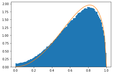
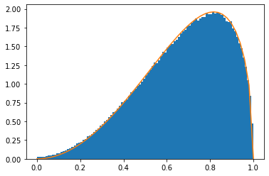
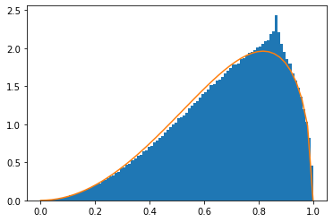
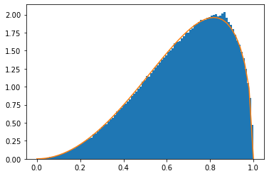
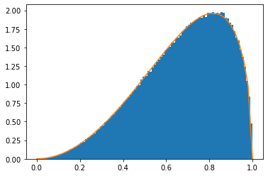
As the system decays to equilibrium and the distribution of the velocities approaches uniform, the marginal distributions become closer do dν3𝑑subscript𝜈3d\nu_{3}. In particular, by symmetry, we will only look at the radial component of this measure, which is proportional to r2(1r2)12drsuperscript𝑟2superscript1superscript𝑟212𝑑𝑟r^{2}(1-r^{2})^{\frac{1}{2}}dr. Additionally, the factorization formula and its symmetries reduce the conditional sampling problem to sampling from S2subscript𝑆2S_{2}, which is trivial. We refer to the radial distribution of the first particle as the sampled distribution, and the others as the implied distributions.

Thus, we can proceed as follows. Fixing the first coordinate, we sample r=|v|𝑟𝑣r=|v| from a given distribution using an acceptance/rejection mechanism, and sample y1subscript𝑦1y_{1}, y2subscript𝑦2y_{2} uniformly, so that the point is in S3subscript𝑆3S_{3}. We then let the system evolve sampling first the jump time and the particle that stays fixed, identified with 2v2𝑣\sqrt{2}v, and sample y1subscript𝑦1y_{1}, y2subscript𝑦2y_{2} uniformly on S2subscript𝑆2S_{2}.

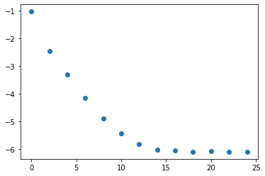
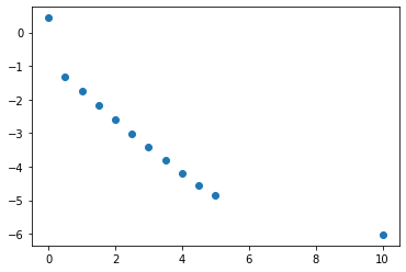
We perform 1 million simulations of the process in Python, for α=0,2𝛼02\alpha=0,2, and use these simulations to build a histogram approximating the probability distribution over 100 bins and several timestamps. We then measure the relative entropy between the empirical measure and the equilibrium radial measure over time, and use a log-plot to showcase and estimate the exponential decay. This was done over a selection of initial distributions, and a ”worst case scenario” is showcased here with the sampling distribution being 2(1x)21𝑥2(1-x), as most of the probability mass is concentrated close to zero.

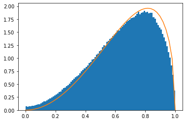
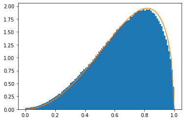
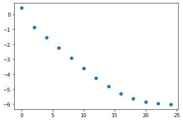
In figures 1, 2 and 3, the rather quick relaxation is evident. By computing the relative entropy using a first order Euler method, we see that there is a log-linear relationship up to a certain point, where the distributions are close enough so that the numerical approximations and random noise prevent the entropy from decaying below e6superscript𝑒6e^{-6}. Meanwhile, figures 4, 5 and 6 show the evolution of the distributions over several timestamps.
Refer to caption
Figure 1: α=2𝛼2\alpha=2, sampled entropy
Refer to caption
Figure 2: α=2𝛼2\alpha=2, implied entropy
Refer to caption
Figure 3: α=0𝛼0\alpha=0, sampled entropy
[Uncaptioned image]

t=0s

[Uncaptioned image]

t=0.5s

[Uncaptioned image]

t=2s

Refer to caption

t=3.5s

Refer to caption

t=5s

Refer to caption

t=10s

Figure 4: α=0𝛼0\alpha=0, sampled velocity
[Uncaptioned image]

t=0s

[Uncaptioned image]

t=2s

[Uncaptioned image]

t=6s

Refer to caption

t=10s

Refer to caption

t=16s

Refer to caption

t=24s

Figure 5: α=2𝛼2\alpha=2, sampled velocity
[Uncaptioned image]

t=0s

[Uncaptioned image]

t=2s

[Uncaptioned image]

t=6s

Refer to caption

t=10s

Refer to caption

t=16s

Refer to caption

t=24s

Figure 6: α=2𝛼2\alpha=2, implied velocity

3 Proof of the main result

3.1 The correlation operator on the sphere

The main result is based on careful analysis of the eigenfunctions and the spectrum of K𝐾K. We turn our attention to the study of this operator.

Let B𝐵B be the unit ball in 3superscript3{{\mathbb{R}}}^{3}, N3𝑁3N\geq 3, νNsubscript𝜈𝑁\nu_{N} as defined in (10) and consider the projections πk(v):SNB:subscript𝜋𝑘𝑣subscript𝑆𝑁𝐵\pi_{k}(\vec{v}):S_{N}\to B,

πk(v):=1N1vk.assignsubscript𝜋𝑘𝑣1𝑁1subscript𝑣𝑘\pi_{k}(\vec{v}):=\frac{1}{\sqrt{N-1}}v_{k}. (43)

By formula (7), we then have that

Bψ(v)𝑑νN=SNψ(πk(v))𝑑σN,subscript𝐵𝜓𝑣differential-dsubscript𝜈𝑁subscriptsubscript𝑆𝑁𝜓subscript𝜋𝑘𝑣differential-dsubscript𝜎𝑁\int_{B}\psi(v)d\nu_{N}=\int_{S_{N}}\psi(\pi_{k}(\vec{v}))d\sigma_{N},

for any integrable function ψ𝜓\psi on B𝐵B. We then define the operator K𝐾K on L2(B,νN)superscript𝐿2𝐵subscript𝜈𝑁L^{2}(B,\nu_{N}) by

ψ1,Kψ2L2(B,νN):=SNψ1(π1(v))ψ2(π2(v))𝑑σN.assignsubscriptsubscript𝜓1𝐾subscript𝜓2superscript𝐿2𝐵subscript𝜈𝑁subscriptsubscript𝑆𝑁superscriptsubscript𝜓1subscript𝜋1𝑣subscript𝜓2subscript𝜋2𝑣differential-dsubscript𝜎𝑁\langle\psi_{1},K\psi_{2}\rangle_{L^{2}(B,\nu_{N})}:=\int_{S_{N}}\psi_{1}^{*}(\pi_{1}(\vec{v}))\psi_{2}(\pi_{2}(\vec{v}))d\sigma_{N}. (44)

Note that the symmetries of the variables make K𝐾K self-adjoint. Furthermore, a simple rescaling, to extend K𝐾K to L2(σN)superscript𝐿2subscript𝜎𝑁L^{2}(\sigma_{N}), allows us to interpret this operator simply as a conditional expectation on the uniform sphere

Kξ(v)=𝔼[ξ(v1)|v2=v],𝐾𝜉𝑣𝔼delimited-[]conditional𝜉subscript𝑣1subscript𝑣2𝑣K\xi(v)={{\mathbb{E}}}[\xi(v_{1})|v_{2}=v],

but we will not consider this scaling as the former simplifies the treatment of eigenvalues.

Carlen, Carvalho and Loss make use of this operator to prove quantitative chaos estimates; that is, to quantify how far from independent the coordinates are, asymptotically in N𝑁N, and most of their work is based on extensive study of the spectrum of K𝐾K, built up over [3], [4].

Before we continue, define the functions

η0=1,ηj(v)=vj, for 1j3, and η4(v)=(|v|21)/(N1).formulae-sequenceformulae-sequencesubscript𝜂01formulae-sequencesubscript𝜂𝑗𝑣subscript𝑣𝑗 for 1𝑗3 and subscript𝜂4𝑣superscript𝑣21𝑁1\eta_{0}=1,\eta_{j}(v)=v_{j},\text{ for }1\leq j\leq 3,\text{ and }\eta_{4}(v)=(|v|^{2}-1)/(N-1). (45)

We will now present the most important facts obtained in these papers for general N𝑁N, and later turn to the our N=3𝑁3N=3 case. Following the results in [3], we have this next lemma:

Lemma 3.1

Let N3𝑁3N\geq 3. The operator K𝐾K is compact. The function η0subscript𝜂0\eta_{0} is an eigenfunction of K𝐾K with eigenvalue 1, and spans the corresponding eigenspace. The functions ηjsubscript𝜂𝑗\eta_{j}, for 1j41𝑗41\leq j\leq 4, are eigenfunctions with eigenvalue 1N11𝑁1-\frac{1}{N-1}, and they form an orthogonal basis for this subspace. No other eigenvalues of K𝐾K are larger in absolute value then 5N33(N1)35𝑁33superscript𝑁13\frac{5N-3}{3(N-1)^{3}}. Thus, for all ψL2(B,νN)𝜓superscript𝐿2𝐵subscript𝜈𝑁\psi\in L^{2}(B,\nu_{N}) orthogonal to these ηjsubscript𝜂𝑗\eta_{j},

Kψ225N33(N1)3ψ22.superscriptsubscriptnorm𝐾𝜓225𝑁33superscript𝑁13subscriptsuperscriptnorm𝜓22\|K\psi\|_{2}^{2}\leq\frac{5N-3}{3(N-1)^{3}}\|\psi\|^{2}_{2}. (46)

Finally, every eigenvalue κ𝜅\kappa of K𝐾K, other than 1, 1N11𝑁1-\frac{1}{N-1} and 5N33(N1)35𝑁33superscript𝑁13\frac{5N-3}{3(N-1)^{3}}, satisfies

7N33(N1)4κ5N33(N1)3.7𝑁33superscript𝑁14𝜅5𝑁33superscript𝑁13-\frac{7N-3}{3(N-1)^{4}}\leq\kappa\leq\frac{5N-3}{3(N-1)^{3}}. (47)

Unfortunately, these bounds are not enough when N=3𝑁3N=3 and are just slightly off to allow us to obtain the main result more easily. On the other hand, the authors also manage to establish that K𝐾K has a complete basis of eigenfunctions of the form

gn,,m=hn,(|v|)|v|𝒴,m(v/|v|),subscript𝑔𝑛𝑚subscript𝑛𝑣superscript𝑣subscript𝒴𝑚𝑣𝑣g_{n,\ell,m}=h_{n,\ell}(|v|)|v|^{\ell}\mathcal{Y}_{\ell,m}(v/|v|), (48)

where 𝒴,msubscript𝒴𝑚\mathcal{Y}_{\ell,m} denotes the \ell-th degree spherical harmonic and, with t=|v|21𝑡superscript𝑣21t=|v|^{2}-1, α=3N82(=12)𝛼annotated3𝑁82absent12\alpha=\frac{3N-8}{2}\bigg{(}=\frac{1}{2}\bigg{)} and β=+12𝛽12\beta=\ell+\frac{1}{2},

hn,(|v|)=Pn(α,β)(t),subscript𝑛𝑣superscriptsubscript𝑃𝑛𝛼𝛽𝑡h_{n,\ell}(|v|)=P_{n}^{(\alpha,\beta)}(t),

the n𝑛n-th degree Jacobi polynomial (recall that the Jacobi polynomials are the orthogonal polynomials on the interval [1,1]11[-1,1] for the weight (1x)α(1+x)βsuperscript1𝑥𝛼superscript1𝑥𝛽(1-x)^{\alpha}(1+x)^{\beta}). For convenience, we let capital P𝑃P denote these polynomials under Rodrigues’ normalization,

Pn(α,β)(t)=(1)n2nn(1x)α(1+x)βdndxn((1x)α+n(1+x)β+n),superscriptsubscript𝑃𝑛𝛼𝛽𝑡superscript1𝑛superscript2𝑛𝑛superscript1𝑥𝛼superscript1𝑥𝛽superscript𝑑𝑛𝑑superscript𝑥𝑛superscript1𝑥𝛼𝑛superscript1𝑥𝛽𝑛P_{n}^{(\alpha,\beta)}(t)=\frac{(-1)^{n}}{2^{n}n}(1-x)^{-\alpha}(1+x)^{-\beta}\frac{d^{n}}{dx^{n}}\bigg{(}(1-x)^{\alpha+n}(1+x)^{\beta+n}\bigg{)}, (49)

while pn(α,β)superscriptsubscript𝑝𝑛𝛼𝛽p_{n}^{(\alpha,\beta)} will correspond to the L2superscript𝐿2L^{2} orthonormal basis. Equation (48) also allows us to conclude that the spectrum of K𝐾K consists of eigenvalues κn,subscript𝜅𝑛\kappa_{n,\ell}, independent of m𝑚m and given by the explicit formula

κn,=Pn(α,β)(1+2(N1)2)Pn(α,β)(1)(1N1).subscript𝜅𝑛superscriptsubscript𝑃𝑛𝛼𝛽12superscript𝑁12superscriptsubscript𝑃𝑛𝛼𝛽1superscript1𝑁1\kappa_{n,\ell}=\frac{P_{n}^{(\alpha,\beta)}\Big{(}-1+\frac{2}{(N-1)^{2}}\Big{)}}{P_{n}^{(\alpha,\beta)}(1)}\bigg{(}-\frac{1}{N-1}\bigg{)}^{\ell}. (50)

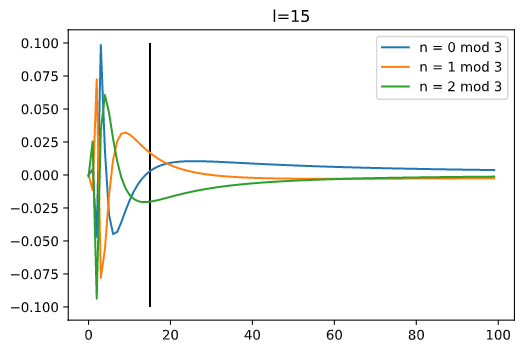
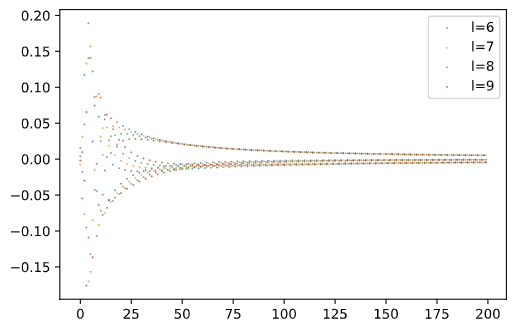
While similar formulas derived from the above were useful in the asymptotic N𝑁N case, a large amount of cancellation happens and makes the eigenvalues take values much smaller than implied by naive bounds. Furthermore, it appears that the eigenvalues display an explicit mod3moduloabsent3\mod 3 behavior. By this, we mean that for each \ell, plotting the eigenvalues for nmod3modulo𝑛3n\mod 3 separately yields 3 eventually monotonous sequences, as we can observe bellow:
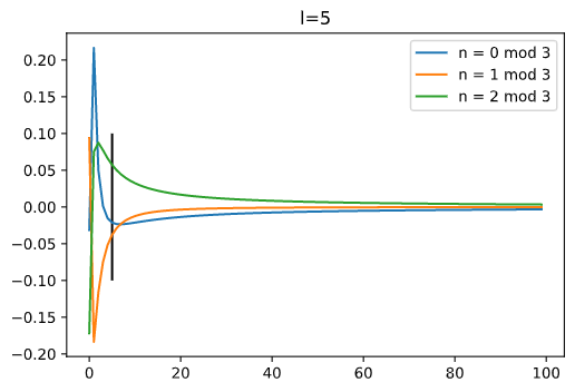
Refer to caption
Figure 7: First 300 values of κn,5subscript𝜅𝑛5\kappa_{n,5}
Refer to caption
Figure 8: First 300 values of κn,15subscript𝜅𝑛15\kappa_{n,15}
Refer to caption
Figure 9: Overlap of the plots from =66\ell=6 to 101010

As these 3 different behaviours are included simultaneously in the sequences, it further makes difficult the tasks of obtaining good uniform bounds.

One can also make use of the recurrence relations for Jacobi polynomials [10] to obtain the same type of relations for the eigenvalues κn,subscript𝜅𝑛\kappa_{n,\ell}. More precisely, for each \ell, we have that

12κn,=n++122n++1κn,1+n+122n++1κn+1,1.12subscript𝜅𝑛𝑛122𝑛1subscript𝜅𝑛1𝑛122𝑛1subscript𝜅𝑛11-\frac{1}{2}\kappa_{n,\ell}=\frac{n+\ell+\frac{1}{2}}{2n+\ell+1}\kappa_{n,\ell-1}+\frac{n+\frac{1}{2}}{2n+\ell+1}\kappa_{n+1,\ell-1}\ . (51)

Since we also know that

κn,0=1n+1(1)nsin(nπ3),subscript𝜅𝑛01𝑛1superscript1𝑛𝑛𝜋3\kappa_{n,0}=\frac{1}{n+1}(-1)^{n}\sin\bigg{(}\frac{n\pi}{3}\bigg{)}, (52)

this provides a fast and efficient way to at least numerically compute all the needed eigenvalues. We can, however, solve this recurrence relation in terms of the =00\ell=0 values, even if the obtained representation isn’t very useful:

κn,=(2)j=0(j)Cn,(j)κn+j,0,subscript𝜅𝑛superscript2superscriptsubscript𝑗0binomial𝑗superscriptsubscript𝐶𝑛𝑗subscript𝜅𝑛𝑗0\kappa_{n,\ell}=(-2)^{\ell}\sum_{j=0}^{\ell}\binom{\ell}{j}C_{n,\ell}^{(j)}\kappa_{n+j,0}\ , (53)

with

Cn,(j)=i=1{n+i+1/2}i=0,ij{2n+i+j+2}.superscriptsubscript𝐶𝑛𝑗superscriptsubscriptproduct𝑖1𝑛𝑖12superscriptsubscriptproductformulae-sequence𝑖0𝑖𝑗2𝑛𝑖𝑗2C_{n,\ell}^{(j)}=\frac{\prod_{i=1}^{\ell}\{n+i+1/2\}}{\prod_{i=0,i\neq j}^{\ell}\{2n+i+j+2\}}\ . (54)

One can see that the missing term in the denominator, when i=j𝑖𝑗i=j, is exactly 2 times the numerator of κn+j,0subscript𝜅𝑛𝑗0\kappa_{n+j,0}. Unfortunately, this representation shows no indication of decay, meaning that there is a large amount of cancellation occurring (the terms are large, but very close in absolute value). Collecting the sine terms may, however, shed some light on the mod3moduloabsent3\mod 3 question.

Thus, while explicit values of Jacobi polynomials are not trivial to compute, the authors make use of uniform pointwise bounds obtained by Nevai, Erdelyi and Magnus [9], a surprisingly deep result, to obtain monotonous bounds on these eigenvalues:

Lemma 3.2

We have that

κn,22eπg1(n,,N)g2(N)g3(n,N)g4(n,,N),subscriptsuperscript𝜅2𝑛2𝑒𝜋subscript𝑔1𝑛𝑁subscript𝑔2𝑁subscript𝑔3𝑛𝑁subscript𝑔4𝑛𝑁\kappa^{2}_{n,\ell}\leq\frac{2e}{\pi}g_{1}(n,\ell,N)g_{2}(N)g_{3}(n,N)g_{4}(n,\ell,N)\ , (55)

with

g1(n,,N)subscript𝑔1𝑛𝑁\displaystyle g_{1}(n,\ell,N) =(4+9N248N+65+42+43N+4n+25),absent49superscript𝑁248𝑁654superscript243𝑁4𝑛25\displaystyle=\bigg{(}\frac{4+\sqrt{9N^{2}-48N+65+4\ell^{2}+4\ell}}{3N+4n+2\ell-5}\bigg{)}\ ,
g2(N)subscript𝑔2𝑁\displaystyle g_{2}(N) =((N1)2N(N2))(3N7)/2,absentsuperscriptsuperscript𝑁12𝑁𝑁23𝑁72\displaystyle=\bigg{(}\frac{(N-1)^{2}}{N(N-2)}\bigg{)}^{(3N-7)/2}\ ,
g3(n,N)subscript𝑔3𝑛𝑁\displaystyle g_{3}(n,N) =Γ(n+1)Γ(32N3)Γ(n++32N52),absentΓ𝑛1Γ32𝑁3Γ𝑛32𝑁52\displaystyle=\frac{\Gamma(n+1)\Gamma(\frac{3}{2}N-3)}{\Gamma(n+\ell+\frac{3}{2}N-\frac{5}{2})}\ ,
g4(n,,N)subscript𝑔4𝑛𝑁\displaystyle g_{4}(n,\ell,N) =(N1)2Γ(n++32)Γ(32N3)Γ(n++32N52).absentsuperscript𝑁12Γ𝑛32Γ32𝑁3Γ𝑛32𝑁52\displaystyle=\frac{(N-1)^{2}\Gamma(n+\ell+\frac{3}{2})\Gamma(\frac{3}{2}N-3)}{\Gamma(n+\ell+\frac{3}{2}N-\frac{5}{2})}\ . (56)

This bound can be enlarged to allow for the monotonous behaviour. This time, however, when N=3𝑁3N=3, we are actually in a better position to further simplify the achieved bound, yielding

κn,28e3Γ(n+1)Γ(n+3/2)Γ(n++3/2)Γ(n++2)8e31(n+1)1/21(n++3/2)1/2=:κ^n,2.\kappa_{n,\ell}^{2}\leq\frac{8e}{3}\frac{\Gamma(n+1)}{\Gamma(n+3/2)}\frac{\Gamma(n+\ell+3/2)}{\Gamma(n+\ell+2)}\leq\frac{8e}{3}\frac{1}{(n+1)^{1/2}}\frac{1}{(n+\ell+3/2)^{1/2}}=:\hat{\kappa}_{n,\ell}^{2}\ . (57)

Now notice that, for all 44\ell\geq 4,

(n+1)(n++3/2)(n+)2,𝑛1𝑛32superscript𝑛2(n+1)(n+\ell+3/2)\geq(n+\sqrt{\ell})^{2}\ , (58)

so that if we define

κ~n,=8e31n+,subscript~𝜅𝑛8𝑒31𝑛\widetilde{\kappa}_{n,\ell}=\sqrt{\frac{8e}{3}}\frac{1}{\sqrt{n+\sqrt{\ell}}}\ , (59)

we have κ^n,κ~n,subscript^𝜅𝑛subscript~𝜅𝑛\hat{\kappa}_{n,\ell}\leq\widetilde{\kappa}_{n,\ell}. Both upper bounds will be useful later on. Inequality (57) is more precise, especially when we are looking for bounds independent of \ell. Nevertheless, inequality (59) has a far simpler representation and will be considered when we need to take derivatives.

3.2 Anti-symmetric sector

Now that we have built the necessary tools, we first treat the simpler anti-symmetric case, which can be done mostly through clever manipulation and simple bounds. We reproduce here the approach done in [2], with some minor numerical improvements.

Lemma 3.3

For N=3𝑁3N=3, the largest eigenvalue of P(2)superscript𝑃2P^{(2)} on the orthogonal complement of the symmetric sector is no larger than 0.7290.7290.729. Thus, either we have Δ^3,20.021subscript^Δ320.021\hat{\Delta}_{3,2}\geq 0.021 or else the gap eigenfunction is symmetric.

Suppose f𝑓f is anti-symmetric and we assume, without loss of generality, that f(v)=φ(v1)φ(v2)𝑓𝑣𝜑subscript𝑣1𝜑subscript𝑣2f(v)=\varphi(v_{1})-\varphi(v_{2}), with φ𝜑\varphi orthogonal to the constants. Then, P(2)f=λfsuperscript𝑃2𝑓𝜆𝑓P^{(2)}f=\lambda f becomes

1NwN,2(v1)(1K)φ(v1)1NwN,2(v2)(1K)φ(v2)=λ(φ(v1)φ(v2))1𝑁subscript𝑤𝑁2subscript𝑣11𝐾𝜑subscript𝑣11𝑁subscript𝑤𝑁2subscript𝑣21𝐾𝜑subscript𝑣2𝜆𝜑subscript𝑣1𝜑subscript𝑣2\frac{1}{N}w_{N,2}(v_{1})(1-K)\varphi(v_{1})-\frac{1}{N}w_{N,2}(v_{2})(1-K)\varphi(v_{2})=\lambda(\varphi(v_{1})-\varphi(v_{2})) (60)

Multiplying by φ(v1)𝜑subscript𝑣1\varphi(v_{1}) and integrating over 𝒮Nsubscript𝒮𝑁\mathcal{S}_{N}, we obtain

1N𝒮NwN,2(v1)|(1K)φ(v1)|2𝑑σN=λφ,(1K)φ.1𝑁subscriptsubscript𝒮𝑁subscript𝑤𝑁2subscript𝑣1superscript1𝐾𝜑subscript𝑣12differential-dsubscript𝜎𝑁𝜆𝜑1𝐾𝜑\frac{1}{N}\int_{\mathcal{S}_{N}}w_{N,2}(v_{1})|(1-K)\varphi(v_{1})|^{2}d\sigma_{N}=\lambda\langle\varphi,(1-K)\varphi\rangle. (61)

From

wN,2(vk)=NN1N(N1)2|vk|2,subscript𝑤𝑁2subscript𝑣𝑘𝑁𝑁1𝑁superscript𝑁12superscriptsubscript𝑣𝑘2w_{N,2}(v_{k})=\frac{N}{N-1}-\frac{N}{(N-1)^{2}}|v_{k}|^{2}, (62)

we can write (61) as

1N1φ,(1K)2φ1(N1)2(1K)φ,|v|2(1K)φ=λφ,(1K)φ1𝑁1𝜑superscript1𝐾2𝜑1superscript𝑁121𝐾𝜑superscript𝑣21𝐾𝜑𝜆𝜑1𝐾𝜑\frac{1}{N-1}\langle\varphi,(1-K)^{2}\varphi\rangle-\frac{1}{(N-1)^{2}}\langle(1-K)\varphi,|v|^{2}(1-K)\varphi\rangle=\lambda\langle\varphi,(1-K)\varphi\rangle (63)

After decomposing 1Kφ=ψ+ζ1𝐾𝜑𝜓𝜁\sqrt{1-K}\varphi=\psi+\zeta, where ψ𝜓\psi is orthogonal to the constants, the components vjsubscript𝑣𝑗v_{j} and |v|2superscript𝑣2|v|^{2}, we have that:

φ,(1K)2φ𝜑superscript1𝐾2𝜑\displaystyle\langle\varphi,(1-K)^{2}\varphi\rangle =ψ+ζ,(1K)(ψ+ζ)absent𝜓𝜁1𝐾𝜓𝜁\displaystyle=\langle\psi+\zeta,(1-K)(\psi+\zeta)\rangle
=ψ,(1K)ψ+(1+1/(N1))ζ22absent𝜓1𝐾𝜓11𝑁1subscriptsuperscriptnorm𝜁22\displaystyle=\langle\psi,(1-K)\psi\rangle+(1+1/(N-1))\|\zeta\|^{2}_{2}
=1Kψ22+NN1ζ22absentsubscriptsuperscriptnorm1𝐾𝜓22𝑁𝑁1subscriptsuperscriptnorm𝜁22\displaystyle=\|\sqrt{1-K}\psi\|^{2}_{2}+\frac{N}{N-1}\|\zeta\|^{2}_{2} (64)

and

(1K)φ,|v|2(1K)φ=1𝐾𝜑superscript𝑣21𝐾𝜑absent\displaystyle\langle(1-K)\varphi,|v|^{2}(1-K)\varphi\rangle= 1K(ψ+ζ),|v|21K(ψ+ζ)1𝐾𝜓𝜁superscript𝑣21𝐾𝜓𝜁\displaystyle\langle\sqrt{1-K}(\psi+\zeta),|v|^{2}\sqrt{1-K}(\psi+\zeta)\rangle
=\displaystyle= 1Kψ,|v|21Kψ+1Kζ,|v|21Kζ1𝐾𝜓superscript𝑣21𝐾𝜓1𝐾𝜁superscript𝑣21𝐾𝜁\displaystyle\langle\sqrt{1-K}\psi,|v|^{2}\sqrt{1-K}\psi\rangle+\langle\sqrt{1-K}\zeta,|v|^{2}\sqrt{1-K}\zeta\rangle
+\displaystyle+ 2|v|1Kψ,|v|1Kζ,2𝑣1𝐾𝜓𝑣1𝐾𝜁\displaystyle 2\langle|v|\sqrt{1-K}\psi,|v|\sqrt{1-K}\zeta\rangle, (65)

since ζ𝜁\zeta is an eigenfunction of K𝐾K with eigenvalue 1/(N1)1𝑁1-1/(N-1), it is also an eigenfunction of 1K1𝐾\sqrt{1-K}, with eigenvalue 1+1N1=NN111𝑁1𝑁𝑁1\sqrt{1+\frac{1}{N-1}}=\sqrt{\frac{N}{N-1}}.

It then follows that

1Kφ,|v|21Kφ1𝐾𝜑superscript𝑣21𝐾𝜑\displaystyle\langle\sqrt{1-K}\varphi,|v|^{2}\sqrt{1-K}\varphi\rangle 1Kψ,|v|21Kψ+1Kζ,|v|21Kζabsent1𝐾𝜓superscript𝑣21𝐾𝜓1𝐾𝜁superscript𝑣21𝐾𝜁\displaystyle\geq\langle\sqrt{1-K}\psi,|v|^{2}\sqrt{1-K}\psi\rangle+\langle\sqrt{1-K}\zeta,|v|^{2}\sqrt{1-K}\zeta\rangle
2|v|1Kψ|2NN1|v|ζ2evaluated-at2norm𝑣1𝐾𝜓2𝑁𝑁1subscriptnorm𝑣𝜁2\displaystyle-2\||v|\sqrt{1-K}\psi\||_{2}\sqrt{\frac{N}{N-1}}\||v|\zeta\|_{2}
(11t)1Kψ,|v|21Kψ+(1t)NN1|v|ζ22,absent11𝑡1𝐾𝜓superscript𝑣21𝐾𝜓1𝑡𝑁𝑁1superscriptsubscriptnorm𝑣𝜁22\displaystyle\geq\bigg{(}1-\frac{1}{t}\bigg{)}\langle\sqrt{1-K}\psi,|v|^{2}\sqrt{1-K}\psi\rangle+(1-t)\frac{N}{N-1}\||v|\zeta\|_{2}^{2}, (66)

using the Cauchy-Schwarz and arithmetic-geometric mean inequalities.

Before we move on, it is useful to note that |v|ζ22ζ22superscriptsubscriptnorm𝑣𝜁22subscriptsuperscriptnorm𝜁22\||v|\zeta\|_{2}^{2}\geq\|\zeta\|^{2}_{2}. To see this for N=3𝑁3N=3, write

ζ=j=14ajηj,𝜁superscriptsubscript𝑗14subscript𝑎𝑗subscript𝜂𝑗\zeta=\sum_{j=1}^{4}a_{j}\eta_{j}, (67)

with ηj(v)=𝒆jvsubscript𝜂𝑗𝑣subscript𝒆𝑗𝑣\eta_{j}(v)=\boldsymbol{e}_{j}\cdot v for j=1,2,3𝑗123j=1,2,3 and η4=|v|21subscript𝜂4superscript𝑣21\eta_{4}=|v|^{2}-1 as discussed in section 3.1.

From (67), a simple computation yields

|v|ζ22=j=14|aj|2|v|ηj22,subscriptsuperscriptnorm𝑣𝜁22superscriptsubscript𝑗14superscriptsubscript𝑎𝑗2subscriptsuperscriptnorm𝑣subscript𝜂𝑗22\||v|\zeta\|^{2}_{2}=\sum_{j=1}^{4}|a_{j}|^{2}\||v|\eta_{j}\|^{2}_{2}\ , (68)

and while a bit more cumbersome, one can also show that

𝒮3|v1|4𝑑σ3=54subscriptsubscript𝒮3superscriptsubscript𝑣14differential-dsubscript𝜎354\int_{\mathcal{S}_{3}}|v_{1}|^{4}d\sigma_{3}=\frac{5}{4} (69)

and

𝒮3|v1|6𝑑σ3=74.subscriptsubscript𝒮3superscriptsubscript𝑣16differential-dsubscript𝜎374\int_{\mathcal{S}_{3}}|v_{1}|^{6}d\sigma_{3}=\frac{7}{4}. (70)

Together, the equations above give us

|v|ηj22=54 for j=1,2,3 and |v|η4=1,formulae-sequencesubscriptsuperscriptnorm𝑣subscript𝜂𝑗2254 for 𝑗123 and norm𝑣subscript𝜂41\||v|\eta_{j}\|^{2}_{2}=\frac{5}{4}\text{ for }j=1,2,3\text{ and }\||v|\eta_{4}\|=1, (71)

which prove what we needed.

Finally, from the trivial bound 1Kψ,|v|21Kψ(N1)1Kψ221𝐾𝜓superscript𝑣21𝐾𝜓𝑁1subscriptsuperscriptnorm1𝐾𝜓22\langle\sqrt{1-K}\psi,|v|^{2}\sqrt{1-K}\psi\rangle\leq(N-1)\|\sqrt{1-K}\psi\|^{2}_{2}, we have that, for all 0<t<10𝑡10<t<1,

1Kφ,|v|21Kφ(11t)(N1)1Kψ22+(1t)NN1ζ22.1𝐾𝜑superscript𝑣21𝐾𝜑11𝑡𝑁1subscriptsuperscriptnorm1𝐾𝜓221𝑡𝑁𝑁1superscriptsubscriptnorm𝜁22\langle\sqrt{1-K}\varphi,|v|^{2}\sqrt{1-K}\varphi\rangle\geq\bigg{(}1-\frac{1}{t}\bigg{)}(N-1)\|\sqrt{1-K}\psi\|^{2}_{2}+(1-t)\frac{N}{N-1}\|\zeta\|_{2}^{2}\ . (72)

Specializing to N=3𝑁3N=3, the second most negative eigenvalue of K𝐾K is 3838-\frac{3}{8}, which yields 1Kψ22118ψ22subscriptsuperscriptnorm1𝐾𝜓22118subscriptsuperscriptnorm𝜓22\|\sqrt{1-K}\psi\|^{2}_{2}\leq\frac{11}{8}\|\psi\|^{2}_{2}. Combining all of the above,

λ(ψ22+ζ22)𝜆subscriptsuperscriptnorm𝜓22subscriptsuperscriptnorm𝜁22\displaystyle\lambda(\|\psi\|^{2}_{2}+\|\zeta\|^{2}_{2}) 12118ψ22+34ζ2212118(11t)ψ221432(1t)ζ22absent12118subscriptsuperscriptnorm𝜓2234subscriptsuperscriptnorm𝜁221211811𝑡subscriptsuperscriptnorm𝜓2214321𝑡subscriptsuperscriptnorm𝜁22\displaystyle\leq\frac{1}{2}\cdot\frac{11}{8}\|\psi\|^{2}_{2}+\frac{3}{4}\|\zeta\|^{2}_{2}-\frac{1}{2}\cdot\frac{11}{8}\bigg{(}1-\frac{1}{t}\bigg{)}\|\psi\|^{2}_{2}-\frac{1}{4}\frac{3}{2}(1-t)\|\zeta\|^{2}_{2}
=1116tψ22+38(1+t)ζ22.absent1116𝑡superscriptsubscriptnorm𝜓22381𝑡subscriptsuperscriptnorm𝜁22\displaystyle=\frac{11}{16t}\|\psi\|_{2}^{2}+\frac{3}{8}\bigg{(}1+t\bigg{)}\|\zeta\|^{2}_{2}\ . (73)

With t=0.943𝑡0.943t=0.943, this yields λ0.729𝜆0.729\lambda\leq 0.729.

3.3 Symmetric sector

The remaining task is to bound the second largest eigenvalue of P(2)superscript𝑃2P^{(2)} in the symmetric sector. Assume f𝑓f is of the form

f(v)=j=1Nφ(vj).𝑓𝑣superscriptsubscript𝑗1𝑁𝜑subscript𝑣𝑗f(\vec{v})=\sum_{j=1}^{N}\varphi(v_{j}). (74)

Then, we can write P(2)f=λfsuperscript𝑃2𝑓𝜆𝑓P^{(2)}f=\lambda f as

1Nj=1NwN,2(vj)(φ(vj)+(N1)Kφ(vj))=λj=1Nφ(vj).1𝑁superscriptsubscript𝑗1𝑁subscript𝑤𝑁2subscript𝑣𝑗𝜑subscript𝑣𝑗𝑁1𝐾𝜑subscript𝑣𝑗𝜆superscriptsubscript𝑗1𝑁𝜑subscript𝑣𝑗\frac{1}{N}\sum_{j=1}^{N}w_{N,2}(v_{j})(\varphi(v_{j})+(N-1)K\varphi(v_{j}))=\lambda\sum_{j=1}^{N}\varphi(v_{j}). (75)

Theorem 2.5 in [2] is here extremely important, as it allows us to treat the above sum component wise:

1NwN,2(v)(φ(v)+(N1)Kφ(v))=λφ(v).1𝑁subscript𝑤𝑁2𝑣𝜑𝑣𝑁1𝐾𝜑𝑣𝜆𝜑𝑣\frac{1}{N}w_{N,2}(v)(\varphi(v)+(N-1)K\varphi(v))=\lambda\varphi(v). (76)

By integrating against φ(v)𝜑𝑣\varphi(v), it follows that

1N𝒮Nφ(v1)wN,2(v1)(φ(v1)+(N1)Kφ(v1))𝑑σN=λφ22.1𝑁subscriptsubscript𝒮𝑁𝜑subscript𝑣1subscript𝑤𝑁2subscript𝑣1𝜑subscript𝑣1𝑁1𝐾𝜑subscript𝑣1differential-dsubscript𝜎𝑁𝜆subscriptsuperscriptnorm𝜑22\frac{1}{N}\int_{\mathcal{S}_{N}}\varphi(v_{1})w_{N,2}(v_{1})(\varphi(v_{1})+(N-1)K\varphi(v_{1}))d\sigma_{N}=\lambda\|\varphi\|^{2}_{2}. (77)

As, once again,

wN,2(v)=NN1N(N1)2|v|2,subscript𝑤𝑁2𝑣𝑁𝑁1𝑁superscript𝑁12superscript𝑣2w_{N,2}(v)=\frac{N}{N-1}-\frac{N}{(N-1)^{2}}|v|^{2}, (78)

and focusing on N=3𝑁3N=3, (77) becomes

λφ22𝜆subscriptsuperscriptnorm𝜑22\displaystyle\lambda\|\varphi\|^{2}_{2} =\displaystyle= 12𝒮3φ(v1)(112|v|2)(1+2K)φ(v1)𝑑σN12subscriptsubscript𝒮3𝜑subscript𝑣1112superscript𝑣212𝐾𝜑subscript𝑣1differential-dsubscript𝜎𝑁\displaystyle\frac{1}{2}\int_{\mathcal{S}_{3}}\varphi(v_{1})(1-\tfrac{1}{2}|v|^{2})(1+2K)\varphi(v_{1})d\sigma_{N} (79)
=\displaystyle= 12(112|v|2)φ,(1+2K)φ.12112superscript𝑣2𝜑12𝐾𝜑\displaystyle\frac{1}{2}\langle(1-\tfrac{1}{2}|v|^{2})\varphi,(1+2K)\varphi\rangle.

Since

1(112|v|2)1, (112|v|2)φ2φ2,formulae-sequence1112superscript𝑣21 subscriptnorm112superscript𝑣2𝜑2subscriptnorm𝜑2-1\leq\bigg{(}1-\frac{1}{2}|v|^{2}\bigg{)}\leq 1,\text{ }\bigg{\|}\bigg{(}1-\frac{1}{2}|v|^{2}\bigg{)}\varphi\bigg{\|}_{2}\leq\|\varphi\|_{2}, (80)

we obtain the first bound

λ121+2K2.𝜆12subscriptnorm12𝐾2\lambda\leq\frac{1}{2}\|1+2K\|_{2}. (81)

Unfortunately, this bound is useless as is, since the largest eigenvalue of K𝐾K, other than 111, is 1212\frac{1}{2}, giving us λ1𝜆1\lambda\leq 1. Thus, we need to be more incisive on the spectrum of K𝐾K and its interaction with the multiplication operator (112|v|2)112superscript𝑣2(1-\frac{1}{2}|v|^{2}).

Consider the operator

M:=|v|2(1+(N1)K).assign𝑀superscript𝑣21𝑁1𝐾M:=|v|^{2}(1+(N-1)K). (82)

Recalling the eigenbasis of K𝐾K,

gn,l,m=hn,l(|v|2)|v|l𝒴l,m(v/|v|),subscript𝑔𝑛𝑙𝑚subscript𝑛𝑙superscript𝑣2superscript𝑣𝑙subscript𝒴𝑙𝑚𝑣𝑣g_{n,l,m}=h_{n,l}(|v|^{2})|v|^{l}\mathcal{Y}_{l,m}(v/|v|), (83)

we see that M𝑀M commutes with rotations and thus different angular momentum sectors will be mutually orthogonal, so we can consider separately the dependence in \ell and m𝑚m (in fact, we will ignore m𝑚m completely, as gn,,msubscript𝑔𝑛𝑚g_{n,\ell,m}, gn,,msubscript𝑔𝑛superscript𝑚g_{n,\ell,m^{\prime}} belong to the same \ell-eigenspace). Thus, the quantities we are interested in estimating are

λ:=supφ=114(1t)φ,(1+2K)φ,assignsubscript𝜆subscriptsupremumnorm𝜑1141𝑡𝜑12𝐾𝜑\lambda_{\ell}:=\sup_{\|\varphi\|=1}\frac{1}{4}\langle(1-t)\varphi,(1+2K)\varphi\rangle, (84)

with the supremum being taken over the \ell sector. Moreover, as hn,l(|v|2)=Pn(α,β)(t)subscript𝑛𝑙superscript𝑣2superscriptsubscript𝑃𝑛𝛼𝛽𝑡h_{n,l}(|v|^{2})=P_{n}^{(\alpha,\beta)}(t), with t=|v|21𝑡superscript𝑣21t=|v|^{2}-1, β=l+12𝛽𝑙12\beta=l+\frac{1}{2}, we see that 112|v|2=12(1t)112superscript𝑣2121𝑡1-\frac{1}{2}|v|^{2}=\frac{1}{2}(1-t) in the Jacobi variables, and we can exploit the properties of Jacobi polynomials.

The slow simultaneous decay in n𝑛n and \ell we obtain from expressions like (59) pose an obstacle for computing meaningful bounds. Thus, we break down the problem over several ranges.

First, we look for a uniform bound given large enough >superscript\ell>\ell^{*}, but such that superscript\ell^{*} is as small as possible.

For 5<<5superscript5<\ell<\ell^{*}, the eigenvalues are already small enough for (81) to work as well, and we make use of a uniform bound in n𝑛n to reduce this problem to explicitly computing a finite amount of these. Note that the recurrence formula (recurrence) makes this fairly trivial and efficient.

Finally, we provide an argument based on linear algebra for 55\ell\leq 5, where closed form expressions are simple enough for this.

3.3.1 Large \ell case

Let fn,,msubscript𝑓𝑛𝑚f_{n,\ell,m} be a re-scaling of gn,,msubscript𝑔𝑛𝑚g_{n,\ell,m} such that the basis is orthonormal, and fix \ell, m𝑚m.

Writing Pn:=Pn(α,β)assignsubscript𝑃𝑛superscriptsubscript𝑃𝑛𝛼𝛽P_{n}:=P_{n}^{(\alpha,\beta)}, the three-term relation for Jacobi polynomials [10] is

Pn+1(t)=(Ant+Bn)Pn(t)+CnPn1(t),subscript𝑃𝑛1𝑡subscript𝐴𝑛𝑡subscript𝐵𝑛subscript𝑃𝑛𝑡subscript𝐶𝑛subscript𝑃𝑛1𝑡P_{n+1}(t)=(A_{n}t+B_{n})P_{n}(t)+C_{n}P_{n-1}(t)\ , (85)

with

Ansubscript𝐴𝑛\displaystyle A_{n} =(2n+α+β+1)(2n+α+β+2)2(n+1)(n+α+β+1),absent2𝑛𝛼𝛽12𝑛𝛼𝛽22𝑛1𝑛𝛼𝛽1\displaystyle=\frac{(2n+\alpha+\beta+1)(2n+\alpha+\beta+2)}{2(n+1)(n+\alpha+\beta+1)}\ ,
Bnsubscript𝐵𝑛\displaystyle B_{n} =(α2β2)(2n+α+β+1)2(n+1)(n+α+β+1)(2n+α+β),absentsuperscript𝛼2superscript𝛽22𝑛𝛼𝛽12𝑛1𝑛𝛼𝛽12𝑛𝛼𝛽\displaystyle=\frac{(\alpha^{2}-\beta^{2})(2n+\alpha+\beta+1)}{2(n+1)(n+\alpha+\beta+1)(2n+\alpha+\beta)}\ ,
Cnsubscript𝐶𝑛\displaystyle C_{n} =(n+α)(2n+α+β+2)(n+β)(n+1)(n+α+β+1)(2n+α+β),absent𝑛𝛼2𝑛𝛼𝛽2𝑛𝛽𝑛1𝑛𝛼𝛽12𝑛𝛼𝛽\displaystyle=\frac{(n+\alpha)(2n+\alpha+\beta+2)(n+\beta)}{(n+1)(n+\alpha+\beta+1)(2n+\alpha+\beta)}\ , (86)

which gives

tPn=(1/An)Pn+1(Bn/An)Pn+(Cn/An)Pn1.𝑡subscript𝑃𝑛1subscript𝐴𝑛subscript𝑃𝑛1subscript𝐵𝑛subscript𝐴𝑛subscript𝑃𝑛subscript𝐶𝑛subscript𝐴𝑛subscript𝑃𝑛1tP_{n}=(1/A_{n})P_{n+1}-(B_{n}/A_{n})P_{n}+(C_{n}/A_{n})P_{n-1}\ . (87)

As we are working with orthonormal functions, we have to re-scale the equality. By the orthogonality relations for Jacobi polynomials,

Pn(α,β),Pn(α,β)L2(μ(α,β))=2α+β+12n+α+β+1Γ(n+α+1)Γ(n+β+1)Γ(n+α+β+1)n!δnm,subscriptsuperscriptsubscript𝑃𝑛𝛼𝛽superscriptsubscript𝑃𝑛𝛼𝛽superscript𝐿2superscript𝜇𝛼𝛽superscript2𝛼𝛽12𝑛𝛼𝛽1Γ𝑛𝛼1Γ𝑛𝛽1Γ𝑛𝛼𝛽1𝑛subscript𝛿𝑛𝑚\langle P_{n}^{(\alpha,\beta)},P_{n}^{(\alpha,\beta)}\rangle_{L^{2}(\mu^{(\alpha,\beta)})}=\frac{2^{\alpha+\beta+1}}{2n+\alpha+\beta+1}\frac{\Gamma(n+\alpha+1)\Gamma(n+\beta+1)}{\Gamma(n+\alpha+\beta+1)n!}\delta_{nm}\ , (88)

we first compute

Pn(α,β)22=2α+β+12n+α+β+1Γ(n+α+1)Γ(n+β+1)Γ(n+α+β+1)n!,superscriptsubscriptnormsuperscriptsubscript𝑃𝑛𝛼𝛽22superscript2𝛼𝛽12𝑛𝛼𝛽1Γ𝑛𝛼1Γ𝑛𝛽1Γ𝑛𝛼𝛽1𝑛\displaystyle\|P_{n}^{(\alpha,\beta)}\|_{2}^{2}=\frac{2^{\alpha+\beta+1}}{2n+\alpha+\beta+1}\frac{\Gamma(n+\alpha+1)\Gamma(n+\beta+1)}{\Gamma(n+\alpha+\beta+1)n!}\ ,
Pn1(α,β)22Pn(α,β)22=2n++22n+n(n++1)(n+1/2)(n++1/2),superscriptsubscriptnormsuperscriptsubscript𝑃𝑛1𝛼𝛽22superscriptsubscriptnormsuperscriptsubscript𝑃𝑛𝛼𝛽222𝑛22𝑛𝑛𝑛1𝑛12𝑛12\displaystyle\frac{\|P_{n-1}^{(\alpha,\beta)}\|_{2}^{2}}{\|P_{n}^{(\alpha,\beta)}\|_{2}^{2}}=\frac{2n+\ell+2}{2n+\ell}\frac{n(n+\ell+1)}{(n+1/2)(n+\ell+1/2)}\ ,
Pn+1(α,β)22Pn(α,β)22=2n++22n++4(n+3/2)(n++3/2)(n+1)(n++2).superscriptsubscriptnormsuperscriptsubscript𝑃𝑛1𝛼𝛽22superscriptsubscriptnormsuperscriptsubscript𝑃𝑛𝛼𝛽222𝑛22𝑛4𝑛32𝑛32𝑛1𝑛2\displaystyle\frac{\|P_{n+1}^{(\alpha,\beta)}\|_{2}^{2}}{\|P_{n}^{(\alpha,\beta)}\|_{2}^{2}}=\frac{2n+\ell+2}{2n+\ell+4}\frac{(n+3/2)(n+\ell+3/2)}{(n+1)(n+\ell+2)}\ . (89)

Defining the scaling factors

Fnsuperscriptsubscript𝐹𝑛\displaystyle F_{n}^{-} :=Pn1Pn=n(2n+α+β+1)(n+α+β)(n+α)(n+β)(2n+α+β1),assignabsentnormsubscript𝑃𝑛1normsubscript𝑃𝑛𝑛2𝑛𝛼𝛽1𝑛𝛼𝛽𝑛𝛼𝑛𝛽2𝑛𝛼𝛽1\displaystyle:=\frac{\|P_{n-1}\|}{\|P_{n}\|}=\sqrt{\frac{n(2n+\alpha+\beta+1)(n+\alpha+\beta)}{(n+\alpha)(n+\beta)(2n+\alpha+\beta-1)}}\ ,
Fn+subscriptsuperscript𝐹𝑛\displaystyle F^{+}_{n} :=Pn+1Pn=(n+α+1)(n+β+1)(2n+α+β+1)(n+1)(n+α+β+1)(2n+α+β+3),assignabsentnormsubscript𝑃𝑛1normsubscript𝑃𝑛𝑛𝛼1𝑛𝛽12𝑛𝛼𝛽1𝑛1𝑛𝛼𝛽12𝑛𝛼𝛽3\displaystyle:=\frac{\|P_{n+1}\|}{\|P_{n}\|}=\sqrt{\frac{(n+\alpha+1)(n+\beta+1)(2n+\alpha+\beta+1)}{(n+1)(n+\alpha+\beta+1)(2n+\alpha+\beta+3)}}\ , (90)

the three-term relation for the multiplication operator in the orthonormal Jacobi polynomials is

tpn=cnpn1+anpn+bnpn+1,𝑡subscript𝑝𝑛subscript𝑐𝑛subscript𝑝𝑛1subscript𝑎𝑛subscript𝑝𝑛subscript𝑏𝑛subscript𝑝𝑛1tp_{n}=c_{n}p_{n-1}+a_{n}p_{n}+b_{n}p_{n+1}, (91)

with

an:=BnAnbn:=Fn+Ancn:=FnCnAn.assignsubscript𝑎𝑛subscript𝐵𝑛subscript𝐴𝑛subscript𝑏𝑛assignsubscriptsuperscript𝐹𝑛subscript𝐴𝑛subscript𝑐𝑛assignsubscriptsuperscript𝐹𝑛subscript𝐶𝑛subscript𝐴𝑛a_{n}:=-\frac{B_{n}}{A_{n}}\text{, }b_{n}:=\frac{F^{+}_{n}}{A_{n}}\text{, }c_{n}:=\frac{F^{-}_{n}C_{n}}{A_{n}}. (92)

Notice that, by the self-adjointness of multiplication by t𝑡t, we must have cn=bn1subscript𝑐𝑛subscript𝑏𝑛1c_{n}=b_{n-1}. After some algebraic manipulation, we verify this and also obtain

bn,=2(n+1)(n+3/2)(n++3/2)(n++2)(2n++2)(2n++3)2(2n++4),subscript𝑏𝑛2𝑛1𝑛32𝑛32𝑛22𝑛2superscript2𝑛322𝑛4b_{n,\ell}=2\sqrt{\frac{(n+1)(n+3/2)(n+\ell+3/2)(n+\ell+2)}{(2n+\ell+2)(2n+\ell+3)^{2}(2n+\ell+4)}}, (93)
an,=(+1)(2n++1)(2n++3).subscript𝑎𝑛12𝑛12𝑛3a_{n,\ell}=\frac{\ell(\ell+1)}{(2n+\ell+1)(2n+\ell+3)}. (94)

Evidently an,a~n,subscript𝑎𝑛subscript~𝑎𝑛a_{n,\ell}\geq\widetilde{a}_{n,\ell} where

a~n,:=(2n++3)2=(12n+32n++3)2.assignsubscript~𝑎𝑛superscript2𝑛32superscript12𝑛32𝑛32\widetilde{a}_{n,\ell}:=\left(\frac{\ell}{2n+\ell+3}\right)^{2}=\left(1-\frac{2n+3}{2n+\ell+3}\right)^{2}\ . (95)

It is clear that a~n,subscript~𝑎𝑛\widetilde{a}_{n,\ell} is decreasing in n𝑛n and increasing in \ell. It will also be useful to have a bound on bn,subscript𝑏𝑛b_{n,\ell} that is simpler to estimate. For this, notice that we can pair the ’close’ terms in the numerator, and compare with those in the denominator. We then have

bn,subscript𝑏𝑛absent\displaystyle b_{n,\ell}\leq 2(n+3/2)2(n++2)2(2n++2)2(2n++3)2=2n+32n++3n++22n++22superscript𝑛322superscript𝑛22superscript2𝑛22superscript2𝑛322𝑛32𝑛3𝑛22𝑛2\displaystyle 2\sqrt{\frac{(n+3/2)^{2}(n+\ell+2)^{2}}{(2n+\ell+2)^{2}(2n+\ell+3)^{2}}}=\frac{2n+3}{2n+\ell+3}\frac{n+\ell+2}{2n+\ell+2}
=\displaystyle= (12n++3)(1n2n++2)(12n++3)(1n2n++3).12𝑛31𝑛2𝑛212𝑛31𝑛2𝑛3\displaystyle\bigg{(}1-\frac{\ell}{2n+\ell+3}\bigg{)}\bigg{(}1-\frac{n}{2n+\ell+2}\bigg{)}\leq\bigg{(}1-\frac{\ell}{2n+\ell+3}\bigg{)}\bigg{(}1-\frac{n}{2n+\ell+3}\bigg{)}\ . (96)

We therefore define

b~n,:=(12n++3)(1n2n++3).assignsubscript~𝑏𝑛12𝑛31𝑛2𝑛3\widetilde{b}_{n,\ell}:=\bigg{(}1-\frac{\ell}{2n+\ell+3}\bigg{)}\bigg{(}1-\frac{n}{2n+\ell+3}\bigg{)}\ . (97)

In order to better understand the behaviour of these sequences, we treat them as functions of continuous variables. Differentiating in \ell we find

b~n,=(2+6)n+3+9(2n++3)3,subscript~𝑏𝑛26𝑛39superscript2𝑛33\frac{{\partial}}{{\partial}\ell}\widetilde{b}_{n,\ell}=-\frac{(2\ell+6)n+3\ell+9}{(2n+\ell+3)^{3}}\ , (98)

so that b~n,subscript~𝑏𝑛\widetilde{b}_{n,\ell} is decreasing in \ell. Differentiating in n𝑛n, we see that

nb~n,=22+3(6n+9)(2n++3)3,𝑛subscript~𝑏𝑛2superscript236𝑛9superscript2𝑛33\frac{{\partial}}{{\partial}n}\widetilde{b}_{n,\ell}=\frac{2\ell^{2}+3\ell-(6n+9)}{(2n+\ell+3)^{3}}\ , (99)

so that b~n,subscript~𝑏𝑛\widetilde{b}_{n,\ell} is increasing in n𝑛n for

n22+396.𝑛2superscript2396n\leq\frac{2\ell^{2}+3\ell-9}{6}\ .

Suppose now φ𝜑\varphi belongs to the (,m)𝑚(\ell,m) angular momentum sector, so that we can expand it as

φ=n=0+φnfn,,m.𝜑superscriptsubscript𝑛0subscript𝜑𝑛subscript𝑓𝑛𝑚\varphi=\sum_{n=0}^{+\infty}\varphi_{n}f_{n,\ell,m}\ . (100)

Observing that

(1+2K)φ=n=1+(1+2kn,)φnfn,,m,12𝐾𝜑superscriptsubscript𝑛112subscript𝑘𝑛subscript𝜑𝑛subscript𝑓𝑛𝑚\displaystyle(1+2K)\varphi=\sum_{n=1}^{+\infty}(1+2k_{n,\ell})\varphi_{n}f_{n,\ell,m}\ , (101)
(1t)φ=n=1+(bn1φn1+(1an)φn+cn+1φn+1)fn,,m,1𝑡𝜑superscriptsubscript𝑛1subscript𝑏𝑛1subscript𝜑𝑛11subscript𝑎𝑛subscript𝜑𝑛subscript𝑐𝑛1subscript𝜑𝑛1subscript𝑓𝑛𝑚\displaystyle(1-t)\varphi=\sum_{n=1}^{+\infty}(b_{n-1}\varphi_{n-1}+(1-a_{n})\varphi_{n}+c_{n+1}\varphi_{n+1})f_{n,\ell,m}\ , (102)

we finally derive

(1t)φ,(1+2K)φ=1𝑡𝜑12𝐾𝜑absent\displaystyle\langle(1-t)\varphi,(1+2K)\varphi\rangle= n=1+bn1,(1+2kn,)φn1φnsuperscriptsubscript𝑛1subscript𝑏𝑛112subscript𝑘𝑛subscript𝜑𝑛1subscript𝜑𝑛\displaystyle-\sum_{n=1}^{+\infty}b_{n-1,\ell}(1+2k_{n,\ell})\varphi_{n-1}\varphi_{n}
+n=1+(1an,)(1+2kn,)φn2superscriptsubscript𝑛11subscript𝑎𝑛12subscript𝑘𝑛superscriptsubscript𝜑𝑛2\displaystyle+\sum_{n=1}^{+\infty}(1-a_{n,\ell})(1+2k_{n,\ell})\varphi_{n}^{2}
n=1+bn,(1+2kn,)φn+1φn.superscriptsubscript𝑛1subscript𝑏𝑛12subscript𝑘𝑛subscript𝜑𝑛1subscript𝜑𝑛\displaystyle-\sum_{n=1}^{+\infty}b_{n,\ell}(1+2k_{n,\ell})\varphi_{n+1}\varphi_{n}\ . (103)

Taking the supremum on each term and using Cauchy-Schwarz on the φnφn±1subscript𝜑𝑛subscript𝜑plus-or-minus𝑛1\varphi_{n}\varphi_{n\pm 1} terms yields, and recalling the upper bound (59) κn,κ~n,subscript𝜅𝑛subscript~𝜅𝑛\kappa_{n,\ell}\leq\widetilde{\kappa}_{n,\ell},

λsubscript𝜆\displaystyle\lambda_{\ell} 14[2supn{bn,(1+2κn,)}+supn{(1an,)(1+2κn,)}]absent14delimited-[]2subscriptsupremum𝑛subscript𝑏𝑛12subscript𝜅𝑛subscriptsupremum𝑛1subscript𝑎𝑛12subscript𝜅𝑛\displaystyle\leq\frac{1}{4}\bigg{[}2\sup_{n}\{b_{n,\ell}(1+2\kappa_{n,\ell})\}+\sup_{n}\{(1-a_{n,\ell})(1+2\kappa_{n,\ell})\}\bigg{]}
14[2supn{b~n,(1+2κ~n,)}+supn{(1a~n,)(1+2κ~n,)}].absent14delimited-[]2subscriptsupremum𝑛subscript~𝑏𝑛12subscript~𝜅𝑛subscriptsupremum𝑛1subscript~𝑎𝑛12subscript~𝜅𝑛\displaystyle\leq\frac{1}{4}\bigg{[}2\sup_{n}\{\widetilde{b}_{n,\ell}(1+2\widetilde{\kappa}_{n,\ell})\}+\sup_{n}\{(1-\widetilde{a}_{n,\ell})(1+2\widetilde{\kappa}_{n,\ell})\}\bigg{]}. (104)

We can then turn our attention to the sequences b~n,(1+2κ~n,)subscript~𝑏𝑛12subscript~𝜅𝑛\widetilde{b}_{n,\ell}(1+2\widetilde{\kappa}_{n,\ell}) and (1a~n,)(1+2κ~n,)1subscript~𝑎𝑛12subscript~𝜅𝑛(1-\widetilde{a}_{n,\ell})(1+2\widetilde{\kappa}_{n,\ell}).

Proposition 3.1

For all 7070\ell\geq 70, λ0.73016subscript𝜆0.73016\lambda_{\ell}\leq 0.73016.

Proof –   We first compute the derivative in n𝑛n of (1a~n,)(1+2κ~n,)1subscript~𝑎𝑛12subscript~𝜅𝑛(1-\widetilde{a}_{n,\ell})(1+2\widetilde{\kappa}_{n,\ell}), which we find

42346e+3n+(2n++3)3n+23(1k2(2n++3)2)6e(n+)3/2.4superscript2346𝑒3𝑛superscript2𝑛33𝑛231superscript𝑘2superscript2𝑛326𝑒superscript𝑛32\frac{4\ell^{2}}{3}\frac{4\sqrt{6e}+3\sqrt{n+\sqrt{\ell}}}{(2n+\ell+3)^{3}\sqrt{n+\sqrt{\ell}}}-\frac{2}{3}\frac{\left(1-\frac{k^{2}}{(2n+\ell+3)^{2}}\right)\sqrt{6e}}{(n+\sqrt{\ell})^{3/2}}\ .

which has the same sign as

2246e+3n+(2n++3)3(1k2(2n++3)2)6en+.2superscript246𝑒3𝑛superscript2𝑛331superscript𝑘2superscript2𝑛326𝑒𝑛{2\ell^{2}}\frac{4\sqrt{6e}+3\sqrt{n+\sqrt{\ell}}}{(2n+\ell+3)^{3}}-\frac{\left(1-\frac{k^{2}}{(2n+\ell+3)^{2}}\right)\sqrt{6e}}{n+\sqrt{\ell}}\ . (105)

Now assume n3/2𝑛superscript32n\geq\ell^{3/2}. Then, we have that 22(2n++3)4/32superscript2superscript2𝑛343{2\ell^{2}}\leq(2n+\ell+3)^{4/3}, n+(2n++3)1/2𝑛superscript2𝑛312\sqrt{n+\sqrt{\ell}}\leq(2n+\ell+3)^{1/2}, and

k2(2n++3)214.superscript𝑘2superscript2𝑛3214\frac{k^{2}}{(2n+\ell+3)^{2}}\leq\frac{1}{4\ell}\ .

Thus, when n3/2𝑛superscript32n\geq\ell^{3/2}, the quantity in (105) is bounded above by

46e/+3(n+)7/6(114)6en+.46𝑒3superscript𝑛761146𝑒𝑛\frac{4\sqrt{6e/\sqrt{\ell}}+3}{(n+\sqrt{\ell})^{7/6}}-\frac{\left(1-\frac{1}{4\ell}\right)\sqrt{6e}}{n+\sqrt{\ell}}\ .

Hence our derivative is negative when n3/2𝑛superscript32n\geq\ell^{3/2} and

(n+)1/646e/+3(114)6e.superscript𝑛1646𝑒31146𝑒(n+\sqrt{\ell})^{1/6}\geq\frac{4\sqrt{6e/\sqrt{\ell}}+3}{\left(1-\frac{1}{4\ell}\right)\sqrt{6e}}\ .

For =7070\ell=70, this is satisfied for n86𝑛86n\geq 86, and 703/2586superscript703258670^{3/2}\leq 586. Hence, for =7070\ell=70, (1a~n,)(1+2κ~n,)1subscript~𝑎𝑛12subscript~𝜅𝑛(1-\widetilde{a}_{n,\ell})(1+2\widetilde{\kappa}_{n,\ell}) is decreasing in n𝑛n for al n586𝑛586n\geq 586, and these values of n𝑛n and \ell is it less than 1.221.221.22. Checking the finitely many remaining cases, one finds that the maximum occurs at n=66𝑛66n=66, and is less than 1.43511.43511.4351.

Proceeding similarly for 2b~n,(1+2κ~n,)2subscript~𝑏𝑛12subscript~𝜅𝑛2\widetilde{b}_{n,\ell}(1+2\tilde{\kappa}_{n,\ell}) we find the for =7070\ell=70, the maximum occurs at n=53𝑛53n=53, and is no more than 1.48551.48551.4855. Altogether we find,

λ701.4855+1.435140.73016.subscript𝜆701.48551.435140.73016\lambda_{70}\leq\frac{1.4855+1.4351}{4}\leq 0.73016\ .

Since it is clear that bn,(1+2κ~,)b_{n,\ell}(1+2\tilde{\kappa}_{,\ell}) and (1an,)(1+2κ~n,)1subscript𝑎𝑛12subscript~𝜅𝑛(1-a_{n,\ell})(1+2\tilde{\kappa}_{n,\ell}) are decreasing in \ell, this proves that λ0.73016subscript𝜆0.73016\lambda_{\ell}\leq 0.73016 for all 7070\ell\geq 70.

3.3.2 Small \ell

By inequality (59), and ignoring the dependence in \ell, we see that for n151𝑛151n\geq 151 we have κn,0.23subscript𝜅𝑛0.23\kappa_{n,\ell}\leq 0.23. Numerically checking, this holds as well for all 6506506\leq\ell\leq 50 and 0n1510𝑛1510\leq n\leq 151. Thus, for 5<<705705<\ell<70, the norm of Ksubscript𝐾K_{\ell}, the restriction of K𝐾K to the \ell angular momentum sector satisfies

K0.23.normsubscript𝐾0.23\|K_{\ell}\|\leq 0.23\ .

It follows from (81) that for 5<<705705<\ell<70,

λ12(1+20.23)=0.73.subscript𝜆12120.230.73\lambda_{\ell}\leq\frac{1}{2}(1+2\cdot 0.23)=0.73\ .

Taking into consideration the \ell dependency can also help reduce the amount of cases needed to check.

This leaves only the =0,1,2,3,4,5012345\ell=0,1,2,3,4,5 cases. Below, we provide a computation for =00\ell=0, making use of the explicit expressions obtained via (51) and (52). The same computation can be carried out analogously for the remaining cases, at the expense of explicitly computing the three term relation factors and the eigenvalues, and taking an appropriate choice of index for a break point.

For =00\ell=0, the operator φ(v)(112|v|2)φ(v)maps-to𝜑𝑣112superscript𝑣2𝜑𝑣\varphi(v)\mapsto(1-\tfrac{1}{2}|v|^{2})\varphi(v) is given in the Jacobi basis by the matrix

X:=14[2100012100012100012100012].assign𝑋14delimited-[]2100012100012100012100012X:=\frac{1}{4}\left[\begin{array}[]{cccccc}\phantom{-}2&-1&\phantom{-}0&\phantom{-}0&\phantom{-}0&\dots\\ -1&\phantom{-}2&-1&\phantom{-}0&\phantom{-}0&\dots\\ \phantom{-}0&-1&\phantom{-}2&-1&\phantom{-}0&\dots\\ \phantom{-}0&\phantom{-}0&-1&\phantom{-}2&-1&\dots\\ \phantom{-}0&\phantom{-}0&\phantom{-}0&-1&\phantom{-}2&\dots\\ \phantom{-}\vdots&\phantom{-}\vdots&\phantom{-}\vdots&\phantom{-}\vdots&\vdots&\ddots\end{array}\right]\ .

Let Y𝑌Y be the diagonal matrix whose n𝑛nth diagonal entry is 1+2κn+1,012subscript𝜅𝑛101+2\kappa_{n+1,0}. The upper 5×5555\times 5 block of Z:=12(YX+XY)assign𝑍12𝑌𝑋𝑋𝑌Z:=\frac{1}{2}(YX+XY) is

[1251600051634218000021803101500015122700027914].delimited-[]1251600051634218000021803101500015122700027914\left[\begin{array}[]{ccccc}\phantom{-}\frac{1}{2}&-\frac{5}{16}&\phantom{-}0&\phantom{-}0&\phantom{-}0\\ -\frac{5}{16}&\phantom{-}\frac{3}{4}&-\frac{21}{80}&\phantom{-}0&\phantom{-}0\\ \phantom{-}0&-\frac{21}{80}&\phantom{-}\frac{3}{10}&-\frac{1}{5}&\phantom{-}0\\ \phantom{-}0&\phantom{-}0&-\frac{1}{5}&\phantom{-}\frac{1}{2}&-\frac{2}{7}\\ \phantom{-}0&\phantom{-}0&\phantom{-}0&-\frac{2}{7}&\phantom{-}\frac{9}{14}\end{array}\right]\ .

According to Maple, the largest eigenvalue of this matrix is less than 1.04121.04121.0412. We also have that

Z6,5=Z5,6=57224.subscript𝑍65subscript𝑍5657224Z_{6,5}=Z_{5,6}=-\frac{57}{224}\ .

Let φ𝜑\varphi be any unit vector in 2superscript2\ell^{2}, and let η𝜂\eta be the vector with ηj=φjsubscript𝜂𝑗subscript𝜑𝑗\eta_{j}=\varphi_{j} for j=1,2,3,4𝑗1234j=1,2,3,4, and ηj=0subscript𝜂𝑗0\eta_{j}=0 for j>4𝑗4j>4. Let ζ:=φηassign𝜁𝜑𝜂\zeta:=\varphi-\eta. Then

φ,Zφ=η,Z^η+ζ,Zζ572242φ4φ5.𝜑𝑍𝜑𝜂^𝑍𝜂𝜁𝑍𝜁572242subscript𝜑4subscript𝜑5\langle\varphi,Z\varphi\rangle=\langle\eta,\widehat{Z}\eta\rangle+\langle\zeta,Z\zeta\rangle-\frac{57}{224}2\varphi_{4}\varphi_{5}\ .

We have

η,Z^η1.0412η2,𝜂^𝑍𝜂1.0412superscriptnorm𝜂2\langle\eta,\widehat{Z}\eta\rangle\leq 1.0412\|\eta\|^{2}\ ,

and by the Schwarz argument, since the largest relevant eigenvalue of K𝐾K is 110110\tfrac{1}{10},

ζ,Zζ65ζ2.𝜁𝑍𝜁65superscriptnorm𝜁2\langle\zeta,Z\zeta\rangle\leq\frac{6}{5}\|\zeta\|^{2}\ .

Thus, φ,Zφ𝜑𝑍𝜑\langle\varphi,Z\varphi\rangle is less than the largest eigenvalue of

[1.0412572245722465],delimited-[]1.0412572245722465\left[\begin{array}[]{cc}1.0412&-\frac{57}{224}\\ -\frac{57}{224}&\frac{6}{5}\end{array}\right]\ ,

which is no more than 1.3881.3881.388. Dividing by 222, we get our bound on the top eigenvalue in the =00\ell=0 sector, 0.6940.6940.694.

4 Conclusion

Comparing the bounds obtained in each sector, theorem 2.1 follows. Obviously, the result is only as good as the worst bound we obtain. While a bound of 0.020.020.02 is certainly achievable as we have seen, it is not clear if this method could yield a much better result.

Nevertheless, we appear to be off by one order of magnitude, which is decent enough, and we saw how the erratic behaviour of the eigenvalues κn,subscript𝜅𝑛\kappa_{n,\ell} poses an obstacle towards this.

Thus, a future goal would be proving entropy production inequalities with non-degenerate ’constants’, first for the conjugate process and possibly for the Kac process itself following Villani’s work. This is out of reach at the moment, and careful geometrical analysis is needed due to the state space constraints.

It is possible, however, that these quantities can be related analogously to their respective spectral gaps, and new insights can be obtained this way.

Appendix A Small \ell computations

For =1,,515\ell=1,...,5, we may proceed exactly the same way as for the =00\ell=0 case. Recall that, through the recurrence relation (51), we are able to obtain explicit formulas for eigenvalues in each \ell sector. For instance, we can always write κn,subscript𝜅𝑛\kappa_{n,\ell} as a linear combination of κn,0subscript𝜅𝑛0\kappa_{n,0}, κn+1,0subscript𝜅𝑛10\kappa_{n+1,0}, …, κn+,0subscript𝜅𝑛0\kappa_{n+\ell,0}, and we see that

κn,1subscript𝜅𝑛1\displaystyle\kappa_{n,1} =(κn,0+κn+1,0),absentsubscript𝜅𝑛0subscript𝜅𝑛10\displaystyle=-(\kappa_{n,0}+\kappa_{n+1,0})\ , (106)
κn,2subscript𝜅𝑛2\displaystyle\kappa_{n,2} =n+5/2n+2κn,0+κn+1,0+n+3/2n+2κn+2,0.absent𝑛52𝑛2subscript𝜅𝑛0subscript𝜅𝑛10𝑛32𝑛2subscript𝜅𝑛20\displaystyle=\frac{n+5/2}{n+2}\kappa_{n,0}+\kappa_{n+1,0}+\frac{n+3/2}{n+2}\kappa_{n+2,0}\ . (107)

Once again, these simplify if we consider separate cases given nmod3modulo𝑛3n\mod 3, and analogous formulas hold for =3,4,5345\ell=3,4,5, but with 4, 5 and 6 terms respectively.

We begin by computing the upper 5×5555\times 5 block of the Z𝑍Z matrix, as well as its largest eigenvalue, and note the remainder entries that separate it from the lower block (the coefficient of the φ5φ6subscript𝜑5subscript𝜑6\varphi_{5}\varphi_{6} term). Finally, we compute the largest relevant eigenvalue κn,subscript𝜅𝑛\kappa_{n,\ell} for the Schwarz argument.

This procedure is represented in the table below, with fractions denoting the exact values and decimals as close upper bounds.

\ell Upper block bound Remainder Largest κn,subscript𝜅𝑛\kappa_{n,\ell} Eigenvalue bound
0 1.0412 -57/224 1/10 0.694
1 0.946 -0.2729 1/8 0.7052
2 0.895 -0.2084 0.12 0.669
3 0.81 -0.254 0.105 0.667
4 0.784 -0.2275 0.12 0.6671
5 0.754 -0.206 0.1 0.6403

Appendix B Python code for the Monte Carlo simulations

We leave in this appendix the Python code that was used for the Monte Carlo simulations of the α=2𝛼2\alpha=2 case, as the only difference in the Maxwellian case are the constant jump rates 1/N1𝑁1/N. Please note that the code is not optimized and vast memory and run time improvements could be made. The helper functions are defined as close as possible to our theoretical conventions and notations.

N = 3
def norm_2(v):
return sum([x**2 for x in v])
def exp_sample(lamb=1):
u = np.random.rand()
X = -np.log(1-u)/lamb
return X
def lamb(v):
l = [0]*N
for i in range(N):
l[i] = (N**2 - (1 + norm_2(v[i]))*N)/( N*(N-1)**2 )
return l
def sample_jump_time(v):
params_ = lamb(v)
jump_time = exp_sample( params_[0] )
jump_index = 0
for i in range(1,N):
candidate = exp_sample( params_[i] )
if candidate < jump_time:
jump_time = candidate
jump_index = i
return jump_time, jump_index
def beta(v):
return np.sqrt(3/2 * (1-norm_2(v)))
def conditional_jump_to_uniform3(vel,index):
new_vel = vel
v = vel[index]/np.sqrt(2)
y1 = np.random.normal(size=3)
y2 = -y1
scale = (np.sqrt(norm_2(y1)+norm_2(y2)))/np.sqrt(2)
y1 = y1/scale
y2 = y2/scale
if index == 0:
new_vel[1] = beta(v)*y1 - v/np.sqrt(2)
new_vel[2] = beta(v)*y2 - v/np.sqrt(2)
elif index == 1:
new_vel[0] = beta(v)*y1 - v/np.sqrt(2)
new_vel[2] = beta(v)*y2 - v/np.sqrt(2)
elif index == 2:
new_vel[0] = beta(v)*y1 - v/np.sqrt(2)
new_vel[1] = beta(v)*y2 - v/np.sqrt(2)
return new_vel
n_sim = 1000000
sim_count = 0
frames = [2, 4, 6, 8, 10, 12, 14, 16, 18, 20, 22, 24]
first_sample = []
first_sample2 = []
first_sample3 = []
final_sample = [[] for x in range(12)]
final_sample2 = [[] for x in range(12)]
final_sample3 = [[] for x in range(12)]
index_dist = [[] for x in range(12)]
while sim_count < n_sim:
r = np.random.rand()
u = np.random.rand()
while u > (1-r):
r = np.random.rand()
u = np.random.rand()
v = np.random.normal(size=3)
v = r*v/np.sqrt(norm_2(v))
first_sample.append(2*r)
# initialize the remaining coordinates according to the parametrization
v2 = np.random.normal(size=3)
v3 = -v2
scale = (np.sqrt(norm_2(v2)+norm_2(v3)))/np.sqrt(2)
v2 = v2/scale
v3 = v3/scale
vel = [np.sqrt(2)*v,beta(v)*v2 - v/np.sqrt(2), beta(v)*v3 - v/np.sqrt(2)]
first_sample2.append(norm_2(vel[1]))
first_sample3.append(norm_2(vel[2]))
t = 0
for i in range(len(frames)):
T = frames[i]
while t<T:
tau, index = sample_jump_time(vel)
index_dist[i].append(index)
t += tau
vel = conditional_jump_to_uniform3(vel, index)
final_sample[i].append(np.sqrt(norm_2(vel[0])))
final_sample2[i].append(np.sqrt(norm_2(vel[1])))
final_sample3[i].append(np.sqrt(norm_2(vel[2])))
sim_count += 1
entropy = []
first_dist = [x/2 for x in first_sample]
counts, bins, bars = plt.hist(first_dist, bins=100, density=True)
ent = sum([counts[i]*np.log(counts[i]/(5.09295817894*(bins[i])**2 *
(1-bins[i]**2)**(1/2)))/100 for i in range(1,len(counts))])
entropy.append(ent)
x = np.linspace(0,1)
plt.plot(x, 5.09295817894*x**2 * (1-x**2)**(1/2))
plt.show()
for i in range(12):
final_dist = [x/np.sqrt(2) for x in final_sample[i]]
counts, bins, bars = plt.hist(final_dist, bins=100, density=True)
ent = [counts[i]/100 * np.log( counts[i] /
((bins[i])**2*(1-bins[i]**2)**(1/2)*5.09295817894))
for i in range(1,len(counts))]
total_ent = sum(ent)
entropy.append(total_ent)
plt.plot(x, 5.09295817894*x**2 * (1-x**2)**(1/2))
plt.show()
frames0 = [0, 2, 4, 6, 8, 10, 12, 14, 16, 18, 20, 22, 24]
plt.scatter(frames0, y = np.log(entropy))

References

  • [1] M. Kac., Foundations of kinetic theory, Proc. 3rd Berkley symp. Math. Stat. Prob., J. Neyman, ed. Univ. of California, vol 3, (1956) 171-197
  • [2] E. A. Carlen, M. C. Carvalho and M. Loss, Spectral gaps for reversible Markov processes with chaotic invariant measures: the Kac process with hard sphere collisions in three dimensions, arXiv:1812.03874 [math-ph]
  • [3] E. A. Carlen, J. S. Geronimo and M. Loss, Determination of the spectral gap in the Kac model for physical momentum and energy conserving collisions, arXiv:0705.3729 [math-ph]
  • [4] E. A. Carlen, J. S. Geronimo and M. Loss, On the Markov sequence problem for Jacobi polynomials, Advances in Mathematics, Volume 226, Issue 4, (2011) 3426-3466.
  • [5] E. Janvresse, Spectral Gap for Kac’s model of Boltzmann Equation, Annals. of Prob., Volume 29, (2001) 288-304.
  • [6] C. Villani, Cercignani’s Conjecture is Sometimes True and Always Almost True, Comm. Math. Phys., Volume 234, (2003) 455–490.
  • [7] F. Barthe, D. Cordero-Erausquin and B. Maurey, Entropy of spherical marginals and related inequalities, Jour. de Math., Pures et Appliquées, Volume 86, (2006) 89–99.
  • [8] E. A. Carlen, E. H. Lieb, and M. Loss, A sharp analog of Youngs inequality on SN and related entropy inequalities, J. Geom. Anal., Volume 14, (2004) 487–520.
  • [9] P. Nevai, T. Erdélyi and A. Magnus, Generalized Jacobi weights, Christoffel functions and Jacobi polynomials, SIAM Jour. Math. Anal., Volume 25, (1994) 602–614.
  • [10] G. Szegö, Orthogonal Polynomials, American Mathematical Society Colloquium Publications, ,Volume 23, AMS, Providence R.I. 193