Hierarchical Reinforcement Learning with Optimal Level Synchronization based on a Deep Generative Model

Abstract

The high-dimensional or sparse reward task of a reinforcement learning (RL) environment requires a superior potential controller such as hierarchical reinforcement learning (HRL) rather than an atomic RL because it absorbs the complexity of commands to achieve the purpose of the task in its hierarchical structure. One of the HRL issues is how to train each level policy with the optimal data collection from its experience. That is to say, how to synchronize adjacent level policies optimally. Our research finds that a HRL model through the off-policy correction technique of HRL, which trains a higher-level policy with the goal of reflecting a lower-level policy which is newly trained using the off-policy method, takes the critical role of synchronizing both level policies at all times while they are being trained. We propose a novel HRL model supporting the optimal level synchronization using the off-policy correction technique with a deep generative model. This uses the advantage of the inverse operation of a flow-based deep generative model (FDGM) to achieve the goal corresponding to the current state of the lower-level policy. The proposed model also considers the freedom of the goal dimension between HRL policies which makes it the generalized inverse model of the model-free RL in HRL with the optimal synchronization method. The comparative experiment results show the performance of our proposed model.

I Introduction

Of the many reinforcement learning (RL) algorithms, hierarchical reinforcement learning (HRL) compensates for the disadvantage of an atomic RL such as the Monte-Carlo policy gradient (REINFORCE) [1], deterministic policy gradient algorithm (DPG) [2], deep Q-network (DQN) [3], deep deterministic policy gradient algorithm (DDPG) [4], soft actor-critic (SAC) [5], and the twin delayed deep deterministic algorithm (TD3) [6] since it has a strong capability to seek an optimal solution efficiently in a high-dimensional state and action or a sparse reward environment. It achieves competitive performance in these areas thanks to a temporal abstraction goal which is a hierarchical optimal action between the policies of HRL. Since HRL is composed of hierarchical policies, the communication between a higher-level policy and a lower-level policy is critical for the performance of HRL. In the case of a two-level hierarchical structure, while the higher-level policy focuses on the abstract and generalized features, the lower-level policy works on the primitive action coupled with an environment (see Fig. 1 showing the Ant environment which is used in this research).

In a goal-conditioned HRL, a policy is conditioned on the other input called a goal which is sent from its higher-level policy. Due to the importance of the communication role between each HRL policy, there are several ways to handle a HRL algorithm from the viewpoint of controlling a goal. For instance, a HRL algorithm controls a goal by using an atomic RL algorithm [7, 8] or various machine learning algorithms [9, 10, 11]. The goal is also used for training its own policy.

One of the concerning HRL issues is how to train each policy with optimal data collection for the purpose of the task. The off-policy correction in HRL was suggested in [7] as an alternative solution regarding the optimal training issue in HRL. It is the combination of off-policy and correction in terms of how to train a higher-level policy from the viewpoint of the current lower-level policy. One of its components, i.e. correction, should be examined carefully. Off-policy has been under the spotlight because it can overcome the local minima of the on-policy. On the contrary, the off-policy has a non-stationary issue regarding training a higher-level policy of HRL because of its innate algorithm characteristic.

Previous research [7] has tried to solve this issue using various indirect methods which do not consider the state of the policy. The research in [7] proposes an off-policy correction to overcome the issue of off-policy by relabelling the past experience which is the action of the higher-level policy. However, this method has not proved to be proper or exact due to its limitations. The work in [7] makes use of a probabilistic method. It is not enough for the method to reflect the latest state of the lower-level policy exactly since it is only an indirect estimate. Our research focuses on the importance of a direct method using the exact reflection of the current state of a policy, which improves the effectiveness of training.

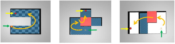
Figure 1: An example of several tasks in the Ant environment used in this research. The target location (yellow arrow) is the reward point for the approach of the agent, ant (green arrow). A trained policy requires the combination of various actions of the agent and its interplay with an object in the environment (pink blocks) in each task: the series of several directional movements (third from right), clearing away the obstacle (second from right) and making a bridge with an object (right). A higher-level policy guides its lower-level policy to be rewarded with an abstract action (orange arrow) which includes the desired positions and orientation of the ant and its limbs.

In our research, we propose a novel HRL model ensuring the level synchronization by the off-policy correction using the state of the policy to exactly reflect a lower-level policy without using superficial data such as an indirect method. To reflect the internal state of a lower-level policy in the off-policy correction, the state of a present neural network should be used in the computation. Using the inverse of a policy is the best way for the goal to be computed from the policy in a direct way for relabelling a previous goal of a higher-level policy. If the value of an inverse operation of a lower-level policy in terms of an action is evaluated as a goal of higher-level policy reflecting the state of the current lower-level policy, the method utilizing the inverse model of a policy can become an actual and accurate off-policy correction method of HRL. That is to say, finding the inverse value of a policy of a model-free RL in HRL is defined as an inverse model of a model-free RL in HRL.

A deep generative model is an appropriate way to find the inverse value of a policy. Except for the flow-based deep generative model (FDGM), other deep generative models are not good candidates for defining an inverse model in HRL since they incur a high cost because of their intrinsic mechanism. Yet, an FDGM supports the exact inverse value of a policy without the problem of other deep generative methods. However, an FDGM has an inherent restriction between the input and output dimension and also has a chronic defect, a biased log-density estimate. The former makes it difficult to define the inverse model which uses a general method to support the flexible choice of a goal dimension without a constraint. A large body of research is being conducted to overcome the latter in FDGM. Our research considers an architecture devised from one of the existing solutions to the latter to take advantage of the merits of FDGM in HRL in spite of its disadvantages.

Using an optimal off-policy correction in HRL to synchronize each level of HRL after it is trained, one should answer the following questions. How can the off-policy correction in HRL be operated using the internal state of a newly trained lower-level policy for the optimal training of its higher-level policy? How can one address the disadvantage of a FDGM when it is considered for a lower-level policy in order to use its inverse operation for relabelling a goal for off-policy correction? How can the freedom of the goal dimension be ensured for various commands of a higher-level policy in the off-policy correction when an FDGM is considered for our model? Is it possible to use the suggested model as a general inverse model of the model-free RL in HRL?

To summarize, our research introduces a novel HRL model architecture to define an inverse model of the model-free RL in HRL that uses an FDGM for off-policy correction. We take advantage of the inverse operation of an FDGM for the purpose of off-policy correction in HRL. In contrast to the previous method proposed in [7], our model pursues a direct method to find the exact goal reflecting the state of a newly updated lower-level policy for relabelling the previous goal of its higher-level policy. To evaluate our model, we use the same environment, which includes several tasks, as in the previous research [7]. Our results are compared with the results of HIRO [7] in terms of speed and accuracy. The results show the superior ability of our model over HIRO.

II Preliminary Knowledge

II-A Hierarchical reinforcement learning

The structure of HRL is composed of several unit agents which are stacked hierarchically. A policy of goal-conditioned HRL has two inputs which are the state of an environment $s_{t}$ and a goal $g_{t}$, which is a temporal abstraction, sent from its higher-level policy $\mu_{hi}$. A unit agent is usually constructed on an atomic RL since it acts as a policy in a level of HRL. The lowest-level policy communicates with an environment by its action $a_{t}\sim\mu_{lo}(s_{t},g_{t})$ based on the goal $g_{t}$ of its higher-level policy which is $g_{t}\sim\mu_{hi}$ every c time steps (c is the horizon of $\mu_{hi}$) or of a fixed goal transition function h($s_{t-1},g_{t-1},s_{t}$). The training period of a higher-level policy $\mu_{hi}$, c, is longer than that of its lower-level policy $\mu_{lo}$ due to the hierarchical structure. The higher a policy is located in a HRL, the more abstract the policy is. An environment reacts to the action of a lowest-level policy $a_{t}$ of a HRL with a reward $\textit{R}_{t}$ and a next state $s_{t+1}$ sampled from its reward function R($s_{t},a_{t}$) and its transition function f($s_{t},a_{t}$) respectively. The intrinsic reward $\textit{r}_{t}$ = r($s_{t},g_{t},a_{t}s_{t+1}$) for a lower-level policy in a HRL, except for the highest-level policy which uses a reward $\textit{R}_{t}$ of an environment, is usually supplied by a higher-level policy.

II-B Off-policy correction

It is significant that an optimal training solution is devised to enhance the performance of HRL. The off-policy in HRL has been proposed after its importance emerged due to the local minimum issue of an on-policy. In the off-policy policy gradient, the experience replay which is a sampled trajectory data of a past episode stored in a replay buffer results in improved sample efficiency. We can achieve better exploration results from a sample collection of a behaviour policy which is different from a target policy. The objective function of the off-policy policy gradient is as follows,

$$J(\theta)=\mathbb{E}_{S\sim d^{\beta}}\left[\sum_{a\in{A}}Q^{\pi}(s,a)\pi_{\theta}(a|s)\right]$$

where $\textit{d}^{\beta}(s)$ is the stationary distribution of the behaviour policy $\beta(a|s)$, $\pi_{\theta}(a|s)$ is the target policy and $\textit{Q}^{\pi}(s,a)$ is the action-value function estimated regarding the target policy $\pi_{\theta}(a|s)$ [12]. The innate characteristic of an off-policy causes a loss of synchronization of the training of hierarchical policies. Since a higher-level policy does not recognize how to reply the change of its lower-level policy in an off-policy after the lower-level policy is trained, a sampled goal, stored in a replay buffer of the higher-level policy, may not produce the same previous action of a lower-level policy when the higher-level policy is trained, which was the action of the lower policy according to the goal of the higher-level policy in the past. In other words, after a lower-level policy in HRL is trained and then changed, a higher-level policy, which is being trained in a bottom-up network-wise method usually accepted in HRL, should know whether a goal taken from the replay buffer is optimal for the newly changed policy or not since the newly changed lower-level policy may not have the same action of the previous lower-level policy by a previous goal sent from the higher-level policy.

To overcome the issue of the off-policy in HRL, the research in [7] proposed a method to relabel the experience of a higher-level policy which is stored in a replay buffer for the off-policy. The research shows how to relabel goal $g_{t}$ of the higher-level policy, which is stored in the replay buffer and used for training a higher-level policy, with an estimated goal $\tilde{g}_{t}$ reflecting the state of a newly updated lower-level policy when a higher-level policy is trained. The method makes use of a probabilistic method using the state given from an environment and the previous goal generated by a higher-level policy.

III Related work

III-A Hierarchical RL

A large body of researche has focused on developing an optimal method to connect adjacent level policies in the HRL framework from an action point of view. However, the existing research does not consider the optimal training for the level synchronization between adjacent level policies. Option-critic architecture learns internal policies autonomously, a condition of option termination and policies over options. The policy over options chooses an option to follow its intra policy which continues to work until the condition of option termination is reached [13]. The strategic attentive writer with the structure of HRL has an advantage over the sequential decision making domain due to the macro-action which is partially organized depending on environment information [14]. FeUdal networks (FuNs) for HRL have strength in a task of long-term credit assignment by having a decoupled module for a manager through a dilated LSTM and a worker with an intrinsic reward. In addition, FuNs acknowledges semantically meaningful sub-goals in an environment followed by different policies of the manager [15]. [9] suggests an efficient and general method to discover a sub-goal with two unsupervised learning methods, anomaly outlier detection and K-means clustering. The hierarchical Actor-Critic has DDPG with an actor-critic network and Hindsight Experience Replay [16] on every policy [17]. [18] introduces a nested and goal-conditioned HRL framework which can divide a task into several sub tasks with two classes of hindsight transition. The representation learning mapping from an observation space to a goal space in goal-conditioned HRL is important so as to reach an optimal policy. [19] developed a method to utilize representation learning through sub-optimality which is defined as the difference between the value function of an optimal HRL which does not utilize representation learning and the value function of an HRL which utilizes representation learning.

The main focus of the following research is to find an effective training method for each HRL policy regarding the dynamics of training between adjacent level policies to synchronize each other. The work in [7] defines a general goal, a parameterized reward function for a lower-level policy and an off-policy correction for HRL for a sample-efficiency. Our research extends the work begun in [7] on the off-policy correction which is the most interesting part of our research. In order to find $g_{t}\in{R^{d_{s}}}$ for an off-policy correction in HRL, HIRO finds 10 candidates which are eight candidate goals sampled randomly from a Gaussian centred at the distance of state $s_{t+c}-s_{t}$ between the horizon of the higher level policy ‘c’, an original goal $g_{t}$ and the distance of state $s_{t+c}-s_{t}$. Ten candidates are evaluated in an induced log probability of a lower level policy,

$$\log\mu_{lo}(a_{t:t+c-1}|s_{t:t+c-1},\tilde{g}_{t:t+c-1})$$

$$\propto -\frac{1}{2}\sum_{i=t}^{t+c-1}\|a_{i}-\mu_{lo}(s_{i},\tilde{g}_{i})\|_{2}^{2}+\text{const}.$$

In order to find the best candidate, in the end, the best goal is used for training the higher-level policy. The research considers three other methods detailed in the Appendix. Yet, it still does not propose a proper method for off-policy correction of the model-free RL in HRL. Therefore, our research is most interested in developing a model which supports the optimal selection of the goal in a direct way which reflects the state of a policy in mode-free RL in HRL. [8] suggests that each policy in HRL can be trained based on a bottom-up layer-wise way through a latent variable which is incorporated in the maximum entropy objective. Furthermore, for a higher level to retain full expressivity, the research takes advantage of an FDGM. For our purposes, our research embraces the use of an FDGM in HRL similar to [8].

III-B Deep generative models

GAN and VAE

[20] proposed an innovative deep generative model, Generative Adversarial Nets (GAN), which has two models, a discriminator and a generator. A Variational AutoEncoder (VAE) [21] has a probabilistic encoder which generates a latent variable for a decoder to overcome the shortcomings of the vanilla Autoencoder [22]. Lots of variants of these two generative models have been developed because of their outstanding unsupervised learning framework [23, 24, 25, 26, 27, 28, 29]. But GAN has the biggest defect leading to a training divergence because it cannot find a Nash equilibrium easily [30]. Although VAE supports precise control over the latent variable, it also has a blurry output due to a drawback of imperfect reconstruction which results in difficulty training the decoder. Because of the innate disadvantages of GAN and VAE, they are avoided in our research.

Normalizing Flow

A simple distribution can be transformed into a complex distribution by repeatedly using an invertible mapping function. The change of the variable theorem makes the transformation from a variable to a new one possible and leads to the final distribution of the target variable as follows. Suppose a probability density function $z\sim q(z)$ for a random variable $z$. If an invertible bijective transformation function $f$ exists between a new variable $x$ and $z$, $x=f(z)$ and $z=f^{-1}(x)$. Again, if the change of the variable theorem is applied to x and z in the multivariate version,

$$\textbf{z}_{i-1}\sim q_{i-1}(\textbf{z}_{i-1}),\leavevmode\nobreak\ \textbf{z}_{i}=f_{i}(\textbf{z}_{i-1}),\leavevmode\nobreak\ \textbf{z}_{i-1}=f_{i}^{-1}(\textbf{z}_{i})$$

and then

$$q_{i}(\textbf{z}_{i})= q_{i-1}(f_{i}^{-1}(\textbf{z}_{i}))\left|\frac{df_{i}^{-1}}{d\textbf{z}_{i}}\right|,$$

$$\log{q_{i}(\textbf{z}_{i})}= \log{q_{i-1}(\textbf{z}_{i-1})-\log{\left|\frac{df_{i}}{d\textbf{z}_{i-1}}\right|}}.$$

Finally, the chain of K transformations of probability density function $f_{\textmd{i}}$, which is easily inverted and whose Jacobian determinant can be easily computed, from the initial distribution $\textbf{z}_{0}$ yields a final target variable x,

x $$=\textbf{z}_{\textmd{K}}=f_{\textmd{K}}\circ\circ\circ f_{2}\circ f_{1}(\textbf{z}_{0})$$

$$\log{p(\textbf{x})} =\log{q_{\textmd{K}}(\textbf{z}_{\textmd{K}})}=\log{q_{0}(\textbf{z}_{0})-\sum_{i=1}^{\textmd{K}}\log{\left|\frac{df_{i}}{d\textbf{z}_{i-1}}\right|}}$$

In our research, we focus on the advantages of a normalizing flow, which are model flexibility and generation speed, even though it also has drawbacks. A Real-valued Non-Volume Preserving algorithm (RealNVP) makes use of a normalizing flow which is implemented with an invertible bijective transformation function. Each bijection called an affine coupling layer, which is $f:\textbf{x}\mapsto\textbf{y}$, decomposes an input dimension into two sections. The intrinsic transformation property using the affine coupling layer causes the input dimension to be unchanged with the alternate modification of the two split input sections in each coupling layer. Based on this property, the inverse operation is attained without difficulty. In addition, the inverse operation easily computes its Jacobian determinant since its Jacobian is a lower triangular matrix. RealNVP uses a multi-scale architecture as well as a batch normalization for better performance. To support a local correlation structure of an image, there are two masked convolution methods: the spatial checkerboard pattern mask and channel-wise mask [31]. Non-linear Independent Components Estimation (NICE) which is a previous model of RealNVP uses an additive coupling layer which does not use the scale term of an affine coupling layer [32]. Generative flow with 1$\times$1 convolutions (Glow) is a method to simplify the architecture regarding a reverse operation of channel ordering of NICE and RealNVP [33].

Several studies have tried to overcome the chronic drawback of a normalizing flow, biased log-density estimation [34, 35]. [36] utilizes the intrinsic characteristic of FDGM with an inductive bias based on a model architecture. Hence, the research takes advantage of a biased log-density estimation of FDGM itself. The research suggests a model architecture using a VAE which extracts a global representation of an image and a FDGM, which depends on a local representation, with a conditional input of the global representation of the image. Finally, an unbiased log-density estimation of an image can be expected from the FDGM using the output of the VAE. We adopt this architecture as the main idea for our model. The model architecture is as follows. The compression encoder

$$q_{\phi}(z|x)$$

in the VAE framework compresses the image x with a high dimension to the latent representation z with a low dimension. Then to reconstruct x using a flow-based decoder

$$v=f_{\theta}(x;z)$$

where a latent representation z, which is the output of the compression encoder, is fed into the flow-based decoder as a conditional input for dealing with the biased log-density estimation of FDGM. Finally, image x is reconstructed by using the inverse function

$$x=f_{\theta}^{-1}(v;z).$$

Auto-regressive flow

An auto-regressive flow provides tractable likelihoods due to the observable probability of a full sequence given by the product of conditional past probabilities so that it has a better density estimation than non-autoregressive flow-based models [37, 38, 39, 40, 41]. Yet, the restoration speed of the original data which results from its operation countervails its merit.

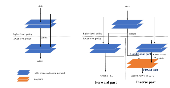
Figure 2: The architecture of our suggested model using FDGM (right) compared with HIRO (left)

IV Our model

Our research concentrates on the general HRL model supporting the level synchronization in multi-level HRL using off-policy correction based on FDGM. In other words, our model can be applied on any level of an HRL. Yet, for the simplicity of the experiment benchmark in our research, we utilize a two-level hierarchical structure.

The off-policy correction reflects the current state of a lower-level policy with $a_{t}\sim\mu_{lo}(s_{t},g_{t})$, $a_{t}\in{R^{d_{a}}}$, $s_{t}\in{R^{d_{s}}}$ to a higher-level policy when the higher-level policy with $g_{t}\sim D_{R}$ $g_{t}\in{R^{d_{s}}}$, when $t\equiv 0\hskip 2.84544pt(mod\,c)$, is trained.

The purpose of our research is not to use an indirect method such as HIRO but to use a direct method with the state of the lower-level policy to find the optimal goal for the level synchronization. In our research, the best direct method is to find a goal for training the higher-level policy $\mu_{hi}$ through the inverse operation of a lower-level policy,

$$\tilde{g_{t}}\sim\mu_{lo}^{-1}(a_{t})$$

where $a_{t}\sim D_{R}$.

Deep generative models can support the inverse operation between the input data and output data of the model. There are three types of deep generative models: GAN, VAE and flow-based generative models. Two deep generative models, GAN and VAE, are excluded in our research because GAN has difficulty training two models at the same time to reach Nash equilibrium and VAE also has difficulty reducing the reconstruction error of the decoder. On the other hand, since FDGM supports a simple invertible algorithm and generation speed, for a lower-level policy, FDGM is adopted in our research to relabel a goal for training a higher-level policy.

Although FDGM is invertible, it has a bijective transformation property which leads to a constraint in terms of the incorporation of an inverse model of the model-free RL in HRL. It is difficult to devise a model which secures the freedom of a goal dimension between policies in HRL because of the constraint which requires both the input dimension and output dimension of FDGM. It’s a dilemma to incorporate an inverse model of the model-free RL in HRL with FDGM.

To settle the issue, our model splits the lower level policy into two parts: a real action part which interacts with an environment and an inverse part for the inverse model. So our model has two parts, a forward part and an inverse part for a policy for a model-free RL in HRL. Fig. 2 compares the full architecture of our model based on a two-level hierarchical structure with HIRO. It shows our model is able to overcome the dilemma of making an inverse model of the model-free RL in HRL.

The forward part is used for a real action to an environment. The inverse part consists of two parts, a FDGM part, which uses a conditional input and a goal, and a conditional part for an inverse operation. The FDGM has a conditional input in our model which ensures the freedom of a goal in any level. Since off-policy correction is not required in the highest level, the other levels except for the highest level can adopt the two parts of our model architecture, the forward part and the inverse part. Additionally, as all policies in HRL operate together with a goal $g_{t}$ and a state $s_{t}$, in effect, all policies of each part of our model can work with them.

To pursue the exact inverse operation of our model from the perspective of the output of the corresponding level, $a_{t,z}$ and $a_{t,rnvp}$, the most important thing is how to synchronize both the forward part and inverse part. Namely, the output of both parts which are $a_{t,z}$ and $a_{t,rnvp}$ should have a common factor under the common inputs, a goal $g_{t}$ and a state $s_{t}$, even though they have different dimensions.

Table I: Key Notations.

Symbol	Meaning
$t$	action step
$\mu_{hi}\>\text{or}\>\mu^{hi}$	higher level policy
$\mu_{lo}\>\text{or}\>\mu^{lo}$	lower level policy
$\mu_{z}$	the policy of the forward part
$\mu_{z-state}$	the policy of the conditional part
$\mu_{rnvp}$	the policy of the FDGM part
$\mu_{rnvp}^{-1}$	the inverse of the policy of the FDGM part
$g_{t}\>\textit{or}\>g$	the action of the higher level policy called a context or goal
$a_{t}$	the action of the lower level policy
$R_{t}$	the extrinsic reward of an environment
$r_{t}$	the intrinsic reward of the lower level policy
$s_{t}\>\textit{or}\>s$	the state of the environment
$a_{t,z}$	the action of the forward part of our model
$a_{t,rnvp}$	the action of the FDGM part of the inverse part of our model
$a_{t,z-state}$	the action of the conditional part of the inverse part of our model
$g\_a$	the concatenation of the ${g}_{1:d}$ and an action $a_{t,z-state}$
$a_{rnvp}\_a_{z-state}$	the concatenation of an action $a_{t,rnvp}$ and an action $a_{t,z-state}$
$x_{t:t+c-1}$	the sequence $x_{t}$,…,$x_{t+c-1}$
$c$	the horizon of a higher level policy
$D_{R}$	replay buffer

IV-A Forward part

Similar to the lower-level policy of HRL, the forward action part interacts with an environment or another lower-level policy. We consider the forward part, which is depicted in Fig. 2, as the VAE framework of [36] which extracts the global representation of a goal $g_{t}$ and a state $s_{t}$ in HRL. To this end, we think the action $a_{t,z}$ plays a role in the global representation, helping to find the goal $\tilde{g}_{t}$ in the inverse part for relabelling a $g_{t}\sim D_{R}$. Another input, a state, in a policy of HRL acts as a conditional input of FDGM.

The other interesting thing is that the dimension of the action $a_{t,z}$ determined by a given environment. The fixed dimension of action $a_{t,z}$ which is different from the dimension of $g_{t}$ gives rise to the consideration of the design of the inverse part using an FDGM. Considering that the outputs of both parts, $a_{t,z}$ and $a_{t,rnvp}$, are the same from the viewpoint of the higher-level policy, we can assume that the output of forward part $a_{t,z}$ can become a global representation of the output of inverse part $a_{t,rnvp}$ as mentioned above.

IV-B Inverse part

We want to take advantage of the inverse operation of FDGM to find a goal $\tilde{g}_{t}$ which is the inverse of FDGM regarding a newly updated lower-level policy $\mu_{lo}$. The inverse part comprises two parts, an FDGM part and a conditional part. The model architecture of our research stems from the model architecture of [36] which uses the model with two separate representations to consider the pros and cons of FDGM. This is why we also consider this model architecture.

IV-B1 Conditional part

The action of forward part $a_{t,z}$ and the state $s_{t}$ of the environment are the inputs of the conditional part shown in Fig. 2. The FDGM part runs with the output $a_{t,z-state}$ of the conditional part and a goal $g_{t}$ given from a higher-level policy.

There are three reasons why we consider the conditional part. The first reason is to give a local representation hiding a global representation which is an input of the FDGM part, similar to the work in [36]. The FDGM has a biased log-density estimation which is dependent on the local representation of the input as its inherent property. To deal with the chronic weakness in the FDGM part, it is essential that we take into account the effect of the conditional part including a global representation of a goal $g_{t}$ and a state $s_{t}$.

The second reason is that controlling the dimension of action $a_{t,z-state}$ of the conditional part enlarges the role of the action of $a_{t,z-state}$ effectively in the FDGM part. Although $a_{t,z}$ is fixed depending on the environment, one can control the effect of $a_{t,z}$ indirectly through $a_{t,z-state}$ instead. If action $a_{t,z-state}$ with a very small dimension compared with the dimension of a goal is applied to the FDGM part, the effect of action $a_{t,z}$ in the FDGM part of the lower-level policy is insignificant. On the other hand, if it is too big against the dimension of goal $g_{t}$, the importance of the global representation of goal $g_{t}$ and state $s_{t}$ becomes distorted in the FDGM part as well. Therefore, we want to indirectly control the dimension of action $a_{t,z}$ of the forward part through $a_{t,z-state}$ to have an optimal effect on the output of the FDGM part.

The third reason is to reduce the dimension of a state $s_{t}$ if the dimension of state $s_{t}$ is greater than that of a goal as they are input in the FDGM part. To achieve the optimal inverse operation in the FDGM part, only a goal should exist as an input of FDGM. However, it is impossible to have a goal as one input in the policy of HRL since a policy of a goal-conditioned HRL framework should have two inputs, namely a goal and a state. In our research, $a_{t,z-state}$ acts as a conditional input of the FDGM part including two properties of $a_{t,z}$ and $s_{t}$.

Algorithm 1 Find the goal using only $\mu_{rnvp}^{-1}$

Set the size of all policies including the critic of the FDGM

     part except for the actor of the FDGM part to be the same 

Set the action size of the conditional part 

for each $c$ do

     Sample $a_{z-state}$, $a_{rnvp}\sim D_{R}$

     $\tilde{g}\sim\mu_{rnvp}^{-1}(a_{z-state},a_{rnvp})$

end for each

Algorithm 2 Find the goal using all parts of $\mu_{lo}$

Set the size of all policies (the forward part and inverse

     part) inside a lower-level policy except for a higher-level

     policy to be the same 

Set the action size of conditional part $a_{t,z-state}$ 

for each $c$ do

     Sample $s,g,a_{rnvp}\sim D_{R}$

     $a_{z}^{{}^{\prime}}\sim\mu_{z}(s,g)$

     $a_{z-state}^{{}^{\prime}}\sim\mu_{z-state}(s,a_{z}^{{}^{\prime}})$

     $\tilde{g}\sim\mu_{rnvp}^{-1}(a_{z-state}^{{}^{\prime}},a_{rnvp})$

end for each

IV-B2 FDGM part

The architecture of the FDGM part which is implemented in our research as shown in Fig. 2, comprises two layers of RealNVP, and is the same as that in [8]. Its inputs are a context $g_{t}$ given from its higher-level policy as a main input and an action $a_{t,z-state}$ given from the conditional part as a conditional input. The context $g_{t}$ and the action $a_{t,z-state}$ are concatenated in the first layer for each bijection and then the output of the first layer is used as the input with the same dimension of $g_{t}$ into the second layer. In the end, the dimension of the output is the same as that of the context $g_{t}$. The principle of the FDGM part can be explained using the forward transformation property of RealNVP [31] in a layer as follows.

$${a\_rnvp}_{1:d} ={g}_{1:d}$$

$${a\_rnvp}_{d+1:D} ={g}_{d+1:D}{\odot}\exp(s({g\_a}))+t({g\_a})$$

where the element-wise product is represented as the ${\odot}$ symbol. A context ${g}_{t}$ is split into ${g}_{1:d}$ and ${g}_{d+1:D}$. The concatenation of the ${g}_{1:d}$ and the action $a_{t,z-state}$ is ${g\_a}$. ${a\_rnvp}_{1:d}$ and ${a\_rnvp}_{d+1:D}$ are the output of a coupling layer and will be concatenated for the other layer. Furthermore, s (.) and t (.) are scale and translation functions and map $R^{d}\mapsto R^{D-d}$. They are made by a deep neural network since the inverse function of each bijection and the Jacobian determinant does not require any computation regarding s and t.

The inverse operation together with the forward operation can be calculated as follows:

$$\begin{split}\left\{\begin{array}[]{c}a\_rnvp_{1:d}={g}_{1:d}\\ a\_rnvp_{d+1:D}={g}_{d+1:D}{\odot}\exp(s({g\_a}))+t({g\_a})\end{array}\right.\end{split}$$

$$\begin{split}\Longleftrightarrow{\left\{\begin{array}[]{c}g_{1:d}={a_{rnvp}}_{1:d}\\ g_{d+1:D}=({a_{rnvp}}_{d+1:D}-t(a_{rnvp}\_a_{z-state})){\odot}\\ \exp{(-s(a_{rnvp}\_a_{z-state}))}\end{array}\right.}\end{split}$$

where an action $a_{t,rnvp}$ is split into ${a_{rnvp}}_{1:d}$ and ${a_{rnvp}}_{d+1:D}$. The concatenation of $a_{t,rnvp}$ and action $a_{t,z-state}$ is $a_{rnvp}\_a_{z-state}$. $g_{1:d}$ and $g_{d+1:D}$ are the output of a coupling layer in the inverse operation.

The output of the FDGM part $a_{t,rnvp}$ is used not for giving an action to an environment but for the off-policy correction of its higher level policy after it is stored in replay buffer $D_{R}$. When the inverse operation is executed, $a_{t,rnvp}\,and\,a_{t,z-state}\sim D_{R}$ are used as the inputs of the FDGM part.

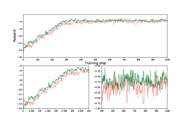
(a) Ant Push Multi

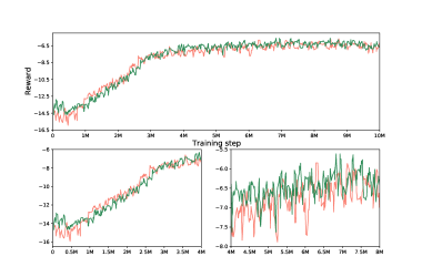
(b) Ant Fall Multi

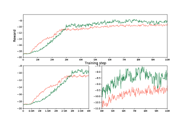
(c) Ant Push Single

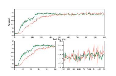
(d) Ant Fall Single

Figure 3: Average reward of our method(green) compared with that of HIRO with the same size (orange)

IV-C Off-policy correction

To overcome the disadvantage of the on-policy RL where the policy may be trapped in local minima, the off-policy RL, where an update policy is different from a behaviour policy has become an area of great interest. However, the off-policy method in HRL has a non-stationary issue. If a goal-conditioned HRL is trained in bottom-up training, a previously used output, i.e. a goal, of the higher-level policy may not be appropriate for training since it does not reflect the value of the parameter $\theta$ of the trained lower-level policy.

Let’s assume the operation of a lower policy $\mu^{lo}$ of a HRL,

$$a_{t}\sim\mu_{\theta}^{lo}(s_{t},g_{t}),\text{ at time}\leavevmode\nobreak\ t,$$

where $a_{t}$ is the action of $\mu^{lo}$ at time t, $s_{t}$ is the state of environment at time t, $g_{t}$ is the goal at time t which is the action of the higher-level policy $\mu^{hi}$. After $\mu_{\theta}^{lo}$ is trained after c steps,

$$a_{t+c}\sim\mu_{\theta^{\prime}}^{lo}(s_{t+c},g_{t}) s_{t+c}=s_{t}$$ , assume

$$a_{t}\neq a_{t+c}{}\,\text{or} \,a_{t}=a_{t+c}$$

where $a_{t+c}$ and $s_{t+c}$ are the action of $\mu_{\theta^{\prime}}^{lo}$ and the state of the environment after c steps respectively. $a_{t+c}$ may not be the same as $a_{t}$ for the value of the $\mu_{\theta}^{lo}$ parameter which might be different from that of the $\mu_{\theta^{\prime}}^{lo}$ parameter.

A replay buffer collected by a higher-level policy for the off-policy RL is filled with state-action-reward transitions ($s_{t}$, $g_{t}$, $a_{t,z}$, $a_{t,z-state}$, $a_{t,rnvp}$, $\Sigma{R_{t:t+c-1}}$, $s_{t+c}$) based on a higher-level transition tuple $(s_{t:t+c-1}$, $g_{t:t+c-1}$, $a_{t:t+c-1,z}$, $a_{t:t+c-1,z-state}$, $a_{t:t+c-1,rnvp}$, $R_{t:t+c-1}$, $s_{t+c})$.

When the higher-level policy is trained, the inverse operation of FDGM of its lower-level policy is executed by

$$\tilde{g}_{t}\sim\mu_{lo,FDGM}^{-1}(a_{t,rnvp},a_{t,z-state})$$

with $a_{t,rnvp}$, $a_{t,z-state}$ taken from the replay buffer. To relabel $g_{t}$, $\tilde{g}_{t}$ is utilized when the higher-level policy is trained after the lower-level policy is trained in a bottom-up layer-wise fashion which is followed in our research.

Our research takes advantage of TD3 on every policy. TD3 has an actor-critic structure where it causes a burden to balance the width size of a layer of both RealNVP which is used in the actor of FDGM and a fully connected neural network which is used in all policies including the critic of FDGM. In addition, the dynamic of the inverse operation using our inverse model for the best performance has been different for each task of the environment. Thus, we propose Algorithm 1 and Algorithm 2 to find an optimal goal for the off-policy correction using our inverse model. Algorithm 2 is used only for the Ant Fall Single task.

V Experiments

In this research, we investigate whether our inverse model in HRL using the direct method with FDGM for off-policy correction can achieve competitive performance against HIRO. Hence, to achieve the main purpose of the experiment, we only made two modifications to the open program of HIRO, namely to replace the neural network of the lower-level policy of HIRO with the architecture of our model and to use the inverse operation of our model, Algorithm 1 or Algorithm 2, instead of the probabilistic method of HIRO. All the remaining parts are unchanged. This makes it easy to compare the performance of our model with HIRO.

We are also interested in the variant of our model architecture since it shows the importance of the conditional part. If one input of the conditional part, $a_{t,z}$, is replaced by a goal $g_{t}$, it provides more goal components in the FDGM part so that we can determine whether or not it shows the importance of a $a_{t,z}$ as well as a goal $g_{t}$ for the inverse operation of the FDGM part.

Finally, our research and the variant of our research is compared with HIRO in terms of the average reward result of the higher-level policy based on the same environment as HIRO. HIRO was used in the tasks of the Mujoco ant environment of the OpenAI Gym, Ant Push Multi, Ant Fall Multi, Ant Push Single and Ant Fall Single to evaluate the performance of our research. The detail of the experiment is in Appendix A.

The objectives of our experiments are as follows:

1)	To verify that our inverse model improves the performance of the agent more than HIRO
2)	To prove that the variant of our model changes the performance of the agent more than our original model
3)	To evaluate how much the performance of our model is different in each task in terms of the availability of our inverse model
4)	To evaluate to what degree our algorithm addresses the chronic issue of FDGM in HRL

V-A Comparative analysis

For the comparison with HIRO, first we find the appropriate parameters for our model to achieve the best performance in each task. Then, using the same parameters, the performance of HIRO was compared with our model for each task.

In all the tasks, the widths of all the neural networks of each policy are fine-tuned. In addition, the dimension of $a_{t,z-state}$ of the conditional part is also tuned. The fine-tuning process aims to find the optimal $\tilde{g}_{t}$ from the FDGM part reflecting the current state of the lower-level policy in each task. Algorithm 1 and 2 calculate the fine-tuning process for each task in the experiment. In Fig. 3, the average results of our model for the tasks of the higher-level policy are compared with those of HIRO with the same parameters as our model.

Ant Push Multi (Actor of FDMG : 145, All other NNs : 170, $a_{t,z-state}$ = 16) in Fig. 3(a): We achieved better scores than HIRO with the same parameters until 4.5M. Then our results marginally outperformed HIRO up to 10M.

Ant Fall Multi (Actor of FDMG : 150, All other NNs : 170, $a_{t,z-state}$ = 18) in Fig. 3(b): Our model and HIRO with the same parameters achieved similar results until 4.8M. Then, the performance of our model was slightly better up to 8M.

Ant Push Single (Actor of FDMG : 130, All other NNs : 150, $a_{t,z-state}$ = 19) in Fig. 3(c): Our model achieved considerably better performance until 10M than HIRO with the same parameters although our model’s result was not as good as HIRO’s up to 3M.

Ant Fall Single (All lower policy’s NNs : 135, All higher policy’s NNs : 160, $a_{t,z-state}$ = 24) in Fig. 3(d): Our model achieved a much higher speed of learning up to 5.25M than HIRO with the same parameters. Our result was similar to HIRO’s up to 8M, after which it was slightly lower until 10M.

V-B Ablation study

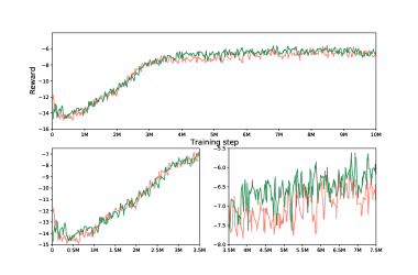
Figure 4: Average result of our method (green) compared with that of the variant model (orange) in Ant Fall Multi

The importance of $a_{t,z}$ attracts our interest because it plays a role in dealing with the chronic issue of FDGM, which is a biased log-density issue. If it is replaced by goal $g_{t}$ instead of $a_{t,z}$ for the input of the conditional part, it would be interesting to see how much the performance of our model changes.

Ant Fall Multi of variant model (Actor of FDMG : 150, All other NNs : 180, $a_{t,z-state}$ = 19): In this experiment, we did not set the size of the neural network of each policy to be the same as that of our model in the comparative analysis. The parameters of the variant model again resulted in the best performance. The performance of our original model in the Ant Fall Multi experiment of the comparative analysis was compared with the variant model with the newly found parameters. This shows that although both experiments resulted in the same performance until 3.5M, our original model marginally outperformed it up to 7.5M. Then, our original model and the variant model again performed the same up to 10M. The performance of our model against the variant model is shown in Fig. 4.

VI Discussion

VI-A The performance of the higher-level policy based on our model in all tasks

In all 4 tasks of the experiments, our model outperforms HIRO. Even though we do not use any indirect method such as a probabilistic method of HIRO, our model achieves competitive performance against HIRO by only using the inverse operation of FDMG. In particular, the lower-level policy which comprises three neural networks does not affect the performance of the early learning stage of the higher-level policy. Since the dimension of $a_{t,z-state}$ and the width size of each neural network of both level policies has an effect on the performance of a higher-level policy, their fine-tuning is required.

VI-B The different width size of the actor of the FDMG part in Algorithm 1

The reason why Algorithm 1 and 2 are considered is because of the level and speed of performance of the higher-level policy, respectively. Since our model takes advantage of TD3 in a policy, the FDMG part also has a combination of actor and critic. Interestingly, if the width of the actor is the same as the size of all other neural networks in Algorithm 1, the performance of the higher-level policy cannot reach our expectation. When there is a difference in the width size of neural network between that of the actor of FDMG and those of all other neural network to some degree, the anticipated performance is ensured.

VI-C The performance difference between the low reward shape and the high reward shape

Even though our model achieved better performance than HIRO for all tasks, there was a difference in the performance between the high reward shape of Ant Push Multi and Ant Fall Multi and the low reward shape of Ant Push Single and Ant Fall Single. This is likely due to the following two reasons. One is that the chronic issue of FDMG, i.e. biased log-density estimation, still affects the inverse operation of the FDMG. In particular, RealNVP used in our implementation is the early version of FDGM. The second reason is that the size of the data used in our experiment is much smaller than that of the image data utilized in [36], which affects the performance of our model. The former reason is more important than the latter.

VII Conclusion

We have presented a novel HRL inverse model which supports the level synchronization method using FDGM for the off-policy correction of HRL. Our model is superior to HIRO as shown in the results of the four test tasks of the Ant environment which is composed of two reward shapes, namely a high reward shape and a low reward shape. Our model demonstrates the general method for the inverse model of the model-free RL in HRL.

Our research proves that the off-policy correction in HRL can be implemented with the data acquired from a neural network such as FDGM. It is a more reasonable and generally applicable approach having a natural data computation without the knowledge of any peripheral information.

To date, there has been scant research on FDGM in the RL area. Usually, most RL research takes advantage of a general neural network such as a fully connected neural network. As an RL may require a further function such as the inverse operation, it is necessary for more RL research to be undertaken in the future using a generative model.

We also note that further research is required to improve our model. Further research on RL should be conducted using a general FDGM algorithm, not to investigate data which is massive in size such as images, but rather, data which is small in size such as the feature space used in RL.

Appendix A Experiment details

Our implementation is based on HIRO open code and RealNVP in [8]. We have released our code with explanations . The definition of a goal and the intrinsic reward function of a lower-level policy defined in HIRO are used without modification. Only the implementation of the lower-level policy and off-policy correction of the HIRO open code has been changed. In addition, the implementation of RealNVP in [8] is adopted to the HIRO open code. The two-level hierarchical structure of HRL is used because the same HRL structure of HIRO is used. In the Ant environment, the dimension of state $s_{t}$ and action $a_{t,z}$ is 30 and 8, respectively. The main parameters which are defined in our model for all tasks are the same as those for HIRO. The dimension of goal $g_{t}$ is 15. The default width size of the two hidden layers of a policy is 300 for both policies. The evaluation step used in this research is 10M steps. All the other training parameters are the same as those for HIRO. On the other hand, all other neural networks including the critic of the FDGM part except for the actor of the FDGM part, which is a RealNVP, consist of a fully connected neural network as utilized in HIRO. When our model is compared with HIRO with the same parameters, the size of the higher-level policy and lower-level policy of HIRO is defined according to Algorithm 1 or 2. Particularly in Algorithm 1, the width size of the lower-level policy of HIRO with the same parameters is the same as that of the actor of the FDGM part of our model.

JaeYoon Kim is currently a PhD student in the University of Technology Sydney. He is interested in researching Reinforcement Learning, especially Hierarchical RL, Transfer RL and Model-Based RL.

Junyu Xuan (Member, IEEE) is currently a Senior Lecturer with the Australian Artificial Intelligence Institute, University of Technology Sydney, Ultimo, NSW, Australia. He has authored or coauthored more than 40 articles in high-quality journals and conferences, including Artificial Intelligence, Machine Learning, TNNLS, the ACM Computing Surveys, TKDE, TOIS, and TCYB. His main research interests include Bayesian nonparametric learning, text mining, and web mining.

Christy Liang Christy Jie Liang is a senior lecturer whose research interests focus on data visualisation and visual analytics science technology. She leads the data visualization research lab in the Visualization Institute, University of Technology Sydney. She owns 4 intellectual properties and has published more than 40 articles in top tier venues in the visualisation research field.

Farookh Hussain (Member, IEEE) Associate Professor Farookh Hussain is a NSW Council member of the Australian Information Industry Association (AIIA). He is an AI and image processing researcher with the Decision Systems and e-Service Intelligence Lab at the Australian Artificial Intelligence Institute and Head of Discipline (Software Engineering) at the School of Computer Science in the UTS Faculty of Engineering and Information Technology.

References

- [1] R. S. Sutton and A. G. Barto, Reinforcement learning: An introduction. MIT press, 2018.
- [2] D. Silver, G. Lever, N. Heess, T. Degris, D. Wierstra, and M. Riedmiller, “Deterministic policy gradient algorithms,” in International conference on machine learning. PMLR, 2014, pp. 387–395.
- [3] V. Mnih, K. Kavukcuoglu, D. Silver, A. Graves, I. Antonoglou, D. Wierstra, and M. Riedmiller, “Playing atari with deep reinforcement learning,” arXiv preprint arXiv:1312.5602, 2013.
- [4] T. P. Lillicrap, J. J. Hunt, A. Pritzel, N. Heess, T. Erez, Y. Tassa, D. Silver, and D. Wierstra, “Continuous control with deep reinforcement learning,” arXiv preprint arXiv:1509.02971, 2015.
- [5] T. Haarnoja, A. Zhou, P. Abbeel, and S. Levine, “Soft actor-critic: Off-policy maximum entropy deep reinforcement learning with a stochastic actor,” in International Conference on Machine Learning. PMLR, 2018, pp. 1861–1870.
- [6] S. Fujimoto, H. Hoof, and D. Meger, “Addressing function approximation error in actor-critic methods,” in International Conference on Machine Learning. PMLR, 2018, pp. 1587–1596.
- [7] O. Nachum, S. Gu, H. Lee, and S. Levine, “Data-efficient hierarchical reinforcement learning,” arXiv preprint arXiv:1805.08296, 2018.
- [8] T. Haarnoja, K. Hartikainen, P. Abbeel, and S. Levine, “Latent space policies for hierarchical reinforcement learning,” in International Conference on Machine Learning. PMLR, 2018, pp. 1851–1860.
- [9] J. Rafati and D. C. Noelle, “Learning representations in model-free hierarchical reinforcement learning,” in Proceedings of the AAAI Conference on Artificial Intelligence, vol. 33, no. 01, 2019, pp. 10 009–10 010.
- [10] T. Osa, V. Tangkaratt, and M. Sugiyama, “Hierarchical reinforcement learning via advantage-weighted information maximization,” arXiv preprint arXiv:1901.01365, 2019.
- [11] J. Co-Reyes, Y. Liu, A. Gupta, B. Eysenbach, P. Abbeel, and S. Levine, “Self-consistent trajectory autoencoder: Hierarchical reinforcement learning with trajectory embeddings,” in International Conference on Machine Learning. PMLR, 2018, pp. 1009–1018.
- [12] T. Degris, M. White, and R. S. Sutton, “Off-policy actor-critic,” arXiv preprint arXiv:1205.4839, 2012.
- [13] P.-L. Bacon, J. Harb, and D. Precup, “The option-critic architecture,” in Proceedings of the AAAI Conference on Artificial Intelligence, vol. 31, no. 1, 2017.
- [14] V. Mnih, J. Agapiou, S. Osindero, A. Graves, O. Vinyals, K. Kavukcuoglu et al., “Strategic attentive writer for learning macro-actions,” arXiv preprint arXiv:1606.04695, 2016.
- [15] A. S. Vezhnevets, S. Osindero, T. Schaul, N. Heess, M. Jaderberg, D. Silver, and K. Kavukcuoglu, “Feudal networks for hierarchical reinforcement learning,” in International Conference on Machine Learning. PMLR, 2017, pp. 3540–3549.
- [16] M. Andrychowicz, F. Wolski, A. Ray, J. Schneider, R. Fong, P. Welinder, B. McGrew, J. Tobin, P. Abbeel, and W. Zaremba, “Hindsight experience replay,” arXiv preprint arXiv:1707.01495, 2017.
- [17] A. Levy, R. Platt, and K. Saenko, “Hierarchical actor-critic,” arXiv preprint arXiv:1712.00948, vol. 12, 2017.
- [18] A. Levy, G. Konidaris, R. Platt, and K. Saenko, “Learning multi-level hierarchies with hindsight,” arXiv preprint arXiv:1712.00948, 2017.
- [19] O. Nachum, S. Gu, H. Lee, and S. Levine, “Near-optimal representation learning for hierarchical reinforcement learning,” arXiv preprint arXiv:1810.01257, 2018.
- [20] I. J. Goodfellow, J. Pouget-Abadie, M. Mirza, B. Xu, D. Warde-Farley, S. Ozair, A. Courville, and Y. Bengio, “Generative adversarial networks,” arXiv preprint arXiv:1406.2661, 2014.
- [21] D. P. Kingma and M. Welling, “Auto-encoding variational bayes,” arXiv preprint arXiv:1312.6114, 2013.
- [22] G. E. Hinton and R. R. Salakhutdinov, “Reducing the dimensionality of data with neural networks,” science, vol. 313, no. 5786, pp. 504–507, 2006.
- [23] A. Odena, C. Olah, and J. Shlens, “Conditional image synthesis with auxiliary classifier gans,” in International conference on machine learning. PMLR, 2017, pp. 2642–2651.
- [24] A. Radford, L. Metz, and S. Chintala, “Unsupervised representation learning with deep convolutional generative adversarial networks,” arXiv preprint arXiv:1511.06434, 2015.
- [25] X. Mao, Q. Li, H. Xie, R. Y. Lau, Z. Wang, and S. Paul Smolley, “Least squares generative adversarial networks,” in Proceedings of the IEEE international conference on computer vision, 2017, pp. 2794–2802.
- [26] J. Su and G. Wu, “f-vaes: Improve vaes with conditional flows,” arXiv preprint arXiv:1809.05861, 2018.
- [27] S. Kolouri, P. E. Pope, C. E. Martin, and G. K. Rohde, “Sliced-wasserstein autoencoder: An embarrassingly simple generative model,” arXiv preprint arXiv:1804.01947, 2018.
- [28] T. Rainforth, A. Kosiorek, T. A. Le, C. Maddison, M. Igl, F. Wood, and Y. W. Teh, “Tighter variational bounds are not necessarily better,” in International Conference on Machine Learning. PMLR, 2018, pp. 4277–4285.
- [29] I. Tolstikhin, O. Bousquet, S. Gelly, and B. Schoelkopf, “Wasserstein auto-encoders,” arXiv preprint arXiv: 1711.01558, 2017.
- [30] T. Salimans, I. Goodfellow, W. Zaremba, V. Cheung, A. Radford, and X. Chen, “Improved techniques for training gans,” arXiv preprint arXiv:1606.03498, 2016.
- [31] L. Dinh, J. Sohl-Dickstein, and S. Bengio, “Density estimation using real nvp,” arXiv preprint arXiv:1605.08803, 2016.
- [32] L. Dinh, D. Krueger, and Y. Bengio, “Nice: Non-linear independent components estimation,” arXiv preprint arXiv:1410.8516, 2014.
- [33] D. P. Kingma and P. Dhariwal, “Glow: Generative flow with invertible 1x1 convolutions,” arXiv preprint arXiv:1807.03039, 2018.
- [34] J. Ho, X. Chen, A. Srinivas, Y. Duan, and P. Abbeel, “Flow++: Improving flow-based generative models with variational dequantization and architecture design,” in International Conference on Machine Learning. PMLR, 2019, pp. 2722–2730.
- [35] R. T. Chen, J. Behrmann, D. Duvenaud, and J.-H. Jacobsen, “Residual flows for invertible generative modeling,” arXiv preprint arXiv:1906.02735, 2019.
- [36] X. Ma, X. Kong, S. Zhang, and E. Hovy, “Decoupling global and local representations from/for image generation,” arXiv preprint arXiv:2004.11820, 2020.
- [37] M. Germain, K. Gregor, I. Murray, and H. Larochelle, “Made: Masked autoencoder for distribution estimation,” in International Conference on Machine Learning. PMLR, 2015, pp. 881–889.
- [38] A. Van Oord, N. Kalchbrenner, and K. Kavukcuoglu, “Pixel recurrent neural networks,” in International Conference on Machine Learning. PMLR, 2016, pp. 1747–1756.
- [39] A. v. d. Oord, S. Dieleman, H. Zen, K. Simonyan, O. Vinyals, A. Graves, N. Kalchbrenner, A. Senior, and K. Kavukcuoglu, “Wavenet: A generative model for raw audio,” arXiv preprint arXiv:1609.03499, 2016.
- [40] G. Papamakarios, T. Pavlakou, and I. Murray, “Masked autoregressive flow for density estimation,” arXiv preprint arXiv:1705.07057, 2017.
- [41] D. P. Kingma, T. Salimans, R. Jozefowicz, X. Chen, I. Sutskever, and M. Welling, “Improving variational inference with inverse autoregressive flow,” arXiv preprint arXiv:1606.04934, 2016.