claimClaim remarkRemark hypothesisHypothesis explExample

Model
Uncertainty & Correctability for Graphical ModelsP. Birmpa, J. Feng, M. A. Katsoulakis, L. Rey-Bellet






Model Uncertainty and Correctability for Directed Graphical Models


Panagiota Birmpa
Department of Mathematics and Statistics, University of Massachusetts, Amherst, U.S.A ().
birmpa@math.umass.edu

  
Jinchao Feng
Department of Applied Mathematics and Statistics, Johns Hopkins University, Baltimore, U.S.A ().
jfeng34@jhu.edu

  
Markos A. Katsoulakis
Department of Mathematics and Statistics, University of Massachusetts, Amherst, U.S.A ().
markos@math.umass.edu

  
Luc Rey-Bellet
Department of Mathematics and Statistics, University of Massachusetts, Amherst, U.S.A ().
luc@math.umass.edu




Abstract
Probabilistic graphical models are a fundamental tool in probabilistic modeling, machine learning and artificial intelligence. They allow us to integrate in a natural way expert knowledge, physical modeling,
heterogeneous and correlated data and quantities of interest. For exactly this reason, multiple sources of model uncertainty are inherent within the modular structure of the graphical model. In this paper we develop information-theoretic, robust uncertainty quantification methods and non-parametric stress tests for directed graphical models to assess the effect and the propagation through the graph of multi-sourced model uncertainties to quantities of interest.
These methods allow us to rank the different sources of uncertainty and correct the graphical model by targeting its most impactful components with respect to the quantities of interest. Thus, from a machine learning perspective, we provide a mathematically rigorous approach to correctability that guarantees a systematic selection for improvement of
components of a graphical model while controlling potential new errors created in the process in other parts of the model.
We demonstrate our methods in two physico-chemical examples, namely quantum scale-informed chemical kinetics and materials screening to improve the efficiency of fuel cells.


keywords: 
Bayesian networks, uncertainty quantification, sensitivity analysis, stress tests, information inequalities, correctability



62H22, 62P30, 68T37, 80A30, 93B35, 94A17 




1 Introduction


Data-informed, structured probability models are typically constructed by combining expert-based mathematical models with available data, the latter often being heterogeneous, i.e. from multiple sources and scales, and possibly sparse or imperfect.
Typically such structured models are formulated as probabilistic graphical models (PGM), which in turn are generally classified into Markov Random Fields (MRFs) over undirected graphs and Bayesian Networks (Bayesian network) over Directed Acyclic Graph (DAG) [58, 48],
as well as mixtures of those two classes, [31]. In this paper we focus on Bayesian Networks. DAGs are graphs with directed edges and without cycles, where individual vertices correspond to different model components or data inputs, while the directed edges
encode
conditional dependencies between vertices.
Formally, a Bayesian Network over a DAG is defined as a pair $\{G,P\}$ consisting of the following ingredients: $G=\{V,E\}$ is a DAG with $n$ vertices denoted by $V=\{1,\dots,n\},n\in\mathbb{N}$, along with directed, connecting edges $E\in V\times V$. In addition, we define a set of random variables $X_{V}=\{X_{1},\dots,X_{n}\}$ over $V$ with probability distribution $P$ with density



(1)

$$p(x)=\prod_{i=1}^{n}p(x_{i}|x_{\pi_{i}})$$



where $x_{\pi_{i}}=\{x_{i_{1}},\dots,x_{i_{m}}\}\subset\{x_{1},\dots,x_{n}\}$ denotes the values of parents $\pi_{i}$ of each vertex $i$,
see Figure 1,
and
$p(x_{i}|x_{\pi_{i}})$
is the Conditional Probability Density (CPD) for the conditional distribution $P_{i|\pi_{i}}$ with parents $\pi_{i}$.
In such models we are typically interested in quantities of interest (QoI) $f(X_{A})$ that involve one or more vertices $A\subset V$ and the corresponding random variables $X_{A}\subset X_{V}$.


The general mathematical formulation of PGMs was developed in foundational works in [58, 59], and
are widely used in many real-world applications of Artificial Intelligence, like medical diagnostics, natural language processing, computer vision, robotics, computational biology, cognitive science to name a few, e.g., [27, 42, 3, 51, 50, 28].
Recently PGMs were built as computationally tractable surrogates for multi-scale/multi-physics models
(e.g. from quantum to molecular to engineering scales), such as in porous media and energy storage,
[69, 40]. Such models often have hidden correlations in data used in their construction [68] or include physical constraints in parameters [69], necessitating conditional relations between model components and thus giving rise to CPDs such as the ones in (1).
Finally, PGMs can be used as the mathematical foundation for building digital twins used for control and optimization tasks of real systems [61].
Some examples include Bayesian networks for fuel cells [26] and Hidden Markov models (a time-dependent special case of Bayesian networks)
for unmanned aerial vehicles [46].
The structured probabilistic nature of such models allows them to be continuously improved, e.g. based on available real-time data [46] or through targeted data acquisition [26].


A. Model Uncertainty in Bayesian networks.
Bayesian networks
will typically have multiple sources of uncertainty due to modeling choices or learning from imperfect data in the process of building the graph $G$ and each one of the CPDs in (1). These uncertainties will propagate (and occasionally not propagate – see Section 7) through the directed graph structure to the targeted QoIs.
Uncertainties in probabilistic models are broadly classified in two categories: aleatoric, due to the inherent stochasticity of probabilistic models such as (1)
and model uncertainties (also known as “epistemic”), [21, 65]. In this paper we primarily focus on model uncertainties which stem from the inability to accurately model one or more of the components of a Bayesian Network $\{G,P\}$: omitting or simplifying model components as is often the case in multi-scale systems, learning from sparse data, or using approximate inference methods to build CPDs in (1).
Next, we discuss more concretely these challenges in the context of two physico-chemical examples that we analyze further using model uncertainty methods developed here.



First, we consider a Langmuir bimolecular adsorption model (see Section 6) that describes the chemical kinetics with competitive dissociative adsorption of hydrogen and oxygen on a catalyst surface [62, 24]. It is a multi-scale system of random differential equations with correlated dependencies in their parameters (kinetic coefficients), arising from quantum-scale computational data calculated using Density Functional Theory (DFT) (i.e quantum computations) for actual metals. The combination of chemical kinetics with parameter dependencies, correlations and DFT data gives rise naturally to a Bayesian network. The QoIs are the equilibrium hydrogen and oxygen coverages computed as the stationary solutions of a system of mean-field differential equations.
Here the Bayesian network allows us to incorporate data and correlations from a different scale to the parameters of an established chemical kinetics (differential equations) model.
However, the limited availability of the quantum-scale data creates significant model uncertainties in the distributions of kinetic coefficients, see for example Figure 5(a), and the need to be accounted towards obtaining reliable predictions for the QoI.


In a second example analyzed in Section 7 we build suitable Bayesian networks for trustworthy screening of materials to increase the efficiency of chemical reactions. Here we consider the Oxygen Reduction Reaction (ORR) which is a known performance bottleneck in fuel cells [63]. This electrochemistry mechanism involves two reactions which are typically slow. Thus, we seek new materials that speed up these two slowest reactions. For this reason here we focus only on the thermodynamics of these reactions described by the volcano curve of the Sabatier’s principle [62].
Based on the Sabatier’s principle, the optimal oxygen binding energy is the natural descriptor for discovering new materials and hence it has to be our QoI. Starting from this QoI we build a Bayesian network that includes expert knowledge (volcano curves), as well as various available experimental and computational data and their correlations or conditional independence.
Model uncertainties enter in the construction of the Bayesian network due to lack of complete knowledge of physics and sparse, expensive, multi-sourced experimental and/or computational data, see for example Figure 7(c-g).


Both these examples illustrate how PGMs (here Bayesian networks) allow to (a) organize in a natural way expert knowledge, modeling, heterogeneous and correlated data and QoIs; (b) study the propagation of all related model uncertainties to the QoI through the graph.
Practically these PGMs are built around the QoI so that it contains all available sources of information that may influence QoI predictions.


B. Mathematical results.
In this article we focus on quantifying model uncertainties in Bayesian networks.
Due to the graph structure of the models such uncertainties can be localized and their propagation to the QoI is affected by the graph and the CPDs in (1).
We develop model uncertainty and model sensitivity indices to quantify their impact, taking advantage of the graph structure.


First, we refer to an already constructed Bayesian network $\{G,P\}$ as the baseline model. We will describe mathematically the model uncertainty of the baseline by considering alternative models $Q$ in a suitably defined neighborhood of $P$ referred to as the ambiguity set,



(2)

$$\mathcal{D}^{\eta}:=\{\textrm{all Bayesian networks }Q:d(Q,P)\leq\eta\}\,.$$



The two primary ingredients for constructing ambiguity sets are the choice of a divergence or probabilistic metric $d$ between the baseline Bayesian network $P$ and an alternative model $Q$ and its size $\eta$ called model misspecification which essentially describes the level of uncertainty in the model.
Next, given an ambiguity set $\mathcal{D}^{\eta}$, we define the model uncertainty indices for our QoI $f$ as



(3)

$$I^{\pm}(f,P;\mathcal{D}^{\eta}):=\underset{Q\in\mathcal{D}^{\eta}}{\mathrm{sup/inf}}\ \{\mathbb{E}_{Q}\left[f\right]-\mathbb{E}_{P}\left[f\right]\}\,.$$



We view these indices as a non-parametric stress test on the the baseline $P$ for the QoI $f$ within the ambiguity set $\mathcal{D}^{\eta}$,
since they provide the corresponding worst case scenarios. Furthermore, the ambiguity set is non-parametric, allowing us to test the robustness of
the baseline against a broader set of scenarios than just a fixed parametric family.


Here we will define ambiguity sets using the Kullback-Leibler (KL) divergence as it allows us to obtain
easily computable and scalable model uncertainty indices $I^{\pm}(f,P;\mathcal{D}^{\eta})$. Indeed, the KL chain rule allows us to break
down the calculation of any KL distance between different Bayesian network components, i.e. in terms of
conditional KL divergences between distinct CPDs as well as to isolate the uncertainty impact on QoIs from multiple Bayesian network components
and data sources. A discussion on other natural choices of divergences and metrics can be found in Section 8.
On the other hand, the model misspecification $\eta$ can be selected in two ways. First, by the user adjusting the stress test on the QoI, for example when available data are too sparse or absent.
Otherwise, $\eta$ can be estimated as the KL divergence between the model and the available data.
Thus, we can consider user-determined or data-informed stress tests respectively.


Next, we design different stress tests by adjusting the ambiguity set (2) to account for global or local perturbations/uncertainties of the baseline model (1).


Model uncertainty indices (perturbing the entire model).
Let $f(X_{A})$ be a QoI defined on any set of random variables $X_{A}\subset X_{V}$. The ambiguity set (2) in this case contains all the possible alternative Bayesian networks $Q$ $\eta$-close to the baseline Bayesian network $P$ in the KL divergence for some model misspecification $\eta$. In Theorem 2.1, we demonstrate that the model uncertainty indices for $f(X_{A})$ (3) can be re-written only in terms of the baseline $P$ through the one-dimensional optimization



(4)

$$I^{\pm}(f(X_{A}),P;\mathcal{D}^{\eta})=\pm\inf_{c>0}\Big{[}\frac{1}{c}\log\mathbb{E}_{P_{A}}\left[e^{\pm c\bar{f}(X_{A})}\right]+\frac{\eta}{c}\Big{]}=\mathbb{E}_{Q^{\pm}}\left[f\right]-\mathbb{E}_{P}\left[f\right]$$



where $P_{A}$ is the marginal distribution of $X_{A}$ and $\bar{f}(X_{A})$ is the centered QoI with respect to $P$. Furthermore, there exist optimizers $Q^{\pm}$ (last equality in (4)) that are Bayesian networks that can be computed explicitly. We note that although the optimization in (3) is infinite-dimensional and thus essentially computationally intractable, the formula (4) gives rise to a computable one-dimensional optimization involving only the baseline Bayesian network $P$. This significant advantage will be exploited throughout the paper to provide practical quantification of model uncertainty and model sensitivity for PGMs.


Next we quantify the robustness of the baseline against perturbations of individual components of (1). We intend to use
these methods to explore the relative sensitivity of the baseline on different Bayesian network components, hence we will refer to the corresponding
indices
model sensitivity indices.


Model sensitivity indices (Perturbing a model component).
Let $f(X_{k})$ be a QoI with $k\in V$. We examine two ambiguity sets depending on the manner individual model components are perturbed.
The first ambiguity set consists of all Bayesian networks (1) with the same CPDs except for the CPD at a specific vertex $l\in V$; the structure/parents of the component $l$ can be different, however the alternative CPDs are $\eta_{l}$-“close” to $P$ at the $l$-th component in KL divergence for some model misspecification $\eta_{l}$, see Figure 2.
The second ambiguity set consists of all Bayesian networks with the parents of the vertex $l$ being fixed and only the CPD of $l$ varying. Even if the latter set is a subset of the first ambiguity set, such graph-based constraints allow us to focus on uncertainties arising from a given CPD of the network. For these ambiguity sets, we derive explicit formulas for the corresponding sensitivity indices
that are tight and practically computable similarly to (4), see Theorem 3.2 and 3.4.


C. Model sensitivity for ranking and correctability.
Model sensitivity indices are used here to rank the impact of different sources of uncertainty, from least to most influential, in the prediction of QoIs for Bayesian networks.
From a machine learning perspective, such rankings are a systematic form of interpretability, i.e. the ability to identify cause and effect in a model, [19, 52, 13], and explainability, i.e. the ability to explain model outputs through the modeling and data choices made in the construction of the baseline predictive model, see [1] and references therein. In the ORR model discussed earlier,
we compute model misspecification parameters $\eta_{l}$ from data,
we implement the ranking procedure
for each graph component of the ORR Bayesian network (i.e solvation, DFT, experiment and parameter correlation) and reveal the least and the most influential parts of the Bayesian Network in the prediction of the optimal oxygen binding energy QoI,
see Figure 9 and Section 7.


Lastly we leverage model uncertainty and model sensitivity indices to improve the baseline with either targeted data acquisition or improved modeling of CPDs and graph $G$ in (1). We target for correction under-performing components of the baseline, i.e. those inducing the most uncertainty on the QoI in the ranking above. Again from a machine learning perspective such a strategy is a step towards the correctability of PGMs,
namely the ability to correct targeted components of a (baseline) model without creating new errors in other parts of the model in the process [1]. Indeed, in the ORR model, we correct the baseline Bayesian network in two distinct ways: by including targeted high quality data and by increasing the model complexity, e.g. considering richer CPD classes or more complex PGMs, as discussed in Section 7.
This is an example of closing the “data-model-predictions loop” by iteratively improving the model while taking into account trade-offs between model complexity, data and predictive guarantees on QoIs.


D. Related work. The robust perspective in (3) for general probabilistic models is known in the Operations Research literature as Distributionally Robust Optimization (DRO) and includes different choices for divergences or metrics in (2), see for example [17, 33, 74, 44, 29, 49, 53, 75, 12].
Related work is also encountered in macroeconomics, we refer to the book Hansen and Sargent [41]. Stress testing via a DRO perspective has been developed in the context of insurance risk analysis in [11]. Finally, [57] and
[37] develop robust uncertainty quantification methods using different combinations of concentration inequalities and/or information divergences.
Regarding sensitivity analysis, we note that existing methods, e.g., gradient and ANOVA-based methods [65] are suitable for parametric uncertainties, and thus cannot handle model uncertainty. Furthermore, it is not immediately obvious how they can take advantage of the graphical structure in Bayesian networks such as conditional independence.
Here, our mathematical methods broadly rely on UQ information inequalities for QoIs of high-dimensional probabilistic models and stochastic processes
[15, 21, 39, 9, 8] (see also Appendix A). The mathematical novelty of our results lies on extending these earlier works on directed graphs by developing the proper model uncertainty and model sensitivity framework for general Bayesian networks and studying
the propagation of multiple uncertainties through the network to the QoIs.
Earlier work on building a predictive chemistry-based PGM with quantified model uncertainty for the resulting Gaussian Bayesian network was carried out in [26]
and demonstrated in materials design for speeding up the oxygen reduction reaction in fuel cells.
Model uncertainty for PGMs over undirected graphs, also known as Markov Random Fields (MRF) has been recently studied in [5]. An MRF is a unifying model for statistical mechanics (Gibbs measures) and machine learning (Boltzmann machines), while the special case of Gibbs measures was studied earlier in [47]. We note that for MRFs
the robust perspective is less flexible as we cannot fully take advantage of the KL chain rule due to the undirected structure of the graphs.


E. Organization. The main mathematical results are presented in Section 2 (model uncertainty) and Section 3 (model sensitivity).
In Section 4 and Section 5, we discuss ranking and correctability for Bayesian networks.
In Section 6 we discuss
a DFT-informed Langmuir model while
in Section 7 we analyze
the ORR model arising in fuel cells. In Section 8 we discuss some outstanding issues and directions.
Supporting material is included in the Appendices.



2 Model Uncertainty Indices for Bayesian networks


In this section, we develop model uncertainty methods and associated indices for Bayesian networks.
We start with the key ingredients needed to state and prove the main result (Theorem 2.1), namely the ambiguity set, QoIs and the definition of the model uncertainty indices.
First we define the ambiguity set
with model misspecification $\eta$ by



(5)

$$\mathcal{D}^{\eta}:=\{\textrm{all PGMs }Q:R(Q\|P)\leq\eta\}$$



where $R(Q\|P)=\mathbb{E}_{Q}\left[\log{\frac{dQ}{dP}}\right]$ denotes the KL divergence,
i.e. we perturb the baseline model $P$ to any alternative model $Q\in\mathcal{D}^{\eta}$, altering both the structure of the graph and the CPDs.


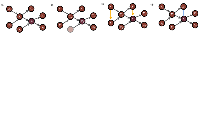
Figure 1: (a) Example of the graph structure of a baseline Bayesian network $P$ and the corresponding random variables $X=\{X_{1},\dots,X_{8}\}$. (b) Example of the graph structure of a Bayesian network $Q\in\mathcal{D}^{\eta}$ defined on a set with one vertex less than the baseline Bayesian network $P$. (c) An example of an alternative Bayesian network $Q\in\mathcal{D}^{\eta}$ with the same number of vertices while $X_{2}$ and $X_{8}$ have extra new parents (in yellow). (d) An example of a PGM $Q\in\mathcal{D}^{\eta}$ with a new undirected edge (in blue). 


Examples of models $Q$ included in $\mathcal{D}^{\eta}$ can be Bayesian networks defined on a smaller number of vertices than $P$, or same number of vertices with some of them having extra parents, or same number of vertices and parents but different CPDs, see Figure 1(b-c).
Furthermore, $\mathcal{D}^{\eta}$ can include PGMs which are not necessarily Bayesian networks, for example when some of the edges between vertices are not directed [31], see Figure 1(d). For a baseline Bayesian network $P$
we define the model uncertainty indices as




(6)

$$I^{\pm}(f(X_{A}),P;\mathcal{D}^{\eta})=\underset{Q\in\mathcal{D}^{\eta}}{\mathrm{sup/inf}}\ \mathbb{E}_{Q}\left[f(X_{A})\right]-\mathbb{E}_{P}\left[f(X_{A})\right]$$



for a QoI $f$ which is a function of some subset of $A$ vertices in the graph, i.e.,



(7)

$$\textrm{for }f(X_{A})=f(X_{i_{1}},\dots,X_{i_{m}}),\textrm{ with }A=\{i_{1},\dots,i_{m}\}\subseteq V\,.$$



In the next theorem, we characterize the optimizers $Q^{\pm}$ in (6) which turn out to be Bayesian networks of the form (1) and we provide their CPDs explicitly.


Notation. Before we state our results let us fix some notation. For a Bayesian network $\{G,P\}$
$\pi_{i}^{P}$ denotes the set of indices of all the parents of vertex $i$ and $\rho_{i}^{P}$ denotes the set of indices of all the ancestors for $i$ (we may omit the superscript “$P$” if only one Bayesian network is involved).
Without loss of generality we assume that all Bayesian networks are topologically ordered as we can always relabel the DAG so that $j<i$ for all $j\in\pi_{i}$ by topological sorting [48].


The random vector $X=(X_{1},\dots,X_{n})$, indexed by the vertices $V=\{1,...,n\}$, takes values $X=x=(x_{1},\dots,x_{n})\in\mathcal{X}$.
The joint probability distribution of $X$ is denoted by $P$ with density $p(x)$; the results are presented when the joint probability distribution $P$ is continuous but all results hold when $p$ is a discrete distribution as well. For any subset $A=\{i_{1},\cdots,i_{m}\}\subset V$ we denote $X_{A}=(X_{i_{1}},\cdots,X_{i_{m}})$ which takes values $X_{A}=x_{A}=(x_{i_{1}},\cdots,x_{i_{m}})\in\mathcal{X}_{A}$
and we denote by $P_{A}$ its marginal distribution.


We denote $P_{i|\pi_{i}^{P}}$ the conditional distribution of $X_{i}$ given parents values $X_{\pi_{i}^{P}}=x_{\pi_{i}}$, i.e. $P_{i|\pi_{i}^{P}}(dx_{i})=P(dx_{i}|x_{\pi_{i}})$ with corresponding CPD $p(x_{i}|x_{\pi_{i}})$.
The marginal distribution $P_{A}$ of $X_{A}$ has the form $P_{A}(dx_{A})=\int_{\mathcal{X}_{\rho_{A}}}\prod_{i\in A}P_{i|\pi_{i}^{P}}(dx_{i})\prod_{i\in\rho_{A}^{P}}P_{i|\pi_{i}^{P}}(dx_{i})$ where $\rho_{A}^{P}$ are the set of indices of all the ancestors of $A$, i.e. $\rho_{A}^{P}=\cup_{i\in A}\rho_{i}^{P}$. Furthermore the density $p_{A}$ of $P_{A}$ is
$p_{A}(x_{A})=\int_{\mathcal{X}_{\rho_{A}^{P}}}\prod_{i\in A}p(x_{i}|x_{\pi_{i}})\prod_{i\in\rho_{A}^{P}}p(x_{i}|x_{\pi_{i}})d{x_{\rho_{A}}}$.
Two special cases are the marginals of $X_{k}$, $P_{\{k\}}(dx_{k})=\int_{x_{\rho_{k}}}\prod_{i\in\{k\cup\rho_{k}\}}P(dx_{i}|x_{\pi_{i}})$ and the marginal of $X_{\rho_{A}}$, $P_{\rho_{A}}(dx_{\rho_{A}})=\prod_{i\in\rho_{A}}P(dx_{i}|x_{\pi_{i}})$.


Finally for $l_{1}<\cdots<l_{k}$ and any QoI $f$ and for $j\in\{1,\dots,k\}$ we define the notation



(8)

$$\mathbb{E}_{P_{l_{j}}|\pi_{l_{j}}^{P},\dots,P_{l_{k}}|\pi_{l_{k}}^{P}}[f]:=\mathbb{E}_{P_{l_{j}|\pi_{l_{j}}^{P}}}\left[\mathbb{E}_{P_{l_{j+1}|\pi_{l_{j+1}}^{P}}}\left[\cdots\mathbb{E}_{P_{l_{k}|\pi_{l_{k}}^{P}}}\left[f\right]\right]\right].$$






Theorem 2.1.


Let $\{G,P\}$ be a Bayesian network with density defined as (1), and $f(X_{A})$ be a QoI given in (7),
$f(X_{A})=f(X_{i_{1}},\dots,X_{i_{m}})$. Let also $\bar{f}(X_{A}):=f(X_{A})-\mathbb{E}_{P}\left[f(X_{A})\right]$ be the centered QoI with finite moment generating function (MGF), $\mathbb{E}_{P}\left[e^{c\bar{f}(X_{A})}\right]$, in a neighborhood of the origin.


$(a)$ Tightness. For the model uncertainty indices defined in (6), there exist $0<\eta_{\pm}\leq\infty$, such that for any $\eta\leq\eta_{\pm}$,




(9)

$$I^{\pm}(f(X_{A}),P;\mathcal{D}^{\eta})
=
\pm\inf_{c>0}\Big{[}\frac{1}{c}\log\mathbb{E}_{P_{A}}\left[\pm e^{c\bar{f}(X_{A})}\right]+\frac{\eta}{c}\Big{]}$$







$$=
\mathbb{E}_{Q^{\pm}}\left[f(X_{A})\right]-\mathbb{E}_{P}\left[f(X_{A})\right],$$





where $P_{A}$ is the marginal distribution of $X_{A}$ with respect to $P$, and $Q^{\pm}(\cdot)\equiv Q^{\pm}(\cdot\;;\pm c_{\pm})\in\mathcal{D}^{\eta}$ are Bayesian networks (1) that depend on $\eta$ and are given by



(10)

$$\frac{dQ^{\pm}}{dP}=\frac{e^{\pm c_{\pm}f(x_{A})}}{\mathbb{E}_{P}\left[e^{\pm c_{\pm}f(X_{A})}\right]}$$



where $c_{\pm}\equiv c_{\pm}(\eta)$ are the unique solutions of the equation



(11)

$$R(Q^{\pm}\|P)=\eta.$$





$(b)$ Graph Structure of $Q^{\pm}$. Let $L$ be all vertices that include $A$ and all its ancestors, i.e. $L=\underset{j\in A}{\cup}{\rho_{j}^{p}\cup A}=\{l_{1},\dots,l_{k+1}\}$, where $l_{1}<\cdots<l_{k+1}$ and $l_{k+1}=i_{m}$, then the CPDs of $Q^{\pm}$ are given by



(12)

$$q^{\pm}(x_{i}|x_{\pi_{i}^{Q^{\pm}}})=\begin{cases}p(x_{i}|x_{\pi_{i}^{P}})\,&\textrm{$i\notin L$}\\
\frac{\mathbb{E}_{P_{l_{j+1}}|\pi_{l_{j+1}}^{P},\dots,P_{l_{k}}|\pi_{l_{k}}^{P}}[e^{\pm c_{\pm}f(X_{A})}]}{\mathbb{E}_{P_{l_{j}}|\pi_{l_{j}}^{P},\dots,P_{l_{k}}|\pi_{l_{k}}^{P}}[e^{\pm c_{\pm}f(X_{A})}]}p(x_{l_{j}}|x_{\pi_{l_{j}}^{P}})\,&\textrm{$i=l_{j}$},\,j\in A\end{cases}$$



where $l_{j}\in L$ and $\mathbb{E}_{P_{l_{j}}|\pi_{l_{j}}^{P},\dots,P_{l_{k}}|\pi_{l_{k}}^{P}}$ is given by (8). The parents/structure is given by
$\pi_{i}^{Q^{\pm}}\equiv\pi_{i}^{P},i\notin L$ and $\pi_{l_{j}}^{P}\!\subset\!\pi_{l_{j}}^{Q^{\pm}}\!\subset\!\pi_{l_{j}}^{P}\!\cup\!(\pi_{l_{j+1}}^{Q^{\pm}}\setminus l_{j})$.



Remark 2.2.


Theorem 2.1 readily implies that we can severely restrict the ambiguity set (5) to a subclass of Bayesian networks, yielding the exact same index,



(13)

$$I^{\pm}(f(X_{A}),P;\mathcal{D}^{\eta})=I^{\pm}(f(X_{A}),P;\mathcal{D}^{\eta}_{\rho_{A}})$$



where a set of Bayesian networks $\mathcal{D}^{\eta}_{\rho_{A}}$ is defined as



(14)

$$\!\mathcal{D}^{\eta}_{\rho_{A}}:=\left\{\!\!\!\!\begin{array}[]{cc}\textrm{all Bayesian networks }Q:R(Q_{A\cup\rho_{A}}\|P_{A\cup\rho_{A}})\leq\eta\\
\textrm{ and }q(x_{i}|x_{\pi_{i}^{q}})\equiv p(x_{i}|x_{\pi_{i}^{p}})\ \textrm{with $\pi_{i}^{Q}\equiv\pi_{i}^{P}$ for all $i\notin A\cup\rho_{A}$}\end{array}\!\!\!\!\right\}.$$



This follows from the formula




$$\mathbb{E}_{P}\left[f(X_{A})\right]=\int_{\mathcal{X}}f(x_{A})\prod_{i=1}^{n}p(x_{i}|x_{\pi_{i}})dx=\int_{\mathcal{X}_{A\cup\rho_{A}}}f(x_{A})\prod_{x_{i}\in A\cup\rho_{A}}p(x_{i}|x_{\pi_{i}})dx_{A}dx_{\rho_{A}}$$



which implies that only the perturbation of $P_{A\cup\rho_{A}}$ affects the prediction of the QoI. A similar calculation for the MGF of $\bar{f}$
implies that the optimal $Q^{\pm}$ has the same CPDs as $P$ for all $X_{i}$, $i\notin\{A\}\cup\rho_{A}$, as shown in Theorem 2.1.





Remark 2.3.


We illustrate Theorem 2.1 in the special
case $A=\{k\}$, i.e QoIs defined on one vertex through the example in Figure 2, see also Appendix C for more details.


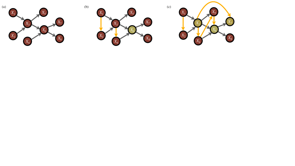
Figure 2: (a) Example of graph structure of a baseline Bayesian network $P$. (b) The structure of the optimizers $Q^{\pm}$ in Theorem 2.1 (b) with QoI $f(X_{6})$ is highlighted (in green). In contrast to the CPDs of the vertices involved in the QoI and their ancestors, the CPD of any other vertex does not change. The new parents of $X_{4},X_{2}$ are connected (in yellow), i.e. $X_{3}$ is a new parent for $X_{4}$ and $X_{1}$ is a new parent for $X_{2}$.
(c) Structure of the optimizers $Q^{\pm}$ in Theorem 2.1 (b) for a QoI of the type $f(X_{3},X_{6},X_{7})$, see (109)-(116). 










Proof of Theorem 2.1. $(a)$ The existence of $Q^{\pm}$ and (10) are direct consequences of (92) with $f(X)=f(X_{A})$. For $p(x)=\prod_{i=1}^{n}p(x_{i}|x_{\pi_{i}})$, we further compute




(15)

$$\underset{Q\in\mathcal{D}^{\eta}}{\mathrm{sup/inf}}\ \mathbb{E}_{Q}\left[f(X_{A})\right]-\mathbb{E}_{P}\left[f(X_{A})\right]
=
\pm\inf_{c>0}\Big{[}\frac{1}{c}\log\mathbb{E}_{P}\left[e^{\pm c\bar{f}(X_{A})}\right]+\frac{\eta}{c}\Big{]}$$







$$=
\pm\inf_{c>0}\Big{[}\frac{1}{c}\log\int_{\mathcal{X}}e^{\pm c\bar{f}(X_{A})}\prod_{i=1}^{n}P(dx_{i}|x_{\pi_{i}}^{P})+\frac{\eta}{c}\Big{]}$$






$$=
\pm\inf_{c>0}\Big{[}\frac{1}{c}\log\mathbb{E}_{P_{A}}\left[e^{\pm c\bar{f}(X_{A})}\right]+\frac{\eta}{c}\Big{]}$$





where $p_{A}$ is given in the notation before the theorem


$(b)$ We use (10) and we factorize $q^{\pm}$ as follows:




(16)

$$q^{\pm}(x)
=
\frac{e^{\pm c_{\pm}f(x_{A})}}{\mathbb{E}_{P}\left[e^{\pm c_{\pm}f(X_{A})}\right]}\prod_{i=1}^{n}p(x_{i}|x_{\pi_{i}^{P}})$$







$$=
\frac{1}{\mathbb{E}_{p_{A}}\left[e^{\pm c_{\pm}f(X_{A})}\right]}\prod_{i\notin\{l_{1},\dots,l_{k+1}\}}p(x_{i}|x_{\pi_{i}^{p}})\cdot e^{\pm c_{\pm}f(x_{A})}p(x_{i_{m}}|x_{\pi_{i_{m}}^{p}})$$







$$\quad\quad\times\prod_{i\in\{l_{1},\dots,l_{k}\}}p(x_{i}|x_{\pi_{i}^{p}})$$




where $\pm c_{\pm}$ are the unique solutions of $R(P^{\pm c_{\pm}}\|P)=\eta$. Formula (16) is not factorized yet into CPDs as in (1) due to the normalization factor at the denominator. The following analysis provides the steps for expressing (16) in a product of certain CPDs: Assuming that $i_{1}<\dots<i_{m}$, we start with the CPD of $X_{i_{m}}$ as its index is the largest among the elements of $A$. Based on (16),



(17)

$$q^{\pm}(x_{i_{m}}|x_{\pi_{i_{m}}^{q^{\pm}}})\propto e^{\pm c_{\pm}f(x_{A})}p(x_{i_{m}}|x_{\pi_{i_{m}}^{P}})$$



We normalize the LHS of (16) by dividing by



(18)

$$\mathbb{E}_{P_{i_{m}|\pi_{i_{m}}^{P}}}\left[e^{\pm c_{\pm}f(X_{A})}\right]$$



and by conditioning to $x_{\pi_{i_{m}}^{P}}$ and $x_{A\setminus i_{m}}$. Therefore, the CPD of $X_{i_{m}}$ and its parents $\pi_{i_{m}}^{Q^{\pm}}$ are given by




$$q^{\pm}(x_{i_{m}}|x_{\pi_{i_{m}}^{Q^{\pm}}})=\frac{e^{\pm c_{\pm}f(x_{A})}}{\mathbb{E}_{P_{i_{m}|\pi_{i_{m}}^{P}}}\left[e^{\pm c_{\pm}f(X_{A})}\right]}\cdot p(x_{i_{m}}|x_{\pi_{i_{m}}^{P}})\textrm{ and $\pi_{i_{m}}^{P}\subset\pi_{i_{m}}^{Q^{\pm}}=\pi_{i_{m}}^{P}\cup(A\setminus i_{m})$}$$



Such a consideration provides the new edges in the graph of $Q^{\pm}$. In particular, $X_{i_{m}}$ has the same parents as in $P$ model and possibly new parents specified by $x_{A\setminus i_{m}}$ e.g if $A\setminus i_{m}\neq\pi_{i_{m}}^{P}$. Next, we compute the CPD of $X_{l_{k}}$ since $l_{k}<l_{k+1}=i_{m}$: As we divided by (18) to normalize the the LHS of (16), we keep (16) same if we also multiple $q^{\pm}(x)$ by (18). Hence, we pair (16) and $p(x_{l_{k}}|x_{\pi_{l_{k}}^{P}})$ so as



(19)

$$q^{\pm}(x_{l_{k}}|x_{\pi_{l_{k}}^{Q^{\pm}}})\propto\mathbb{E}_{P_{i_{m}|\pi_{i_{m}}^{P}}}\left[e^{\pm c_{\pm}f(X_{A})}\right]p(x_{l_{k}}|x_{\pi_{l_{k}}^{P}})$$



As before, we normalize the LHS of (19) by dividing by



(20)

$$\mathbb{E}_{P_{l_{k}|\pi_{l_{k}}^{P}}}\left[\mathbb{E}_{P_{i_{m}|\pi_{i_{m}}^{P}}}\left[e^{\pm c_{\pm}f(X_{A})}\right]\right]$$



and by conditioning to $x_{\pi_{l_{k}}^{P}}$ and $x_{\pi_{i_{m}}^{Q^{\pm}}\setminus l_{k}}$, we obtain




$$q^{\pm}(x_{l_{k}}|x_{\pi_{l_{k}}^{Q^{\pm}}})=\frac{\mathbb{E}_{P_{i_{m}|\pi_{i_{m}}^{P}}}\left[e^{\pm c_{\pm}f(X_{A})}\right]}{\mathbb{E}_{P_{l_{k}|\pi_{l_{k}}^{p}}}\left[\mathbb{E}_{P_{i_{m}|\pi_{i_{m}}^{p}}}\left[e^{\pm c_{\pm}f(X_{A})}\right]\right]}\cdot p(x_{i_{m}}|x_{\pi_{i_{m}}^{P}})$$



and $\pi_{l_{k}}^{P}\subset\pi_{l_{k}}^{Q^{\pm}}=\pi_{l_{k}}^{P}\cup(\pi_{i_{m}}^{Q^{\pm}}\setminus l_{k})$. The latter shows the new edges that the associated graph to $Q^{\pm}$ may have. In this way, we obtain the remaining CPDs given by the second part of (12). It is straightforward that the random variables indexed differently than $\{l_{1},\dots,l_{k+1}\}$ inherent the corresponding CPDs of $P$, and thus (12) is obtained.



2.1 Gaussian Bayesian Networks


In this subsection, we focus on Gaussian Bayesian Networks. It is a special class of Bayesian networks commonly used in natural and social sciences with the CPDs as in (1)
being linear and Gaussian [48, 64, 35, 36, 34]. More specifically, for a Gaussian Bayesian network consisting of variables $X$, each vertex $X_{i}$ is a linear Gaussian of its parents, i.e.,



(21)

$$p(x_{i}|x_{\pi_{i}})=\mathcal{N}(\beta_{i0}+\beta_{i}^{T}x_{\pi_{i}},\sigma_{i}^{2}),\quad\textrm{ equivalently}$$




$$X_{i}=\beta_{i0}+\beta_{i}^{T}X_{\pi_{i}}+\epsilon_{i},\quad\textrm{ with }\epsilon_{i}\sim\mathcal{N}(0,\sigma_{i}^{2})$$



for some $\beta_{0}$, $\sigma_{i}$ and $\beta_{i}=[\beta_{ii_{1}},\dots,\beta_{ii_{|\pi_{i}|}}]$. By the conjugacy properties of Gaussians, the joint distribution $P$ becomes
$p(x)=\mathcal{N}(\mu,\mathcal{C})$, i.e. it
is also a Gaussian with parameters $\mu$, $\mathcal{C}$, which can be calculated from $\beta_{i0}$, $\beta_{i}$, and $\sigma_{i}$ [10].



Theorem 2.4.


Let $P$ be a Gaussian Bayesian network that satisfies (21), and $f(X_{k})=aX_{k}+b$ be a QoI only depends on $X_{k}$ linearly.


$(a)$ Then for the model uncertainty indices defined in (6), we have



(22)

$$I^{\pm}(f(X_{k}),P;\mathcal{D}^{\eta})=\pm\sqrt{2a^{2}\mathcal{C}_{kk}\eta}$$



where $\mathcal{C}_{kk}$ is the variance for the marginal distribution of $X_{k}$.


$(b)$ Furthermore, the optimizers $Q^{\pm}=Q^{\pm}(\eta)\in\mathcal{D}^{\eta}$ are given by (12) in Theorem 2.1 and are also Gaussian Bayesian networks with same graph structure as $P$.




Proof. (a) The distribution of $X_{k}$ denoted by $P_{\{k\}}$ is Gaussian with variance




$$\mathcal{C}_{kk}=\sigma_{k}^{2}+\beta_{k}^{T}\mathcal{C}_{\rho_{k}}\beta_{k}$$



where $\mathcal{C}_{\rho_{k}}$ is the variance of the joint distribution of the random variables $\{X_{i}:i\in\rho_{k}\}$, [48, Theorem 7.3]. By a straightforward computation, the moment generating function of $\bar{f}(X_{k})$ is given by




$$\mathbb{E}_{P_{\{k\}}}\left[e^{\pm c\bar{f}(X_{k})}\right]=\exp(a^{2}c^{2}\beta_{k}^{T}\mathcal{C}_{\rho_{k}}\beta_{k})$$







$$I^{\pm}(f(X_{k}),P;\mathcal{D}^{\eta})=\pm\inf_{c>0}\Big{[}\frac{1}{c}\log\mathbb{E}_{P_{\{k\}}}\left[e^{\pm c\bar{f}(X_{k})}\right]+\frac{\eta}{c}\Big{]}=\pm\inf_{c>0}\Big{[}a^{2}c\,\mathcal{C}_{kk}+\frac{\eta}{c}\Big{]}$$



Then, the optimal $c$ is given by $c=\sqrt{\frac{\eta}{a^{2}\mathcal{C}_{kk}}}$ which in turn proves (22).


(b) Next, we show that the graph structure of the $Q^{\pm}$ is the same as $P$. For any $j>k$, by Theorem 2.1, $q(x_{j}|x_{\pi_{j}^{Q^{\pm}}})=p(x_{j}|x_{\pi_{j}^{P}})$. For $j=k$, we compute





$$q^{\pm}(x_{k}|x_{\pi_{k}^{Q^{\pm}}})
=
\frac{e^{\pm c_{\pm}f(x_{k})}}{\mathbb{E}_{P_{k|\pi_{k}^{P}}}\left[e^{\pm c_{\pm}f(X_{k})}\right]}\cdot p(x_{k}|x_{\pi_{k}^{P}})$$







$$=
\frac{\exp\left\{-\frac{(x_{k}-\beta_{k0}-\beta_{k}^{T}x_{\pi_{k}^{P}}\mp c_{\pm}a\sigma_{k}^{2})^{2}}{2\sigma_{k}^{2}}\pm c_{\pm}a(\beta_{k}^{T}x_{\pi_{k}^{P}})\right\}}{\int_{\mathcal{X}_{k}}\exp\left\{-\frac{(x_{k}-\beta_{k0}-\beta_{k}^{T}x_{\pi_{k}^{P}}\mp c_{\pm}a\sigma_{k}^{2})^{2}}{2\sigma_{k}^{2}}\pm c_{\pm}a(\beta_{k}^{T}x_{\pi_{k}^{P}})\right\}dx_{k}}$$






$$=
\mathcal{N}\left(\beta_{k0}+\beta_{k}^{T}x_{\pi_{k}^{P}}\pm c_{\pm}a\sigma_{k}^{2},\sigma_{k}^{2}\right)$$





Thus $\pi_{k}^{Q^{\pm}}=\pi_{k}^{P}$ since $c_{\pm}a(\beta_{k}^{T}x_{\pi_{k}})$ of the numerator and denominator are canceled out. Let $k_{m}$ be the maximum element of $\pi_{k}^{P}=\{k_{1},\dots,k_{m}:k_{1}<\dots<k_{m-1}<k_{m}\}$ and $\beta_{k}^{m-1}:=[\beta_{kk_{1}},\dots,\beta_{kk_{m-1}}]$. Then



(25)

$$\;\;\;\;\;\;\;\;\;\;\;q^{\pm}(x_{k_{m}}|x_{\pi_{k_{m}}^{Q^{\pm}}})=\frac{\mathbb{E}_{P_{k|\pi_{k}^{P}}}\left[e^{\pm c_{\pm}f(X_{k})}\right]}{\mathbb{E}_{P_{k_{m}|\pi_{k_{m}}^{P}}}\left[\mathbb{E}_{P_{k|\pi_{k}^{P}}}\left[e^{\pm c_{\pm}f(X_{k})}\right]\right]}\cdot p(x_{k_{m}}|x_{\pi_{k_{m}}^{P}})$$




$$\qquad\;\;=\frac{\exp\left\{\pm c_{\pm}a\beta_{k}^{T}x_{\pi_{k}^{P}}-\frac{(x_{k_{m}}-\beta_{k_{m}0}-\beta_{k_{m}}^{T}x_{\pi_{k_{m}}^{P}})^{2}}{2\sigma_{m}^{2}}\right\}}{\int_{\mathcal{X}_{k_{m}}}\exp\left\{\pm c_{\pm}a\beta_{k}^{T}x_{\pi_{k}^{P}}-\frac{(x_{k_{m}}-\beta_{{k_{m}}0}-\beta_{k_{m}}^{T}x_{\pi_{k_{m}}^{P}})^{2}}{2\sigma_{k_{m}}^{2}}\right\}dx_{k_{m}}}$$




$$\qquad\;\;=\frac{\exp\left\{\pm c_{\pm}a(\beta_{k}^{m-1})^{T}x_{\pi_{k}^{P}\setminus k_{m}}-\frac{(x_{k_{m}}-\beta_{{k_{m}}0}-\beta_{k_{m}}^{T}x_{\pi_{k_{m}}^{P}}\mp c_{\pm}a\beta_{kk_{m}}\sigma_{k_{m}}^{2})^{2}}{2\sigma_{k_{m}}^{2}}\right\}}{\int_{\mathcal{X}_{k_{m}}}\exp\left\{\pm c_{\pm}a(\beta_{k}^{m-1})^{T}x_{\pi_{k}^{P}\setminus k_{m}}-\frac{(x_{k_{m}}-\beta_{{k_{m}}0}-\beta_{k_{m}}^{T}x_{\pi_{k_{m}}^{P}}\mp c_{\pm}a\beta_{kk_{m}}\sigma_{k_{m}}^{2})^{2}}{2\sigma_{k_{m}}^{2}}\right\}dx_{k_{m}}}$$




$$\qquad\;\;=\mathcal{N}\left(\beta_{{k_{m}}0}+\beta_{k_{m}}^{T}x_{\pi_{k_{m}}^{P}}\pm c_{\pm}a\beta_{kk_{m}}\sigma_{k_{m}}^{2},\sigma_{k_{m}}^{2}\right)$$



Again, $\pi_{k_{m}}^{Q^{\pm}}=\pi_{k_{m}}^{P}$ as the factor $\exp\left\{\pm c_{\pm}a(\beta_{k}^{m-1})^{T}x_{\pi_{k}^{P}\setminus k_{m}}\right\}$ in the numerator and denominator are canceled out. The CPD of the remaining vertices in $\pi_{k}^{P}$ are computed in the same way which further implies that their parents do not change. Therefore, the factors in CPDs of $Q^{\pm}$ that could create new directed edges appear in both numerator and denominator and are finally canceled out. We demonstrate (2.1) and (25) as it applies in Example C in Appendix C.



3 Model Sensitivity Indices for Bayesian networks


In this section, we develop a non-parametric sensitivity analysis for Bayesian networks by refining the concepts of model uncertainty indices introduced in Section 2.
This is accomplished through designing localized ambiguity sets suitable for model uncertainty/perturbations in specific components of the graphical model such as a single CPD.


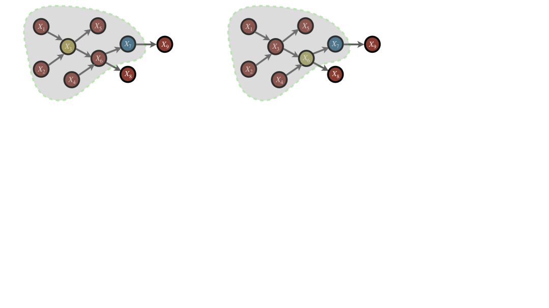
Figure 3: Example of the structure of a Bayesian network baseline model. The QoI is given by $f(X_{7})=X_{7}$ (blue color). We fix $X_{7}$ and we perturb one vertex at time, e.g. $X_{3}$ (left) and $X_{6}$ (right) in green color. The vertices involved in the graph can be classified into $l\in\bar{\rho}_{7}^{P}=\rho_{7}^{P}\cup\{7\}=\{1,2,3,4,5,6,7\}$ (vertices in the dashed area) and $\{8,9\}$ which are not in $\bar{\rho}_{7}^{P}$ (vertices outside of the dashed area), see left and right figures. Based on these figures and Lemma 3.1, the model sensitivity indices (29) over $\mathcal{D}^{\eta_{l}}_{l}$ and $\mathcal{D}^{\eta_{l}}_{l,P}$ is 0 for $l=8,9$, meaning that perturbations on vertices which are not ancestors of 7 do not affect the QoI, while perturbations on those vertices in $\bar{\rho}_{7}^{P}$ affect the QoI.



Notation. For the notation of this section, we refer to Section 2. Moreover, we denote $\bar{\rho}_{k}^{P}:=\rho_{k}^{P}\cup\{k\}$.


Let $f=f(X_{k})$ be a QoI depending only on vertex $k\in V$ and let $l\in V$ be another vertex. The first ambiguity set
$\mathcal{D}^{\eta_{l}}_{l}$
consists of all Bayesian networks (BN) $Q$ that differ from the baseline $P$ only in the CPD at the vertex $l$ while also allowing for the parents $\pi_{l}^{P}$ at $l$ to change. Namely,



(26)

$$\mathcal{D}^{\eta_{l}}_{l}=\left\{\begin{array}[]{cc}\textrm{all BN }Q:R(Q_{l|\pi_{l}^{Q}}\|P_{l|\pi_{l}^{P}})\leq\eta_{l}\textrm{ for all $x_{\pi_{i}^{P}}\cup x_{\pi_{i}^{Q}}$},\\
Q_{j|\pi_{j}}\equiv P_{j|\pi_{j}}\textrm{ for all }j\neq l\end{array}\right\}$$



where the parents $\pi_{l}^{Q}$ in model $Q$ may differ from the parents $\pi_{l}^{P}$ in model $P$.


The second ambiguity set $\mathcal{D}^{\eta_{l}}_{l,P}$ consists of all Bayesian networks (BN) $Q$ that differ from the baseline $P$ only in the CPD at the vertex $l$, however here we require that $\pi_{l}^{Q}=\pi_{l}^{P}=\pi_{l}$, i.e. parents are not allowed to change:



(27)

$$\mathcal{D}^{\eta_{l}}_{l,P}=\left\{\textrm{all BN }Q:R(Q_{l|\pi_{l}}\|P_{l|\pi_{l}})\leq\eta_{l}\textrm{ for all }x_{\pi_{l}},Q_{j|\pi_{j}}\equiv P_{j|\pi_{j}}\textrm{ for all }j\neq l\right\}$$



Note that



(28)

$$\mathcal{D}^{\eta_{l}}_{l,P}\subset\mathcal{D}^{\eta_{l}}_{l}.$$



We accordingly define the model sensitivity indices of the QoI $f(X_{k})$ as



(29)

$$I^{\pm}(f(X_{k}),P;\mathcal{Q}_{\eta_{l}})=\underset{Q\in\mathcal{Q}_{\eta_{l}}}{\mathrm{sup/inf}}\ \mathbb{E}_{Q}\left[f(X_{k})\right]-\mathbb{E}_{P}\left[f(X_{k})\right]$$



where $\mathcal{Q}_{\eta_{l}}=\mathcal{D}^{\eta_{l}}_{l}$ or $\mathcal{D}^{\eta_{l}}_{l,P}$ given by (26) and (27) respectively.


The evaluation of these model sensitivity indices will necessarily depend on the relative graph position of vertices $k,l\in V$ and in particular if $l$ is an ancestor of $k$. In particular we have the following:




Lemma 3.1.


Let $Q\in\mathcal{Q}_{\eta_{l}}$ where $\mathcal{Q}_{\eta_{l}}=\mathcal{D}^{\eta_{l}}_{l}$ or $\mathcal{D}^{\eta_{l}}_{l,P}$. Then



(30)

$$\;\;\;\;\;\mathbb{E}_{Q}\left[f(X_{k})\right]-\mathbb{E}_{P}\left[f(X_{k})\right]
=
\begin{cases}\mathbb{E}_{P_{\rho_{l}^{P}}}\left[\mathbb{E}_{Q_{l|\pi_{l}^{Q}}}\left[F\right]-{\mathbb{E}_{P_{l|\pi_{l}^{P}}}\left[F\right]}\right]&,l\in\bar{\rho}_{k}^{P}\\
0&,l\notin\bar{\rho}_{k}^{P}\end{cases}$$





where





$$F:=F(x_{l},x_{\rho_{l}^{P}})
=
\int_{\mathcal{X}_{\bar{\rho}_{k}^{P}\setminus\rho_{l}^{P}\cup\{l\}}}f(x_{k})\prod_{i\in\bar{\rho}_{k}^{P}\setminus\rho_{l}^{P}\cup\{l\}}P(dx_{i}|x_{\pi_{i}^{P}})$$







$$=
\mathbb{E}_{P_{\{k\}|\bar{\rho}_{l}^{P}}}\left[f(X_{k})\right]\,,$$





and the last expectation is with respect to the conditional distribution of $X_{k}$ given $X_{\bar{\rho}_{l}^{P}}=x_{\bar{\rho}_{l}^{P}}$.




The proof of Lemma 3.1 is a direct calculation of the difference between the expectations of $f(X_{k})$ and is based on a rearrangement between the CPDs of $X_{\rho_{k}^{P}\cup\{k\}}$, $X_{\rho_{l}^{P}}$ and $X_{l}$ with respect to $P$ and $Q$, see Appendix E, while a concrete computation of $F$ is given in Appendix 129 for the Bayesian network of Example C.


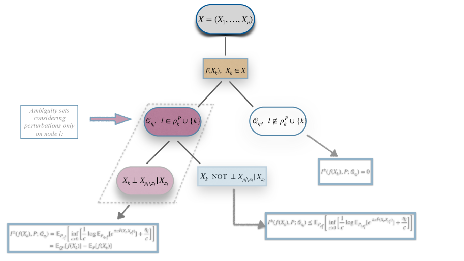
Figure 14: A schematic representation of how the set of vertices of a graph can be decomposed according to the relative position of vertex $k$ that corresponds to the QoI $f(X_{k})$, and a vertex $l$ such that perturbations of $P_{l|\pi_{l}}$ are considered. By Lemma 3.1, Theorem 3.2 and  3.4, the predictive uncertainty given by (29) with $l$ being in different parts of the decomposition varies: The set of vertices is first split as $X=(\bar{\rho}_{k}^{P})\cup(\bar{\rho}_{k}^{P})^{c}$. The predictive uncertainty $I^{\pm}(f(X_{k}),P;\mathcal{D}^{\eta_{l}}_{l})$ over models with only perturbed $P_{l|\pi_{l}}$ when $l\in\bar{\rho}_{k}^{P}$ is given by (3.2) and is tight in $\mathcal{D}^{\eta_{l}}_{l}$,while perturbation on $P_{l|\pi_{l}}$ when $l\notin\bar{\rho}_{k}^{P}$ do not affect the QoI and thus $I^{\pm}(f(X_{k}),P;\mathcal{Q}_{\eta_{l}})=0$. We then decompose the set of vertices $\bar{\rho}_{k}^{P}$ into $\{l:X_{k}\perp X_{\rho_{l}\setminus\pi_{l}}|X_{\pi_{l}}\}$ and its complement. The predictive uncertainty over $\mathcal{D}^{\eta_{l}}_{l,P}$ with $l$ in the former set is same as the one for $l\in\bar{\rho}_{k}^{P}$ with the difference that is tight on $\mathcal{D}^{\eta_{l}}_{l,P}$ contrary to the one in the latter set where the bound is not attained as well as is not tight.

Next, following the structure of Theorem 2.1 and using Lemma 3.1, we present our results on tightness and optimal distributions over $\mathcal{D}^{\eta_{l}}_{l}$ and $\mathcal{D}^{\eta_{l}}_{l,P}$ stated in Theorem 3.2 and  3.4 respectively. Theorem 3.4 could be thought of as a subcase of Theorem 3.2 due to (28), however tightness on $\mathcal{D}^{\eta_{l}}_{l,P}$ cannot be accomplished unless the additional condition (44) is assumed. All these results are summarized in a schematic in
Figure 14.



Theorem 3.2 (Model Sensitivity Indices–vary graph structure and CPD).


Let $P$ be a Bayesian network with density defined as (1), and $f(X_{k})$ be a QoI that only depends on $X_{k}$. Let also $\bar{f}(X_{k})$ be the centered QoI with finite moment generating function (MGF), $\mathbb{E}_{P}\left[e^{c\bar{f}(X_{k})}\right]$, in a neighborhood of the origin.


$(a)$ Tightness. For the model sensitivity indices defined in (29), there exist $0<\eta_{\pm}\leq\infty$, such that for any $\eta\leq\eta_{\pm}$,





$$\;\;\;\;\;\;\;I^{\pm}(f(X_{k}),P;\mathcal{D}^{\eta_{l}}_{l})
=
\underset{Q\in\mathcal{D}^{\eta_{l}}_{l}}{\mathrm{sup/inf}}\ \mathbb{E}_{Q}\left[f(X_{k})\right]-\mathbb{E}_{P}\left[f(X_{k})\right]$$







$$=
\begin{cases}\pm\mathbb{E}_{P_{\rho_{l}^{P}}}\left[\inf_{c>0}\Big{[}\frac{1}{c}\log\mathbb{E}_{P_{l|\pi_{l}^{P}}}\left[e^{\pm c\bar{F}}\right]+\frac{\eta_{l}}{c}\Big{]}\right]&,l\in\bar{\rho}_{k}^{P}\\
0&,l\notin\bar{\rho}_{k}^{P}\end{cases}$$






$$=
\mathbb{E}_{Q^{\pm}}\left[f(X_{k})\right]-\mathbb{E}_{P}\left[f(X_{k})\right]$$





where $\bar{F}$ is the centered function of $F$ defined in (3.1), $\eta_{l}\equiv\eta$
and $Q^{\pm}(\cdot)\equiv Q^{\pm}(\cdot\;;\pm c_{\pm})\in\mathcal{D}_{l}^{\eta_{l}}$ are Bayesian networks of the form (1) that depend on $\eta_{l}$ with $f(X_{k})$
and $c_{\pm}\equiv c_{\pm}(x_{\rho_{l}^{P}};\eta_{l})$ being functions of $x_{\rho_{l}^{P}}$, depend on $\eta_{l}$ and are determined by the equations



(33)

$$R(Q^{\pm}_{l|\pi_{l}^{Q^{\pm}}}\|P_{l|\pi_{l}^{P}})=\eta_{l}.$$



$(b)$ Graph Structure of $Q^{\pm}$. The optimal distributions $Q^{\pm}$ are the probability measures with densities given by



(34)

$$q^{\pm}(x_{i}|x_{\pi_{i}^{Q^{\pm}}})=\begin{cases}p(x_{i}|x_{\pi_{i}^{P}})&,i\neq l\\
\frac{e^{\pm c_{\pm}F(x_{l},x_{\rho_{l}^{P}})}}{\mathbb{E}_{P_{l|\pi_{l}^{P}}}\left[e^{\pm c_{\pm}F(X_{l},x_{\rho_{l}^{P}})}\right]}p(x_{l}|x_{\pi_{l}^{P}})&,i=l\end{cases}$$



The structure of the first and second part of (34) satisfy $\pi_{i}^{Q^{\pm}}\equiv\pi_{i}^{P}$ and $\pi_{l}^{P}\subset\pi_{l}^{Q^{\pm}}\subset\rho_{l}^{P}=\rho_{l}^{Q^{\pm}}$ respectively.





Proof 3.3.


The proof of $(a)$ and $(b)$ are worked together and is split into two main steps.


Step 1: Model sensitivity indices: For $l\in\bar{\rho}_{k}^{P}$, we denote $\pi_{l}:=\pi_{l}^{Q}\cup\pi_{l}^{P}$, and $\rho_{i}:=\rho_{i}^{Q}\cup\rho_{i}^{P}$ for all $i$. We define



(35)

$$Q(dx_{l}|x_{\pi_{l}}):=Q(dx_{l}|x_{\pi_{l}^{Q}})\textrm{ for all }x_{\pi_{l}},\qquad P(dx_{l}|x_{\pi_{l}}):=P(dx_{l}|x_{\pi_{l}^{P}})\textrm{ for all }x_{\pi_{l}}$$



We now use Lemma 3.1 and we further bound the right hand side of the first part of (3.2) as follows:







$$\;\;\;\;\;\underset{Q\in\mathcal{D}^{\eta_{l}}_{l}}{\mathrm{sup}}\ \mathbb{E}_{P_{\rho_{l}}}\left[\mathbb{E}_{Q_{l|\pi_{l}}}\left[F\right]-{\mathbb{E}_{P_{l|\pi_{l}}}\left[F\right]}\right]\leq\mathbb{E}_{P_{\rho_{l}}}\left[\underset{Q\in\mathcal{D}^{\eta_{l}}_{l}}{\mathrm{sup}}\ \mathbb{E}_{Q_{l|\pi_{l}}}\left[F\right]-{\mathbb{E}_{P_{l|\pi_{l}}}\left[F\right]}\right]$$






$$\qquad=\mathbb{E}_{P_{\rho_{l}}}\left[\underset{Q_{l}\in\mathcal{E}^{\eta_{l}}_{l}}{\mathrm{sup}}\ \mathbb{E}_{Q_{l|\pi_{l}}}\left[F\right]-{\mathbb{E}_{P_{l|\pi_{l}}}\left[F\right]}\right]$$




where $\mathcal{E}^{\eta_{l}}_{l}$ is the ambiguity set for CPDs at $l$ defined as



(37)

$$\mathcal{E}_{l}^{\eta_{l}}:=\{\textrm{all CPD }Q_{l|\pi_{l}}:R(Q_{l|\pi_{l}}\|P_{l|\pi_{l}})\leq\eta_{l}\textrm{ for all $x_{\pi_{l}}=x_{\pi_{l}}^{P}\cup x_{\pi_{l}}^{Q}$}\}$$



By using Lemma A.1, for any given $X_{\rho_{l}}=x_{\rho_{l}}$, we have



(38)

$$\underset{Q_{l}\in\mathcal{E}^{\eta_{l}}_{l}}{\mathrm{sup}}\ \mathbb{E}_{Q_{l|\pi_{l}}}\left[F\right]-{\mathbb{E}_{P_{l|\pi_{l}}}\left[F\right]}\leq\inf_{c>0}\Big{[}\frac{1}{c}\log\mathbb{E}_{P_{l|\pi_{l}}}\left[e^{c\bar{F}(X_{l},X_{\rho_{l}})}\right]+\frac{\eta_{l}}{c}\Big{]}.$$



Hence (3.3) implies that



(39)

$$\underset{Q\in\mathcal{D}^{\eta_{l}}_{l}}{\mathrm{sup}}\ \mathbb{E}_{Q}\left[f(X_{k})\right]-\mathbb{E}_{P}\left[f(X_{k})\right]\leq\mathbb{E}_{P_{\rho_{l}}}\left[\inf_{c>0}\Big{[}\frac{1}{c}\log\mathbb{E}_{P_{l|\pi_{l}}}\left[e^{c\bar{F}(X_{l},X_{\rho_{l}})}\right]+\frac{\eta_{l}}{c}\Big{]}\right]$$





Step 2: Tightness of the bounds:
As in Theorem 2.1, for any given $x_{\rho_{l}^{P}}$, we can consider the conditional measure $P^{c_{+}}_{l|\rho_{l}^{P}}$ defined by



(40)

$$\frac{dP^{c_{+}}_{l|\rho_{l}^{P}}}{dP_{l|\pi_{l}^{P}}}=\frac{e^{c_{+}(x_{\rho_{l}^{P}})F(x_{l},x_{\rho_{l}^{P}})}}{\mathbb{E}_{P_{l|\pi_{l}^{P}}}\left[e^{c_{+}(x_{\rho_{l}^{P}})F(X_{l},x_{\rho_{l}^{P}})}\right]}$$



where $c_{+}(x_{\rho_{l}^{P}})$ is a function of $x_{\rho_{l}^{P}}$ determined by $R(P^{c_{+}}_{l|\pi_{l}^{P}}\|P_{l|\pi_{l}^{P}})=\eta_{l}$.
By using Lemma A.2, we define



(41)

$$q^{+}_{l}(x_{l}|x_{\pi_{l}^{Q^{+}}}):=P^{c_{+}}_{l|\rho_{l}^{P}}\propto e^{c_{+}(x_{\rho_{l}^{P}})F(x_{l},x_{\rho_{l}^{P}})}p(x_{l}|x_{\pi_{l}^{P}})\quad\textrm{for all $x_{\pi_{l}^{Q^{+}}}$}\,.$$



Note that $\pi_{l}^{Q^{+}}$ depends on $\pi_{l}^{P}$ and $F(x_{l},x_{\rho_{l}^{P}})$, hence $\pi_{l}^{P}\subset\pi_{l}^{Q^{+}}\subset\rho_{l}^{P}$, and $\rho_{l}^{Q^{+}}=\rho_{l}^{P}$. Therefore, using the same notation as in Step 1, for $\pi_{l}=\pi_{l}^{Q^{+}}$, $\rho_{l}=\rho_{l}^{Q^{+}}$, we have



(42)

$$\mathbb{E}_{Q^{+}_{l|\pi_{l}}}\left[F\right]-{\mathbb{E}_{P_{l|\pi_{l}}}\left[F\right]}=\inf_{c>0}\Big{[}\frac{1}{c}\log\mathbb{E}_{P_{l|\pi_{l}}}\left[e^{c\bar{F}}\right]+\frac{\eta_{l}}{c}\Big{]}\ .$$



Furthermore, $R(Q^{+}_{l|\pi_{l}}\|P_{l|\pi_{l}})\leq\eta_{l}$ for all $x_{\pi_{l}}$ and hence $Q^{+}_{l}\in\mathcal{E}^{\eta_{l}}_{l}$. Let $q^{+}(x)=q^{+}_{l}(x_{l}|x_{\pi_{l}})\prod_{i\neq l}p(x_{i}|x_{\pi_{i}})$, then $Q^{+}\in\mathcal{D}^{\eta_{l}}_{l}$, and




$$\mathbb{E}_{Q^{+}}\left[f(X_{k})\right]-\mathbb{E}_{P}\left[f(X_{k})\right]=\mathbb{E}_{P_{\rho_{l}}}\left[\inf_{c>0}\Big{[}\frac{1}{c}\log\mathbb{E}_{P_{l|\pi_{l}}}\left[e^{c\bar{F}}\right]+\frac{\eta_{l}}{c}\Big{]}\right],$$



and thus (3.2) is proved. The calculations for $\underset{Q\in\mathcal{D}^{\eta_{l}}_{l}}{\mathrm{inf}}\ \mathbb{E}_{Q}\left[f(X_{k})\right]-\mathbb{E}_{P}\left[f(X_{k})\right]$ are similar.




We turn next to the ambiguity set $\mathcal{D}^{\eta_{l}}_{l,P}$ defined in (27) and its corresponding index.
Due to Theorem 3.2 and (28), the following uncertainty bound holds for $\mathcal{D}^{\eta_{l}}_{l,P}$:




(43)

$$I^{+}(f(X_{k}),P;\mathcal{D}^{\eta_{l}}_{l,P})
=
\underset{Q\in\mathcal{D}^{\eta_{l}}_{l,P}}{\mathrm{sup}}\ \mathbb{E}_{Q}\left[f(X_{k})\right]-\mathbb{E}_{P}\left[f(X_{k})\right]$$







$$\leq
\mathbb{E}_{P_{\rho_{l}}}\left[\inf_{c>0}\Big{[}\frac{1}{c}\log\mathbb{E}_{P_{l|\pi_{l}}}\left[e^{c\bar{F}(X_{l},X_{\rho_{l}})}\right]+\frac{\eta_{l}}{c}\Big{]}\right]$$





for any $l\in\bar{\rho}_{k}^{P}$, see also Figure 14. A similar bound holds for $I^{-}(f(X_{k}),P;\mathcal{D}^{\eta_{l}}_{l,P})$. However, the next theorem provides a condition on the Bayesian network $P$ that implies equality in (43), see (44) and Fig 4.



Theorem 3.4 (Model Sensitivity Indices–only vary CPD).


Let $P$ be a Bayesian network with density defined as (1), and $f(X_{k})$ be a QoI that only depends on $X_{k}$ with its centered QoI $\bar{f}(X_{k})$ having finite moment generating function (MGF), $\mathbb{E}_{P}\left[e^{c\bar{f}(X_{k})}\right]$, in a neighborhood of the origin.


$(a)$ For $l\notin\bar{\rho}_{k}^{P}$, $\mathbb{E}_{Q}\left[f(X_{k})\right]-\mathbb{E}_{P}\left[f(X_{k})\right]=0$, for any $Q\in\mathcal{D}^{\eta_{l}}_{l,P}$.


$(b)$ For $l\in\bar{\rho}_{k}^{P}$ satisfying the condition



(44)

$$X_{k}\perp X_{\rho_{l}\setminus\pi_{l}}|X_{\pi_{l}},$$



i.e., $X_{k}$ is independent of all the ancestors of $X_{l}$ given the parents of $X_{l}$, there exist probability measures $Q^{\pm}=Q^{\pm}(\eta)\in\mathcal{D}^{\eta_{l}}_{l,P}$ given by (33) - (34) such that



(45)

$$\mathbb{E}_{Q^{\pm}}\left[f(X_{k})\right]-\mathbb{E}_{P}\left[f(X_{k})\right]
=
\underset{Q\in\mathcal{D}^{\eta_{l}}_{l,P}}{\mathrm{sup/inf}}\ \mathbb{E}_{Q}\left[f(X_{k})\right]-\mathbb{E}_{P}\left[f(X_{k})\right]$$







For $l\in\bar{\rho}_{k}^{P}$ such that (44) is not satisfied, (43) holds.


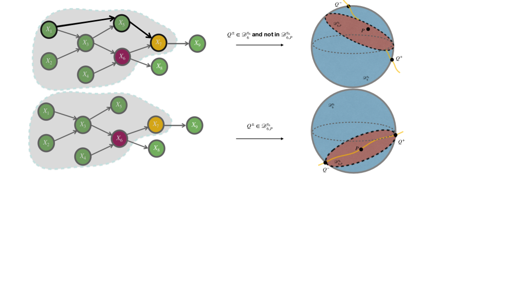
Figure 4: (Left) Two examples of the structure of a baseline Bayesian network. The QoI is $f(X_{7})$ in yellow (thus k=7) and $l=6$ in purple. (Right) Schematic of relationships between the ambiguity sets $\mathcal{D}^{\eta_{6}}_{6},\mathcal{D}^{\eta_{6}}_{6,P}$. They share the same boundary and thus we represent $\mathcal{D}^{\eta_{6}}_{6}$ as a sphere in blue, while $\mathcal{D}^{\eta_{6}}_{6,P}$ as an embedded disc in brown. The yellow curve in the both figures demonstrates the parametric family of Bayesian Networks $P^{c}$ with $dP^{c}_{l|\pi_{l}}=dP_{l|\pi_{l}}$ for $l\neq 6$ and $dP^{c}_{6|\pi_{6}}\propto\exp\{cF(x_{6},x_{\rho_{6}^{P}})\}dP_{6|\pi_{6}}$. The top graph does not satisfy condition (44) since $X_{1}$ is not conditionally independent of $X_{7}$ given $X_{\pi_{6}}$. This is illustrated through the path $X_{1}\to X_{5}\to X_{7}$ in black. The function $F$ given by (3.1) depends on $x_{1}$ and $x_{6}$ which makes the parents of $X_{6}$ in the optimizers $Q^{\pm}$ be different than its parents in $P$ and thus $Q^{\pm}\notin\mathcal{D}^{\eta_{6}}_{6,P}$ (in general) as illustrated in the top left picture. The bottom graph could achieve the equality in (3.2) since it satisfies condition (44) ($X_{\rho_{6}\setminus\pi_{6}}=\{X_{1},X_{2}\}$ are connected with $X_{7}$ only through $X_{3}\in X_{\pi_{6}}$). The function $F$ depends on $x_{3}$ and $x_{6}$ and $\pi_{6}^{Q}=\{3,4\}=\pi_{6}$ which makes $Q^{\pm}\in\mathcal{D}^{\eta_{6}}_{6,P}$, see bottom right picture. 







Proof 3.5.


Part $(a)$ and $(c)$ are straightforward consequences of Lemma 3.1 and (43) respectively. The proof of Part $(b)$ is as follows: For $l\in\bar{\rho}_{k}^{P}$ with $X_{k}\perp X_{\rho_{l}\setminus\pi_{l}}|X_{\pi_{l}}$, we have $F(x_{l},x_{\rho_{l}^{P}})=F(x_{l},x_{\pi_{l}})$,
then the proof is the same as the proof in Theorem 3.2. Indeed, let





(46)

$$q^{+}_{l}(x_{l}|x_{\pi_{l}^{Q^{+}}})=\frac{e^{\pm c_{+}F(x_{l},x_{\rho_{l}^{P}})}}{\mathbb{E}_{P_{l|\pi_{l}^{P}}}\left[e^{c_{\pm}F(X_{l},x_{\pi_{l}^{P}})}\right]}p(x_{l}|x_{\pi_{l}^{P}})\quad\textrm{for all $x_{\pi_{l}^{Q^{+}}}$ and $\pi_{l}^{Q^{+}}=\pi_{l}^{P}$},$$



where $c_{+}\equiv c_{+}(x_{\pi_{l}^{P}};\eta_{l})$ are functions of $x_{\pi_{l}}$ (since $F$ only depends on $x_{l}$ and $x_{\pi_{l}}$), depend on $\eta_{l}$ and are determined by the equations $R(Q^{+}_{l|\pi_{l}^{Q^{+}}}\|P_{l|\pi_{l}^{P}})=\eta_{l}$. Therefore, the density of $Q^{+}$ are given by $q^{+}(x)=q^{+}_{l}(x_{l}|x_{\pi_{l}^{Q^{+}}})\prod_{i\neq l}p(x_{i}|x_{\pi_{i}})$. Thus, $Q^{+}_{l}\in\mathcal{D}^{\eta_{l}}_{l,P}$ make (46) equality. Therefore we can conclude that



(47)

$$\underset{Q\in\mathcal{D}^{\eta_{l}}_{l,P}}{\mathrm{sup}}\ \mathbb{E}_{Q}\left[f(X_{k})\right]-\mathbb{E}_{P}\left[f(X_{k})\right]=\mathbb{E}_{P_{\rho_{l}}}\left[\inf_{c>0}\Big{[}\frac{1}{c}\log\mathbb{E}_{P_{l|\pi_{l}}}\left[e^{c\bar{F}(X_{l},X_{\rho_{l}})}\right]+\frac{\eta_{l}}{c}\Big{]}\right].$$



The case of $\underset{Q\in\mathcal{D}^{\eta_{l}}_{l}}{\mathrm{inf}}\ \mathbb{E}_{Q}\left[f(X_{k})\right]-\mathbb{E}_{P}\left[f(X_{k})\right]$ is treated similarly. By Lemma 3.1, for $l\notin\bar{\rho}_{k}^{P}$ and $Q\in\mathcal{D}^{\eta_{l}}_{l,P}$, $\mathbb{E}_{Q}\left[f(X_{k})\right]-\mathbb{E}_{P}\left[f(X_{k})\right]=0$.





Remark 3.6.


The condition $X_{k}\perp X_{\rho_{l}\setminus\pi_{l}}|X_{\pi_{l}}$ can be satisfied when $\rho_{l}\cap\rho_{i}\subset\pi_{l}$ for all $i\in\bar{\rho}_{k}\setminus\bar{\rho}_{l}$, i.e. any path from $X_{\rho_{l}\setminus\pi_{l}}$ to $X_{k}$ must go through $X_{\pi_{l}}$, for instance, all Markov chains, tree/polytree structure model, etc. Two simple examples where the assumption is satisfied or violated are shown in Figure 4. This condition is also satisfied by the baseline Bayesian network discussed in Section 7.





Remark 3.7.


Note that for the model sensitivity indices shown in (3.2) in Theorem 3.2 or the uncertainty bounds shown in (43) in Theorem 3.4, sometimes it might be practically difficult to find the infimum for every conditioning $\rho_{l}$. However, we can use an alternative looser bound by Jensen’s inequality, i.e.




(48)

$$I^{+}(f(X_{k}),P;\mathcal{D}^{\eta_{l}}_{l,P})
\leq
\mathbb{E}_{P_{\rho_{l}}}\left[\inf_{c>0}\Big{[}\frac{1}{c}\log\mathbb{E}_{P_{l|\pi_{l}}}\left[e^{c\bar{F}(X_{l},X_{\rho_{l}})}\right]+\frac{\eta_{l}}{c}\Big{]}\right]$$







$$\leq
\inf_{c>0}\Big{[}\mathbb{E}_{P_{\rho_{l}}}\left[\frac{1}{c}\log\mathbb{E}_{P_{l|\pi_{l}}}\left[e^{c\bar{F}(X_{l},X_{\rho_{l}})}\right]\right]+\frac{\eta_{l}}{c}\Big{]}$$





the model sensitivity index $I^{-}(f(X_{k}),P;\mathcal{D}^{\eta_{l}}_{l,P})$ can be treated analogously. Moreover, the corresponding bounds for $I^{\pm}(f(X_{k}),P;\mathcal{D}^{\eta_{l}}_{l})$ are similar. Moreover, if $\rho_{l}^{P}=\emptyset$, then expectation $\mathbb{E}_{P_{\rho_{l}^{P}}}\left[\cdot\right]$ does not enter in the overall calculations, and hence




$$I^{\pm}(f(X_{k}),P;\mathcal{D}^{\eta_{l}}_{l})=\inf_{c>0}\Big{[}\frac{1}{c}\log\mathbb{E}_{P_{l|\pi_{l}^{P}}}\left[e^{\pm c\bar{F}}\right]+\frac{\eta_{l}}{c}\Big{]},\qquad l\in\bar{\rho}_{k}^{P}$$



e.g for $l\in\{1,2,4\}$ and $k=7$ as illustrated in Figure 3. This is a special case, however it is used in the computation of the model sensitivity indices for the materials design problem in Section 7.





3.1 Gaussian Bayesian networks


Next, we develop model sensitivity indices $I^{\pm}(f(X_{k}),P;\mathcal{D}_{l}^{\eta_{l}})$, when $P$ is a Gaussian Bayesian Network satisfying (21), and $f(X_{k})$ depends on $X_{k}$ linearly. We first use Lemma 3.1, along with the fact that each model component is linear Gaussian of its parents, and compute $F$ and $\bar{F}$ explicitly. We show that $\bar{F}$ depends only on the $l$-th component and its parents $\pi_{l}^{P}$. Then, to implement Theorem 3.2, we calculate the MGF of $\bar{F}$ with respect to $P_{l|\pi_{l}^{P}}$. We prove that it no longer depends on $\pi_{l}^{P}$, due to cancellations between the terms involving $\pi_{l}^{P}$. Thus, the expectation $\mathbb{E}_{P_{\rho_{l}^{P}}}$ does not enter the overall computation of (3.2). Finally, we prove that $Q^{\pm}\in\mathcal{D}_{l,P}^{\eta_{l}}$, i.e. $Q^{\pm}$ are Gaussian Bayesian Networks with the same structure as $P$, without requiring condition (44) be satisfied, as explained in the proof of the theorem.



Theorem 3.8 (Model Sensitivity indices for Gaussian Bayesian Networks).


Let $P$ be a Gaussian Bayesian network satisfies (21), and $f(X_{k})=aX_{k}+b$ be a QoI only depends on $X_{k}$ linearly. Then,


 

For the model sensitivity indices defined in (29), we have



(49)

$$I^{\pm}(f(X_{k}),P;\mathcal{D}_{l}^{\eta_{l}})\equiv I^{\pm}(f(X_{k}),P;\mathcal{D}_{l,P}^{\eta_{l}})$$



and the optimizer $Q^{\pm}=Q^{\pm}(\eta)\in\mathcal{D}_{l,P}^{\eta_{l}}\subset\mathcal{D}_{l}^{\eta_{l}}$ given by (34) - (33) are also Gaussian Bayesian networks with same graph structure as $P$. Furthermore, for $l\in\pi_{k}^{P}$ and $l\notin\rho_{\pi_{j}}^{P}$ for all $j\in\pi_{k}$, $j\neq l$, we have



(50)

$$I^{\pm}(f(X_{k}),P;\mathcal{D}_{l}^{\eta_{l}})=\pm|\beta_{kl}|\sqrt{2a^{2}\sigma_{l}^{2}\eta_{l}}$$






 

Moreover, for any $l\in\rho_{k}^{P}$, we also have



(51)

$$I^{\pm}(f(X_{k}),P;\mathcal{D}_{l}^{\eta_{l}})=\pm|\tilde{\beta}_{kl}|\sqrt{2a^{2}\sigma_{l}^{2}\eta_{l}}$$



for a computable constant $\tilde{\beta}_{kl}$.








Proof 3.9.


Let $f(X_{k})=aX_{k}+b$ and $l\in\bar{\rho}_{k}$, then by a straightforward calculation of $F$ given by (3.1) can be expressed as



(52)

$$F(X_{l},X_{\rho_{l}})
=
 a\tilde{\beta}_{k_{0}}+a\sum_{j\in\rho_{l}}\tilde{\beta}_{kj}X_{j}+a\tilde{\beta}_{kl}X_{l}+b$$





for some computable $\tilde{\beta}_{k0},\tilde{\beta}_{kj}$ with $j\in\rho_{l}$ (see Example C where we compute $\beta_{kl}$ and $\tilde{\beta}_{kl}$). Furthermore, by using (21), the centered $F$ denoted by $\bar{F}$



(53)

$$\bar{F}(X_{l},X_{\pi_{l}})=\tilde{\beta}_{kl}a(X_{l}-\beta_{l0}-\beta_{l}^{T}X_{\pi_{l}})$$



and thus the MGF of $\bar{F}$ with respect to $P_{l|\pi_{l}}$ in the second equality of (3.2) is



(54)

$$\mathbb{E}_{P_{l|\pi_{l}}}\left[e^{\pm c\bar{F}(X_{l},X_{\pi_{l}})}\right]
=
\int_{\mathcal{X}_{l}}e^{\pm c_{\pm}\tilde{\beta}_{kl}ax_{l}}e^{\mp c_{\pm}\tilde{\beta}_{kl}a(\beta_{l0}+\beta_{l}^{T}x_{\pi_{l}})}dx_{l}$$








$$=
 e^{\pm c\tilde{\beta}_{kl}a(\beta_{l0}+\beta_{l}^{T}x_{\pi_{l}})+c^{2}\tilde{\beta}_{kl}^{2}a^{2}\frac{\sigma_{l}^{2}}{2}}e^{\mp c\tilde{\beta}_{kl}a(\beta_{l0}+\beta_{l}^{T}x_{\pi_{l}})}$$






$$=
 e^{c^{2}\tilde{\beta}_{kl}^{2}a^{2}\frac{\sigma_{l}^{2}}{2}}$$





We compute the minimization problem of (3.2) by following the steps given in the proof of Theorem 2.4.


Regarding the structure of $Q^{\pm}$, $Q^{\pm}\in\mathcal{D}^{\eta_{l}}_{l,P}$, i.e. the graph of $Q^{\pm}$ is same as $P$, as proved in Theorem 2.4 (see also Example C) where we showed that due to cancellations that may occur in the derivation of CPDs $q^{\pm}$ the graph remains the same.





4 Stress tests, Ranking and Correctability


Based on the model sensitivity indices discussed in Section 3 we build an iterative approach that ranks the Bayesian network components of the baseline $P$ according to their model sensitivity indices and subsequently improve its predictive ability for specific QoIs.
The model misspecification $\eta_{l}$ of the ambiguity sets can be either set up by the user e.g. when the data for component $l$ are very sparse or absent, or can be estimated from data, building a data-informed ambiguity set. Once $\eta_{l}$’s are specified, we rank the sensitivity indices $I^{\pm}(f(X_{k}),P;\mathcal{D}^{\eta_{l}}_{l})$ for all vertices $l$ based on their relative size.
Here the largest indices correspond to the most “sensitive” CPDs in the sense that they have the largest effect on the uncertainty of the QoI. From a Machine Learning perspective, such a ranking procedure is a form of interprability, i.e. the ability to identify cause and effect in a model [19, 52, 13] and explainability, i.e. the ability to explain model outputs based on modeling and data choices made during the learning of the baseline [1].


Once the ranking is completed, we turn to correcting the most influential components of a baseline Bayesian network, a task also referred to as correctability in Machine Learning; namely the ability to correct predictive
errors without introducing or (tightly) controlling any newly created errors (see Theorem 5.1 for Gaussian Bayesian Networks) [1, 38, 13]. To this end we need to assess the impact of limited data, seek additional data targeting specific model components,
or update some of the CPDs or the graph of the baseline Bayesian $\{G,P\}$. All these elements can be organized in a 4-step strategy discussed next, while they are implemented in an example in materials design for fuel cells in Section 7.


Notation. We remind that $P_{l|\pi_{l}}$ is the conditional distribution of $X_{l}$ with the given parents values $X_{\pi_{l}}=x_{\pi_{l}}$. However, we write $P_{l|X_{\pi_{l}^{P}}}$ when $X_{\pi_{l}}$ is still random variable and $P_{l|X_{\pi_{l}}=x_{\pi_{l}}}$ when we simply emphasize the dependence on given parents, see Step 1 below and the KL chain rule in Appendix F. Finally,
for each vertex $l\in V$ we use the notation $\pi_{l}:=\pi_{l}^{Q}\cup\pi_{l}^{P}$ when we consider simultaneously the parents for both models.


Step 1: Stress tests and model sensitivity. In this step, we determine the level of model misspecification $\eta_{l}$ for each component $l\in V$ of the baseline using data-informed or user-determined stress tests. In particular:


A. Data-informed stress tests.
For Bayesian networks (or parts thereof) for which there is a reasonable amount of data here
we construct data-informed ambiguity sets (5), (26) and (27) respectively. The corresponding levels of model misspecification $\eta,\eta_{l}$ are computed as distances between the baseline $P$ and the data distribution $Q$; the latter can be selected as a histogram or a Kernel Density Estimation (KDE).
In that sense, we provide surrogate values for the model misspecifications $\eta$ or $\eta_{l}$ taking into account the “real” model which is accessible only through the available data.
In these calculations we are
taking full advantage of the graph structure of the models.
First, we discuss the model uncertainty ambiguity set $\mathcal{D}^{\eta}$ in
(5). Using
the chain rule of KL divergence for Bayesian networks (Appendix F) we define a data-informed misspecification $\eta$ as



(56)

$$\eta:=R(Q\|P)=\sum_{l=1}^{n}\mathbb{E}_{Q}\left[\eta_{l}^{\pi_{l}}\right],\quad Q\in\mathcal{D}^{\eta}$$



where $\eta_{l}^{\pi_{l}}$ is a function of $X_{\pi_{l}}$ given by



(57)

$$\eta_{l}^{\pi_{l}}=\mathbb{E}_{Q}\left[R(Q_{l|X_{\pi_{l}^{Q}}}\|P_{l|X_{\pi_{l}^{P}}})\right]=\int_{\mathcal{X}_{l}}\log\frac{Q_{l|X_{\pi_{l}^{Q}}}}{P_{l|X_{\pi_{l}^{P}}}}Q_{l|X_{\pi_{l}^{Q}}}dx_{l}\,.$$



Second, for the case of model sensitivity, definition (56) reduces to



(58)

$$\eta_{l}=R(Q\|P)=\mathbb{E}_{Q}\left[\eta_{l}^{\pi_{l}}\right],\quad Q\in\mathcal{Q}_{\eta_{l}}$$



where $\mathcal{Q}_{\eta_{l}}$ is given by (26) or (27); to obtain this simplification of (56) we used the structure of the ambiguity sets $\mathcal{Q}_{\eta_{l}}$ where all CPDs are identical except for the one on the $l$-th vertex.


We now turn to the estimation of (56), (58).
We note that due to the graphical structure of Bayesian networks their estimation reduces to focusing on individual model components. Related recent ideas using subadditivity
for divergences or probability metrics of PGMs, instead of a full chain rule, were explored for statistical learning in [18]; such an approach could be also used here in an uncertainty quantification context.
Lastly, we can simplify the estimation of (56) or (58) by using an upper bound,
$\eta_{l}\leq\sup_{x_{\pi_{l}}}R(Q_{l|X_{\pi_{l}}=x_{\pi_{l}}}\|P_{l|X_{\pi_{l}}=x_{\pi_{l}}})\,.$
Under certain conditions we can also show that using KDE gives rise to consistent statistical estimator, see (140)-(143) for a Gaussian Bayesian network baseline.
Finally, we note that significant literature on statistical estimators
for divergences includes non-parametric
estimators [54], statistical estimators based on variational representations of divergences [56, 4], density-estimator based methods for estimating divergences in low-dimensions [45], estimators of divergence based on nearest-neighbor distances [71, 70, 60] and statistical estimators for Rényi Divergences [7].


B. User-determined stress tests.
Here we use $\eta_{l}\geq 0$ as a parameter to be tuned by hand to explore how different levels of uncertainty will affect the QoI;
for instance when we have very sparse or missing data and $\eta_{l}$’s are set by a user.
This is a form of non-parametric sensitivity analysis and is reminiscent in spirit of the stress tests used in finance and actuarial science, e.g. [11] to protect against sudden changes and extreme uncertainty under
various scenarios. In our Bayesian network context, individual model misspecification $\eta_{l}$, $l\in V$ for the model sensitivity indices $I^{\pm}(f(X_{k}),P;\mathcal{Q}_{\eta_{l}})$ can take arbitrary fixed values that correspond to model perturbations associated with local sensitivity analysis (small $\eta_{l}$) or global sensitivity analysis (larger $\eta_{l}$). Both local and global sensitivity analyses are conducted in the same mathematical
framework, therefore we have the flexibility to explore combinations of small/large model perturbations at different vertices of the Bayesian network.
From a practical point of view, these sensitivity computations can be done using only one fixed constructed Bayesian network (the baseline), yielding guarantees for entire neighborhoods of models.



Step 2: Ranking of model sensitivities. Once $\eta_{l}$’s are specified in Step 1 for each vertex $l$,
we calculate the model sensitivity indices $I^{\pm}(f(X_{k}),P;\mathcal{Q}_{\eta_{l}})$ using Theorem 3.2 and 3.4, where $\mathcal{Q}_{\eta_{l}}=\mathcal{D}^{\eta_{l}}_{l}$ or $\mathcal{D}^{\eta_{l}}_{l,P}$ are defined in (26) and (27). Subsequently we rank them according to their relative contributions



(59)

$$\frac{I^{+}(f(X_{k}),P;\mathcal{Q}_{\eta_{l}})}{\sum_{j}I^{+}(f(X_{k}),P;\mathcal{Q}_{\eta_{j}})}.$$



See also the example in Figure 9.


Step 3: Assessing the baseline. After we have ranked the model sensitivities in Step 2, we focus on the most impactful model components and assess their impact on the QoI $\mathbb{E}_{P}\left[f(X_{k})\right]$. Specifically, if the relative model uncertainty is less that an application-dependent tolerance $TOL$,



(60)

$$I^{+}(f(X_{k}),P;\mathcal{Q}_{\eta_{l}})\leq TOL\,,$$



then we decide to “trust” the model component $l$. If there are model components that do not satisfy (60), we proceed to the next step in order to correct the baseline model $P$. This is a form of interpretability, since we can systematically identify under-performing parts of the model. A related quantity that can also be used in (60) is the relative model sensitivity



(61)

$$\frac{I^{+}(f(X_{k}),P;\mathcal{Q}_{\eta_{l}})}{\mathbb{E}_{P}\left[f(X_{k})\right]}\,,$$



see for example
Figure 10.


Step 4: Model correctability. Once Steps 2 and 3 are completed, we turn to correcting the most influential components of the baseline Bayesian network $P$, a task also referred to as correctability in Machine Learning. We formulate mathematically this procedure in Section 5, however practically
we aim at reducing the index $I^{+}(f(X_{k}),P;\mathcal{D}^{\eta_{l}}_{l})$ for each vertex $l\in V$ that violates (60). This can be accomplished, for instance, by either acquiring additional data or updating the CPD of these specific vertices.
However, as we correct these targeted model components of the baseline, we also need to guarantee that we do not introduce new, bigger errors in the remaining components of the Bayesian network that would violate (60). Section 5 provides both theory and related practical implementation strategies to this end.



5 Mathematical analysis of correctability in Bayesian networks


In this section, we focus on the mathematical formulation of correctability in Bayesian Networks outlined in Step 4 of Section 4. Our methods are motivated by “correcting” a baseline model by either acquiring targeted high quality data, or updating the CPDs of the most under-performing components (see Step 3 of Section 4), or correcting the graph $G$ itself. We demonstrate these scenarios, their combinations and our mathematical methods on a materials screening problem for fuel cells in Section 7.


The intuition behind our correctability analysis lies in the model sensitivity results for the Gaussian case. By Theorem 3.8, the model sensitivity indices of a baseline $P$ for a targeted $l^{*}$-th CPD component are given by



(62)

$$I^{\pm}(f(X_{k}),P;\mathcal{D}_{l^{*},P}^{\eta_{l^{*}}})=\pm|\tilde{\beta}_{kl^{*}}|\sqrt{2\sigma_{l^{*}}^{2}\eta_{l^{*}}}\,.$$



Therefore, additional/better data or an improved CPD for the $l^{*}$-th vertex could allow us to build a new $l^{*}$-th CPD with a corresponding new Gaussian Bayesian model $\tilde{P}$ that is otherwise identical to $P$. Indeed, if we could guarantee a combination of




$$\tilde{\sigma}_{l^{*}}^{2}<\sigma_{l^{*}}^{2}\;\;\textrm{and/or}\;\;\tilde{\eta}_{l^{*}}<\eta_{l^{*}}$$



for the new model $\tilde{P}$ then we can quantify the improvement of the baseline $P$ using (62) and show that the indices of $\tilde{P}$ at $\l^{*}$ would decrease.


In general, we seek to correct the targeted $l^{*}$-th vertex of the baseline $P$ to obtain a new Bayesian network $\tilde{P}$
such that



(63)

$$I^{\pm}(f(X_{k}),\tilde{P};\mathcal{D}^{\eta_{l}}_{l})\leq I^{\pm}(f(X_{k}),P;\mathcal{D}^{\eta_{l}}_{l}),\qquad\textrm{all }\;l\neq l^{*}$$



and



(64)

$$I^{\pm}(f(X_{k}),\tilde{P};\mathcal{D}_{l^{*},P}^{\eta_{l^{*}}})<I^{\pm}(f(X_{k}),P;\mathcal{D}_{l^{*},P}^{\eta_{l^{*}}})\,.$$



In particular, (63) and (64) would imply that we can improve the CPD of the $l^{*}$ vertex and at the same time we do not decrease the performance of the rest of the Bayesian network.
The next theorem demonstrates that we can achieve (63) when $P$ is a Gaussian Bayesian network satisfying (21). Moreover, when $P$ is a general Bayesian network, we prove that new errors that may violate (63) can only be created in the descendant components of $l^{*}$, see also Remark 5.3.



Theorem 5.1.


(a) (Gaussian Bayesian Network) Consider $f(X_{k})=aX_{k}+b$ to be a QoI that only depends on $X_{k}$ linearly. Let also $P$ be a Gaussian Bayesian network satisfies (21). Suppose now that we construct a new Bayesian Network $\tilde{P}$ by only updating the CPD $p(x_{l^{*}}|x_{\pi_{l^{*}}})$ for some $l^{*}\in\rho_{k}$ as follows: we change the distribution of $\epsilon_{l^{*}}$ in (21) from Gaussian to another mean zero distribution denoted by $\tilde{p}(x_{l^{*}}|x_{\pi_{l^{*}}})$. Note that the graph structure of $\tilde{P}$ is the same as $P$. Then,



(65)

$$I^{\pm}(f(X_{k}),\tilde{P};\mathcal{D}^{\eta_{l}}_{l})=I^{\pm}(f(X_{k}),P;\mathcal{D}^{\eta_{l}}_{l}),\qquad\textrm{for all }\;l\neq l^{*}$$



where $I^{\pm}(f(X_{k}),P;\mathcal{D}^{\eta_{l}}_{l})$ is given by (50)-(51). Moreover, for the relative model sensitivity (61) the following holds:



(66)

$$\frac{I^{\pm}(f(X_{k}),\tilde{P};\mathcal{D}^{\eta_{l}}_{l})}{\mathbb{E}_{\tilde{P}}\left[f\right]}=\frac{I^{\pm}(f(X_{k}),P;\mathcal{D}^{\eta_{l}}_{l})}{{\mathbb{E}_{P}\left[f\right]}},\qquad\textrm{for all }\;l\neq l^{*}$$





(b) (Non Gaussian Bayesian Network) Let $f(X_{k})$ be a QoI that only depends on $X_{k}$. Let also $P$ be a non Gaussian Bayesian network. Let us suppose that we construct a new Bayesian Network $\tilde{P}$ with the same structure as $P$ by only updating the CPD $p(x_{l^{*}}|x_{\pi_{l^{*}}})$ for some $l^{*}\in\rho_{k}^{P}$. Then,



(67)

$$I^{\pm}(f(X_{k}),\tilde{P};\mathcal{D}^{\eta_{l}}_{l,P})=I^{\pm}(f(X_{k}),P;\mathcal{D}^{\eta_{l}}_{l,P}),\qquad\textrm{all }\;l\in\rho_{k}^{P}\textrm{ with }l<l^{*}$$



while the model sensitivity indices for any $l\in\rho_{k}^{P}$ with $l\geq l^{*}$ (descendant components) change and are given by Theorem 3.4.





Proof 5.2.


(a) First, updating $p(x_{l^{*}}|x_{\pi_{l^{*}}})$ with $l^{*}\in\rho_{k}$ does not affect the computation of $F$ defined in (3.1). This is straightforward by (3.1). In the case of a Gaussian Bayesian network, $F$ is given by (52). Second, if $l\neq l^{*}$, by (52), the MGF of $\bar{F}$ with respect to $\tilde{P}_{l|\pi_{l}}$ is always the same with the MGF computed with respect to $P_{l|\pi_{l}}$ (since $\tilde{P}_{l|\pi_{l}}=P_{l|\pi_{l}}$), see (54). However, it only changes when $l=l^{*}$. Moreover, the relative model sensitivity with respect to model $\tilde{P}$ satisfies (66), since $\tilde{P}_{l^{*}|\pi_{l^{*}}}:X_{l^{*}}=\beta_{l^{*}0}+\beta_{l^{*}}^{T}X_{\pi_{l^{*}}}+\tilde{\epsilon}_{l^{*}}$ with $\tilde{\epsilon}_{l^{*}}$ another mean zero distribution. Thus the expected values of $f(X_{k})$ with respect to $P$ and $\tilde{P}$ are equal.


(b) It is enough to observe that for any $l\in\rho_{k}^{P}$ with $l<l^{*}$, the MGF in Theorem 3.2 computed with the respect to $\tilde{P}_{l|\pi_{l}}^{P}=P_{l|\pi_{l}}^{P}$ and $P_{l|\pi_{l}}^{P}$ are equal and both depend on the ancestors of $\rho_{l}^{P}$, where $l^{*}\notin\rho_{l}^{P}$. Hence, (3.2) for both models is the same. Similarly, we prove the case $l\in\rho_{k}^{P}$ with $l\geq l^{*}$ (descendant components). Note that this time $l^{*}\in\rho_{l}^{P}$ and thus (3.2) is different for the two Bayesian Networks.




Both developed approaches are implemented in Section 7.3. For example, Theorem 5.1 (a) is applied when we update a CPD of the baseline Gaussian Bayesian Network by using a kernel-based (KDE) method,
see Figure 10. We refer to Section 7.3 for full details.



Remark 5.3.


Even if the conditions of Theorem 5.1 are not applicable, the ranking procedure of Step 2 & Step 3 in Section 4 can always identify the best candidates among the components of the graphical model for improvement relative to a QoI. Once we correct the component $l^{*}$ selected through ranking we need to recompute the relative model uncertainties in (60) for all vertices $l\in V$ and then determine the suitability of the corrected model. In fact, due to Theorem 5.1 (b) we only need to compute (60) for just the vertices $l$ in the descendants of $l^{*}$ since all the remaining ones are not affected by the model correction.





6 DFT-Informed Langmuir Model


In this section, we consider the Langmuir bimolecular adsorption model
that describes the chemical kinetics with competitive dissociative adsorption of hydrogen and oxygen on a catalyst surface [62, 24]. It is a multi-scale system of random differential equations with correlated dependencies in their parameters (kinetic coefficients), arising from quantum-scale computational data calculated using Density Functional Theory (DFT) (i.e quantum computations) for actual metals. The combination of chemical kinetics with parameter dependencies, correlations and DFT data gives rise naturally to a Bayesian network. However, the limited availability of the quantum-scale data creates significant model uncertainties both in the distributions of kinetic coefficients and their correlations, see for example Figure 5 (a).
Thus, we will quantify the ensuing model uncertainties by implementing our analysis in Section 2 and  3. Here, the equilibrium hydrogen and oxygen coverages are our QoIs and can be calculated by the dynamics of the chemical reaction network described by the following system of random ODEs with random (correlated) coefficients,



(68)

$$\frac{dC_{H^{*}}}{dt}
=k^{ads}_{H_{2}}P_{H_{2}}(1-C_{H^{*}}-C_{O^{*}})^{2}-k^{des}_{H_{2}}C^{2}_{H^{*}},\qquad C^{0}_{H^{*}}=C_{H^{*}}(0),$$




(69)

$$\frac{dC_{O^{*}}}{dt}
=k^{ads}_{O_{2}}P_{O_{2}}(1-C_{H^{*}}-C_{O^{*}})^{2}-k^{des}_{O_{2}}C^{2}_{O^{*}},\qquad C^{0}_{O^{*}}=C_{O^{*}}(0),$$




where $C_{H^{*}}$ and $C_{O^{*}}$ represent the hydrogen and oxygen coverages. $P_{H_{2}}$ and $P_{O_{2}}$ are the partial pressures of the gas phase species and are fixed.


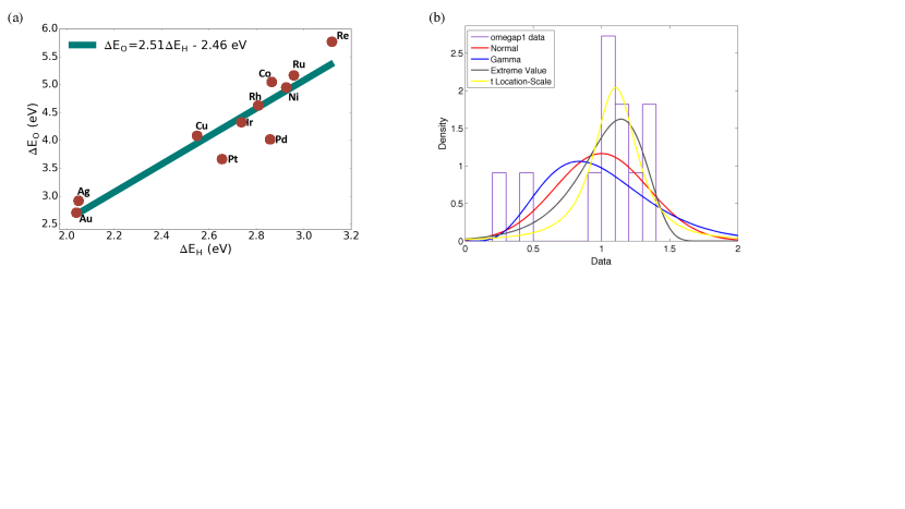
Figure 5: (a) Correlation between oxygen and hydrogen adsorption energies on metal surfaces as defined in (73), (b) Fit of $\omega$ in (73)
with various parametric distributions.


Then, the steady state solution of (68)-(69), which constitute our QoIs, is given by



(70)

$$\;\;\;\;\;\;\;\;\;\displaystyle{\hat{C}_{H^{*}}=\frac{(K_{H_{2}}P_{H_{2}})^{\frac{1}{2}}}{1+(K_{H_{2}}P_{H_{2}})^{\frac{1}{2}}+(K_{O_{2}}P_{O_{2}})^{\frac{1}{2}}},\quad\hat{C}_{O^{*}}=\frac{(K_{O_{2}}P_{O_{2}})^{\frac{1}{2}}}{1+(K_{H_{2}}P_{H_{2}})^{\frac{1}{2}}+(K_{O_{2}}P_{O_{2}})^{\frac{1}{2}}}}.$$



Here $K_{i}=\frac{k_{i}^{ads}}{k_{i}^{des}}$ for $i=H_{2},O_{2}$ and for each species they are related to electronic structure (DFT) calculations through an Arrhenius law [25]:



(71)

$$K_{H_{2}}
=e^{-\frac{G_{H_{2}}}{k_{B}T}}(P_{H_{2}}+P_{O_{2}})^{-1},\;\;G_{H_{2}}\propto-2\Delta E_{H}$$




(72)

$$K_{O_{2}}
=e^{-\frac{G_{O_{2}}}{k_{B}T}}(P_{H_{2}}+P_{O_{2}})^{-1},\;\;G_{O_{2}}\propto-2\Delta E_{O}$$




The constants $k_{B}$ and $T$ are the Boltzmann constant and the temperature respectively. In the above formulas, $G_{H_{2}}$ and $G_{O_{2}}$ are the hydrogen and oxygen Gibbs free energies of adsorption. Therefore, the coverages $\hat{C}_{H^{*}}$ and $\hat{C}_{O^{*}}$ are non-linear functions of $\Delta E_{H}$ and $\Delta E_{O}$. We refer to [24] for the chemistry background and analysis of the model. In [24], the authors have estimated the two binding energies for various metal catalyst surfaces via DFT calculations as illustrated in Figure 5(a). Furthermore, correlations between
$\Delta E_{O}$ and $\Delta E_{H}$ are captured by a statistical linear model



(73)

$$\Delta E_{O}=a\Delta E_{H}+b+\omega$$



where $\omega$ is a random variable. The distribution of $\omega$ can be determined by fitting the residual data from linear regression using Maximum Likelihood Estimation (MLE), Figure 5(b).


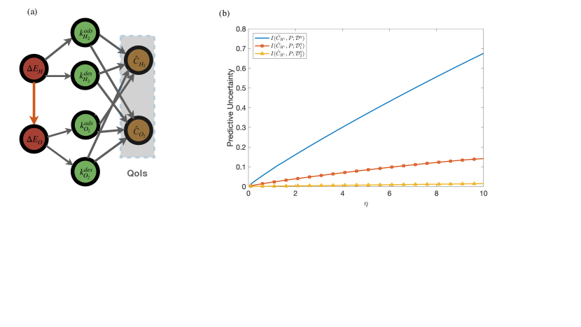
Figure 6: (a) Graph structure of the baseline Bayesian network $P$ in (76) built by data (74) and (75),
physics knowledge (71), (72), (75) and the steady state of the ODEs given by (70).
(b) We consider the QoIs (70) of (76): the blue line represents the model uncertainty index $I^{\pm}(f,P;\mathcal{D}^{\eta})$ as a function of $\eta$ (Theorem 2.1);
the red and yellow lines are respectively the model sensitivity indices $I^{\pm}(f,P;\mathcal{D}^{\eta}_{1})$ and $I^{\pm}(f,P;\mathcal{D}^{\eta}_{2})$ (Theorem 3.2) for $p(\Delta E_{H})$ and $p(\Delta E_{O}|\Delta E_{H})$ where $\mathcal{D}^{\eta}_{1}$ indicates the perturbation on $p(\Delta E_{H})$ and $\mathcal{D}^{\eta}_{2}$ for $p(\Delta E_{O}|\Delta E_{H})$.



In (73) we select a Gaussian distribution for $\omega$ (red line in Figure 5 (b)) as the baseline CPD for the correlation in Figure 5:



(74)

$$p(\Delta E_{O}|\Delta E_{H})=\mathcal{N}(a\,\Delta E_{H}+b,\sigma_{\omega}^{2}).$$



Next we model the distribution of the prior $p(\Delta E_{H})$. Based on physical constraints (e.g. positivity of the random variable without physical upper bound), in [24] the distribution of $\Delta E_{H}$ was selected to be a gamma distribution with mean $x_{H}$ with standard deviation given by the difference between experiment and DFT, $(x_{H}-y_{H})$,



(75)

$$p(\Delta E_{H})=\frac{1}{b_{H}^{a_{H}}\Gamma(a_{H})}\Delta E_{H}^{\ a_{H}-1}\exp\left(-\frac{\Delta E_{H}}{b_{H}}\right)\quad\mbox{for}\quad\Delta E_{H}>0,$$



where $a_{H}=x_{H}^{2}/(x_{H}-y_{H})^{2}$ and $b_{H}=(x_{H}-y_{H})^{2}/x_{H}$. This is a case with very little data $(x_{H},y_{H})$ and only some reasonable physical constraints without any further knowledge on the model, therefore model uncertainty in (75) is evident.


We now build the baseline Bayesian network $P$ by combining the following ingredients:
data through (74) and (75),
physics and expert knowledge in (71), (72), (75) and the steady state of the ODEs (QoI) given by (70), see also Figure 6. We obtain the following Bayesian network and the corresponding CPDs:



(76)

$$p(x)=\underbrace{p(\hat{C}_{H^{\ast}},\hat{C}_{O^{\ast}}|K_{H_{2}},K_{O_{2}})}_{\eqref{eq:Langmuir equilibrium}}\prod_{i=H_{2},O_{2}}\!\!\underbrace{p(K_{i}|\Delta E_{i})}_{\eqref{eq:Arrhenius1},\eqref{eq:Arrhenius2}}\underbrace{p(\Delta E_{O}|\Delta E_{H})}_{\eqref{eq:langmuir PGM_p2}}\underbrace{p(\Delta E_{H})}_{\eqref{eq:langmuir PGM_p1}}$$



In the above formula, $p(\hat{C}_{H^{\ast}},\hat{C}_{O^{\ast}}|K_{H_{2}},K_{O_{2}})$ and $p(K_{i}|\Delta E_{i})$ are deterministic, while the only random parts in $P$ are $p(\Delta E_{O}|\Delta E_{H})$ and $p(\Delta E_{H})$.


In the process of building the baseline model $P$ above, the sparse data in Figure 5 for (74) and the lack of both knowledge and (almost any) data in (75)
create model uncertainties for the prediction of the QoIs in (70). We quantify these uncertainties by implementing the model uncertainty index of Theorem 2.1 and the model sensitivity indices of Theorem 3.2; see Figure 6 (b) where we readily see how the indices change for different values $\eta$; the implementation of the indices was carried out through Monte Carlo simulation of the moment generating functions.
Moreover, we observe that for the QoIs (70) the impact of uncertainties in the prior $p(\Delta E_{H})$ are significantly higher than in the correlation $p(\Delta E_{O}|\Delta E_{H})$ when we perturb with same model misspecification $\eta$.
Finally, we note that due to the lack of data in (75), we elected to perform the user-determined stress tests of Step 1.B of Section 4 where the user selects various levels of model misspecification $\eta$.



7 Model Uncertainty for Sabatier’s Principle


We study Bayesian networks built for trustworthy prediction of materials screening to increase the efficiency of chemical reactions in catalysis. Our starting point is Sabatier’s principle which describes the efficiency of a catalyst [62] through the so-called “volcano curve”, e.g. the black curve in Figure 7(c). The volcano curve suggests that high catalytic activity is exhibited when the binding interaction between reactants and catalysts is neither too strong nor too weak, i.e. at the peak of the volcano marked by a star in Figure 7(c). For this reason Sabatier’s principle is widely viewed as an important criterion for screening materials for increased efficiency in catalysis. Our ultimate goal here is to understand how various uncertainties can affect the shape and position of the volcano curve and its peak.


Here we consider the Oxygen Reduction Reaction (ORR) which is a known performance bottleneck in fuel cells [63].
The ORR reaction depends on the formation of surface hydroperoxyl ($OOH^{\ast}$) from molecular oxygen ($O_{2}$), and water ($H_{2}O$) from surface hydroxide ($OH^{\ast}$) [67]. The complete mechanism [14, 2, 43] involves four electron exchange steps with reactions (R1) and (R4) being slow, see Figure 7(a). Therefore, the discovery of new materials will have to rely on speeding up the two slowest reactions in order to accelerate the entire ORR mechanism.
Furthermore, such a physicochemical system has hidden correlations between variables which have emerged after statistical analysis of data [26]. In particular, the corresponding Gibbs energies of reactions (1) and (4) denoted by $-\Delta G_{4}\equiv y_{1}$ and $-\Delta G_{1}\equiv y_{2}$ are computed as linear combinations of free energies of species and are regressed versus the oxygen binding energy $\Delta G_{O}\equiv x$ calculated by DFT calculations. The oxygen binding energy $x$ is chosen as a descriptor in [26] since it is the natural coordinate arising from Sabatier’s principle. The principle is graphically represented by the volcano curve , i.e. the solids black lines in Figure 7(c) which is a function of the descriptor.
Therefore, the QoI considered here is the optimal oxygen binding energy $\Delta G_{O}$ denoted by $x_{O^{*}}^{P}$ and identified as the maximum of the volcano curve:



(77)

$$x_{O^{*}}^{P}:=\mathrm{argmax}_{x_{0}}\left[\min\{\mathbb{E}_{P}\left[y_{1}|x_{0}\right],\mathbb{E}_{P}\left[y_{2}|x_{0}\right]\}\right]\,.$$



Starting from this QoI we build a Bayesian network in Figure 7(b)that includes expert knowledge (volcano curves), as well as various available experimental and computational data and their correlations or conditional independence.


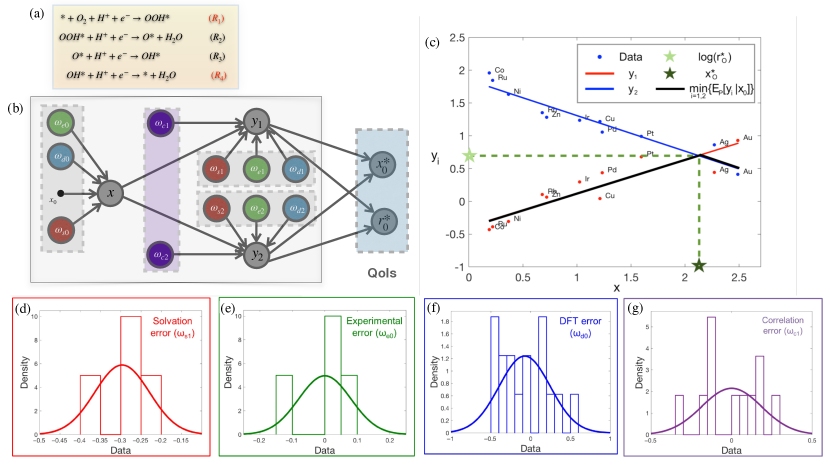
Figure 7: (a) ORR reaction steps (R1 to R4) in hydrogen
fuel cells, (b) Bayesian network for ORR. The construction of the Bayesian network (Section 7.1) is based on expert knowledge, physicochemical modeling and statistical analysis of data. We include these random variables into the Bayesian network and build the directional relationships (connection/arrows)
between corresponding random variable $x$ or $y_{i}$. We build a Gaussian Bayesian network, i.e., all CPDs are Gaussians which are fitted to available data using MLE (see histogram approximations in (d-g)). Note the conditional independence between the $y$-variables, assumed based on expert knowledge. (c) The QoI of the ORR model is the optimal oxygen binding energy $x_{O^{\ast}}^{P}$ and is identified when the two reaction energies are equal by physical modeling (marked with a star). (d-f) Here we model different kinds of errors in $x$ and $y_{i}$, given expert knowledge.



7.1 Construction of the ORR Bayesian network for the QoI (77)


First, we relate the QoI with the $y_{i}$’s and then we include errors from different sources in $x$ and $y_{i}$’s.
More precisely,


(1) [Graph] We first build the directed graph for the Bayesian network. The first selected vertices in the graph are the QoIs $x_{O^{\ast}}^{P}$, $r_{O^{\ast}}^{P}$, as well as $y_{i}$’s and $x$, see gray vertices in Fig. 7 (b). Subsequently,


 

Through the statistical independence test [73], we learn that $y_{1}$ and $y_{2}$ depend on $x$ and are conditionally independent given $x$ as illustrated in Figure 7 (b).



 

The construction of $x$ comes from the DFT data (using quantum calculations) for the oxygen binding energy given the real unknown value $x_{0}$. As mentioned in the beginning of the section, $x$ is also selected to be the descriptor by expert knowledge (see also the supplementary material of [26]) and justifies the conditional relationships between $x$ and $y_{i}$’s.



 

The evaluations of the QoIs depend on the values of $y_{i}$’s for each $x_{0}$ due to the volcano curve of the Sabatier’s principle.



Overall, in (1) we built part of the network structure for $x$, $y_{1}$, $y_{2}$ and the QoI using a constraint-based method [66], which selects a desired structure based on constraints of dependency among variables.


(2)[CPD] Next, we build the individual CPDs on the graph constructed above.


 

We include statistical correlations between DFT (quantum calculation) data for $x$ and $y_{i}$, see data in [26]. We model the residual using a linear model with a random correlation error denoted by $\omega_{ci}$, see (79).



 

We model as random variables and incorporate in the Bayesian network different kinds of errors in $x$ and $y_{i}$’s
from the following sources: $\omega_{ei}$ is the error in experimental data, $\omega_{di}$ is error between quantum and experimental values and $\omega_{si}$ is error due to solvation effects; all are calculated by DFT, see the corresponding data in [26]. See (79).



More specifically, after conducting independence tests on the corresponding data, and also based on expert knowledge or intuition [26] we assume that the random variables $\omega$ are independent. Based on the graph construction above we obtain the Bayesian network



(78)

$$p(\mathbf{x}|x_{0})=\prod_{i=1,2}p(y_{i}|x,\omega_{ei},\omega_{di},\omega_{si},\omega_{ci})\cdot p(x|\omega_{e0},\omega_{d0},\omega_{s0},x_{0})\cdot\!\!\!\!\!\!\!\!\!\prod_{\begin{subarray}{c}j=e_{k},d_{k},s_{k},c_{1},c_{2}\\
k=0,1,2\end{subarray}}\!\!\!\!\!\!\!\!\!\!p(\omega_{j})$$



where $\mathbf{x}=(x,y_{1},y_{2},\omega_{e0},\omega_{d0},\omega_{s0},\omega_{e1},\omega_{d1},\omega_{s1},\omega_{c1},\omega_{e2},\omega_{d2},\omega_{s2},\omega_{c2})$.
The baseline CPDs in (78) are constructed as linear Gaussian models, namely for $i=1,2$:



(79)

$$y_{i}=\beta_{y_{i},0}+\beta_{y_{i},x}x+\omega_{ei}+\omega_{di}+\omega_{si}+\omega_{ci}\quad\textrm{and}\quad x=x_{0}+\omega_{e0}+\omega_{d0}+\omega_{s0}\,.$$



The CPDs for each vertex are selected as



(80)

$$p(y_{i}|x,\omega_{ei},\omega_{di},\omega_{si},\omega_{ci})
=\mathcal{N}(\beta_{y_{i},0}+\beta_{y_{i},x}x+\omega_{ei}+\omega_{di}+\omega_{si}+\omega_{ci},0)$$




(81)

$$p(x|\omega_{e0},\omega_{d0},\omega_{s0},x_{0})
=\mathcal{N}(x_{0}+\omega_{e0}+\omega_{d0}+\omega_{s0},0)$$




(82)

$$p(\omega_{j})
=\mathcal{N}(\beta_{j,0},\sigma_{j}^{2})$$




where $i=1,2$, and $j=e0,d0,s0,e1,d1,s1,c1,e2,d2,s2,c2$. Then the resulting baseline model
(78) is a Gaussian Bayesian network.
Subsequently we use the global likelihood decomposition method [48] to learn the parameters $\beta_{y_{i},0},\beta_{y_{i},x}$ and $\sigma_{j}$. The outcomes are given in Table 1. This approach is essentially a Maximum Likelihood Estimation (MLE) on PGMs (see [48, Chapter 17.2]), that exploits a fundamental scalability property that allows us to “divide and conquer” the parameter inference problem on the graph. We can also employ a Bayesian approach instead of MLE, see for instance [48] for the case of PGMs.




7.2 Model sensitivity, stress tests and ranking


Here, we implement the four-step strategy of Section 4 to the ORR model by using data-informed stress tests or user-determined stress tests (Step 1.A and Step 1.B of Section 4). The primary goal is to quantify and rank the impact of model uncertainties
from each component of the Bayesian network through the model sensitivity
indices in Section 3. Next, we compute these model sensitivity indices for the QoI $x_{O^{*}}^{P}$ in (77), namely



(83)

$$\underset{Q\in\mathcal{D}^{\eta_{l}}_{l,P}}{\mathrm{sup/inf}}\left\{x_{O^{*}}^{Q}-x_{O^{*}}^{P}\right\}$$



for $l\in\{ei,di,si,ci,e0,d0,s0\}$ with $i=1,2$. To this end, we first
use Theorem 3.8 for $i=1,2$ to obtain



(84)

$$I^{\pm}(y_{i},P;\mathcal{D}^{\eta_{l}}_{l,P})=\pm|\tilde{\beta}_{y_{i},\omega_{l}}|\sqrt{2\sigma_{l}^{2}\eta_{l}}\ ,$$



with $\sigma_{l}$ and $\tilde{\beta}_{y_{i},\omega_{l}}$ given in (80) and Table 2 respectively. Subsequently we
solve the optimization problem for $x_{O}=x_{O^{\ast}}^{P}$ and obtain the bounds for $x_{O^{*}}^{Q}-x_{O^{*}}^{P}$ as shown in Figure 8 and given by



(85)

$$\frac{-\sqrt{2\sigma_{l}^{2}\eta_{l}}}{\beta_{y_{1},x}-\beta_{y_{2},x}}\leq x_{O^{*}}^{Q}-x_{O^{*}}^{P}\leq\frac{\sqrt{2\sigma_{l}^{2}\eta_{l}}}{\beta_{y_{1},x}-\beta_{y_{2},x}}$$



for $l=ei,di,si,ci$ and $i=1,2$; note that the model uncertainty of $\omega_{l}$ only affects $y_{i}$ according to the ORR Bayesian network. Furthermore,



(86)

$$\frac{-(|\beta_{y_{1},x}|+|\beta_{y_{2},x}|)\sqrt{2\sigma_{l}^{2}\eta_{l}}}{\beta_{y_{1},x}-\beta_{y_{2},x}}\leq x_{O^{*}}^{Q}-x_{O^{*}}^{P}\leq\frac{(|\beta_{y_{1},x}|+|\beta_{y_{2},x}|)\sqrt{2\sigma_{l}^{2}\eta_{l}}}{\beta_{y_{1},x}-\beta_{y_{2},x}}$$



for $l=e0,d0,s0$ as the model uncertainty of $\omega_{l}$ affects both $y_{1}$ and $y_{2}$. Here $\beta_{y_{i},x}$ are the coefficients given by the first CPD in (80). The complete algebraic calculation of (85) and (86) is given in the Appendix I.1.


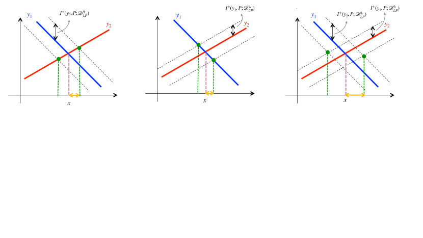
Figure 8: Typical model uncertainty bounds $I^{\pm}(y_{i},P;\mathcal{D}^{\eta_{l}}_{l,P})\,,i=1,2$ computed by (84). The model uncertainty for the QoI $x_{O^{\ast}}^{P}$ (see Figure 7(c)) is computed by (85)-(86) and demonstrated in yellow for model misspecification $\eta_{l}$ in $P(\omega_{l})$: (a) for $l=e1,d1,s1,c1$, $I^{\pm}(y_{1},P;\mathcal{D}^{\eta_{l}}_{l,P})=\pm\sqrt{2\sigma_{l}^{2}\eta_{l}}$; (b) for $l=e2,d2,s2,c2$, $I^{\pm}(y_{2},P;\mathcal{D}^{\eta_{l}}_{l,P})=\pm\sqrt{2\sigma_{l}^{2}\eta_{l}}$; (c) for $l=e0,d0,s0$, $I^{\pm}(y_{i},P;\mathcal{D}^{\eta_{l}}_{l,P})=\pm|\beta_{y_{i},x}|\sqrt{2\sigma_{l}^{2}\eta_{l}}$, $i=1,2$.



Then by implementing Step 2 of Section 4, we rank the model components as demonstrated in Figure 9. There we plot (59) as a pie chart, where the most impactful components are depicted.






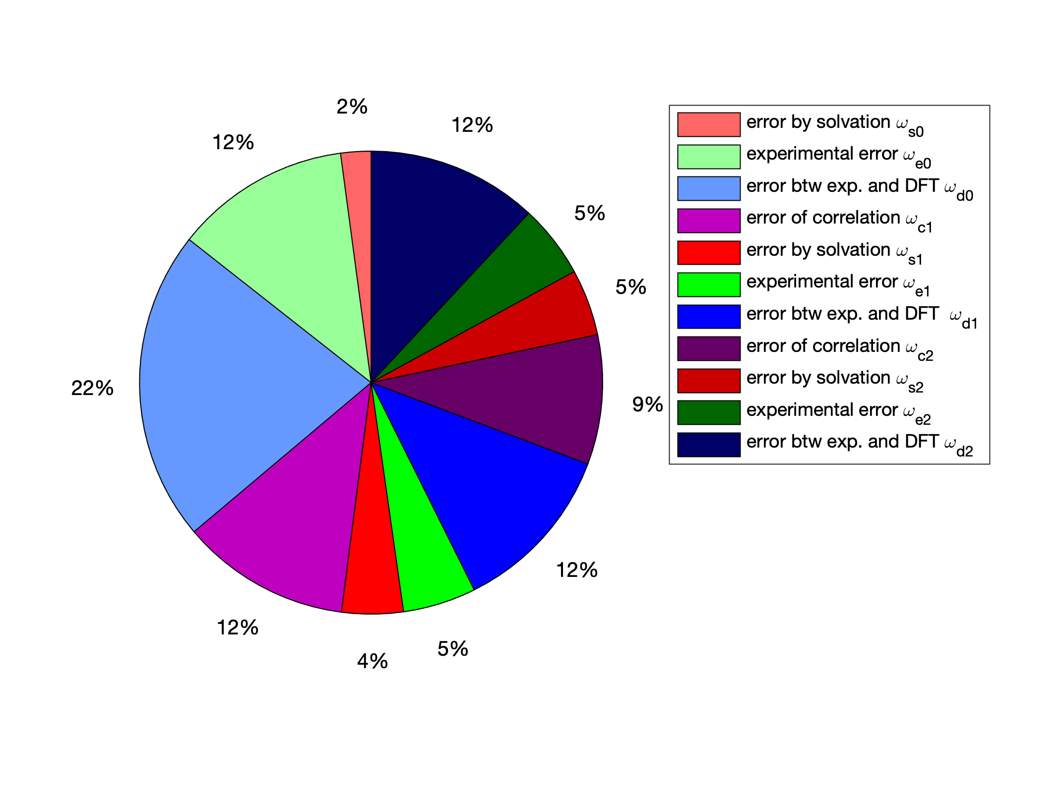
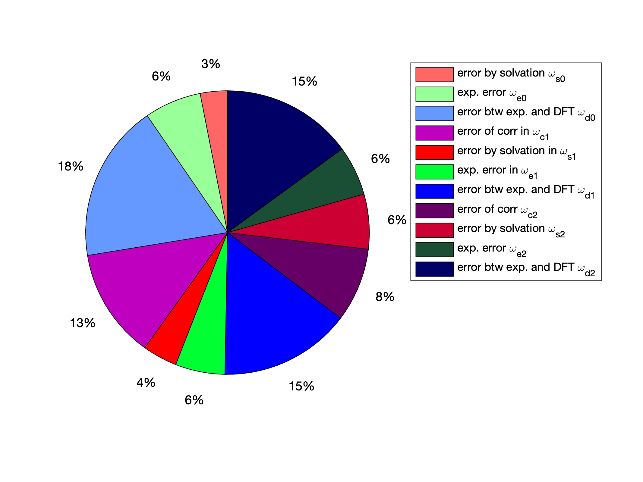
Figure 9: Relative model sensitivities (59) for the QoI $x_{O^{\ast}}^{P}$
in each ORR Bayesian network mechanism in Figure 7 (b). (Left) User-determined stress test (Step 1.B. in Section 4); $\eta_{l}$ has a fixed value for all $l$; the particular value does not matter since it is canceled out by the ratio in (59). (Right)
Data-informed stress test (Step 1.A. in Section 4);
$\eta_{l}=R(data\|P_{l})$ selected as a distance of each CPD from the available data.




Remark 7.1 (Propagation/Non-Propagation of
Uncertainties to the QoIs).


The discrepancies in the propagation of model misspecification to the QoI between different Bayesian network components is depicted in Figure 9. In particular, in Figure 9 (Left) the same user-selected model misspecification $\eta_{l}$ is applied on all ORR Bayesian network vertices. However not all propagate and affect the same the QoI. See also the example in
Figure 15.





Remark 7.2.


The construction of the ORR Bayesian network and its model uncertainty was carried out in [26] for the optimal oxygen binding energy defined differently than (77), that is as $\mathrm{argmax}_{x_{0}}\mathbb{E}_{P}\left[y|x_{0}\right]$ with $y|x_{0}=\min\{y_{1}|x_{0},y_{2}|x_{0}\}$. This is an alternative mathematical description of the same concept, however (77) allows to explicitly calculate the model sensitivity indices given by (84)-(86) and provide clear insights in what model elements and uncertainties affect them the most. On the other hand, in [26] the model sensitivity indices provided by Theorem 3.2 can only be calculated computationally.






7.3 Correctability of the ORR Bayesian Network


Here we use the earlier model uncertainty/sensitivity analysis to first identify and then correct the most impactful components in several ways as discussed in Step 4 of Section 4 and in the theoretical results on correctability in Section 5.


1. Including targeted high quality data. We seek data that lead to the reduction of the variance $\sigma_{l^{\ast}}^{2}$ for some $l^{\ast}\in L$ (see Step 3 of Section 4), while the model misspecification $\eta_{l^{\ast}}$ does not increase or the increment is much smaller than the reduction of $\sigma_{l^{\ast}}^{2}$. Notice that in this case the model remains a Gaussian Bayesian network. For the ORR Bayesian network, it turns out that we can add more data using DFT calculations for bimetallics to reduce the relative error for the correlation errors $\omega_{ci}$, $\sigma_{ci}^{2}$; see the bimetallics data set in [26]. Then the model sensitivity indices of $y_{i}$ on $\omega_{ci}$, $I^{\pm}(y_{i},P;\mathcal{D}^{\eta_{l}}_{l,P}),\,l=\omega_{ci}$ given by (84) and the model misspecification $\eta_{\omega_{ci}}$ are reduced. Consequently, the model sensitivity indices of $x_{O^{\ast}}^{P}$ does so as well, see (85). The relative predictive uncertainty (61) of such an updated model is demonstrated in Figure 10 (Center),
updated model 2.


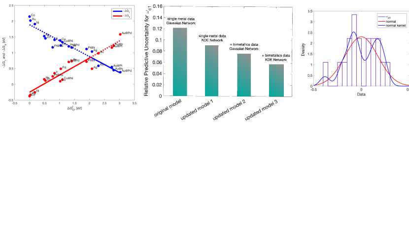
Figure 10: (Left) DFT-computed data for reaction energies with respect to different metals/oxygen binding energies. Here bimetallics data are also included in addition to the single metals in Figure 7 (c). (Center) Different relative model sensitivities (61)
when we: only perturb the model of $\omega_{c1}$ by $\eta_{c1}=R(data\|P_{c1})$ when $P_{c1}$ is Gaussian with the original single-metal data; or using a KDE given by (142) with the original data (updated model 1); or using a Gaussian with the additional bimetallics data (updated model 2); or using both KDE and Bimetallics data (updated model 3). (Right) Baseline model (Gaussian) of $\omega_{c1}$ (red curve) and the updated model (normal-kernel density estimation, blue curve) and additional bimetallics data in this figure (Left).


2. Increasing the complexity of CPDs. We reduce the model misspecification $\eta_{l^{\ast}}$ by picking a better model $\tilde{P}_{l^{\ast}}$ than the baseline model $P_{l^{\ast}}$ for the $l^{*}$ component. The new model should represent the (fixed) available data more accurately by using a kernel-based method. In this case the new model is a mixture of Gaussian and kernel-based networks [48].
For example, we replace the linear, Gaussian model for $\omega_{c1}$ demonstrated in Fig. 7 (g) with a linear, kernel-based model as shown in Figure 10 (Right). Then we can reduce the model sensitivity indices by decreasing the model misspecification $\eta_{l^{*}}$ without introducing new errors in the remaining components of the Bayesian Network as proved in Theorem 5.1 (a).


Moreover,
we can combine the approaches above to reduce the model sensitivity indices. For example, after adding more bimetallics data, we first reduce the model sensitivity indices for the correlation errors $\omega_{ci}$. Then we further reduce the indices of $\omega_{c1}$ by replacing the corresponding component of the baseline model for $\omega_{c1}$ (Gaussian model) by normal kernel density estimator without increasing the indices of the remaining nodes (see Theorem 5.1 (a)). The new model is the updated model 3 in Figure 10 (Center).
We can compute the model sensitivity indices for the updated mixed model, where $P_{l}$ could be KDE or another distribution, using
Theorem 3.4 and in particular (43).


3. Increasing the complexity of the graph. Here, we discuss how model sensitivity indices can investigate the change in graph structure. The available data for solvation energies in Figure 11 (Left), indicate that there might be a linear dependence between $\omega_{s1}$ and $\omega_{s2}$. We represent such a connection as a directed edge $\omega_{s1}\to\omega_{s2}$, and thus the new graph has an extra edge illustrated in orange in Figure 11 (Right). The CPDs of the new Bayesian Network $Q$ are given by



(87)

$$q(\omega_{s1}):=p(\omega_{s1})=\mathcal{N}(\beta_{s1,0},\sigma_{s1}^{2})$$






(88)

$$q(\omega_{s2}|\omega_{s1}):=\mathcal{N}(\omega_{s1}+\beta_{s2,0},\sigma_{s2}^{2})$$



and all the remaining ones (i.e. $x,y_{1},y_{2}$ and all $\omega_{j}$ with $j\neq s_{2}$) are the same and given by (80)-(82). The correlation parameters $\beta_{s1,0},\beta_{s2,0}$ as well as $\sigma_{s1}^{2},\sigma_{s2}^{2}$ are learned by using the global likelihood decomposition method mentioned earlier.


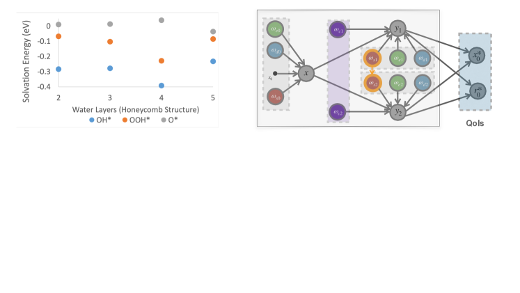
Figure 11: (Left) DFT data for solvation energies $\omega_{s0}$ and $\omega_{si}$ of $x$ and $y_{i}$ respectively, with different water layers. (Right) Based on the left figure, a potential correlation between $\omega_{si}$ is found. We incorporate such a correlation into the graph by adding a new edge between $\omega_{si}$ (orange edge) into the existing graph in Figure 7 (b). The two energies $y_{1}$ and $y_{2}$ are now not conditionally independent given $x$. However, by using (61), the model sensitivity indices $I^{\pm}(x_{O^{\ast}}^{P},P;\mathcal{D}^{\eta_{s2}}_{s2})$ are very small compared to the QoI $\mathbb{E}_{P}[x_{O^{\ast}}^{P}]$
(here the index in (60) is normalized by the QoI) implying that we can ignore the proposed graph connection


The KL divergence between the Gaussian Bayesian networks $P$ and $Q$ of Figure 7 (b) and Figure 11 respectively is given by



(89)

$$R(Q\|P)
=
\int\log\frac{q(\omega_{s2}|\omega_{s1})}{p(\omega_{s2})}q(\omega_{s2}|\omega_{s1})q(\omega_{s1})ds_{2}ds_{1}$$





and serves as a surrogate for the model misspecification $\eta_{s2}$. Using gaussianity $\eta_{s2}=0.9173$, and by Theorem 3.2,
$I^{\pm}(x_{O^{\ast}}^{P},P;\mathcal{D}^{\eta_{s2}}_{s2})=\pm 0.0928$. The latter value is very small compared to the QoI $\mathbb{E}_{P}[x_{O^{\ast}}^{P}]=2.0434$. Thus, we may safely ignore the correlation between $\omega_{s1}$ and $\omega_{s2}$. Therefore, no further model improvement is necessary and we can retain the (simpler) baseline Bayesian network of Figure 7 (b).



8 Conclusions


In this paper, we developed information-theoretic, robust uncertainty quantification methods and non-parametric stress tests for Bayesian networks, which allowed us to assess the effect and the propagation through the graph of multi-sourced model uncertainties to the quantities of interest. These quantification methods also allowed us to rank these sources of uncertainty and correct the graphical model by targeting the most influential components with respect to the quantities of interest.
However, one of the challenges we did not discuss in depth here is the selection of the probabilistic metric or divergence $d$ in the formulation of robust uncertainty quantification, e.g. in the definition of model uncertainty indices (3). In this paper we selected
the KL divergence to define the ambiguity sets (2)
since it allowed us to obtain easily computable and scalable model uncertainty indices.
However, for Bayesian networks with vastly different graphical structures e.g. an alternative model with more vertices than the baseline, the choice of KL is not suitable
due to the lack of absolute continuity between the baseline and the alternative model. In such cases, new divergences could be considered e.g. Wasserstein metrics already studied in the DRO literature [53, 12] or their Integral Probability Metrics (IPM) generalization [55];
alternatively we can consider various interpolations of divergences and IPMs studied recently in the machine learning literature such as
[30, 23, 6, 32] and references therein.
For instance, the recently introduced $(f,\Gamma)$-divergences [6] are interpolations of $f$-divergences and IPMs that combine advantageous features of both,
such as the capability to handle heavy-tailed data (property inherited from $f$-divergences) and to compare non-absolutely continuous distributions (inherited from IPMs).
An additional issue that we touched upon here when we discussed model sensitivity indices is the need for divergences to be able to isolate
sources of uncertainty on localized parts of the graphical model in the spirit of “divide and conquer”. In that respect concepts of sub-additivity of divergences for PGMs can be essential as discussed in related recent literature
[18, 23].


Acknowledgments.
The research of P.B. was supported by the Air Force Office of Scientific Research (AFOSR) under the grant FA-9550-18-1-0214. The research of J.F. was partially supported by the Defense Advanced Research Projects Agency (DARPA) EQUiPS program under the grant W911NF1520122.
The research of M. K. and L. R.-B. was partially supported by
by the Air Force Office of Scientific Research (AFOSR) under the grant FA-9550-18-1-0214
and by
the National Science Foundation (NSF) under
NSF TRIPODS CISE-1934846 and the grant DMS-2008970.




Appendix A Background on Model Uncertainty



A.1 Mathematical formulation of model uncertainty


We can formulate mathematically model uncertainty by constructing (non-parametric) families ${\mathcal{Q}}$ of alternative models $Q$ to compare to a baseline model $P$ which is computationally tractable and inferred from data, and believed to be a good approximation for the physical model of $X$, while the “true”, intractable, partially unknown model $Q^{*}$ should belong to $\mathcal{Q}$; for this reason we refer to ${\mathcal{Q}}$ as the ambiguity set, typically defined as a neighborhood of models around the baseline $P$:



(90)

$$\mathcal{Q}=\mathcal{D}^{\eta}=\big{\{}Q:d(Q,P)\leq\eta\big{\}}\,,$$



where $\eta>0$ corresponds to the size of the ambiguity set and $d=d(Q,P)$ denotes a probability metric or divergence (see Figure 12 (Left) for the schematic depiction where $d$ is the Kullback Leibler (KL) divergence (aka relative entropy) $R(Q\|P)$, [16]). The next natural mathematical goal is to assess the baseline model and understand the resulting biases for QoIs $f$ when we use $P$ for predictions instead of the true model $Q^{*}\in\mathcal{Q}$. As we see later, the free energies $f=-\Delta G_{i}$ are considered as QoIs for the ORR PGM (see Section 7).






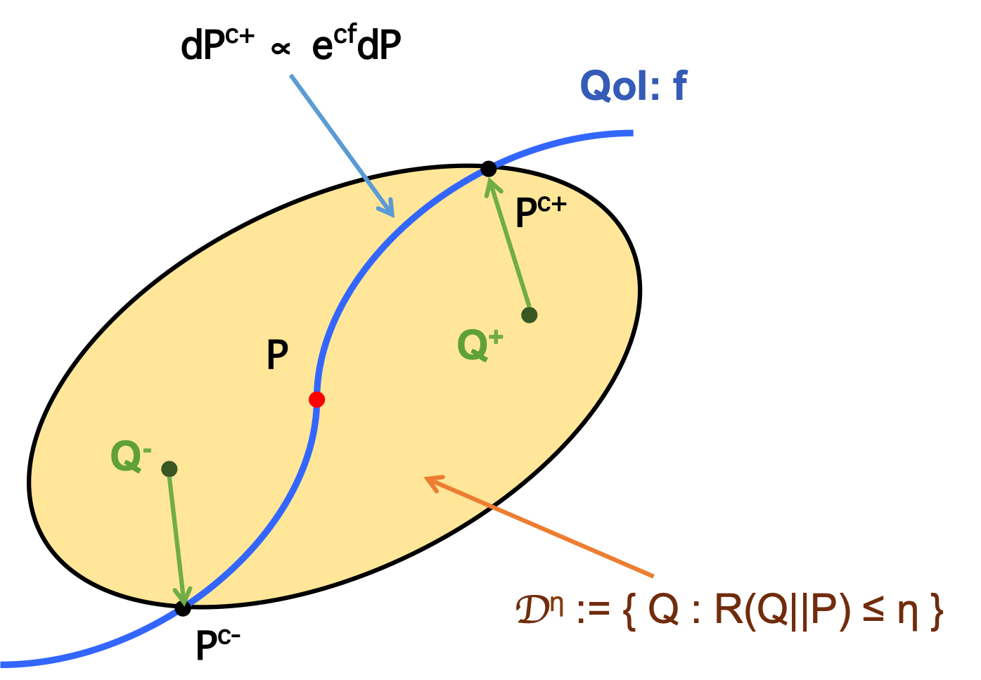
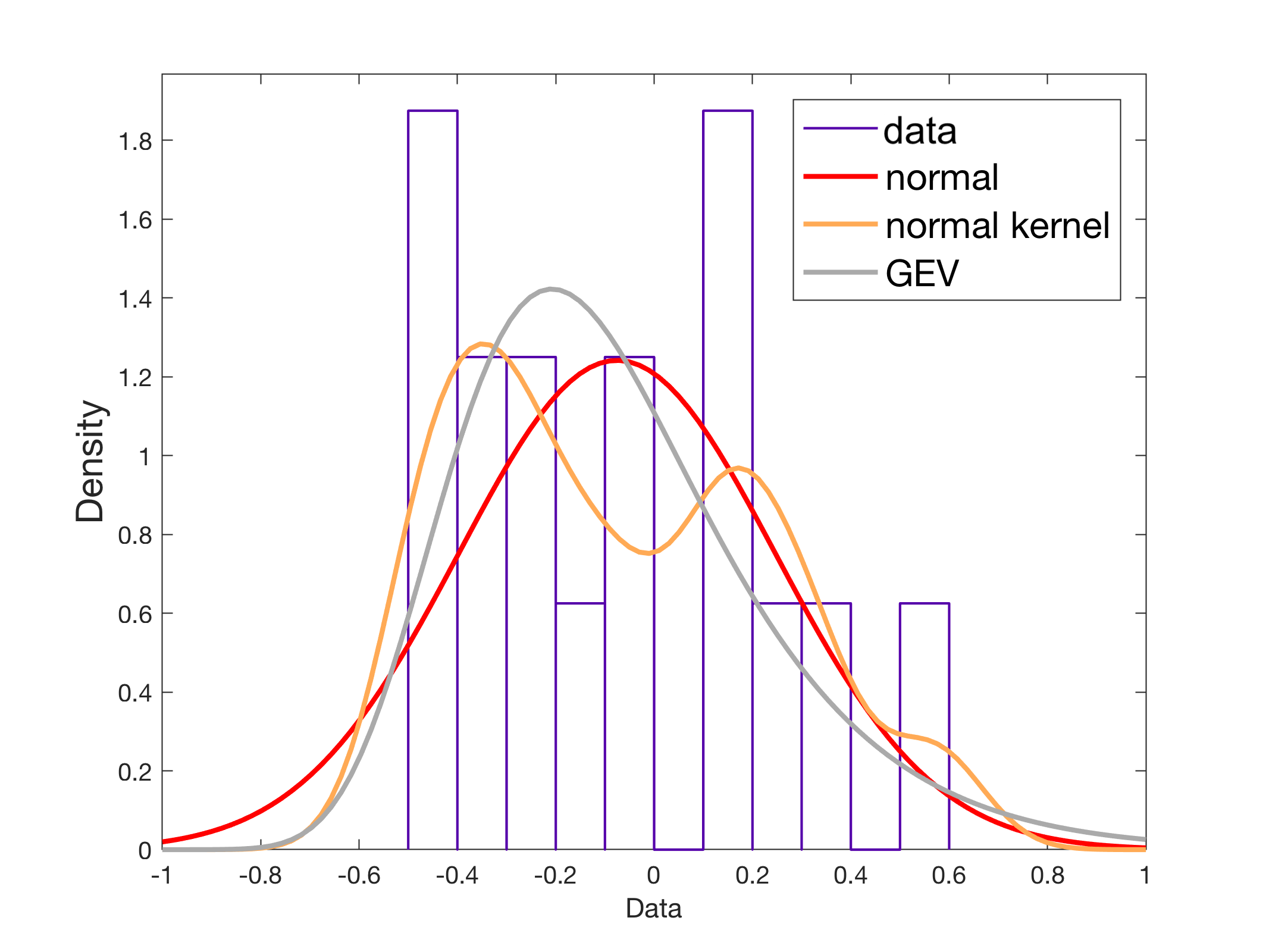
Figure 12: (Left) The schematic illustration of the ambiguity set (non-parametric family of models) given by (90) with $d$ being the KL Divergence $R(Q\|P)$; the blue line represents a parametric family; $Q^{\pm}$ are the probability measures that the UQ indices/bounds $I^{\pm}$ with respect to QoI $f$ are attained and are provided by (93) i.e. tightness of the bounds. (Right) Three probabilistic models with different CPDs for sparse data of a ORR PGM vertex $\omega_{d0}$: the red curve is used to build a baseline Gaussian model denoted by $P$, the gray curve is another parametric model (Generalized Extreme Value (GEV) distribution) which fits the data better, and the yellow curve is a non-parametric model (Kernel Density Estimation (KDE) with normal kernel). 


We define the predictive uncertainty (or bias) for the QoI $f$ when using the baseline model $P$ instead of any alternative model $Q\in\mathcal{Q}$ as the two worst case scenarios:



(91)

$$I^{\pm}(f,P;\mathcal{Q}):=\underset{Q\in\mathcal{Q}}{\mathrm{sup/inf}}\ \{\mathbb{E}_{Q}\left[f\right]-\mathbb{E}_{P}\left[f\right]\}$$



where $\mathbb{E}_{Q}\left[f\right]$ denotes the expected value of the QoI $f$. Therefore, (91) provides a robust performance guarantee for the predictions of the baseline model $P$ for the QoI $f$ within
the ambiguity set $\mathcal{Q}$. This robust perspective for general probabilistic models $P$ is also known in Operations Research as Distributionally Robust Optimization (DRO), e.g.
[17, 33, 74, 44, 29, 49, 53, 75, 12], where optimal-transport (Wasserstein) metrics were recently proposed for (90). Note that the predictive uncertainty represents the robustness of the model $P$ with respect to $\mathcal{Q}$, i.e. all the biases between the predictions of $f$ with $Q\in\mathcal{Q}$ and $P$ are bounded by the predictive uncertainty.




A.2 Existing results on model uncertainty


While the definition (91) is rather natural and intuitive, at least based on the model uncertainty challenge depicted in Figure 12 (Left), it is not obvious that it is practically computable.
However it becomes tractable if we use for metric $d$ in (90) the KL divergence
$R(Q\|P)$. Accordingly, $\eta$ is a measure of the confidence we put in the baseline model $P$ measured using KL divergence.
In recent work [15, 21, 37, 47], it has been shown that $I^{\pm}(f,P;\mathcal{D}^{\eta})$ (an infinite dimensional optimization problem) can be directly computable by a one dimensional optimization problem:



(92)

$$\quad\quad I^{\pm}(f,P;{\mathcal{D}}^{\eta})=\pm\inf_{c>0}\Big{[}\frac{1}{c}\log\int e^{\pm c(f-\mathbb{E}_{P}\left[f\right])}P(dx)+\frac{\eta}{c}\Big{]}=\mathbb{E}_{Q^{\pm}}\left[f\right]-\mathbb{E}_{P}\left[f\right]\,.$$



which is derived by using the Gibbs variational principle [21] for KL divergence. In the first equality of this formula we recognize two ingredients: $\eta$ is model uncertainty from (90) while the Moment Generating Function (MGF) $\int e^{\pm cf}P(dx)$ encodes the QoI $f$ at the baseline model $P$. In [21, 37, 47] techniques are developed to compute (exactly or approximately via asymptotics [21]) as well as provide explicitly upper and lower bounds on $I^{\pm}(f,P;{\mathcal{D}}^{\eta})$ in terms of concentration inequalities [37]. A key point in (92) is that the parameter $\eta$ is not necessarily small, allowing global & non-parametric sensitivity analysis.


Moreover, in [37] the authors have proven that the second equality of (92) holds. In fact, this shows that $I^{\pm}(f,P;{\mathcal{D}}^{\eta})$ is also tight, i.e when the sup and inf in (91) are attained by appropriate measures $Q^{\pm}$. Formally, the authors have shown that there exist $0<\eta_{\pm}\leq\infty$, such that for any $\eta\leq\eta_{\pm}$, $Q^{\pm}(\cdot)=Q^{\pm}(\cdot\;;\pm c_{\pm})$ depend on $\eta$ and are given by



(93)

$$dQ^{\pm}=\frac{e^{\pm c_{\pm}f}}{\mathbb{E}_{P}\left[e^{\pm c_{\pm}f}\right]}\ dP$$



where $c_{\pm}\equiv c_{\pm}(\eta)$ are the unique solutions of



(94)

$$R(Q^{\pm}\|P)=\eta.$$







A.3 Some fundamental Lemmas


In this subsection, we include Lemma A.1 and A.2 for completeness of the background presentation. These results were proved in [21, 22, 37]
and we present them here for the convenience of the reader.



Lemma A.1.


Let $P$ be a probability measure and let $f(X)$ be such that its MGF is finite in a neighborhood of the origin. Then for any $Q$ with $R(Q||P)<\infty$, we have



(95)

$$-\inf_{c>0}\Big{[}\frac{1}{c}\log\mathbb{E}_{P}\left[e^{-c\bar{f}(X)}\right]+\frac{\eta}{c}\Big{]}\leq\mathbb{E}_{Q}\left[f(X)\right]-\mathbb{E}_{P}\left[f(X)\right]\leq\inf_{c>0}\Big{[}\frac{1}{c}\log\mathbb{E}_{P}\left[e^{c\bar{f}(X)}\right]+\frac{\eta}{c}\Big{]}$$







Proof of Lemma A.1. For any general QoI $f(X)$ which has finite moment generating function (MGF), $\mathbb{E}_{P}\left[e^{\pm c\bar{f}(X)}\right]:=\mathbb{E}_{P}\left[e^{c(f(X)-\mathbb{E}_{P}\left[f(X)\right])}\right]$, in a neighborhood of the origin, there is a known fact in statistics and large deviation theory [20, 21] that



(96)

$$\log\mathbb{E}_{P}\left[e^{f(X)}\right]=\sup_{Q\ll P}\{\mathbb{E}_{Q}\left[f(X)\right]-R(Q||P)\}\ .$$



Changing $f(X)$ to $c\bar{f}(X)=c(f(X)-\mathbb{E}_{P}\left[f(X)\right])$, we get



(97)

$$\mathbb{E}_{P}\left[e^{\pm c\bar{f}(X)}\right]=\sup_{Q\ll P}\{c(\mathbb{E}_{Q}\left[f(X)\right]-\mathbb{E}_{P}\left[f(X)\right])-R(Q||P)\}$$



which gives us the following upper and lower bounds with $c>0$,



(98)

$$-\inf_{c>0}\Big{[}\frac{1}{c}\log\mathbb{E}_{P}\left[e^{-c\bar{f}(X)}\right]+\frac{\eta}{c}\Big{]}\leq\mathbb{E}_{Q}\left[f(X)\right]-\mathbb{E}_{P}\left[f(X)\right]\leq\inf_{c>0}\Big{[}\frac{1}{c}\log\mathbb{E}_{P}\left[e^{c\bar{f}(X)}\right]+\frac{\eta}{c}\Big{]}$$



where $\eta=R(Q||P)$.



Lemma A.2.


Suppose $(d_{-},d_{+})$ is the largest open set such that cumulant generating function $\Lambda(c)=\log\mathbb{E}_{P}\left[e^{c\bar{f}(X)}\right]<\infty$ for all $c\in(d_{-},d_{+})$.


 

For any $\eta\geq 0$ the optimization problems




$$\inf_{c>0}\frac{\Lambda(\pm c)+\eta}{c}$$



have unique minimizers $c_{\pm}\in[0,\pm d_{\pm}]$.
Let $\eta_{\pm}$ be defined by




$$\eta_{\pm}=\lim_{c\nearrow\pm d_{\pm}}\pm c\Lambda^{\prime}(\pm c)-\Lambda(\pm c)\,.$$



Then
the minimizers $c_{\pm}=c_{\pm}(\eta)$
are finite for $\eta<\eta_{\pm}$ and $c_{\pm}(\eta)=\pm d_{\pm}$ if $\eta\geq\eta_{\pm}$.



 

If $c_{\pm}(\eta)<\pm d_{\pm}$ then



(99)

$$\frac{\Lambda(\pm c_{\pm})+\eta}{c_{\pm}}=\inf_{c>0}\frac{\Lambda(\pm c)+\eta}{c}\,=\,\pm\Lambda^{\prime}(\pm c_{\pm})=\pm\left(\mathbb{E}_{P_{\pm c_{\pm}}}[f]-\mathbb{E}_{P}[f]\right)\,,$$



where $c_{\pm}(\eta)$ is strictly increasing in $\eta$ and is determined by the
equation



(100)

$$R\left({P_{\pm c_{\pm}}}{\,||\,}{P}\right)=\eta\,.$$






 

$\eta_{\pm}$ is finite in two distinct cases.


 

If $\pm d_{\pm}<\infty$ (in which case $g$ must be unbounded above/below) $\eta_{\pm}$ is finite if $\lim_{c\to\pm d_{\pm}}\Lambda(\pm c):=\Lambda(d_{\pm})<\infty$ and $\lim_{c\to\pm d_{\pm}}\pm\Lambda^{\prime}(\pm c):=\pm\Lambda^{\prime}(d_{\pm})<\infty$, and for $\eta\geq\eta_{\pm}$ we have



(101)

$$\inf_{c>0}\frac{\Lambda(\pm c)+\eta}{c}=\frac{\Lambda(d_{\pm})+\eta}{\pm d_{\pm}}=\pm\left(\mathbb{E}_{P_{d_{\pm}}}[f]-\mathbb{E}_{P}[f]\right)+\frac{\eta-\eta_{\pm}}{\pm d_{\pm}}\,.$$






 

If $\pm d_{\pm}=\infty$ and $\eta_{\pm}$ is finite then $f$ is $P$-a.s. bounded above/below and for $\eta\geq\eta_{\pm}$ we have



(102)

$$\inf_{c>0}\frac{\Lambda(\pm c)+\eta}{c}=\mathrm{ess\,sup}_{x\in\mathcal{X}}\{\pm(f(x)-\mathbb{E}_{P}\left[f(X)\right])\}\,.$$













Proof of the Lemma A.2.
For notational ease, in the proof, let
us set $\Lambda(c)=\log\mathbb{E}_{P}\left[e^{c\bar{f}(X)}\right]$ so that the UQ indices is




$$I^{\pm}(f(X),P;\mathcal{D}^{\eta})=\inf_{c>0}\left\{\frac{\Lambda(\pm c)+\eta}{c}\,\right\}$$



Note that $\Lambda(c)$ is convex function which we assume to
be finite on an interval $(d_{-},d_{+})$ with $d_{-}<0<d+$. On that interval $\Lambda(c)$ is infinitely differentiable and strictly convex. Since we centered the QoI we have $\Lambda(0)=\Lambda^{\prime}(0)=0$ and $\Lambda^{\prime\prime}(0)=\operatorname{Var}_{P}(f)$.


First note that it is enough to prove the result for $\Lambda(c)$ since the result for $\Lambda(-c)$ is obtained by replacing $f$ by $-f$. We also use the notation $\tilde{f}_{+}=\mathrm{ess\,sup}\{f(x)-\mathbb{E}_{P}\left[f(X)\right]\}$.


We first claim that automatically




$$\Lambda(d_{+})=\lim_{c\nearrow d_{+}}\Lambda(c),$$



where $\Lambda(d_{+})$ may be infinite. By monotone convergence




$$\mathbb{E}_{P}[1_{\{\tilde{f}\geq 0\}}e^{c\tilde{f}}]\nearrow\mathbb{E}_{P}[1_{\{\tilde{f}\geq 0\}}e^{d_{+}\tilde{f}}]$$



as $c\nearrow d_{+}$. By dominated convergence




$$\mathbb{E}_{P}[1_{\{\tilde{f}<0\}}e^{c\tilde{f}}]\searrow\mathbb{E}_{P}[1_{\{\tilde{f}<0\}}e^{d_{+}\tilde{f}}]$$



as $c\nearrow d_{+}$, and the claim follows. A very similar argument shows that $\Lambda^{\prime}(c)$ also has a limit as $c\nearrow d_{+}$.


Let



(103)

$$B(c;\eta)=\frac{\Lambda(c)+\eta}{c}.$$



We divide into cases.




 

$\tilde{f}_{+}<\infty$. In this case $\Lambda^{\prime}(c)\nearrow\tilde{f}_{+}<\infty$
as $c\rightarrow\infty$ and $\Lambda^{\prime}(0)<\tilde{f}_{+}$. If $\eta=0$ then the
infimum is $\Lambda^{\prime}(0)$ and attained at $c_{+}=0$ since $\Lambda(c)/c$ is an increasing function. If $\eta>0$ then




$$B^{\prime}(c;\eta)=\frac{c\Lambda^{\prime}(c)-\Lambda(c)-\eta}{c^{2}}$$



for $c\geq 0$. The function $c\Lambda^{\prime}(c)-\Lambda(c)$ strictly
increases from $0$ at $c=0$ to some limit $\eta_{+}>0$ at $c=\infty$,
and the minimizer is at the unique finite root of $c\Lambda^{\prime}(c)-\Lambda(c)=\eta$ for $\eta<\eta_{+}$ and $c_{+}=\infty$ for $\eta\geq\eta_{+}$.



 

$\tilde{f}_{+}=\infty$. In this case there are two subcases.




 

$d_{+}=\infty$. In this case since $\tilde{f}_{+}=\infty$ we have $\Lambda^{\prime}(c)\nearrow\infty$ as $c\rightarrow\infty$ and $c\Lambda^{\prime}(c)-\Lambda(c)\rightarrow\infty$ as $c\rightarrow\infty$. Since
$0\Lambda^{\prime}(0)-\Lambda(0)=0$, in all cases of $\eta\geq 0$ there is a unique root
to $c\Lambda^{\prime}(c)-\Lambda(c)=\eta$ and hence a unique minimizer.



 

$d_{+}<\infty$. We know that $\Lambda^{\prime}(c)$ converges as
$c\nearrow d_{+}$ to a well defined left hand limit which we call
$\Lambda^{\prime}(d_{+})$ (note that this value could be $\infty$). Thus we have
that $c\Lambda^{\prime}(c)-\Lambda(c)$ ranges from $0$ at $c=0$ to
$\eta_{+}=d_{+}\Lambda^{\prime}(d_{+})-\Lambda(d_{+})$. For $\eta\in[0,\eta_{+})$ there is a
unique minimizer in $[0,d_{+})$. For $\eta\geq\eta_{+}$ the unique minimizer is at
$c_{+}=d_{+}$.








To conclude the proof we note that if
$c_{+}<d_{+}$ then an easy computation shows that




$$c_{+}\Lambda^{\prime}(c_{+})-\Lambda(c_{+})=R(P_{c_{+}}\,||\,P)=\eta\,,$$



and thus




$$B(c_{+},\eta)=\Lambda^{\prime}(c_{+})=\mathbb{E}_{P_{c_{+}}}[f]-\mathbb{E}_{P}\left[f(X)\right]$$



which proves (99) and (94). Finally if $d_{+}=\infty$ and $f$ is $P$-a.s. bounded above then the infimum is equal to $\lim_{c\to\infty}\frac{\Lambda(c)}{c}$ and this establishes (102).
If $d_{+}<\infty$ and $\eta_{+}<\infty$ then the bound takes the form (101).





Appendix B A simple example for Bayesian networks



In this example, we focus on the construction of the graph structure and CPDs of the optimal distributions provided by Theorem 2.1 (b) following the strategy of its proof. Note that in the next subsection by assuming
that each $X_{i}$ is linear Gaussian of its parents, we also compute the model uncertainty indices given by (9) in Theorem 2.1 (a). Let us consider a Bayesian network as shown in Figure 2 (a), with density given by



(104)

$$p(x)=p(x_{1})p(x_{2})p(x_{3}|x_{2},x_{1})p(x_{4})p(x_{5}|x_{3})p(x_{6}|x_{4},x_{3})p(x_{7}|x_{6},x_{5})p(x_{8}|x_{6})$$



For a QoI $f(X_{6})$,
the optimizers in Theorem 2.1 (b) are obtained when the CPDs of $X_{5}$, $X_{7}$ and $X_{8}$ are the same with the corresponding CPDs of $P$ as these vertices are not ancestors of $X_{6}$ while



(105)

$$q^{\pm}(x_{6}|x_{\pi_{6}^{Q^{\pm}}})
=
\frac{e^{\pm c_{\pm}f(x_{6})}}{\mathbb{E}_{P_{6|\{4,3\}}}\left[e^{\pm c_{\pm}f(X_{6})}\right]}\cdot p(x_{6}|x_{4},x_{3})$$





where $\pi_{6}^{Q^{\pm}}\equiv\pi_{6}^{P}=\{4,3\}$, then for $i\in\rho_{6}=\{1,2,3,4\}$



(106)

$$q^{\pm}(x_{4}|x_{\pi_{4}^{Q^{\pm}}})
=
\frac{\mathbb{E}_{P_{6|\{4,3\}}}\left[e^{\pm c_{\pm}f(X_{6})}\right]}{\mathbb{E}_{P_{4}}\left[\mathbb{E}_{P_{6|\{4,3\}}}\left[e^{\pm c_{\pm}f(X_{6})}\right]\right]}p(x_{4})$$





since both normalization factors on the numerator and denominator depend on $X_{\pi_{6}}=\{X_{4},X_{3}\}$, so in general, we have $\pi_{4}^{Q^{\pm}}=\pi_{4}^{P}\cup\{3\}=\{3\}$, i.e., there is a new connection $X_{3}\to X_{4}$ in $Q^{\pm}$, and



(107)

$$q^{\pm}(x_{3}|x_{\pi_{3}^{Q^{\pm}}})
=
\frac{\mathbb{E}_{P_{4}}\left[\mathbb{E}_{P_{6|\{4,3\}}}\left[e^{\pm c_{\pm}f(X_{6})}\right]\right]}{\mathbb{E}_{P_{3|\{2,1\}}}\left[\mathbb{E}_{P_{4}}\left[\mathbb{E}_{P_{6|\{4,3\}}}\left[e^{\pm c_{\pm}f(X_{6})}\right]\right]\right]}p(x_{3}|x_{2},x_{1})$$





where $\pi_{3}^{Q^{\pm}}\equiv\pi_{3}^{P}=\{2,1\}$ since the normalization factors do not contain other variables. We can similarly do the same for $X_{2}$ and $X_{1}$ to get the entire structure of $Q^{\pm}$ which has another new connection $X_{1}\to X_{2}$, and the results are shown in Figure 2 (b).


For $A=\{3,6,7\}$, we consider a QoI $f(X_{A})=f(X_{3},X_{6},X_{7})$ and by Theorem 2.1 (a), the following holds:




(108)

$$I^{\pm}(f(X_{3},X_{6},X_{7}),P;\mathcal{D}^{\eta})
=
\pm\inf_{c>0}\Big{[}\frac{1}{c}\log\mathbb{E}_{P_{A}}\left[e^{\pm c\bar{f}(X_{A})}\right]+\frac{\eta}{c}\Big{]}$$







$$=
\mathbb{E}_{Q^{\pm}}\left[f(X_{A})\right]-\mathbb{E}_{P}\left[f(X_{A})\right]$$





where $Q^{\pm}$ are the optimizers with CPDs given by (109)-(116) and




$$\mathbb{E}_{P_{A}}\left[e^{\pm c\bar{f}(X_{A})}\right]=\int e^{\pm c\bar{f}(x_{3},x_{6},x_{7})}\prod_{i=1}^{7}p(x_{i}|x_{\pi_{i}})dx_{i}$$



We recall (12) of Theorem 2.1 (b), and we obtain the CPDs of $Q^{\pm}$ and the new parents of each vertex as follows:



(109)

$$q^{\pm}(x_{8}|x_{\pi_{8}^{Q^{\pm}}})\equiv p(x_{8}|x_{\pi_{8}^{Q^{\pm}}})\equiv p(x_{8}|x_{6})$$






(110)

$$q^{\pm}(x_{7}|x_{\pi_{7}^{Q^{\pm}}})
=
\frac{e^{\pm c_{\pm}f(x_{7},x_{6},x_{3})}}{\mathbb{E}_{p_{7|\{6,5\}}}\left[e^{\pm c_{\pm}f(X_{7},X_{6},X_{3})}\right]}\cdot p(x_{7}|x_{6},x_{5})$$





with $\pi_{7}^{P}\subset\pi_{7}^{Q^{\pm}}=\pi_{7}^{P}\cup\{3\}=\{6,5,3\}$. Let $\{l_{1},\dots,l_{6}\}\equiv\rho_{3}^{P}\cup\rho_{6}^{P}\cup\rho_{7}^{P}\cup\{3,6\}=\{1,2,3,4,5,6\}$. We start with $X_{6}$ as it is indexed by the $\max\{l_{j}:j\in 1,\dots,6\}$



(111)

$$q^{\pm}(x_{6}|x_{\pi_{6}^{Q^{\pm}}})
=
\frac{\mathbb{E}_{P_{7|\pi_{7}}}[e^{\pm c_{\pm}f(X_{A})}]}{\mathbb{E}_{P_{6|\pi_{6}},P_{7|\pi_{7}}}[e^{\pm c_{\pm}f(X_{7},X_{6},X_{3})}]}\cdot p(x_{6}|x_{4},x_{3})$$





with $\pi_{6}^{P}\subset\pi_{6}^{Q^{\pm}}\subset\pi_{6}^{P}\cup\{5\}=\{3,4,5\}$. Similarly, the CPD of $X_{1},\cdots,X_{5}$ are given by



(112)

$$q^{\pm}(x_{5}|x_{\pi_{5}^{Q^{\pm}}})
=\frac{\mathbb{E}_{P_{6|\pi_{6}},P_{7|\pi_{7}}}[e^{\pm c_{\pm}f(X_{A})}]}{\mathbb{E}_{P_{5|\pi_{5}},P_{6|\pi_{6}},P_{7|\pi_{7}}}[e^{\pm c_{\pm}f(X_{7},X_{6},X_{3})}]}\cdot p(x_{5}|x_{3}),$$




(113)

$$q^{\pm}(x_{4}|x_{\pi_{4}^{Q^{\pm}}})
=\frac{\mathbb{E}_{P_{5|\pi_{5}},P_{6|\pi_{6}},P_{7|\pi_{7}}}[e^{\pm c_{\pm}f(X_{A})}]}{\mathbb{E}_{P_{4|\pi_{4}},P_{5|\pi_{5}},P_{6|\pi_{6}},P_{7|\pi_{7}}}[e^{\pm c_{\pm}f(X_{7},X_{6},X_{3})}]}\cdot p(x_{4}),$$




(114)

$$q^{\pm}(x_{3}|x_{\pi_{3}^{q^{\pm}}})
=\frac{\mathbb{E}_{P_{4|\pi_{4}},\cdots,P_{7|\pi_{7}}}[e^{\pm c_{\pm}f(X_{A})}]}{\mathbb{E}_{P_{3|\pi_{3}},\cdots,P_{7|\pi_{7}}}[e^{\pm c_{\pm}f(X_{7},X_{6},X_{3})}]}\cdot p(x_{3}|x_{2},x_{1}),$$




(115)

$$q^{\pm}(x_{2}|x_{\pi_{2}^{q^{\pm}}})
=\frac{\mathbb{E}_{P_{3|\pi_{3}},\cdots,P_{7|\pi_{7}}}[e^{\pm c_{\pm}f(X_{A})}]}{\mathbb{E}_{P_{2|\pi_{2}},\cdots,P_{7|\pi_{7}}}[e^{\pm c_{\pm}f(X_{7},X_{6},X_{3})}]}\cdot p(x_{2}|x_{1}),$$




(116)

$$q^{\pm}(x_{1}|x_{\pi_{1}^{q^{\pm}}})
=\frac{\mathbb{E}_{P_{2|\pi_{2}},\cdots,P_{7|\pi_{7}}}[e^{\pm c_{\pm}f(X_{A})}]}{\mathbb{E}_{P_{1|\pi_{1}},\cdots,P_{7|\pi_{7}}}[e^{\pm c_{\pm}f(X_{7},X_{6},X_{3})}]}\cdot p(x_{1}),$$




where the expectations involved in the above formulas are given by (8). The corresponding structures are:



(117)

$$\qquad\pi_{5}^{P}\subset\pi_{5}^{Q^{\pm}}\subset\pi_{5}^{P}\cup\{4\}=\{3,4\}$$



(118)

$$\qquad\pi_{4}^{P}\subset\pi_{4}^{Q^{\pm}}\subset\pi_{4}^{P}\cup\{3\}=\{3\}$$



(119)

$$\qquad\pi_{3}^{P}\subset\pi_{3}^{Q^{\pm}}\subset\pi_{3}^{P}=\{1,2\}$$



(120)

$$\qquad\pi_{2}^{P}\subset\pi_{2}^{Q^{\pm}}\subset\pi_{2}^{P}\cup\{1\}=\{1\}$$



(121)

$$\qquad\pi_{1}^{Q^{\pm}}=\pi_{1}^{P}=\emptyset.$$



As a result, the structure of the associated graph to $Q^{\pm}$ may change and in particular, the vertices-with potentially extra parents-are $X_{2},X_{4},X_{5},X_{6}$ and $X_{7}$ as illustrated in Figure 2 (c).




Appendix C A simple example for Gaussian Bayesian networks



[Continuation of Example B] We assume that CPDs of Example B with graph structure as in Figure 2, (a) are given by:




$$\begin{aligned} p(x_{8}|x_{6})&=\mathcal{N}(\beta_{80}+\beta_{86}x_{6},\sigma_{8}^{2})\\
p(x_{7}|x_{6},x_{5})&=\mathcal{N}(\beta_{70}+\beta_{76}x_{6}+\beta_{75}x_{5},\sigma_{7}^{2})\\
p(x_{6}|x_{4},x_{3})&=\mathcal{N}(\beta_{60}+\beta_{64}x_{4}+\beta_{63}x_{3},\sigma_{6}^{2})\\
p(x_{5}|x_{3})&=\mathcal{N}(\beta_{50}+\beta_{53}x_{3},\sigma_{5}^{2})\end{aligned}\quad\begin{aligned} p(x_{4})&=\mathcal{N}(\beta_{40},\sigma_{4}^{2})\\
p(x_{3}|x_{2},x_{1})&=\mathcal{N}(\beta_{30}+\beta_{32}x_{2}+\beta_{31}x_{1},\sigma_{3}^{2})\\
p(x_{2})&=\mathcal{N}(\beta_{20},\sigma_{2}^{2})\\
p(x_{1})&=\mathcal{N}(\beta_{10},\sigma_{1}^{2})\end{aligned}$$



Then, $p(x)=\mathcal{N}(\mu,\mathcal{C})$, [48, Theorem 7.3]. As before, the QoI depends on $X_{6}$ and for simplicity, we consider $f(X_{6})=X_{6}$. For $c>0$, we compute the MGF of $f$ with respect to $P$:




$$\mathbb{E}_{P}\left[e^{\pm c\bar{f}(X_{6})}\right]=\exp\left\{\frac{c^{2}}{2}\left(\sigma_{6}^{2}+\beta_{64}^{2}\sigma_{4}^{2}+\beta_{63}^{2}\sigma_{3}^{2}+\beta_{63}^{2}\beta_{32}^{2}\sigma_{2}^{2}+\beta_{63}^{2}\beta_{31}^{2}\sigma_{1}^{2}\right)\right\}\equiv e^{\frac{c^{2}}{2}\mathcal{C}_{66}}$$



where $\mathcal{C}_{66}=\sigma_{6}^{2}+\beta_{64}^{2}\sigma_{4}^{2}+\beta_{63}^{2}\sigma_{3}^{2}+\beta_{63}^{2}\beta_{32}^{2}\sigma_{2}^{2}+\beta_{63}^{2}\beta_{31}^{2}\sigma_{1}^{2}$ since $\mathbb{E}_{P}\left[X_{6}\right]=\beta_{60}+\beta_{64}\beta_{40}+\beta_{63}\beta_{30}+\beta_{63}\beta_{32}\beta_{20}+\beta_{63}\beta_{31}\beta_{10}$. We minimize (9) in Theorem 2.1 with respect to $c$:




$$I^{\pm}(f(X_{6}),P;\mathcal{D}^{\eta})
=
\pm\inf_{c>0}\Big{[}\frac{1}{c}\log\mathbb{E}_{P}\left[e^{\pm c\bar{f}(X_{6})}\right]+\frac{\eta}{c}\Big{]}=\pm\inf_{c>0}\Big{[}c\,\mathcal{C}_{66}+\frac{\eta}{c}\Big{]}$$





which in turn gives us the optimizer $c=\sqrt{\frac{\eta}{\mathcal{C}_{66}}}$, and thus



(122)

$$I^{\pm}(f(X_{6}),P;\mathcal{D}^{\eta})=\pm\sqrt{2\mathcal{C}_{66}\eta}=\pm\sqrt{2(\sigma_{6}^{2}+\beta_{64}^{2}\sigma_{4}^{2}+\beta_{63}^{2}\sigma_{3}^{2}+\beta_{63}^{2}\beta_{32}^{2}\sigma_{2}^{2}++\beta_{63}^{2}\beta_{31}^{2}\sigma_{1}^{2})\eta}$$



By (12), the optimizers in Theorem 2.1 are obtained when



(123)

$$q^{\pm}(x_{i}|x_{\pi^{Q^{\pm}}_{i}})=p(x_{i}|x_{\pi_{i}})=\mathcal{N}(\beta_{i0}+\beta_{i}^{T}x_{\pi_{i}},\sigma_{i}^{2})$$



for $i=5,7,8$, since they are not ancestors of $X_{6}$, and by recalling (105)-(107) we further compute the CPDs of the remaining vertices as follows: Since $f(X_{6})=X_{6}$ is linear and all random variables are linearly depended on their parents, we appropriately pair the factor $e^{\pm c_{\pm}x_{6}}$ with the exponential of the Gaussian CPD $p(x_{6}|x_{\pi_{6}^{P}})$ and we get a new quadratic term in the exponential as well as a term which linearly depends on the parents of $X_{6}$. The latter term is canceled out with the corresponding one in the normalizing factor $\mathbb{E}_{P_{6|\pi_{6}^{P}}}\left[e^{\pm c_{\pm}X_{6}}\right]$ as the parents of $X_{6}$ are given. Precisely,





$$q^{\pm}(x_{6}|x_{\pi_{6}^{Q^{\pm}}})
=
\frac{e^{\pm c_{\pm}x_{6}}}{\mathbb{E}_{P_{6|\pi_{6}^{P}}}\left[e^{\pm c_{\pm}X_{6}}\right]}\cdot p(x_{6}|x_{\pi_{6}^{P}})$$







$$=
\frac{\exp\left\{-\frac{(x_{6}-\beta_{60}-\beta_{64}x_{4}-\beta_{63}x_{2}\mp c_{\pm}\sigma_{6}^{2})^{2}}{2\sigma_{6}^{2}}\pm c_{\pm}(\beta_{64}x_{4}+\beta_{63}x_{3})\right\}}{\int_{\mathcal{X}_{6}}\exp\left\{-\frac{(x_{6}-\beta_{60}-\beta_{64}x_{4}-\beta_{63}x_{2}\mp c_{\pm}\sigma_{6}^{2})^{2}}{2\sigma_{6}^{2}}\pm c_{\pm}(\beta_{64}x_{4}+\beta_{63}x_{3})\right\}dx_{6}}$$





Thus,



(124)

$$\;\;\;\;\;\;\;\;q^{\pm}(x_{6}|x_{\pi_{6}^{Q^{\pm}}})=\mathcal{N}\left(\beta_{60}+\beta_{64}x_{4}+\beta_{63}x_{3}\pm c_{\pm}\sigma_{6}^{2},\sigma_{6}^{2}\right),\quad\pi_{6}^{Q^{\pm}}\equiv\pi_{6}^{P}=\{4,3\}.$$



Similarly, for $4\in\rho_{6}$ $=\{4,3,2,1\}$




$$q^{\pm}(x_{4}|x_{\pi_{4}^{Q^{\pm}}})=\frac{\mathbb{E}_{P_{6|\{4,3\}}}\left[e^{\pm c_{\pm}X_{6}}\right]}{\mathbb{E}_{P_{4}}\left[\mathbb{E}_{P_{6|\{4,3\}}}\left[e^{\pm c_{\pm}X_{6}}\right]\right]}p(x_{4})=\frac{e^{-\frac{(x_{4}-\beta_{40}\mp c_{\pm}\beta_{43}\sigma_{4}^{2})^{2}}{2\sigma_{4}^{2}}}e^{\pm c_{\pm}(\beta_{63}x_{3})}}{\int_{\mathcal{X}_{4}}e^{-\frac{(x_{4}-\beta_{40}\mp c_{\pm}\beta_{43}\sigma_{4}^{2})^{2}}{2\sigma_{4}^{2}}}\ dx_{4}\ e^{\pm c_{\pm}(\beta_{63}x_{3})}}$$



Using same the same argument as before, we get



(125)

$$q^{\pm}(x_{4}|x_{\pi_{4}^{Q^{\pm}}})=\mathcal{N}\left(\beta_{40}\pm c_{\pm}\sigma_{4}^{2},\sigma_{4}^{2}\right),\qquad\pi_{4}^{Q^{\pm}}\equiv\pi_{4}^{P}=\emptyset.$$



Furthermore,




(126)

$$q^{\pm}(x_{3}|x_{\pi_{3}^{Q^{\pm}}})
=\mathcal{N}\left(\beta_{30}+\beta_{32}x_{2}+\beta_{31}x_{1}\pm c_{\pm}\sigma_{3}^{2},\sigma_{3}^{2}\right),\qquad
\pi_{3}^{Q^{\pm}}\equiv\pi_{3}^{P}=\{1,2\}$$





(127)

$$q^{\pm}(x_{2}|x_{\pi_{2}^{Q^{\pm}}})
=\mathcal{N}\left(\beta_{20}\pm c_{\pm}\sigma_{2}^{2},\sigma_{2}^{2}\right),\qquad
\pi_{2}^{Q^{\pm}}\equiv\pi_{2}^{P}=\emptyset$$





(128)

$$q^{\pm}(x_{1}|x_{\pi_{1}^{Q^{\pm}}})
=\mathcal{N}\left(\beta_{10}\pm c_{\pm}\sigma_{1}^{2},\sigma_{1}^{2}\right),\qquad
\pi_{1}^{Q^{\pm}}\equiv\pi_{1}^{P}=\emptyset.$$





By using the equation $\pm c_{\pm}\mathbb{E}_{Q^{\pm}}\left[X_{6}\right]-\log\mathbb{E}_{P}\left[e^{\pm c_{\pm}X_{6}}\right]=\eta$, the parameters $c_{\pm}$ are given by



(129)

$$c_{\pm}=\pm\sqrt{\frac{2\eta}{\mathcal{C}_{66}}}=\pm\sqrt{\frac{2\eta}{\sigma_{6}^{2}+\beta_{64}^{2}\sigma_{4}^{2}+\beta_{63}^{2}\sigma_{3}^{2}+\beta_{63}^{2}\beta_{32}^{2}\sigma_{2}^{2}+\beta_{63}^{2}\beta_{31}^{2}\sigma_{1}^{2}}}$$




[Computation of $F$ for Example C]  For Example C, we compute $F(x_{3},\rho_{3})$ with $f(X_{6})=X_{6}$ and $l=3$ (and thus $\rho_{6}=\{1,2,3,4\}$ and $\rho_{3}=\{1,2\}$) as







$$F(x_{3},x^{P}_{\rho_{3}})\equiv F(x_{3},x_{2},x_{1})
=
\int_{\mathcal{X}_{\{4,6\}}}x_{6}p(x_{6}|x_{4},x_{3})p(x_{4})dx_{6}dx_{4}$$







$$=
\beta_{60}+\beta_{64}\beta_{40}+\beta_{63}x_{3}=F(x_{3})$$








[Computation of $\beta_{kl}$ and $\tilde{\beta}_{kl}$ for Example C]
Let us now revisit Example C and compute $\beta_{kl}$ and $\tilde{\beta}_{kl}$ of Corollary 3.8 when $l\in\pi_{k}^{P}$, e.g $l=3$ and $l\in\rho_{k}\setminus\pi_{k}$, e.g. $l=2$ respectively. In the first case, $P_{3|\pi_{3}}$ is perturbed under the constraint $R(Q_{3|\pi_{3}^{Q}}\|P_{3|\pi_{3}})\leq\eta_{3}$ or $R(Q_{3|\pi_{3}}\|P_{3|\pi_{3}})\leq\eta_{3}$, i.e. consider $Q\in\mathcal{D}^{\eta_{3}}_{3}$ or $\mathcal{D}^{\eta_{3}}_{3,P}$ and $f(X_{6})=X_{6}$. $F(x_{3},x_{\rho_{3}})$ is given by (C) and by Theorem 3.2, 3.4 and (3.2), we can conclude that



(131)

$$I^{\pm}(f(X_{6}),P;\mathcal{D}_{3}^{\eta_{3}})=I^{\pm}(f(X_{6}),P;\mathcal{D}_{3,P}^{\eta_{3}})=\pm|\beta_{63}|\sqrt{2\sigma_{3}^{2}\eta_{3}}$$



In the second case, $P_{2|\pi_{2}}$ is perturbed under the constraint $R(Q_{2|\pi_{2}^{Q}}\|P_{2|\pi_{2}})\leq\eta_{2}$ or $R(Q_{2|\pi_{2}}\|P_{3|\pi_{2}})\leq\eta_{2}$. We compute $F(x_{2},x_{\rho_{2}})=\beta_{60}+\beta_{64}\beta_{40}+\beta_{63}\beta_{30}+\beta_{63}\beta_{32}x_{2}+\beta_{63}\beta_{31}\beta_{10}=F(x_{2})$ and $\tilde{\beta}_{62}=\beta_{63}\beta_{32}$.




Appendix D Model uncertainty for inhomogeneous Markov chains


We consider the Markov chain models shown in Figure 13, and the QoI $f(X_{k})$. Then we only perturb $P_{l|l-1}$ with $l\leq k$, under the constraint $R(Q_{l|\pi_{l}^{Q}}\|P_{l|l-1})\leq\eta_{l}$. The function $F(x_{l},x_{\rho_{l}^{P}})$ defined in (3.1) depends only on $x_{l}$ and by Theorem 3.2, we have



(132)

$$I^{\pm}(f(X_{k}),P;\mathcal{D}_{l}^{\eta_{l}})=\pm\mathbb{E}_{P_{\{l-1\}}}\left[\inf_{c>0}\Big{[}\frac{1}{c}\log\mathbb{E}_{P_{l|l-1}}\left[e^{\pm c\bar{F}(X_{l},X_{\rho_{l}})}\right]+\frac{\eta_{l}}{c}\Big{]}\right].$$



Since $F(x_{l},x_{\rho_{l}^{P}})=F(x_{l})$ the condition on Theorem 3.4 is satisfied, and therefore we have $I^{\pm}(f(X_{k}),P;\mathcal{D}^{\eta_{l}}_{l,P})=I^{\pm}(f(X_{k}),P;\mathcal{D}_{l}^{\eta_{l}})$. To obtain the optimizers in both Theorem 3.2 and 3.4, we use (33)-(34) and thus



(133)

$$q^{\pm}(x_{i}|x_{i-1})\equiv p(x_{i}|x_{i-1})\qquad\textrm{ for all $i\neq l$}$$



and



(134)

$$q^{\pm}(x_{l}|x_{l-1})=\frac{e^{\pm c_{\pm}(x_{l-1})F(x_{l})}}{\mathbb{E}_{P}\left[e^{\pm c_{\pm}(x_{l-1})F(X_{l})}|x_{l-1}\right]}p(x_{l}|x_{l-1})$$



where $c_{\pm}(x_{l-1})$ are the unique solutions of $R(P^{\pm c_{\pm}}_{l|l-1}\|P_{l|l-1})=\eta_{l}$
for all $x_{l-1}$. Moreover, by perturbing $P_{l|l-1}$, $l>k$, with the constraint




$$R(Q_{l|\pi_{l}^{Q}}\|P_{l|l-1})\leq\eta_{l}\textrm{ or }R(Q_{l|l-1}\|P_{l|l-1})\leq\eta_{l},$$



and by Theorem 3.2 and 3.4, we have $I^{\pm}(f(X_{k}),P;\mathcal{D}_{l}^{\eta_{l}})=I^{\pm}(f(X_{k}),P;\mathcal{D}^{\eta_{l}}_{l,P})=0$. Note that when the ambiguity set is given by (5), it includes also $Q$’s that are non-Markovian. However, the optimizers are inhomogeneous Markov chains and are provided by Theorem 2.1.


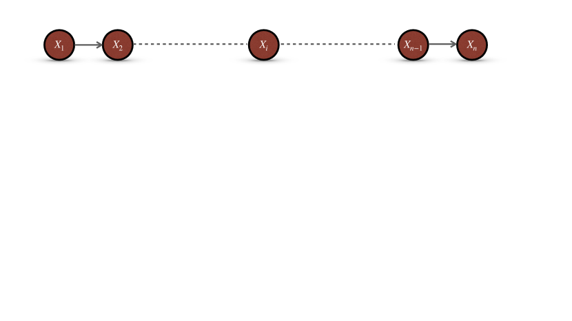
Figure 13: An inhomogeneous Markov chain consists of $X=\{X_{1},X_{2},\dots,X_{n}\}$ with $p(x)=\prod_{i=1}^{n}p(x_{i}|x_{i-1})$.




Appendix E Proof of Lemma 3.1



Since for any $Q\in\mathcal{D}_{l}^{\eta_{l}}$, we have $\pi_{j}^{Q}\equiv\pi_{j}^{P}=\pi_{j}$ and $Q_{j|\pi_{j}}\equiv P_{j|\pi_{j}}$ for all $j\neq l$, therefore, we can rewrite the bias $\mathbb{E}_{Q}\left[f(X_{k})\right]-\mathbb{E}_{P}\left[f(X_{k})\right]$ as






$$=
\int_{\mathcal{X}}f(x_{k})\prod_{i=1}^{n}Q(dx_{i}|x_{\pi_{i}^{Q}})-\int_{\mathcal{X}}f(x_{k})\prod_{i=1}^{n}P(dx_{i}|x_{\pi_{i}^{P}})$$






$$=
\int_{\mathcal{X}_{k}}\int_{\mathcal{X}_{\rho_{k}^{Q}}}f(x_{k})\prod_{i\in\rho_{k}^{Q}\cup\{k\}}Q(dx_{i}|x_{\pi_{i}^{Q}})-\int_{\mathcal{X}_{k}}\int_{\mathcal{X}_{\rho_{k}^{P}}}f(x_{k})\prod_{i\in\rho_{k}^{P}\cup\{k\}}P(dx_{i}|x_{\pi_{i}^{P}})$$






$$=
\mathbb{E}_{Q_{\{k\}}}\left[f(X_{k})\right]-\mathbb{E}_{P_{\{k\}}}\left[f(X_{k})\right]$$





If $l\notin\bar{\rho}_{k}^{P}$, we have $\pi_{i}^{Q}\equiv\pi_{i}^{P}=:\pi_{i}$ and $Q(dx_{i}|x_{\pi_{i}})\equiv P(dx_{i}|x_{\pi_{i}})$ for all $i\in\bar{\rho}_{k}$, therefore $Q_{\{k\}}\equiv P_{\{k\}}$, and thus $\mathbb{E}_{Q}\left[f(X_{k})\right]-\mathbb{E}_{P}\left[f(X_{k})\right]=0$. Based on this calculation for $Q\in\mathcal{D}_{l}^{\eta_{l}}$, we stress that our indices capture the graph structure correctly, e.g. perturbations on disconnected vertices do not affect the QoI $f=f(X_{k})$. Since $Q(dx_{j}|x_{\pi_{j}})\equiv P(dx_{j}|x_{\pi_{j}})$ for all $j\neq l$, (E) equals to



(136)

$$\;\;\;\;\;\;\;\;\;\;\;\mathbb{E}_{Q}\left[f(X_{k})\right]-\mathbb{E}_{P}\left[f(X_{k})\right]=\mathbb{E}_{Q_{\{k\}}}\left[f(X_{k})\right]-\mathbb{E}_{P_{\{k\}}}\left[f(X_{k})\right]$$




$$\qquad\;\;=\int_{\mathcal{X}_{\rho_{k}^{Q}\cup\{k\}}}f(x_{k})\prod_{i\in\rho_{k}^{Q}\cup\{k\}\setminus\rho_{l}^{Q}\cup\{l\}}Q(dx_{i}|x_{\pi_{i}^{Q}})\cdot Q(dx_{l}|x_{\pi_{l}^{Q}})\cdot\prod_{i\in\rho_{l}^{Q}}Q(dx_{i}|x_{\pi_{i}^{Q}})$$




$$\qquad\;\;\;\;-\int_{\mathcal{X}_{\rho_{k}^{P}\cup\{k\}}}f(x_{k})\prod_{i\in\bar{\rho}_{k}^{P}\setminus\rho_{l}^{P}\cup\{l\}}P(dx_{i}|x_{\pi_{i}}^{P})\cdot P(dx_{l}|x_{\pi_{l}}^{P})\cdot\prod_{i\in\rho_{l}^{P}}P(dx_{i}|x_{\pi_{i}}^{P})$$




$$\qquad\;\;=\int_{\mathcal{X}_{\rho_{k}^{P}\cup\{k\}}}f(x_{k})\prod_{i\in\bar{\rho}_{k}^{P}\setminus\rho_{l}^{P}\cup\{l\}}P(dx_{i}|x_{\pi_{i}^{P}})\cdot Q(dx_{l}|x_{\pi_{l}^{Q}})\cdot\prod_{i\in\rho_{l}^{P}}P(dx_{i}|x_{\pi_{i}^{P}})$$




$$\qquad\;\;\;\;-\int_{\mathcal{X}_{\rho_{k}^{P}\cup\{k\}}}f(x_{k})\prod_{i\in\bar{\rho}_{k}^{P}\setminus\rho_{l}^{P}\cup\{l\}}P(dx_{i}|x_{\pi_{i}^{P}})\cdot P(dx_{l}|x_{\pi_{l}^{P}})\cdot\prod_{i\in\rho_{l}^{P}}P(dx_{i}|x_{\pi_{i}^{P}})$$




$$\qquad\;\;=\int_{\mathcal{X}_{\rho_{l}^{P}}}\left[\int_{\mathcal{X}_{l}}F(x_{l},x_{\rho_{l}^{P}})Q(dx_{l}|x_{\pi_{l}^{Q}})-\int_{\mathcal{X}_{l}}F(x_{l},x_{\rho_{l}^{P}})P(dx_{l}|x_{\pi_{l}^{P}})\right]\prod_{i\in\rho_{l}}P(dx_{i}|x_{\pi_{i}^{P}})$$




$$\qquad\;\;=\mathbb{E}_{P_{\rho_{l}^{P}}}\left[\mathbb{E}_{Q_{l|\pi_{l}^{Q}}}\left[F(X_{l},X_{\rho_{l}^{P}})\right]-{\mathbb{E}_{P_{l|\pi_{l}^{P}}}\left[F(X_{l},X_{\rho_{l}^{P}})\right]}\right]$$







Appendix F KL-divergence Chain Rule for Bayesian networks


In this subsection, we discuss the KL chain rule [16] in the context of Bayesian networks as it paves the way for considering suitable ambiguity sets (different than (5)) and applying model sensitivity analysis to each component on a baseline Bayesian network. We remind that $P_{i|\pi_{i}^{P}}$ is the conditional distribution of $X_{i}$ with given parents $X_{\pi_{i}^{P}}=x_{\pi_{i}}$, i.e. $P_{i|\pi_{i}^{P}}(dx_{i})=P(dx_{i}|x_{\pi_{i}})$ and for clarity purposes and stressing the given values, we write $P_{i|X_{\pi_{i}^{P}}=x_{\pi_{i}}}(dx_{i})$
instead.



Definition F.1.


Let $P$ and $Q$ be two PGMs with densities $p$ and $q$ respectively defined as (1). For each $i\in\{1,\dots,n\}$, we define the conditional KL divergence between $Q_{i|X_{\pi_{i}^{Q}}}$ and $P_{i|X_{\pi_{i}^{P}}}$ with given $X_{\pi_{i}^{Q}}=x_{\pi_{i}^{Q}}$ and $X_{\pi_{i}^{P}}=x_{\pi_{i}^{P}}$ as



(137)

$$R(Q_{i|X_{\pi_{i}^{Q}}=x_{\pi_{i}^{Q}}}\|P_{i|X_{\pi_{i}^{P}}=x_{\pi_{i}^{P}}})=\int_{\mathcal{X}_{i}}\log\frac{Q(dx_{i}|x_{\pi_{i}^{Q}})}{P(dx_{i}|x_{\pi_{i}^{P}})}Q(dx_{i}|x_{\pi_{i}^{Q}})$$








Lemma F.2 (Chain Rule of Relative Entropy for PGMs).


For any two PGMs $P$ and $Q$ with densities $p(x)=\prod_{i=1}^{n}p(x_{i}|x_{\pi_{i}^{P}})$ and $q(x)=\prod_{i=1}^{n}q(x_{i}|x_{\pi_{i}^{Q}})$, the KL divergence can be expressed as:



(138)

$$R(Q\|P)=\sum_{i=1}^{n}\mathbb{E}_{Q_{\pi_{i}^{Q}\cup\pi_{i}^{P}}}\left[R(Q_{i|X_{\pi_{i}^{Q}}}\|P_{i|X_{\pi_{i}^{P}}})\right]$$



where $R(Q_{i|X_{\pi_{i}^{Q}}}\|P_{i|X_{\pi_{i}^{P}}})$ is the conditional KL divergence given in Definition F.1 and $\mathbb{E}_{Q_{\pi_{i}^{Q}\cup\pi_{i}^{P}}}$ is the expectation with respect to $Q_{A}$ defined in Section 2 with $A=\pi_{i}^{Q}\cup\pi_{i}^{P}$.





Proof F.3.







$$\;\;\;\;\;\;\;\;\;\;\;R(Q\|P)
=
\int_{\mathcal{X}}\sum_{i=1}^{n}\log\frac{Q(dx_{i}|x_{\pi_{i}^{Q}})}{P(dx_{i}|x_{\pi_{i}^{P}})}\prod_{j=1}^{n}Q(dx_{j}|x_{\pi_{j}^{Q}})$$







$$=
\sum_{i=1}^{n}\int_{\mathcal{X}_{\rho_{i}^{P}\cup\rho_{i}^{Q}}}\int_{\mathcal{X}_{i}}\log\frac{Q(dx_{i}|x_{\pi_{i}^{Q}})}{P(dx_{i}|x_{\pi_{i}^{P}})}Q(dx_{i}|x_{\pi_{i}^{Q}})\prod_{j\in\{\rho_{i}^{Q}\cup\rho_{i}^{P}\}}Q(dx_{j}|x_{\pi_{j}^{Q}})$$






$$=
\sum_{i=1}^{n}\mathbb{E}_{Q_{\pi_{i}^{Q}\cup\pi_{i}^{P}}}\left[R(Q_{i|X_{\pi_{i}^{Q}}}\|P_{i|X_{\pi_{i}^{P}}})\right]$$











Appendix G Schematic for Model Sensitivity Indices


This schematic refers to the main theorems of Section 3.





Appendix H Data-informed stress tests for Gaussian Bayesian networks


In this section, we explain with detail Data-informed stress tests analysis when the baseline model $P$ is a Gaussian Bayesian network. Let $P$ be a Gaussian Bayesian network with conditional probability densities $p(x_{i}|x_{\pi_{i}})$ satisfying $p(x_{i}|x_{\pi_{i}})=\mathcal{N}(\beta_{i0}+\beta_{i}^{T}x_{\pi_{i}},\sigma_{i}^{2})$ for some $\beta_{i0}$, $\beta_{i}$, and $\sigma_{i}^{2}$, i.e. $P_{i|\pi_{i}}$ is the conditional distribution of $X_{i}=\beta_{i0}+\beta_{i}^{T}X_{\pi_{i}}+\epsilon_{i}$. The random variable $\epsilon_{i}$ has density $p_{\epsilon_{i}}(x)=\mathcal{N}(0,\sigma_{i}^{2})$ and comes from fitting data with Maximum-Likelihood-Estimation. Let us consider alternative models to $P$ such as



(140)

$$Q_{i|\pi_{i}}:\quad X_{i}=\beta_{i0}+\beta_{i}^{T}X_{\pi_{i}}+\tilde{\epsilon}_{i}$$



where $\tilde{\epsilon}_{i}$ follows another approximate distribution of the data with density $q_{\tilde{\epsilon}_{i}}(x)$. For instance, we can consider $Q_{\tilde{\epsilon}_{i}}$ with density $q_{\tilde{\epsilon}_{i}}$ as the histogram, that is



(141)

$$q_{\tilde{\epsilon}_{i}}^{hist}(x)=\sum_{k=1}^{m}\frac{\nu_{k}}{nh}I(x\in B_{k})\,,$$



where ${B_{1},\dots,B_{m}}$ are the histogram bins, $h$ is the bin width, $n$ is the number of observations and $\nu_{k}$ is the number of observations in $B_{k}$. Alternatively, we can consider the model $Q_{\tilde{\epsilon}_{i}}$ given by a KDE viewed here as a high resolution but smooth approximation of the histogram, namely



(142)

$$q_{\tilde{\epsilon}_{i}}^{KDE}(x)=\sum_{k=1}^{n}\frac{1}{nh}K(\frac{x-x_{i}}{h})\,,$$



where $K(\cdot)$ is the normal kernel smoothing function with bin width $h$, $(x_{1},\dots,x_{n})$ are the samples of $\epsilon_{i}$. Other KDE kernels can be considered here (see [72]) or any other probabilistic representations of the data in the histogram. Then, based on the following computation:Therefore, for given $x_{\pi_{i}}$, we have




(143)

$$\eta_{i}^{\pi_{i}}
=
\int\log\frac{q(x_{i}|x_{\pi_{i}})}{p(x_{i}|x_{\pi_{i}})}q(x_{i}|x_{\pi_{i}})dx_{i}$$







$$=
\int\log\frac{q(x_{i}-\beta_{i0}-\beta_{i}^{T}x_{\pi_{i}}|x_{\pi_{i}})}{p(x_{i}-\beta_{i0}-\beta_{i}^{T}x_{\pi_{i}}|x_{\pi_{i}})}q(x_{i}-\beta_{i0}-\beta_{i}^{T}x_{\pi_{i}}|x_{\pi_{i}})dx_{i}$$






$$=
\int\log\frac{q_{\tilde{\epsilon}_{i}}(x)}{p_{\epsilon_{i}}(x)}q_{\tilde{\epsilon}_{i}}(x)dx\,,$$





Based on the above computation, $\eta_{i}^{\pi_{i}}$ is independent of $\pi_{i}$ and hence $\eta_{i}^{\pi_{i}}\equiv\eta_{i}$.




Appendix I Model sensitivity indices for the ORR Bayesian network


Table 1: Outcomes of MLE for the parameters involved in (80)-(82) for the ORR Bayesian network in Section 7.



     $\beta_{y_{1},0}$ = 0.0595
     $\beta_{e0,0}$, $\beta_{ei,0}$ = 0




     $\sigma_{e0}^{2}$ = 0.0329
     $\sigma_{ei}^{2}$ = 0.0065


     $\beta_{y_{2},0}$ = 1.8231
     $\beta_{d0,0}$ = -0.0754


     $\beta_{di,0}$ = -0.0222
     $\sigma_{di}^{2}$ = 0.0354


     $\beta_{y_{1},x_{0}}$ = 0.5111
     $\sigma_{d0}^{2}$ = 0.1032


     $\beta_{s1,0}$ = -0.2967
     $\sigma_{s1}^{2}$ = 0.0046


     $\beta_{y_{2},x_{0}}$ = -0.5564
     $\beta_{s0,0}$ = 0.0067


     $\beta_{s2,0}$ = -0.1209
     $\sigma_{s2}^{2}$ = 0.0054


     $\beta_{ci,0}$ = 0
     $\sigma_{s0}^{2}$ = 0.0010


     $\sigma_{c1}^{2}$ = 0.0347
     $\sigma_{c2}^{2}$ = 0.0204






I.1 Calculation of model sensitivity indices


We remind that the optimal oxygen binding energy is defined as




$$x_{O^{*}}^{P}=\mathrm{argmax}_{x_{0}}\left[\min\{\mathbb{E}_{P}\left[y_{1}|x_{0}\right],\mathbb{E}_{P}\left[y_{2}|x_{0}\right]\}\right]$$



We compute $\mathbb{E}_{P}\left[y_{i}|x_{0}\right]$ for $i=1,2$ by using (79) and (82) as follows





$$\mathbb{E}_{P}\left[y_{i}|x_{0}\right]
=
\beta_{y_{i},0}+\beta_{y_{i},x}(x_{0}+\beta_{s0,0}+\beta_{e0,0}+\beta_{d0,0})$$








$$\qquad+\beta_{ci,0}+\beta_{si,0}+\beta_{ei,0}+\beta_{di,0}$$




Then



(144)

$$x_{O^{*}}^{P}=\frac{\beta_{y_{2},0}+\bar{\beta}_{2}-\beta_{y_{1},0}-\bar{\beta}_{1}}{\beta_{y_{1},x}-\beta_{y_{2},x}}$$



where



(145)

$$\bar{\beta}_{i}=\beta_{y_{i},x}(\beta_{s0,0}+\beta_{e0,0}+\beta_{d0,0})+\beta_{ci,0}+\beta_{si,0}+\beta_{ei,0}+\beta_{di,0}$$



It is a straightforward calculation that for $i=1,2$ and $l=e0,d0,s0,e1,d1,s1,c1,e2,d2,s2$ and $c2$.




$$\beta_{y_{i},0}+\bar{\beta}_{i}=\mathbb{E}_{P_{\omega_{l}}}\left[F_{l,i}\right],\qquad\textrm{ for any $i$ and $l$}$$



where $F_{l,i}=\mathbb{E}_{P_{y_{i}|\omega_{l}}}\left[y_{i}|x_{0}\right]$ and $p(y_{i}|\omega_{l},x_{0})=\mathcal{N}(\tilde{\beta}_{y_{i},0}+\tilde{\beta}_{y_{i},\omega_{l}}\omega_{l},\tilde{\sigma}_{y_{i}}^{2})$. Hence (144) equals to




$$x_{O^{*}}^{P}=\frac{\mathbb{E}_{P_{\omega_{l}}}\left[F_{l,2}\right]-\mathbb{E}_{P_{\omega_{l}}}\left[F_{l,1}\right]}{\beta_{y_{1},x}-\beta_{y_{2},x}}$$



Note that since we compute the model sensitivity indices over $\mathcal{D}_{l,P}^{\eta_{l}}$ for any $l\in\{e0,d0,s0,e1,d1,s1,c1,e2,d2,s2\}$, the alternative Bayesian networks $Q$ have the same structure given by (79), same CPDs as the Bayesian network $P$ except from the CPD of $\omega_{l}$. Let us denote its conditional distribution by $Q_{\omega_{l}}$(since $\rho_{\omega_{l}}=\pi_{\omega_{l}}=\emptyset$) and its CPD by $q_{\omega_{l}}$. Then,



(146)

$$x_{O^{*}}^{Q}-x_{O^{*}}^{P}=\frac{\mathbb{E}_{Q_{\omega_{l}}}\left[F_{l,2}\right]-\mathbb{E}_{P_{\omega_{l}}}\left[F_{l,2}\right]-(\mathbb{E}_{Q_{\omega_{l}}}\left[F_{l,2}\right]-\mathbb{E}_{P_{\omega_{l}}}\left[F_{l,1}\right])}{\beta_{y_{1},x}-\beta_{y_{2},x}}$$



which further gives us




$$\frac{I^{\mp}(y_{2},P;\mathcal{D}^{\eta_{l}}_{l,P})-I^{\pm}(y_{1},P;\mathcal{D}^{\eta_{l}}_{l,P})}{\beta_{y_{1},x}-\beta_{y_{2},x}}\leq x_{O^{*}}^{Q}-x_{O^{*}}^{P}\leq\frac{I^{\pm}(y_{2},P;\mathcal{D}^{\eta_{l}}_{l,P})-I^{\mp}(y_{1},P;\mathcal{D}^{\eta_{l}}_{l,P})}{\beta_{y_{1},x}-\beta_{y_{2},x}}$$



In the above inequality, by combining Corollary 3.8 and Table 2 we get (85) and (86).


Table 2: The values of $\tilde{\beta}_{y_{i},\omega_{l}}$ involved in $p(y_{i}|\omega_{l},x_{0})=\mathcal{N}(\tilde{\beta}_{y_{i},0}+\tilde{\beta}_{y_{i},\omega_{l}}\omega_{l},\tilde{\sigma}_{y_{i}}^{2})$. They are used to evaluate the model sensitivity indices $I^{\pm}(y_{i},P;\mathcal{D}^{\eta_{l}}_{l,P})$, $i=1,2$ provided by Corollary 3.8.




$\omega_{l}=\omega_{e0},\omega_{d0},\omega_{s0}$
$\omega_{l}=\omega_{e1},\omega_{d1},\omega_{s1},\omega_{c1}$
$\omega_{l}=\omega_{e2},\omega_{d2},\omega_{s2},\omega_{c2}$




$f=y_{1}$
$\tilde{\beta}_{y_{1},\omega_{l}}=\beta_{y_{1},x}$
$\tilde{\beta}_{y_{1},\omega_{l}}=1$
$\tilde{\beta}_{y_{1},\omega_{l}}=0$


$f=y_{2}$
$\tilde{\beta}_{y_{2},\omega_{l}}=\beta_{y_{2},x}$
$\tilde{\beta}_{y_{2},\omega_{l}}=0$
$\tilde{\beta}_{y_{2},\omega_{l}}=1$







I.2 Propagation of model uncertainties to the QoIs


We note the discrepancies in the propagation of model misspecification to the QoI between different Bayesian network components, as demonstrated in Figure 9. In particular, in Figure 9 (Left) the same uncertainty (described by model misspecification $\eta_{l}$) is applied on all ORR Bayesian network vertices, however not all propagate and affect the same the QoI: see Figure 15 for examples of propagation ($22\%$) and non-propagation ($5\%$ and $0\%$) of model misspecification to the QoI.


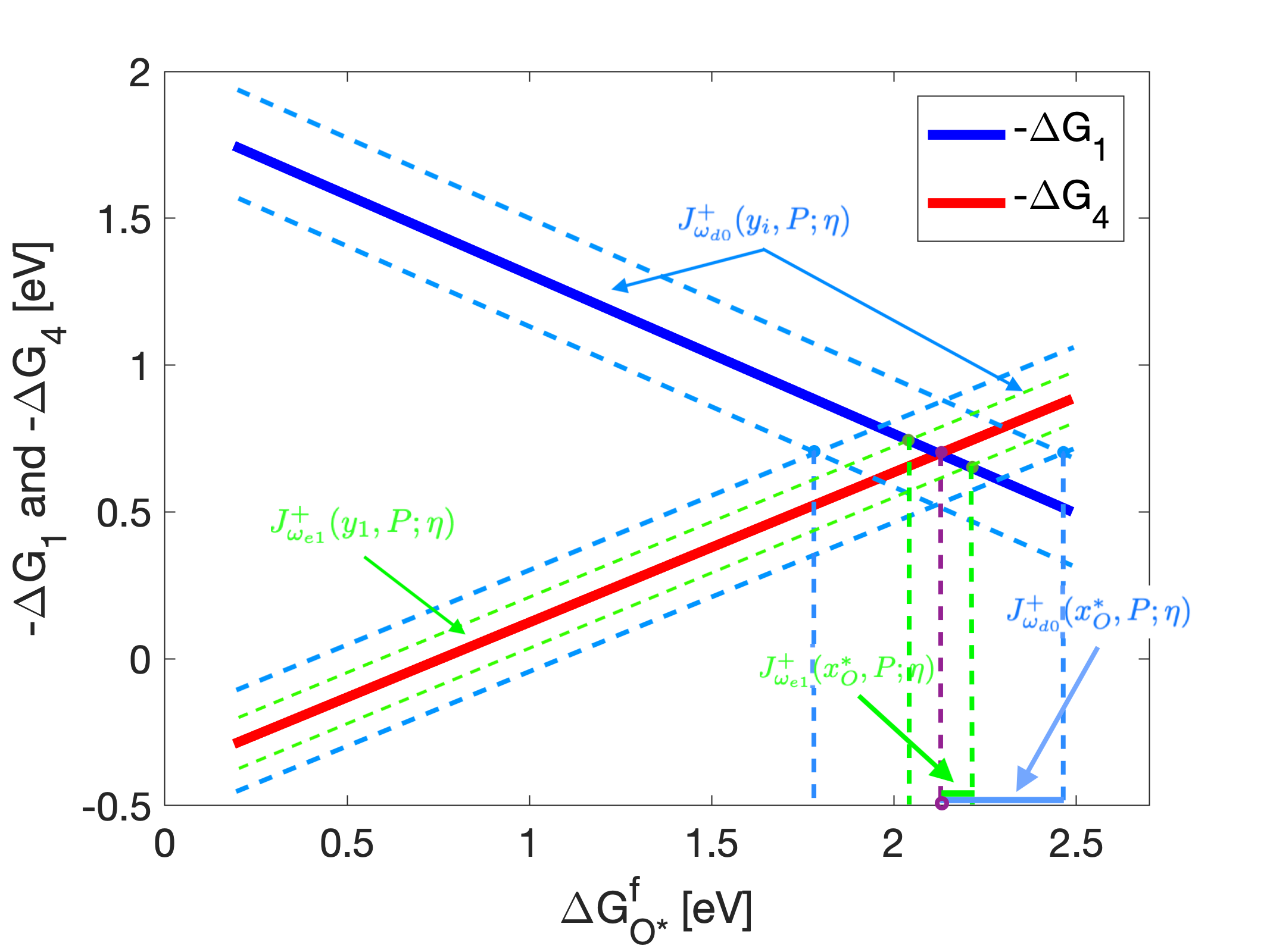
Figure 15: Propagation vs. Non-propagation
of model misspecification of the Bayesian network vertices $\omega_{d0}$ and $\omega_{e1}$ respectively, to the predictions of the QoI $x_{O^{\ast}}^{P}$; model misspecification is set to $\eta=1$ for both Bayesian network vertices. First, note that $I^{+}(y_{2},P;\mathcal{D}^{\eta}_{\omega_{e1}})=0$ i.e., the model misspecification of $\omega_{e1}$ only affects the prediction of $y_{1}$, but not $y_{2}$, see Figure 8; therefore the uncertainty of $\omega_{e1}$ only propagates to $x_{O^{\ast}}^{P}$ through $y_{1}$, while $I^{+}(y_{1},P;\mathcal{D}^{\eta}_{\omega_{e1}})$ is small since $\omega_{e1}$ has a lower variance which is associated with more informative available data. Thus, it results in a small corresponding uncertainty in $x_{O^{\ast}}^{P}$. Meanwhile, the uncertainty of $\omega_{d0}$ propagates to $x_{O^{\ast}}^{P}$ through both $y_{1}$ and $y_{2}$, (i.e., the model misspecification of $\omega_{d0}$ affects both the predictions of $y_{1}$ and $y_{2}$), and $I^{+}(y_{i},P;\mathcal{D}^{\eta}_{\omega_{d0}})$ is larger since $\omega_{d0}$ has a higher variance (due to insufficient informative data available). Therefore we have a larger corresponding uncertainty in $x_{O^{\ast}}^{P}$ predictions, as shown in the figure.

References

[1]
Amina Adadi and Mohammed Berrada.
Peeking inside the black-box: A survey on explainable artificial
intelligence (xai).
IEEE Access, 6:52138–52160, 2018.
[2]
Olivier Antoine, Yann Bultel, and Robert Durand.
Oxygen reduction reaction kinetics and mechanism on platinum
nanoparticles inside nafion®.
Journal of Electroanalytical Chemistry, 499(1):85–94, 2001.
[3]
Dominik Aronsky and Peter J Haug.
Diagnosing community-acquired pneumonia with a bayesian network.
In Proceedings of the AMIA Symposium, page 632. American
Medical Informatics Association, 1998.
[4]
Mohamed Ishmael Belghazi, Aristide Baratin, Sai Rajeshwar, Sherjil Ozair,
Yoshua Bengio, Aaron Courville, and Devon Hjelm.
Mutual information neural estimation.
In Jennifer Dy and Andreas Krause, editors, Proceedings of the
35th International Conference on Machine Learning, volume 80 of Proceedings of Machine Learning Research, pages 531–540. PMLR, 10–15 Jul
2018.
[5]
Panagiota Birmpa and Markos A. Katsoulakis.
Uncertainty quantification for markov random fields.
arXiv preprint, arXiv: 2009.00038, 2020.
[6]
Jeremiah Birrell, Paul Dupuis, Markos A. Katsoulakis, Yannis Pantazis,
and Luc Rey-Bellet.
-Divergences: Interpolating between -Divergences and
Integral Probability Metrics.
arXiv e-prints, page arXiv:2011.05953, November 2020.
[7]
Jeremiah Birrell, Paul Dupuis, Markos A. Katsoulakis, Luc Rey-Bellet, and Jie
Wang.
Variational representations and neural network estimation of rényi
divergences.
arXiv preprint, arXiv:2007.03814, 2021.
[8]
Jeremiah Birrell, Markos Katsoulakis, and Luc Rey-Bellet.
Robustness of Dynamical Quantities of Interest via Goal-Oriented
Information Theory.
arXiv e-prints, page arXiv:1906.09282, Jun 2019.
[9]
Jeremiah Birrell and Luc Rey-Bellet.
Uncertainty quantification for markov processes via variational
principles and functional inequalities.
SIAM/ASA Journal on Uncertainty Quantification, 8(2):539–572,
2020.
[10]
Christopher M. Bishop.
Pattern Recognition and Machine Learning (Information Science
and Statistics).
Springer-Verlag New York, Inc., Secaucus, NJ, USA, 2006.
[11]
Jose Blanchet, Henry Lam, Qihe Tang, and Zhongyi Yuan.
Robust actuarial risk analysis.
North American Actuarial Journal, 23(1):33–63, 2019.
[12]
Jose Blanchet and Karthyek Murthy.
Quantifying distributional model risk via optimal transport.
Mathematics of Operations Research, 44(2):565–600, 2019.
[13]
C. Burges, Ted Hart, Zi Yang, Silviu Cucerzan, Ryen W. White, A. Pastusiak, and
J. Lewis.
A base camp for scaling ai.
arXiv: 1612.07896, 2016.
[14]
Federico Calle-Vallejo, Jakub Tymoczko, Viktor Colic, Quang Huy Vu, Marcus D
Pohl, Karina Morgenstern, David Loffreda, Philippe Sautet, Wolfgang
Schuhmann, and Aliaksandr S Bandarenka.
Finding optimal surface sites on heterogeneous catalysts by counting
nearest neighbors.
Science, 350(6257):185–189, 2015.
[15]
Kamaljit Chowdhary and Paul Dupuis.
Distinguishing and integrating aleatoric and epistemic variation in
uncertainty quantification.
ESAIM: Mathematical Modelling and Numerical Analysis,
47(03):635–662, 2013.
[16]
Thomas M Cover and Joy A Thomas.
Elements of information theory.
John Wiley & Sons, 2012.
[17]
Erick Delage and Yinyu Ye.
Distributionally robust optimization under moment uncertainty with
application to data-driven problems.
Operations Research, 58(3):595–612, 2010.
[18]
Mucong Ding, C. Daskalakis, and S. Feizi.
Gans with conditional independence graphs: On subadditivity of
probability divergences.
In AISTATS, 2021.
[19]
Finale Doshi-Velez and Been Kim.
Towards a rigorous science of interpretable machine learning.
arXiv: 1702.08608, 2017.
[20]
Paul Dupuis and Richard S Ellis.
A weak convergence approach to the theory of large deviations,
volume 902.
John Wiley & Sons, 2011.
[21]
Paul Dupuis, Markos A Katsoulakis, Yannis Pantazis, and Petr Plechác.
Path-space information bounds for uncertainty quantification and
sensitivity analysis of stochastic dynamics.
SIAM/ASA Journal on Uncertainty Quantification, 4(1):80–111,
2016.
[22]
Paul Dupuis, Markos A Katsoulakis, Yannis Pantazis, and Luc Rey-Bellet.
Sensitivity analysis for rare events based on rényi divergence.
arXiv preprint arXiv:1805.06917, 2018.
[23]
Paul Dupuis and Yixiang Mao.
Formulation and properties of a divergence used to compare
probability measures without absolute continuity.
arXiv preprint, arXiv:1911.07422, 2019.
[24]
Jinchao Feng, Joshua Lansford, Alexander Mironenko, Davood Babaei Pourkargar,
Dionisios G. Vlachos, and Markos A. Katsoulakis.
Non-parametric correlative uncertainty quantification and sensitivity
analysis: Application to a langmuir bimolecular adsorption model.
AIP Advances, 8(3):035021, 2018.
[25]
Jinchao Feng, Joshua Lansford, Alexander Mironenko, Davood Babaei Pourkargar,
Dionisios G Vlachos, and Markos A Katsoulakis.
Non-parametric correlative uncertainty quantification and sensitivity
analysis: Application to a langmuir bimolecular adsorption model.
AIP Advances, 8(3):035021, 2018.
[26]
Jinchao Feng, Joshua L. Lansford, Markos A. Katsoulakis, and Dionisios G.
Vlachos.
Explainable and trustworthy artificial intelligence for correctable
modeling in chemical sciences.
Science Advances, 6(42), 2020.
[27]
Nir Friedman, Michal Linial, Iftach Nachman, and Dana Pe’er.
Using bayesian networks to analyze expression data.
Journal of computational biology, 7(3-4):601–620, 2000.
[28]
Robert Fung and Brendan Del Favero.
Applying bayesian networks to information retrieval.
Communications of the ACM, 38(3):42–ff, 1995.
[29]
Rui Gao and Anton J. Kleywegt.
Distributionally Robust Stochastic Optimization with Wasserstein
Distance.
arXiv e-prints, page arXiv:1604.02199, Apr 2016.
[30]
Aude Genevay, Gabriel Peyré, and Marco Cuturi.
GAN and VAE from an Optimal Transport Point of View.
arXiv e-prints, page arXiv:1706.01807, June 2017.
[32]
Pierre Glaser, Michael Arbel, and Arthur Gretton.
KALE Flow: A Relaxed KL Gradient Flow for Probabilities with
Disjoint Support.
arXiv e-prints, page arXiv:2106.08929, June 2021.
[33]
Joel Goh and Melvyn Sim.
Distributionally robust optimization and its tractable
approximations.
Operations Research, 58(4-part-1):902–917, 2010.
[34]
Miguel A Gómez-Villegas, Paloma Maín, and Rosario Susi.
Sensitivity analysis in gaussian bayesian networks using a divergence
measure.
Communications in Statistics—Theory and Methods,
36(3):523–539, 2007.
[35]
Miguel A Gómez-Villegas, Paloma Main, and Rosario Susi.
The effect of block parameter perturbations in gaussian bayesian
networks: Sensitivity and robustness.
Information Sciences, 222:439–458, 2013.
[36]
Miguel Ángel Gómez-Villegas, Paloma Main, Hilario Navarro, and Rosario
Susi.
Evaluating the difference between graph structures in gaussian
bayesian networks.
Expert Systems with Applications, 38(10):12409–12414, 2011.
[37]
Konstantinos Gourgoulias, M. Katsoulakis, L. Rey-Bellet, and J. Wang.
How biased is your model? concentration inequalities, information and
model bias.
IEEE Transactions on Information Theory, 66:3079–3097, 2020.
[38]
David Gunning and David Aha.
Darpa’s explainable artificial intelligence (xai) program.
AI Magazine, 40(2):44–58, Jun. 2019.
[39]
E. Hall and M. Katsoulakis.
Robust information divergences for model-form uncertainty arising
from sparse data in random pde.
SIAM/ASA J. Uncertain. Quantification, 6:1364–1394, 2018.
[40]
Eric J. Hall, SÞren Taverniers, Markos A. Katsoulakis, and Daniel M.
Tartakovsky.
Ginns: Graph-informed neural networks for multiscale physics.
Journal of Computational Physics, 433:110192, 2021.
[41]
Lars Peter Hansen and Thomas J. Sargent.
Robustness.
Princeton University Press, stu - student edition edition, 2008.
[42]
David Heckerman, Eric Horvitz, and Bharat N Nathwani.
Toward normative expert systems part i.
Methods of information in medicine, 31, 2016.
[43]
Adam Holewinski and Suljo Linic.
Elementary mechanisms in electrocatalysis: revisiting the orr tafel
slope.
Journal of The Electrochemical Society, 159(11):H864, 2012.
[45]
Kirthevasan Kandasamy, Akshay Krishnamurthy, Barnabÿs Póczos, Larry
Wasserman, and James M. Robins.
Nonparametric von mises estimators for entropies, divergences and
mutual informations.
In Proceedings of the 28th International Conference on Neural
Information Processing Systems - Volume 1, NIPS’15, page 397–405,
Cambridge, MA, USA, 2015. MIT Press.
[46]
Michael G. Kapteyn, Jacob V. R. Pretorius, and Karen E. Willcox.
A Probabilistic Graphical Model Foundation for Enabling Predictive
Digital Twins at Scale.
arXiv e-prints, page arXiv:2012.05841, December 2020.
[47]
Markos A Katsoulakis, Luc Rey-Bellet, and Jie Wang.
Scalable information inequalities for uncertainty quantification.
Journal of Computational Physics, 336:513–545, 2017.
[48]
Daphne Koller and Nir Friedman.