Topologically protected two-fluid edge states

Abstract

Edge states reveal the nontrivial topology of energy band in the bulk. As localized states at boundaries, many-body edge states may obey a special symmetry that is broken in the bulk. When local particle-particle interaction is induced, they may support a particular property. We consider an extended two-dimensional Su-Schrieffer-Heeger Hubbard model and examine the appearance of $\eta$-pairing states, which are excited eigenstates related to superconductivity. In the absence of Hubbard interaction, the energy band is characterized by topologically invariant polarization in association with edge states. In the presence of on-site Hubbard interaction, $\eta$-pairing edge states appear in the topologically nontrivial phase, resulting in the condensation of pairs at the boundary. In addition, as Hamiltonian eigenstates, the edge states contain paired fermions and unpaired fermions. Neither affects the other; they act as two-fluid states. From numerical simulations of many-body scattering processes, a clear manifestation and experimental detection scheme of topologically protected two-fluid edge states are provided.

I Introduction

Topology in matter permits the existence of edge states, which have a strong immunity to distortions of the underlying architecture. Although they are believed to be inherited from the topology of the bulk, these edge states present some properties only around the boundary and are forbidden in the bulk. Topological insulator in condensed matter physics is a well-known example of this phenomenon. Although such a system is an insulator in the bulk, it permits electron conductance along the edges, resulting in quantized Hall conductance [1, 2, 3, 4]. In general, the strong interaction between fermions can affect the topology of a fermion system and break the bulk-boundary correspondence (BBC) [5]. Nevertheless, recent work [6] shows that quantum spin system also exhibits BBC even in a thermal state. This indicates that although the BBC reveals a nontrivial topology of the energy band, it has a particular feature in the presence of interaction.

Beyond the realm of the well-known topological insulator, recent studies on the twisted bilayer graphene (TBG) show that at a series of magic twist angles, the moiré pattern yields the flat low-energy bands that promise strong electronic correlations [7, 8, 9]. The interplay of lattice geometry and many-body interactions induces exotic quantum states including superconducting [10, 11] and correlated insulating [12] behaviors, which have been achieved in experiments [13, 14]. An interesting question is whether such exotic quantum states exist in a topological system, where the energy band of edge states plays the same role as the moiré flat band, in the presence of strong electronic correlations. The $\eta$ pairing proposed by Yang [15] is a promising mechanism to address this problem. In the absence of Hubbard interaction $U$, an $\eta$ pair has zero energy in a bipartite lattice, thus the flat band appears when considering multiple $\eta$ pairs formed by electrons with momentums $\mathbf{k}$ and $\boldsymbol{\pi}-\mathbf{k}$ [15]. There are two common grounds between the flat bands of TBG and that of many-body edge states: They are formed by breaking the translational symmetry and have the potential to enhance electronic correlations. Importantly, such paired states become long lived in the presence of strong Hubbard repulsion [16, 17, 18, 19]. In addition, recent theoretical works [20, 21] suggest that the $\eta$-pairing states can be induced by pulse irradiation or heating. On the other hand, as a phenomenological theory, the two-fluid model was proposed several decades ago to explain the behavior of superfluid helium [22, 23] and a conventional superconductor [24]. It postulates that a superconductor possesses two parallel channels, one superconducting and one normal. Although it is a useful tool, so far two-fluid states have yet to be investigated in the framework of quantum mechanics, appearing as a many-body Hamiltonian eigenstate. For instance, even the usual BCS wave function [25] is not an eigenstate of a Hamiltonian system with a local potential energy.

In this paper, we consider an extended two-dimensional (2D) Su-Schrieffer-Heeger (SSH) [26] model with on-site Hubbard interaction $U$. Specifically, we examine the appearance of $\eta$-pairing edge states [see Fig. 1(a)]. In the absence of Hubbard interaction, the energy band is characterized by topologically invariant polarization in association with edge states. When $U$ switches on, the bulk states do not support the formation of $\eta$ pairs, which appear only at the edge and possess an off-diagonal long-range order (ODLRO) [27] in the topologically nontrivial phase. We further propose a concept of topologically protected two-fluid edge states. As many-body eigenstates of a 2D SSH Hubbard model, the two-fluid edge states contain two components: $\eta$-pairing fermions and unpaired fermions, which do not affect each other. The signature of the two-fluid edge states is observable in the dynamic behavior of resonant transmission. Based on the non-Hermitian quantum mechanics [28, 29, 30, 31, 32], we also develop a method to resolve the scattering problem involving multiple interacting fermions.

The remainder of this paper is organized as follows. In Sec. II, we introduce the concept of two-fluid states by a Hubbard model. In Sec. III, we demonstrate the existence of topological $\eta$-paring edge states in an extended 2D SSH Hubbard model, which also supports two-fluid edge states and the properties are studied in Sec. IV through dynamics of resonant transmission. In Sec. V, we summarize our results.

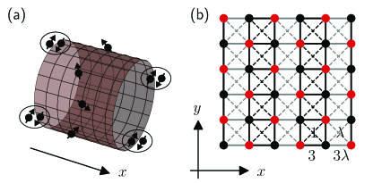
Figure 1: (a) Schematic of the lattice with cylindrical boundary condition. The lattice supports $\eta$-pairing edge states, whereas the bulk states are unpaired fermions. (b) Details of the lattice, which is an extended 2D SSH Hubbard model depicted by the Hamiltonian in Eq. (9). The black and red dots represent sublattices A and B, respectively. The solid and dashed lines represent the nearest-neighbor and next-nearest-neighbor hopping, respectively.

II Model and two-fluid states

We begin with the Hamiltonian model of a general form and a brief summary of related results. The Hamiltonian is in the following form

$$H=H_{0}+H_{\mathrm{intra}},$$ (1)

on two sublattices $\mathrm{A}$ and $\mathrm{B}$. Here $H_{0}$ is the Hamiltonian of a simple Hubbard model with bipartite lattice symmetry

$$H_{0}=\sum_{\mathbf{r}\in\mathrm{A},\mathbf{r}^{\prime}\in\mathrm{B}}\sum_{\sigma=\uparrow,\downarrow}t_{\mathbf{rr}^{\prime}}c_{\mathbf{r},\sigma}^{\dagger}c_{\mathbf{r}^{\prime},\sigma}+\text{{H.c.}}+U\sum_{\mathbf{r}\in\mathrm{A}\cup\mathrm{B}}n_{\mathbf{r},\uparrow}n_{\mathbf{r},\downarrow},$$ (2)

where the operator $c_{\mathbf{r},\sigma}$ ($c_{\mathbf{r},\sigma}^{\dagger}$) is the usual annihilation (creation) operator of a fermion with spin $\sigma\in\left\{\uparrow,\downarrow\right\}$ at site $\mathbf{r}$, and $n_{\mathbf{r},\sigma}=c_{\mathbf{r},\sigma}^{\dagger}c_{\mathbf{r},\sigma}$ is the number operator for a particle of spin $\sigma$ on site $\mathbf{r}$. As many previous studies [16, 17, 18, 19, 20, 21], here the interaction is purely on-site. Nevertheless, the weak nearest-neighbor interaction does not break the paired states [33] considered below. Unlike almost all studies on the $\eta$-pairing states, we consider an extra term $H_{\mathrm{intra}}$, representing the intrasublattice hopping. This term breaks the bipartite symmetry of $H_{0}$.

We first review well-established model properties of $H_{0}$ that are crucial to our conclusion (see Appendix A for more details). First, $H_{0}$ possesses SU(2) symmetry characterized by the generators $s^{+}=\left(s^{-}\right)^{\dagger}=\sum_{\mathbf{r}}s_{\mathbf{r}}^{+}$ and $s^{z}=\sum_{\mathbf{r}}s_{\mathbf{r}}^{z}$, where $s_{\mathbf{r}}^{+}=c_{\mathbf{r},\uparrow}^{\dagger}c_{\mathbf{r},\downarrow}$ and $s_{\mathbf{r}}^{z}=\left(n_{\mathbf{r},\uparrow}-n_{\mathbf{r},\downarrow}\right)/2$. Second, one can define the following operators

$$\eta^{+}=\left(\eta^{-}\right)^{\dagger}=\sum_{\mathbf{r}}\eta_{\mathbf{r}}^{+},\quad\eta^{z}=\sum_{\mathbf{r}}\eta_{\mathbf{r}}^{z},$$ (3)

with $\eta_{\mathbf{r}}^{+}=c_{\mathbf{r},\uparrow}^{\dagger}c_{\mathbf{r},\downarrow}^{{\dagger}}$ ($-c_{\mathbf{r},\uparrow}^{\dagger}c_{\mathbf{r},\downarrow}^{{\dagger}}$) for $\mathbf{r}\in A$ ($\mathbf{r}\in B$), and $\eta_{\mathbf{r}}^{z}=\left(n_{\mathbf{r},\uparrow}+n_{\mathbf{r},\downarrow}-1\right)/2$, satisfying commutation relation $[\eta_{\mathbf{r}}^{+},$ $\eta_{\mathbf{r}}^{-}]=2\eta_{\mathbf{r}}^{z}$ and $[\eta_{\mathbf{r}}^{z},$ $\eta_{\mathbf{r}}^{\pm}]=\pm\eta_{\mathbf{r}}^{\pm}$. Straightforward algebra shows that

$$\left[H_{0}-U\eta^{z},\eta^{\pm}\right]=\left[H_{0},\eta^{z}\right]=0,$$ (4)

which is guaranteed by the bipartite lattice symmetry. These two properties allow the construction of two types of eigenstates of $H_{0}$: ferromagnetic (FM) and antiferromagnetic (AFM).

An $m$-fermion FM eigenstate with energy $\sum_{\left\{\mathbf{k}\right\}}^{m}\varepsilon_{\mathbf{k}}$ can be expressed as follows:

$$\left|\psi_{\mathrm{FM}}(m,l)\right\rangle=\left(s^{-}\right)^{\left(m-l\right)/2}\prod_{\left\{\mathbf{k}\right\}}^{m}c_{\mathbf{k},\uparrow}^{\dagger}\left|\mathrm{Vac}\right\rangle,$$ (5)

where $\left|\mathrm{Vac}\right\rangle$ is the vacuum state of the fermion $c_{\mathbf{r},\sigma}$, and $c_{\mathbf{k},\uparrow}^{\dagger}$ is the eigenmode of $H_{0}$ with $U=0$ —that is, $[c_{\mathbf{k},\sigma}^{\dagger},H_{0}(U=0)]=-\varepsilon_{\mathbf{k}}c_{\mathbf{k},\sigma}^{\dagger}$. Eigenstate $\left|\psi_{\mathrm{FM}}(m,l)\right\rangle$ is a saturated FM state, given that it is also an eigenstate of $s^{2}$ and $s^{z}$, with eigenvalues $m\left(m/2+1\right)/2$ and $l/2,$ respectively.

An $n$-pair AFM eigenstate can be expressed as

$$\left|\psi_{\mathrm{AFM}}(n)\right\rangle=\left(\eta^{+}\right)^{n}\left|\mathrm{Vac}\right\rangle,$$ (6)

which obeys $H_{0}\left|\psi_{\mathrm{AFM}}(n)\right\rangle=nU\left|\psi_{\mathrm{AFM}}(n)\right\rangle$ and $s^{2}\left|\psi_{\mathrm{AFM}}(n)\right\rangle=0$. Obviously, an $\eta$-pairing state is spin singlet. Unlike all other spin singlet states, an AFM $\eta$-pairing eigenstate is independent of the detailed structure of the bipartite lattice, regardless of whether it contains short-, long-, or even infinite-range hopping terms. This feature is characterized by a correlator related to the off-diagonal element of the reduced density matrix of the system [27, 15].

Importantly, there is a mixture of two types of states, referred to as two-fluid state

$$\left|\psi_{\mathrm{2F}}(n,m,l)\right\rangle=\left(\eta^{+}\right)^{n}\left(s^{-}\right)^{\left(m-l\right)/2}\prod_{\left\{\mathbf{k}\right\}}^{m}c_{\mathbf{k},\uparrow}^{\dagger}\left|\mathrm{Vac}\right\rangle,$$ (7)

which is a common eigenstate of $H_{0}$, $s^{2}$ and $s^{z}$ with eigenvalues $\sum_{\left\{\mathbf{k}\right\}}^{m}\varepsilon_{\mathbf{k}}+nU$, $m\left(m/2+1\right)/2$ and $l/2,$ respectively. States $\left|\psi_{\mathrm{2F}}(n,m,l)\right\rangle$ are demonstrated to be related to ODLRO and superconductivity for finite $n/N$ in a large-$N$ limit [27, 34, 35], where $N$ is the total number of lattice sites. In a comparison of states $\left|\psi_{\mathrm{AFM}}(n)\right\rangle$ and $\left|\psi_{\mathrm{FM}}(m,l)\right\rangle$, the first is a condensation of pairs, acting as a Bose-Einstein condensate, whereas the second is a free electron gas, acting as a normal conductor. Notably, eigenstate $\left|\psi_{\mathrm{2F}}(n,m,l)\right\rangle$ contains two components, paired and single electrons, and no scattering occurs between single electrons and $\eta$ pairs. This mechanism suggests the presence of resonant transmission channels for a Hubbard cluster in the state $\left|\psi_{\mathrm{AFM}}(n)\right\rangle$ as a scattering center. This can be verified by examining the scattering dynamics of an input Gaussian wave packet with resonant energy. Here we emphasize that the bipartite symmetry plays an important role in the formation of the AFM $\eta$-pairing states and the two-fluid states.

We wish to determine what happens in the presence of $H_{\mathrm{intra}}$. Obviously, the paired states are suppressed in general. However, the foregoing analysis remains true if there exists an invariant subspace spanned by a set of many-body states $\left\{\left|\psi_{\mathrm{p}}\right\rangle\right\}$, satisfying

$$H_{\mathrm{intra}}\left|\psi_{\mathrm{p}}\right\rangle=0.$$ (8)

We refer to these types of states as conditional $\eta$-pairing states. Furthermore, it would be interesting when states $\left\{\left|\psi_{\mathrm{p}}\right\rangle\right\}$ have special physical significant because an $\eta$-pairing state has ODLRO or superconductivity. We will consider a concrete example in which states $\left\{\left|\psi_{\mathrm{p}}\right\rangle\right\}$ are topologically protected edge states. These conditional $\eta$-pairing states permit the existence of two-fluid edge states, which support not only the superconductivity but also a single-fermion transmission channel at the system boundary.

III Topological $\eta$-pairing edge states

We consider an extended 2D SSH Hubbard model on an $N_{x}\times N_{y}$ square lattice, as presented in the schematic in Fig. 1(b). The Hamiltonian consists of two parts

$$H_{2\text{{D}}}=H_{\text{{0}}}+H_{\mathrm{intra}}$$ (9)

with $H_{\text{{0}}}=3\sum_{\mathbf{r},\sigma}(t_{x}c_{x,y,\sigma}^{{\dagger}}c_{x+1,y,\sigma}$ $+c_{x,y,\sigma}^{{\dagger}}c_{x,y+1,\sigma}+\mathrm{H.c.})+U\sum_{\mathbf{r}}n_{\mathbf{r},\uparrow}n_{\mathbf{r},\downarrow}$ and $H_{\mathrm{intra}}=\sum_{\mathbf{r},\sigma}t_{x}(c_{x,y,\sigma}^{{\dagger}}c_{x+1,y+1,\sigma}$ $+c_{x,y,\sigma}^{{\dagger}}c_{x+1,y-1,\sigma})+\mathrm{H.c.}$. Here, $x$ and $y$ [$\mathbf{r}=\left(x,y\right)$] are the lattice indexes in the $\hat{x}$ and $\hat{y}$ directions, respectively, and the parameter $t_{x}=\lambda^{\left(x\text{ }\mathrm{mod}\text{ }2\right)}$. The hopping term $H_{\mathrm{intra}}$ breaks the bipartite lattice symmetry, as indicated by the dashed lines in Fig. 1(b).

We first focus on the interaction-free case with $U=0$, where a single parameter $\lambda$ controls the topological quantum phase. The system is in the topologically nontrivial phase within $\left|\lambda\right|<1$ (see Appendix B). With the open boundary condition in $\hat{x}$ direction [see Fig. 1(a)] and in the large-$N_{x}$ limit, the system supports two degenerate edge modes

$$|\psi_{k_{y},\sigma}^{\mathrm{L}}\rangle = \Omega\sum_{x}\left(-\lambda\right)^{x-1}a_{x,k_{y},\sigma}^{{\dagger}}\left|\mathrm{Vac}\right\rangle,$$

$$|\psi_{k_{y},\sigma}^{\mathrm{R}}\rangle = \Omega\sum_{x}\left(-\lambda\right)^{N_{x}-x}b_{x,k_{y},\sigma}^{{\dagger}}\left|\mathrm{Vac}\right\rangle,$$ (10)

with the eigenenergy $E^{\mathrm{L}/\mathrm{R}}=6\cos k_{y}$ and the normalization constant $\Omega=\sqrt{1-\lambda^{2}}$. Here, $\left(a_{x,k_{y},\sigma},b_{x,k_{y},\sigma}\right)$ $=N_{y}^{-1/2}\sum_{y}\left(c_{2x-1,y,\sigma},c_{2x,y,\sigma}\right)e^{-ik_{y}y}$, and this transformation does not break the bipartite lattice symmetry. We note that

$$H_{\mathrm{intra}}|\psi_{k_{y},\sigma}^{\mathrm{L/R}}\rangle=0,$$ (11)

which indicates that edge states $\{|\psi_{k_{y},\sigma}^{\mathrm{L/R}}\rangle\}$ span an invariant subspace with bipartite lattice symmetry and make possible the formation of $\eta$-pairing eigenstates when $U$ is switched on. Notably, Eq. (11) still holds when disordered perturbation is introduced. This indicates that the $\eta$-pairing edge states are topologically protected. In the trivial phase $\left|\lambda\right|>1$, or when periodic boundary condition in both directions are taken, these paired eigenstates are absent. This is another important characterization of topological system.

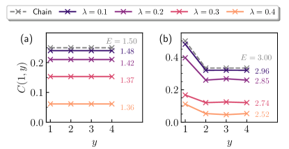
Figure 2: Numerical results of the correlator $C\left(1,y\right)$ defined in Eq. (12) for systems with different numbers of fermions and parameters $\lambda$. The lattice sizes and Hubbard interaction strengths are all $(N_{x},N_{y})=(5,4)$ and $U=1.5$. The number of fermions in (a) and (b) is two ($\uparrow\downarrow$) and four ($\uparrow\uparrow\downarrow\downarrow$), respectively. For comparison, the correlators for a bipartite chain are also plotted (dashed lines). The corresponding energies are indicated to the right of each line.

To verify the existence of the $\eta$-pairing edge states $|\psi_{\text{{edge}}}\rangle$, we study the system $H_{2\text{{D}}}$ in two- and four-fermion subspaces with Hubbard interaction $U$ through exact diagonalization. To characterize the $\eta$-pairing edge states, we introduce the following correlator [27, 15]

$$C\left(y^{\prime},y\right)=\langle\psi_{\text{{edge}}}|\eta_{x=1,y^{\prime}}^{{\dagger}}\eta_{x=1,y}|\psi_{\text{{edge}}}\rangle,$$ (12)

where $\eta_{x,y}=\left(-1\right)^{y}c_{x,y,\downarrow}c_{x,y,\uparrow}$. The lattice index $x$ is fixed at the left end in Eq. (12), because the lattice possesses inversion symmetry, and for an edge state, the correlator should vanish in the bulk. For the eigenstate $|\psi_{\text{{edge}}}\rangle$ possessing ODLRO, the correlator $C\left(y^{\prime},y\right)$ is a constant when $\left|y^{\prime}-y\right|$ increases. This is a characteristic of superconductivity. When $\lambda\approx 0$, the presence of $\eta$-pairing edge states is clear; the two chains at the boundaries, which support the edge states, are isolated from the bulk of the cylinder, and the boundary chains can be regarded as approximate bipartite lattices. For the $\eta$-pairing state $\left|\psi(n)\right\rangle=(\eta^{{\dagger}})^{n}|\mathrm{vac}\rangle$ in a bipartite lattice, the correlator is [15]

$$C\left(y^{\prime},y\right)=\frac{n\left(N_{y}-n\right)}{N_{y}\left(N_{y}-1\right)},y^{\prime}\neq y.$$ (13)

This bipartite lattice corresponds to the isolated chain with $N_{y}$ sites at the boundary.

The $\eta$-pairing edge states are bound pairs localized at the boundary, which have substantial pairing energy and near-zero kinetic energy; thus, the pair density at the boundary $\mathcal{N}_{\text{{edge}}}=\sum_{y}\langle\psi_{\text{{edge}}}|n_{1,y,\uparrow}n_{1,y,\downarrow}|\psi_{\text{{edge}}}\rangle$ is useful in the search for the $\eta$-pairing edge states. One can search for $\eta$-pairing edge states in eigenstates with large $\mathcal{N}_{\text{{edge}}}$. We perform the numerical calculation for systems with different numbers of particles and parameters $\lambda$.

The numerical results of the correlator $C\left(y^{\prime},y\right)$ for the $\eta$-pairing edge states are shown in Fig. 2. The corresponding local particle density is presented in Appendix C. The lattice size of the system is set as $(N_{x},N_{y})=(5,4)$, where $N_{x}$ is truncated to an odd number such that the edge states appear in only one boundary. The interaction strength is $U=1.5$, and the number of particles are two (one spin up and one spin down, marked as $\uparrow\downarrow$), and four ($\uparrow\uparrow\downarrow\downarrow$) for Figs. 2(a) and (b), respectively. In the invariant subspaces of two and four fermions, there exist only one $\eta$-pairing state with one-pairing and two-pairing, respectively. A higher filling ratio will involve the bulk fermions, which have no contribution to the ODLRO. The correlators of a uniform chain in Eq. (13) are plotted as a comparison. One can see that until $\lambda=0.4$, these two states have the long-range correlation of $C\left(1,y\right)$. The comparison between the energies of two and four fermions indicates that there is no interaction between the paired fermions in small $\lambda$ limit, which is equivalent to finite $\left|\lambda\right|<1$ with large $N_{x}$. In Appendix C, we also give the numerical results of three fermions, and the approximate results of even- and odd-number fermions in a larger system. In these cases, the previous conclusions are still valid.

IV Resonant transmission

In the preceding section, we demonstrate the existence of the $\eta$-pairing edge states from the correlator. A natural question is that whether system $H_{\mathrm{2D}}$ supports a two-fluid state containing single fermions and $\eta$ pairs localized at the boundary of the system. We attempt to answer this question and demonstrate the properties of the two-fluid edge states.

Particle beam scattering is a conventional technique for detecting the nature of matter [36]. Because no scattering occurs between the single fermions and $\eta$ pairs, resonant transmission provides a means to present the features of two-fluid edge states. The detection of resonant transmission for a many-body state is somewhat challenging, both theoretically and experimentally. Nevertheless, exceptional point (EP) [30, 31, 32] dynamics in non-Hermitian quantum mechanics can reduce the difficulty of the calculation. For a system with parameters at EP, two or more eigenvalues along with their associated eigenstates become identical, leading to unidirectional dynamics. This allows us to employ EP dynamics to simulate the perfect resonant transmission of particles. It can shorten the lengths of the input and output leads, and the scattering process in a Hermitian system can be effectively treated as the dynamics of a non-Hermitian system (see Appendix D). In the following, we present the resonant transmission dynamics of the two-fluid edge states. For comparison, the scattering dynamics between a single fermion and an FM edge state are also examined.

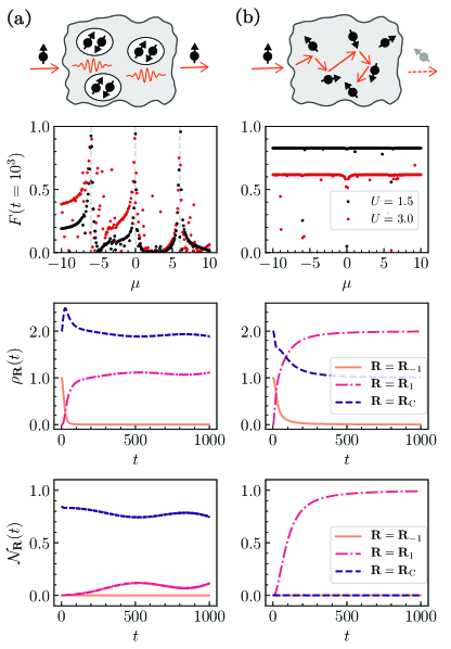
Figure 3: (a) Resonant transmission process. (b) Ordinary scattering process. The top panel is a schematic of the two processes. The bottom panel presents the corresponding numerical results of fidelity defined in Eq. (15) at time $t=1000$ as a function of $\mu$ for $U=1.5$ and $3$, as well as the particle density $\rho_{\mathbf{R}}(t)$ and the pair density $\mathcal{N}_{\mathbf{R}}(t)$ defined in Eqs. (16) and (17) for parameters $\mu=0$ and $U=1.5$. The other parameters are $(N_{x},N_{y})=(5,4)$, $\lambda=0.2$ and $J=0.1$. The scales of the Hamiltonian and time $t$ are taken as dimensionless.

We consider the dynamics in a non-Hermitian system, which consists of the 2D SSH Hubbard model $H_{2\text{{D}}}$ and two extra sites (with indexes $j=-1$ and $1$), connected by the unidirectional hopping

$$H_{\text{{NH}}} = H_{2\text{{D}}}+J\sum_{\sigma=\uparrow,\downarrow}\left(c_{\alpha,\sigma}^{\dagger}c_{-1,\sigma}+c_{1,\sigma}^{\dagger}c_{\beta,\sigma}\right)$$ (14)

$$+\mu\sum_{\sigma=\uparrow,\downarrow}\sum_{j=\pm 1}c_{j,\sigma}^{\dagger}c_{j,\sigma},$$

where $c_{\alpha,\sigma}^{\dagger}$ and $c_{\beta,\sigma}$ are fermion operators at the edge of the cylinder $H_{2\text{{D}}}$. A schematic of the system configuration is presented in Appendix D. When $\mu=E^{\mathrm{L/R}}=6\cos k_{y}$ is considered, a Jordan block with order of three should appear in single-particle subspace (see Appendix D). For the many-body case, if the two-fluid states remain eigenstates of $H_{2\text{{D}}}$, it still supports the Jordan block with order of three. This can be verified by examining the dynamic process. We take the initial state as $\left|\psi(0)\right\rangle=c_{-1,\uparrow}^{\dagger}|\psi_{\text{{edge}}}^{\mathrm{a}}\rangle$, with the AFM $\eta$-pairing edge state $|\psi_{\text{{edge}}}^{\mathrm{a}}\rangle$ satisfying $s^{2}|\psi_{\text{{edge}}}^{\mathrm{a}}\rangle=0$, and calculate the time evolution $\left|\psi(t)\right\rangle=e^{-iH_{\text{{NH}}}t}\left|\psi(0)\right\rangle/|e^{-iH_{\text{{NH}}}t}\left|\psi(0)\right\rangle|$. The expected final state is $\left|\psi_{\mathrm{final}}\right\rangle=c_{1,\uparrow}^{\dagger}|\psi_{\text{{edge}}}^{\mathrm{a}}\rangle$ when resonant transmission occurs. Here, the numerical computations are performed by using a uniform mesh in conducting time discretization.

To characterize the procedure, we introduce three quantities: the fidelity between the expected state and the evolved state

$$F(t)=\left|\left\langle\psi_{\mathrm{final}}\right.\left|\psi(t)\right\rangle\right|;$$ (15)

the particle density of the evolved state at different spatial regions

$$\rho_{\mathbf{R}}(t)=\sum_{\mathbf{r=R}}\sum_{\sigma=\uparrow,\downarrow}\left\langle\psi(t)\right|n_{\mathbf{r},\sigma}\left|\psi(t)\right\rangle,$$ (16)

where $\mathbf{R}=\mathbf{R}_{-1}$ and $\mathbf{R}_{1}$ respectively represent the extra sites with indexes $j=-1$ and $1$, and $\mathbf{R}=\mathbf{R}_{\mathrm{C}}$ represents the sites of the scattering center $H_{2\text{{D}}}$; and the pair density

$$\mathcal{N}_{\mathbf{R}}(t)=\sum_{\mathbf{r=R}}\left\langle\psi(t)\right|n_{\mathbf{r},\uparrow}n_{\mathbf{r},\downarrow}\left|\psi(t)\right\rangle.$$ (17)

Figure. 3(a) presents the numerical results of the fidelity after a sufficiently long time as a function of $\mu$, and the two other quantities as functions of time $t$. As expected, the peaks appear at $\mu=-6$, $0$ and $6$, where the single fermion is resonantly transmitted from site $\mathbf{R}_{-1}$ to site $\mathbf{R}_{1}$. This can also be seen in the particle density $\rho_{\mathbf{R}}(t)$ and the pair density $\mathcal{N}_{\mathbf{R}}(t)$ for $\mu=0$ and $U=1.5$.

For comparison, in Fig. 3(b), we consider the time evolution of another initial state $\left|\psi(0)\right\rangle=c_{-1,\uparrow}^{\dagger}|\psi_{\text{{edge}}}^{\mathrm{b}}\rangle$, with the FM edge state $|\psi_{\text{{edge}}}^{\mathrm{b}}\rangle$ satisfying$\ s^{2}|\psi_{\text{{edge}}}^{\mathrm{b}}\rangle=2$, $s_{z}|\psi_{\text{{edge}}}^{\mathrm{b}}\rangle=0$, and the state $\left|\psi_{\mathrm{final}}\right\rangle=c_{1,\uparrow}^{\dagger}|\psi_{\text{{edge}}}^{\mathrm{b}}\rangle$. The numerical results indicate that the single fermion is scattered by the $\mathrm{FM}$ state $|\psi_{\text{{edge}}}^{\mathrm{b}}\rangle$ at any $\mu$ value due to the Hubbard interaction. When $\mu=0$ and $U=1.5$, two fermions are transmitted to site $\mathbf{R}_{1}$ after a sufficiently long time.

V Summary

We present a concept of topologically protected two-fluid edge states and a means for their detection. We demonstrate the existence of such states in the 2D SSH Hubbard model, which provides an analog to the topological insulator. Such a material behaves as a conductor in its interior but possesses a surface containing superconducting states. In other words, the condensation of $\eta$ pairs can exist only on the surface of the material. We also determine that a two-fluid state can be formed as a many-body eigenstate of a realistic Hubbard model. By employing EP dynamics, a technique of the numerical simulation is developed to overcome the computational difficulty in the scattering problem of many-body system, which involve numerous basis vectors. It is expected to measure the resonant transmission in experiment via peaks in transmission coefficient [37, 38]. At present, the possible experimental implementation to explore the two-fluid edge states is ultracold fermions in an optical lattice [39].

Appendix

In this Appendix, we present A. Symmetries, FM and AFM eigenstates for $H_{0}$; B. Solution of the extended 2D SSH model; C. More exact numerical results and approximate numerical results; and D. Non-Hermitian description of resonant transmission.

A Symmetries, FM and AFM eigenstates for $H_{0}$

Considering the Hubbard Hamiltonian $H_{0}$ in the main text, one can defined two sets of pseudo-spin operators ($s^{\pm},s^{z}$) and ($\eta^{\pm},\eta^{z}$). The first set is

$$s^{+} = \left(s^{-}\right)^{\dagger}=\sum_{\mathbf{r}}s_{\mathbf{r}}^{+},$$

$$s^{z} = \sum_{\mathbf{r}}s_{\mathbf{r}}^{z},$$ (A1)

where the local operators $s_{\mathbf{r}}^{+}=c_{\mathbf{r},\uparrow}^{\dagger}c_{\mathbf{r},\downarrow}$ and $s_{\mathbf{r}}^{z}=\left(n_{\mathbf{r},\uparrow}-n_{\mathbf{r},\downarrow}\right)/2$ obey the Lie algebra, i.e., $[s_{\mathbf{r}}^{+},$ $s_{\mathbf{r}}^{-}]=2s_{\mathbf{r}}^{z}$, and $[s_{\mathbf{r}}^{z},$ $s_{\mathbf{r}}^{\pm}]=\pm s_{\mathbf{r}}^{\pm}$. The second set is

$$\eta^{+} = \left(\eta^{-}\right)^{\dagger}=\sum_{\mathbf{r}}\eta_{\mathbf{r}}^{+},$$

$$\eta^{z} = \sum_{\mathbf{r}}\eta_{\mathbf{r}}^{z},$$ (A2)

with $\eta_{\mathbf{r}}^{+}=c_{\mathbf{r},\uparrow}^{\dagger}c_{\mathbf{r},\downarrow}^{{\dagger}}$ ($-c_{\mathbf{r},\uparrow}^{\dagger}c_{\mathbf{r},\downarrow}^{{\dagger}}$) for $\mathbf{r}\in A$ ($\mathbf{r}\in B$), and $\eta_{\mathbf{r}}^{z}=\left(n_{\mathbf{r},\uparrow}+n_{\mathbf{r},\downarrow}-1\right)/2$ satisfying commutation relation $[\eta_{\mathbf{r}}^{+},$ $\eta_{\mathbf{r}}^{-}]=2\eta_{\mathbf{r}}^{z}$, and $[\eta_{\mathbf{r}}^{z},$ $\eta_{\mathbf{r}}^{\pm}]=\pm\eta_{\mathbf{r}}^{\pm}$. Straightforward algebra shows the symmetries of $H_{0}$:

$$\left[H_{0},s^{\pm}\right]=\left[H_{0},s^{z}\right]=0,$$ (A3)

and

$$\left[H_{0}-U\eta^{z},\eta^{\pm}\right]=\left[H_{0},\eta^{z}\right]=0,$$ (A4)

which will be employed to construct eigenstates of the Hamiltonian.

Starting from the diagonalization form of $H_{0}$ with zero $U$,

$$H_{0}(U=0)=\sum_{\mathbf{k},\sigma=\uparrow,\downarrow}\varepsilon_{\mathbf{k}}c_{\mathbf{k},\sigma}^{\dagger}c_{\mathbf{k},\sigma},$$ (A5)

one can construct an $m$-fermion FM eigenstate of $H_{0}(U\neq 0)$

$$\left|\psi_{\mathrm{FM}}(m,m)\right\rangle=\prod_{\left\{\mathbf{k}\right\}}^{m}c_{\mathbf{k},\uparrow}^{\dagger}\left|\mathrm{Vac}\right\rangle,$$ (A6)

with $\left|\mathrm{Vac}\right\rangle$ being the vacuum state of fermion $c_{\mathbf{r},\sigma}$, since the $U$ term has no effect on the fermions with aligned spin polarization. The symmetry in Eq. (A3) permits the existence of eigenstates

$$\left|\psi_{\mathrm{FM}}(m,l)\right\rangle=\left(s^{-}\right)^{\left(m-l\right)/2}\prod_{\left\{\mathbf{k}\right\}}^{m}c_{\mathbf{k},\uparrow}^{\dagger}\left|\mathrm{Vac}\right\rangle,$$ (A7)

with $l=-m,-m+2,...,m-4,m-2,m$, which obeys

$$H_{0}\left|\psi_{\mathrm{FM}}(m,l)\right\rangle=\sum_{\left\{\mathbf{\ k}\right\}}^{m}\varepsilon_{\mathbf{k}}\left|\psi_{\mathrm{FM}}(m,l)\right\rangle.$$ (A8)

These states are referred to as FM states since they obey

$$s^{2}\left|\psi_{\mathrm{FM}}(m,l)\right\rangle=\frac{m}{2}(\frac{m}{2}+1)\left|\psi_{\mathrm{FM}}(m,l)\right\rangle,$$ (A9)

and

$$s^{z}\left|\psi_{\mathrm{FM}}(m,l)\right\rangle=\frac{l}{2}\left|\psi_{\mathrm{FM}}(m,l)\right\rangle.$$ (A10)

Similarly, one can construct a set of AFM eigenstates based on the symmetry in Eq. (A4). An $n$-pair has the form

$$\left|\psi_{\mathrm{AFM}}(n)\right\rangle=\left(\eta^{+}\right)^{n}\left|\mathrm{Vac}\right\rangle,$$ (A11)

which obeys

$$H_{0}\left|\psi_{\mathrm{AFM}}(n)\right\rangle=nU\left|\psi_{\mathrm{AFM}}(n)\right\rangle,$$ (A12)

and

$$s^{2}\left|\psi_{\mathrm{AFM}}(n)\right\rangle=0.$$ (A13)

Obviously, an $\eta$-pairing state is spin singlet. In the main text, a two-fluid eigenstates is constructed based on the above two types of states.

B Solution of the extended 2D SSH model

Taking the periodic boundary condition in both directions, the interaction-free 2D SSH Hamiltonian in $\mathbf{k}$ space can be written as

$$H_{2\text{{D}}}(U=0)=\sum_{\mathbf{k}}\sum_{\sigma=\uparrow,\downarrow}\left(\begin{array}[]{cc}a_{\mathbf{k,}\sigma}^{{\dagger}}&b_{\mathbf{k,}\sigma}^{{\dagger}}\end{array}\right)h_{\mathbf{k}}\left(\begin{array}[]{c}a_{\mathbf{k,}\sigma}\\ b_{\mathbf{k,}\sigma}\end{array}\right),$$ (B1)

where the core matrix is

$$h_{\mathbf{k}}=\left(\begin{array}[]{cc}6\cos k_{y}&\vartheta_{\mathbf{k}}\\ \vartheta_{\mathbf{k}}^{\ast}&6\cos k_{y}\end{array}\right),$$ (B2)

with $\vartheta_{\mathbf{k}}=\left(\lambda+e^{-ik_{x}}\right)\left(3+2\cos k_{y}\right)$, based on the Fourier transformation

$$\left(a_{\mathbf{k,}\sigma},b_{\mathbf{k,}\sigma}\right)=\left(N_{x}N_{y}\right)^{-1/2}\sum_{\mathbf{r}}\left(c_{2x-1,y,\sigma},c_{2x,y,\sigma}\right)e^{-i\mathbf{k\cdot r}}.$$ (B3)

We note that the system satisfies time reversal symmetry and is invariant under the inversion symmetry

$$\mathcal{T}h_{\mathbf{k}}\mathcal{T}^{-1}\mathcal{=}h_{-\mathbf{k}},Rh_{\mathbf{k}}R^{-1}=h_{-\mathbf{k}},$$ (B4)

where $\mathcal{T}=K$ is conjugation operator and $R=\left(\begin{array}[]{cc}0&1\\ 1&0\end{array}\right)$. The eigenvectors of $h_{\mathbf{k}}$ are

$$\left|\psi_{\mathbf{k}}^{\pm}\right\rangle=\frac{1}{\sqrt{2}}\left(\begin{array}[]{c}\pm e^{i\theta_{\mathbf{k}}}\\ 1\end{array}\right),$$ (B5)

with $\theta_{\mathbf{k}}=\arg\left(\vartheta_{\mathbf{k}}\right)$ and the corresponding eigenvalues

$$E_{\mathbf{k}}^{\pm}=6\cos k_{y}\pm\left|3+2\cos k_{y}\right|\Lambda_{\mathbf{k}}.$$ (B6)

Here factor $\Lambda_{\mathbf{k}}=\sqrt{\lambda^{2}+1+2\lambda\cos k_{x}}$ determines the pseudo band gap, which vanishes at $k_{x}=0,\pi$ when taking $\lambda=\pm 1$.

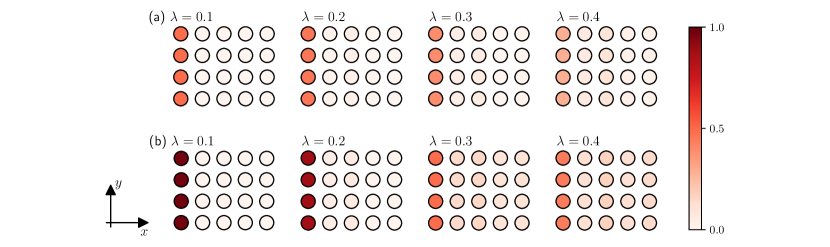
Figure 4: Numerical results for local particle density $\rho\left(\mathbf{r}\right)$ defined in Eq. (C1) for the systems with different numbers of fermions and parameters $\lambda$ . The lattices size and Hubbard interaction strength are all $(N_{x},N_{y})=(5,4)$ and $U=1.5$. The numbers of fermions are two ($\uparrow\downarrow$) and four ($\uparrow\uparrow\downarrow\downarrow$) for (a) and (b), respectively.

Under cylindrical boundary condition (taking open boundary condition in $x$ direction), this model supports topological edge states protected by time reversal symmetry and inversion symmetry. We introduce the wave polarization to characterize the topological phase transition [40, 41]

$$\mathbf{P}^{\pm}=\frac{1}{\left(2\pi\right)^{2}}\iint_{\mathrm{BZ}}\mathbf{A}_{\mathbf{k}}^{\pm}dk_{x}dk_{y},$$ (B7)

where $\mathbf{A}_{\mathbf{k}}^{\pm}=\langle\psi_{\mathbf{k}}^{\pm}|i\partial_{\mathbf{k}}|\psi_{\mathbf{k}}^{\pm}\rangle$ is the Berry connection, and the integral region is in the first Brillouin zone. We simply have

$$\mathbf{A}_{\mathbf{k}}^{\pm}=-\frac{1}{2}\hat{x}\partial_{k_{x}}\theta_{\mathbf{k}},$$ (B8)

and

$$\mathbf{P}^{\pm}=-\frac{1}{2}\hat{x}\mathcal{W}=\frac{1}{2}\hat{x}\left\{\begin{array}[]{cc}1,&\left|\lambda\right|<1\\ 0,&\left|\lambda\right|>1\end{array}\right..$$ (B9)

The topological characterization is obvious since

$$\mathcal{W}=\frac{1}{2\pi}\int_{-\pi}^{\pi}\partial_{k_{x}}\arg\left(\vartheta_{\mathbf{k}}\right)dk_{x}$$ (B10)

is essentially the winding number.

In the topologically nontrivial phase $\left|\lambda\right|<1$, we have nonzero polarization $\mathbf{P}^{\pm}=\left(1/2,0\right)$, thus it is expected to observe the topological edge state in the boundary of $x$ direction when the cylindrical boundary condition is taken. In fact, it can be checked that in the large-$N_{x}$ limit, the system supports two degenerate edge modes

$$|\psi_{k_{y},\sigma}^{\mathrm{L}}\rangle = \Omega\sum_{x}\left(-\lambda\right)^{x-1}a_{x,k_{y},\sigma}^{{\dagger}}|\mathrm{Vac}\rangle,$$

$$|\psi_{k_{y},\sigma}^{\mathrm{R}}\rangle = \Omega\sum_{x}\left(-\lambda\right)^{N_{x}-x}b_{x,k_{y},\sigma}^{{\dagger}}|\mathrm{Vac}\rangle,$$ (B11)

with the eigenenergy $E^{\mathrm{L}/\mathrm{R}}=6\cos k_{y}$ and the normalization constant $\Omega=\sqrt{1-\lambda^{2}}$, where the inverse transformation is $\left(a_{x,k_{y},\sigma},b_{x,k_{y},\sigma}\right)=N_{y}^{-1/2}\sum_{y}\left(c_{2x-1,y,\sigma},c_{2x,y,\sigma}\right)e^{-ik_{y}y}$.

C More exact numerical results and approximate numerical results

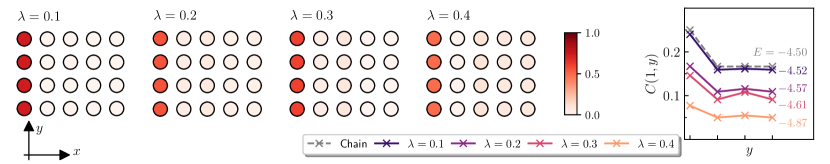
Figure 5: Numerical results of the local particle density $\rho\left(\mathbf{r}\right)$ and correlator $C\left(1,y\right)$ for the system with $3$ ($\uparrow\uparrow\downarrow$) fermions obtained from exact diagonalization. The lattices size and Hubbard interaction strength are all $(N_{x},N_{y})=(5,4)$ and $U=1.5$.

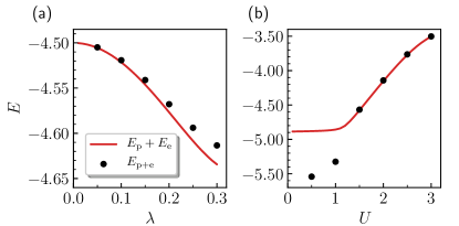
Figure 6: Comparison of energy $E_{\mathrm{p+e}}$ with $E_{\mathrm{p}}+E_{\mathrm{e}}$ obtained form exact diagonalization (a) as function of $\lambda$ with fixed $U=1.5$; (b) as function of $U$ with fixed $\lambda=0.2$. The lattices size is $(N_{x},N_{y})=(5,4)$.

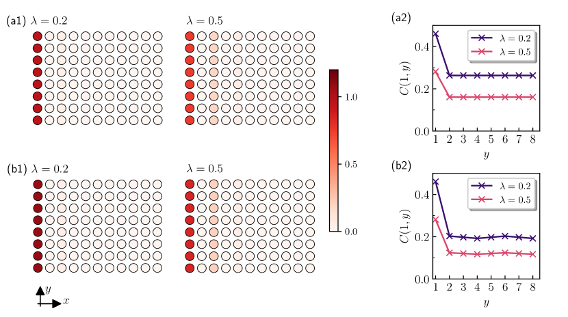
Figure 7: Numerical results obtained from the effective Hamiltonian in the subspace of edge states. (a1) and (b1) are local particle density $\rho\left(\mathbf{r}\right)$. (a2) and (b2) show correlator $C\left(1,y\right)$ for the systems with different numbers of fermions and parameters $\lambda$. The lattices size and Hubbard interaction strength are all $(N_{x},N_{y})=(11,8)$ and $U=1.5$. The numbers of fermions are $8$ ($4\uparrow 4\downarrow$) and $9$ ($5\uparrow 4\downarrow$ ); the energies are $E=6.00$ and $E=10.24$, for (a) and (b), respectively.

To visualize the distribution of the fermions of a state in real space, we calculate the local particle density

$$\rho\left(\mathbf{r}\right)=\sum_{\sigma=\uparrow,\downarrow}\langle\psi_{\text{{edge}}}|n_{\mathbf{r},\sigma}|\psi_{\text{{\ edge }}}\rangle.$$ (C1)

The numerical results of the local particle density $\rho\left(\mathbf{r}\right)$ for the $\eta$-pairing edge states with two and four fermions are presented in Figs. 4(a) and 4(b), which respectively correspond to the cases considered in Figs. 2(a) and 2(b) of the main text. In Fig. 5, we present the numerical results of the three-fermion ($\uparrow\uparrow\downarrow$) case. It indicates that the three-fermion $\eta$-pairing edge state also has off-diagonal long-range order. This is the simplest two-fluid edge state. We can gain some intuition in term of energy. We choose one of the three-fermion edge states with energy $E_{\mathrm{p+e}}$ from the numerical data. In Fig. 6, we present the comparison between the energy $E_{\mathrm{p+e}}$ and $E_{\mathrm{p}}+E_{\mathrm{e}}$, as functions of $\lambda$ [Fig. 6(a)] and $U$ [Fig. 6(b)], where $E_{\mathrm{p}}$ is the energy of $\eta$-pairing edge state in two-fermion subspace and $E_{\mathrm{e}}$ is the energy of a single-fermion edge state. It indicates that the energy $E_{\mathrm{p+e}}$ has the form of $E_{\mathrm{p}}+E_{\mathrm{e}}$ for small $\lambda$ or large $U$. This suggests the existence of the two-fluid edge states in certain parameter region.

To handle a larger system, we can write the matrix of effective Hamiltonian in the edge-states subspace. For the extended 2D SSH Hubbard model with zero $U$, there are two kinds of single-particle states: edge states $|\psi_{k_{y},\sigma}^{\mathrm{L/R}}\rangle$ and bulk states $|\psi_{k_{y},\sigma}^{\mathrm{bulk}}\rangle$, in the topologically nontrivial phase with $\left|\lambda\right|<1$. The wave function of an edge state exponential decay from edge to bulk, then the spatial overlap of these two states tends to zero in the thermodynamic limit, that is $|\langle\psi_{k_{y},\sigma}^{\mathrm{\ L/R}}|n_{\mathbf{r},\sigma}|\psi_{k_{y}^{\prime},\sigma}^{\mathrm{bulk}}\rangle|\rightarrow 0$ for any $\mathbf{r}$. Since the Hubbard interaction $U\sum_{\mathbf{r}}n_{\mathbf{r},\uparrow}n_{\mathbf{r},\downarrow}$ is local, when it is switched on, it does not hybridize these two kinds of states approximately, that is $\sum_{\mathbf{r}}|n_{\mathbf{r},\sigma}n_{\mathbf{r},\sigma^{\prime}}|\psi_{k_{y},\sigma}^{\mathrm{L/R}}\rangle|\psi_{k_{y}^{\prime},\sigma^{\prime}}^{\mathrm{bulk}}\rangle|\approx 0$ $\left(\sigma\neq\sigma^{\prime}\right)$. The main hybridization occurs between the bulk states, or the edge states. Notably, this approximation is more effective when $N_{x}$ is larger. Then we can consider the physics in the invariant subspace of edge states $\{|\psi_{k_{y},\sigma}^{\mathrm{L/R}}\rangle\}$, which has bipartite lattice symmetry that ensures the formation of two-fluid edge states. Based on this approximation, the $\eta$-pairing edge states in a larger system can be calculated approximately. In Figs. 7 (a) and 7(b), we present the numerical results with $8$ and $9$ fermions on the lattice with size $(N_{x},N_{y})=(11,8)$, respectively, obtained from the effective Hamiltonian in the subspace of edge states. We can see that for the cases of more fermions in a larger system, the $\eta$-pairing and two-fluid edge states with off-diagonal long-range order still exist.

D Non-Hermitian description of resonant transmission

In this section, we establish a connection between the resonant transmission of a scattering center and the EP dynamics of a non-Hermitian system, which is consisted with the scattering center and two extra sites. Two systems are schematically illustrated in Fig. 8(a) and 8(b). We consider a general scattering system by a single-particle Hamiltonian

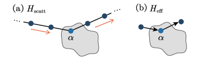
Figure 8: (a) Schematic illustration of the Hermitian system $H_{\mathrm{scatt}}$ in Eq. (D1). The orange arrows represent the wave of resonant transmission. (b) Schematic illustration of the effective non-Hermitian system $H_{\mathrm{eff}}$ in Eq. (D5). The black arrows indicate the unidirectional hoppings. The gray areas represent two identical scattering centers $H_{\mathrm{c}}$.

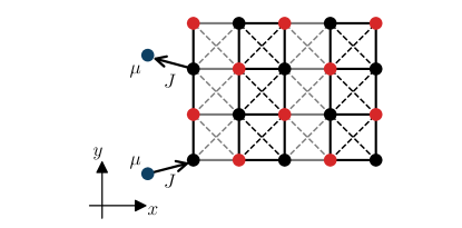
Figure 9: Schematic illustration of the configuration of the non-Hermitian Hamiltonian $H_{\text{{NH}}}$ considered in the main text. The blue dots represent two extra sites with on-site potential of strength $\mu$. The arrows indicate the unidirectional hopping of strength $J$.

$$H_{\mathrm{scatt}}=H_{\mathrm{Ld}}+H_{\mathrm{c}},$$ (D1)

where $H_{\mathrm{Ld}}$ represents the two leads,

$$H_{\mathrm{Ld}} = J\sum_{j=1}^{\infty}\left(\left|-j\right\rangle\left\langle-j-1\right|+\left|j\right\rangle\left\langle j+1\right|\right)$$

$$+J\left(\left|-1\right\rangle\left\langle\alpha\right|+\left|1\right\rangle\left\langle\alpha\right|\right)+\mathrm{\ H.c.}+\mu\sum_{\left|j\right|=1}^{\infty}\left|j\right\rangle\left\langle j\right|,$$

while $H_{\mathrm{c}}$ is a scattering center of $N$ sites,

$$H_{\mathrm{c}}=\sum_{q=1}^{N}\varepsilon_{q}\left|\phi_{q}\right\rangle\left\langle\phi_{q}\right|.$$ (D3)

Here $\alpha$ represents a site in the cluster $H_{\mathrm{c}}$ connecting to the left and right leads. $\left|\phi_{q}\right\rangle$ denotes the normalized eigenstate of $H_{\mathrm{c}}$ with energy $\varepsilon_{q}$. Now we consider the case, in which $H_{\mathrm{c}}$ has an isolated energy level at $q=\rho$, satisfying $\mu=\varepsilon_{\rho}$ and $\left|\varepsilon_{\rho}-\varepsilon_{\rho\pm 1}\right|\gg J$. It can be checked that the state $|\psi_{\pi/2}\rangle$ in the form

$$|\psi_{\pi/2}\rangle=\left\{\begin{array}[]{cc}e^{-i\pi j/2}\left|j\right\rangle,&\left|j\right|\geqslant 1\\ \gamma\left|\phi_{\rho}\right\rangle,&j\in\left\{\mathrm{c}\right\}\end{array}\right.,$$ (D4)

is an eigenstate of $H_{\mathrm{scatt}}$ with energy $\varepsilon_{\rho}$. where $\left\{\mathrm{c}\right\}$ denotes the set of index for the sites of scattering center. Here $\gamma$ is a complex number, determined by $\left\langle\alpha\right|\phi_{\rho}\rangle=\gamma^{-1}$.

In parallel, we consider a non-Hermitian Hamiltonian

$$H_{\mathrm{eff}} = J\left(\left|\alpha\right\rangle\left\langle-1\right|+\left|1\right\rangle\left\langle\alpha\right|\right)$$ (D5)

$$+\sum_{q=1}^{N}\varepsilon_{q}\left|\phi_{q}\right\rangle\left\langle\phi_{q}\right|+\mu\sum_{j=\pm 1}\left|j\right\rangle\left\langle j\right|,$$

which contains two unidirectional hopping terms. For the isolated energy level with $\left|\varepsilon_{\rho}-\varepsilon_{\rho\pm 1}\right|\gg J$, it reduces to

$$H_{\mathrm{eff}} \approx J\left(\left|\alpha\right\rangle\left\langle-1\right|+\left|1\right\rangle\left\langle\alpha\right|\right)$$ (D6)

$$+\varepsilon_{\rho}\left|\phi_{\rho}\right\rangle\left\langle\phi_{\rho}\right|+\mu\sum_{j=\pm 1}\left|j\right\rangle\left\langle j\right|.$$

Under the resonant condition $\mu=\varepsilon_{\rho}$ the dynamics is governed by the Jordan block with order of three

$$M_{\mathrm{JB}}=\left(\begin{array}[]{ccc}\mu&0&0\\ J&\mu&0\\ 0&J&\mu\end{array}\right).$$ (D7)

For initial state $\left|\psi(0)\right\rangle=\left|-1\right\rangle=\left(1,0,0\right)^{\mathrm{T}}$, the final state is $\left|\psi(\infty)\right\rangle=\left|1\right\rangle=\left(0,0,1\right)^{\mathrm{T}}$, due to the fact

$$\exp\left(-iM_{\mathrm{JB}}t\right)$$

$$= \exp\left(-i\mu t\right)\left[1-i\left(M_{\mathrm{JB}}-\mu\right)t-\frac{1}{2}\left(M_{\mathrm{JB}}-\mu\right)^{2}t^{2}\right],$$

and

$$\exp\left(-iM_{\mathrm{JB}}t\right)\left(\begin{array}[]{c}1\\ 0\\ 0\end{array}\right)=\exp\left(-i\mu t\right)\left(\begin{array}[]{c}1\\ -iJt\\ -\frac{1}{2}J^{2}t^{2}\end{array}\right).$$ (D8)

A straightforward implication of the result is that this process accords with the resonant transmission, i.e., the particle is perfectly transported from the left to the right.

Nevertheless, we would like to point that no matter if it is resonant or not, the Jordan block always exists, but with different order. Here we consider the case of $\mu$ deviate from $\varepsilon_{\rho}$, and the dynamics is governed by the matrix

$$M=\left(\begin{array}[]{ccc}\mu&0&0\\ J&\varepsilon_{\rho}&0\\ 0&J&\mu\end{array}\right)\text{.}$$ (D9)

Here matrix $M$ can be related to the Jordan block with order of two, which is $\left(\begin{array}[]{ccc}\mu&0&0\\ 1&\mu&0\\ 0&0&\varepsilon_{\rho}\end{array}\right)$, by Jordan decomposition. The time evolution is

$$\exp\left(-iMt\right)\left(\begin{array}[]{c}1\\ 0\\ 0\end{array}\right)=\exp\left(-i\mu t\right)\left(\begin{array}[]{c}1\\ \varsigma\tau\\ \varsigma^{2}\left[\tau+i\left(\varepsilon_{\rho}-\mu\right)t\right]\end{array}\right),$$ (D10)

where $\varsigma=J/\left(\varepsilon_{\rho}-\mu\right)$ and $\tau=\exp\left[-i\left(\varepsilon_{\rho}-\mu\right)t\right]-1$.

It indicates that in the resonant case, the evolved state converges to the target state more rapidly. In other word, to distinguish two different processes, we can observe the fidelity between the evolved state and the target state for two different dynamics processes at the same sufficiently long time $t$.

In Fig. 9, we present the schematic illustration of the system configuration of the Hamiltonian in Eq. (13) of the main text.

References

- Klitzing et al. [1980] K. v. Klitzing, G. Dorda, and M. Pepper, New method for high-accuracy determination of the fine-structure constant based on quantized hall resistance, Phys. Rev. Lett. 45, 494 (1980).
- Laughlin [1981] R. B. Laughlin, Quantized Hall conductivity in two dimensions, Phys. Rev. B 23, 5632 (1981).
- Thouless et al. [1982] D. J. Thouless, M. Kohmoto, M. P. Nightingale, and M. den Nijs, Quantized Hall conductance in a two-dimensional periodic potential, Phys. Rev. Lett. 49, 405 (1982).
- Niu et al. [1985] Q. Niu, D. J. Thouless, and Y.-S. Wu, Quantized Hall conductance as a topological invariant, Phys. Rev. B 31, 3372 (1985).
- Chiu et al. [2016] C.-K. Chiu, J. C. Y. Teo, A. P. Schnyder, and S. Ryu, Classification of topological quantum matter with symmetries, Rev. Mod. Phys. 88, 035005 (2016).
- Zhang and Song [2021] K. L. Zhang and Z. Song, Quantum phase transition in a quantum Ising chain at nonzero temperatures, Phys. Rev. Lett. 126, 116401 (2021).
- Bistritzer and MacDonald [2011] R. Bistritzer and A. H. MacDonald, Moiré bands in twisted double-layer graphene, Proceedings of the National Academy of Sciences 108, 12233 (2011).
- Wu et al. [2018] F. Wu, T. Lovorn, E. Tutuc, and A. H. MacDonald, Hubbard model physics in transition metal dichalcogenide moiré bands, Phys. Rev. Lett. 121, 026402 (2018).
- Wong et al. [2020] D. Wong, K. P. Nuckolls, M. Oh, B. Lian, Y. Xie, S. Jeon, K. Watanabe, T. Taniguchi, B. A. Bernevig, and A. Yazdani, Cascade of electronic transitions in magic-angle twisted bilayer graphene, Nature 582, 198 (2020).
- Xu and Balents [2018] C. Xu and L. Balents, Topological superconductivity in twisted multilayer graphene, Phys. Rev. Lett. 121, 087001 (2018).
- Peri et al. [2021] V. Peri, Z.-D. Song, B. A. Bernevig, and S. D. Huber, Fragile topology and flat-band superconductivity in the strong-coupling regime, Phys. Rev. Lett. 126, 027002 (2021).
- Xie and MacDonald [2020] M. Xie and A. H. MacDonald, Nature of the correlated insulator states in twisted bilayer graphene, Phys. Rev. Lett. 124, 097601 (2020).
- Cao et al. [2018a] Y. Cao, V. Fatemi, S. Fang, K. Watanabe, T. Taniguchi, E. Kaxiras, and P. Jarillo-Herrero, Unconventional superconductivity in magic-angle graphene superlattices, Nature 556, 43 (2018a).
- Cao et al. [2018b] Y. Cao, V. Fatemi, A. Demir, S. Fang, S. L. Tomarken, J. Y. Luo, J. D. Sanchez-Yamagishi, K. Watanabe, T. Taniguchi, E. Kaxiras, et al., Correlated insulator behaviour at half-filling in magic-angle graphene superlattices, Nature 556, 80 (2018b).
- Yang [1989] C. N. Yang, pairing and off-diagonal long-range order in a Hubbard model, Phys. Rev. Lett. 63, 2144 (1989).
- Rosch et al. [2008] A. Rosch, D. Rasch, B. Binz, and M. Vojta, Metastable superfluidity of repulsive fermionic atoms in optical lattices, Phys. Rev. Lett. 101, 265301 (2008).
- Strohmaier et al. [2010] N. Strohmaier, D. Greif, R. Jördens, L. Tarruell, H. Moritz, T. Esslinger, R. Sensarma, D. Pekker, E. Altman, and E. Demler, Observation of elastic doublon decay in the Fermi-Hubbard model, Phys. Rev. Lett. 104, 080401 (2010).
- Sensarma et al. [2010] R. Sensarma, D. Pekker, E. Altman, E. Demler, N. Strohmaier, D. Greif, R. Jördens, L. Tarruell, H. Moritz, and T. Esslinger, Lifetime of double occupancies in the Fermi-Hubbard model, Phys. Rev. B 82, 224302 (2010).
- Hofmann and Potthoff [2012] F. Hofmann and M. Potthoff, Doublon dynamics in the extended Fermi-Hubbard model, Phys. Rev. B 85, 205127 (2012).
- Kaneko et al. [2019] T. Kaneko, T. Shirakawa, S. Sorella, and S. Yunoki, Photoinduced pairing in the Hubbard model, Phys. Rev. Lett. 122, 077002 (2019).
- Tindall et al. [2019] J. Tindall, B. Buča, J. R. Coulthard, and D. Jaksch, Heating-induced long-range pairing in the Hubbard model, Phys. Rev. Lett. 123, 030603 (2019).
- Tisza [1938] L. Tisza, Transport phenomena in Helium II, Nature 141, 913 (1938).
- Landau [1941] L. Landau, Theory of the superfluidity of Helium II, Phys. Rev. 60, 356 (1941).
- Ginzburg and Landau [2009] V. L. Ginzburg and L. D. Landau, On the theory of superconductivity, in On Superconductivity and Superfluidity (Springer, 2009) pp. 113–137.
- Bardeen et al. [1957] J. Bardeen, L. N. Cooper, and J. R. Schrieffer, Theory of superconductivity, Phys. Rev. 108, 1175 (1957).
- Su et al. [1979] W. P. Su, J. R. Schrieffer, and A. J. Heeger, Solitons in polyacetylene, Phys. Rev. Lett. 42, 1698 (1979).
- Yang [1962] C. N. Yang, Concept of off-diagonal long-range order and the quantum phases of liquid He and of superconductors, Rev. Mod. Phys. 34, 694 (1962).
- Bender and Boettcher [1998] C. M. Bender and S. Boettcher, Real spectra in non-Hermitian Hamiltonians having PT symmetry, Phys. Rev. Lett. 80, 5243 (1998).
- Mostafazadeh [2002] A. Mostafazadeh, Pseudo-hermiticity versus PT symmetry: the necessary condition for the reality of the spectrum of a non-Hermitian Hamiltonian, Journal of Mathematical Physics 43, 205 (2002).
- Müller and Rotter [2008] M. Müller and I. Rotter, Exceptional points in open quantum systems, Journal of Physics A: Mathematical and Theoretical 41, 244018 (2008).
- Heiss [2012] W. Heiss, The physics of exceptional points, Journal of Physics A: Mathematical and Theoretical 45, 444016 (2012).
- Rotter and Bird [2015] I. Rotter and J. Bird, A review of progress in the physics of open quantum systems: theory and experiment, Reports on Progress in Physics 78, 114001 (2015).
- Lin et al. [2014] S. Lin, X. Z. Zhang, and Z. Song, Sudden death of particle-pair Bloch oscillation and unidirectional propagation in a one-dimensional driven optical lattice, Phys. Rev. A 90, 063411 (2014).
- Yang and Zhang [1990] C. N. Yang and S. C. Zhang, SO4 symmetry in a Hubbard model, Modern Physics Letters B 4, 759 (1990).
- Singh and Scalettar [1991] R. R. P. Singh and R. T. Scalettar, Exact demonstration of pairing in the ground state of an attractive-U Hubbard model, Phys. Rev. Lett. 66, 3203 (1991).
- Jin and Song [2021] L. Jin and Z. Song, Symmetry-protected scattering in non-Hermitian linear systems, Chinese Physics Letters 38, 024202 (2021).
- Landauer [1957] R. Landauer, Spatial variation of currents and fields due to localized scatterers in metallic conduction, IBM Journal of research and development 1, 223 (1957).
- Nazarov et al. [2009] Y. V. Nazarov, Y. Nazarov, and Y. M. Blanter, Quantum transport: introduction to nanoscience (Cambridge university press, 2009).
- Mazurenko et al. [2017] A. Mazurenko, C. S. Chiu, G. Ji, M. F. Parsons, M. Kanász-Nagy, R. Schmidt, F. Grusdt, E. Demler, D. Greif, and M. Greiner, A cold-atom Fermi–Hubbard antiferromagnet, Nature 545, 462 (2017).
- Liu and Wakabayashi [2017] F. Liu and K. Wakabayashi, Novel topological phase with a zero Berry curvature, Phys. Rev. Lett. 118, 076803 (2017).
- Wu et al. [2020] H. C. Wu, L. Jin, and Z. Song, Nontrivial topological phase with a zero Chern number, Phys. Rev. B 102, 035145 (2020).