Homeomorphic Model for the Polyhedral Smash Product of Disks and Spheres

Abstract.

In this paper we present unpublished work by David Stone on polyhedral smash products. He proved that the polyhedral smash product of the CW-pair $(D^{2},S^{1})$ over a simplicial complex $K$ is homeomorphic to an iterated suspension of the geometric realization of $K$. Here we generalize his technique to the CW-pair $(D^{k+1},S^{k})$, for an arbitrary $k$. We generalize the result further to a set of disks and spheres of different dimensions.

1. Introduction

In all the following, $m\in{\mathbb{N}}$ is any natural number and $[m]=\{1,\cdots,m\}$. Also, we set $K$ to be an abstract simplicial complex whose vertex set is contained in $[m]$, that is $K$ is a family of subsets $\sigma\subseteq[m]$, called simplices, such that whenever $\sigma\in K$ and $\tau\subseteq\sigma$, then $\tau\in K$.

Definition 1.1 (Polyhedral smash product).

[3, Construction 8.3.1] Let $(\underline{X},\underline{A})=\{(X_{i},A_{i})\}_{i\in[m]}$ be a family of pointed CW-pairs, that is, the $X_{i}$ are CW-complexes and $A_{i}\hookrightarrow X_{i}$ are subcomplexes, for all $i\in[m]$. The polyhedral smash product of $(\underline{X},\underline{A})$ over $K$, denoted $\widehat{Z}(K;(\underline{X},\underline{A}))\subseteq\bigwedge_{i=1}^{m}X_{i}$, is the space given by

$$\widehat{Z}(K;(\underline{X},\underline{A}))=\bigcup_{\sigma\in K}\widehat{D}(\sigma),$$

(1) $$\text{where }\widehat{D}(\sigma)=\bigwedge_{i=1}^{m}Y_{i}\quad\text{with}\ Y_{i}=\begin{cases}X_{i}\ \text{if}\ i\in\sigma,\\ A_{i}\ \text{otherwise}\end{cases},\quad\forall\sigma\in K.$$

Using categorical language, consider $\textsc{Cat}(K)$ to be the face category of $K$, that is, objects are simplices and morphisms are inclusions. Define the $\textsc{Cat}(K)$-diagram given by

$$\widehat{D}:\textsc{Cat}(K) \to\text{Top}$$

(2) $$\sigma \mapsto\widehat{D}(\sigma),$$

where $\widehat{D}(\sigma)$ is given by $(\ref{dhat})$ and the functor $\widehat{D}$ maps the morphism $\rho\subseteq\sigma$ to the inclusion $\widehat{D}(\rho)\subseteq\widehat{D}(\sigma)$. Then

(3) $$\widehat{Z}(K;(\underline{X},\underline{A}))=\operatorname*{colim}_{\sigma\in K}\widehat{D}(\sigma).$$

Below we recall some well-known operations on spaces.

Definition 1.2.

[4, §0]   For $n\in{\mathbb{N}}$, let $(X,x_{0})$ and $(Y,y_{0})$ be two pointed topological spaces.

• The join $X\ast Y$ of $X$ and $Y$ is the quotient space defined by $X\ast Y=X\times Y\times I/\sim,$ where $I=[0,1]$ and $\sim$ is the equivalence relation generated by

  $$(x,y,0) \sim(x,y^{\prime},0),\ \forall x\in X\ \text{and}\ \forall y,y^{\prime}\in Y,$$

  $$(x,y,1) \sim(x^{\prime},y,1),\ \forall x,x^{\prime}\in X\ \text{and}\ \forall y\in Y.$$

• The wedge sum $X\vee Y$ of $X$ and $Y$ is the quotient space defined by $X\vee Y=X\amalg Y/(x_{0}\sim y_{0})$.

• The smash product $X\wedge Y$ of $X$ and $Y$ is the quotient space defined by $X\wedge Y=X\times Y/X\vee Y$.

• The (unreduced) suspension $\Sigma X$ of $X$ is the space defined by $\Sigma X=S^{0}\ast X$, where $S^{0}$ denotes the $0$-sphere.

• The (unreduced) cone $CX$ of $X$ is the space defined by $CX=c\ast X$, where $c$ is a single point.

David stone made the following conjecture.

Conjecture 1.3.

If $F$ is a compact subspace of ${\mathbb{R}}^{n}$, then there is a homeomorphism

$$\widehat{Z}(K;(c\ast\Sigma F,\Sigma F))\cong\Sigma\left(\operatorname*{\divideontimes}^{m}F\right)\ast|K|,$$

where $\operatorname*{\divideontimes}^{m}F$ is defined as the $m$-fold join of $m$ copies of $F$.

As it is mentioned in [1, Remark 2.20], David Stone used a kind of geometrical argument to prove a particular case of his conjecture by taking $F=S^{0}$. Hence he proved the following.

Theorem 1.4.

[5] There is a homeomorphism

$$\widehat{Z}(K;(D^{2},S^{1}))\cong\Sigma^{m+1}|K|.$$

In this paper we apply the same technique to a more general case. For $k\in{\mathbb{N}}$, we consider $F=S^{k-1}$, which is compact (as a closed and bounded subspace of ${\mathbb{R}}^{k}$), and we have $\Sigma F\cong S^{k}$, $c\ast\Sigma F\cong D^{k+1}$ and $\operatorname*{\divideontimes}^{m}F\cong S^{km-1}$ (since $S^{i}\ast S^{j}\cong S^{i+j+1}$). Hence

$$\left(\operatorname*{\divideontimes}^{m}F\right)\ast|K| \cong S^{km-1}\ast|K|$$

$$\cong\left(\operatorname*{\divideontimes}^{km}S^{0}\right)\ast|K|$$

$$\cong\Sigma^{km}|K|.$$

So we can state a generalization of Stone’s result.

Theorem 1.5.

For any $k\in{\mathbb{N}}\cup\{0\}$, there is a homeomorphism

$$\widehat{Z}(K;(D^{k+1},S^{k}))\cong\Sigma^{km+1}|K|.$$

The goal of this paper is first to generalize David Stone’s technique for the proof of Theorem 1.5 and secondly to provide a further generalization (see Theorem 6.6) of the latter result for a set of disks and spheres of different dimensions.

Theorem 1.6.

For any $m$-tuple $J=(j_{1},\cdots,j_{m})$ in $({\mathbb{N}}\cup\{0\})^{m}$, there is a homeomorphism

$$\widehat{Z}(K;(\underline{D^{J+1}},\underline{S^{J}}))\cong\Sigma^{j_{1}+\cdots+j_{m}+1}|K|,$$

where $\left(\underline{D^{J+1}},\underline{S^{J}}\right)=\left\{\left(D^{j_{1}+1},S^{j_{1}}\right),\cdots,\left(D^{j_{m}+1},S^{j_{m}}\right)\right\}$.

In order to prove Theorem 1.5 we need to put together some topological and combinatorial tools, hence the rest of the paper is organized as follows. In Sections 2 and 3, we describe respectively the necessary topological and combinatorial tools. Section 4 is devoted to the proof of Theorem 1.5, for $k\geq 1$. The case $k=0$, namely Theorem 5.1, is treated in Section 5 using a more categorical argument. Finally, in Section 6 we prove the main result, Theorem 6.6, using an inductive argument based on the case $k=0$.

Acknowledgments

I would like to thank the Fields Institute at the University of Toronto where I started this work during the Thematic Program on Toric Topology and Polyhedral Products, for the inspiring work environment and the valuable financial support. I am thankful to Anthony Bahri for sharing the private correspondence from David Stone with me. Also I would like to express my deep gratitude to both Donald Stanley and Martin Frankland for their scientific and financial contribution to the realization of this work. Finally, I am deeply grateful to the referee for the concrete idea and guideline regarding the methodology that helped me to build the entire Section 6.

2. Topological tools

Among the tools we use in the proof of Theorem 1.5, the homeomorphisms $\Psi:C\Delta^{n-1}\to C^{n}$ and $\overline{\Psi}:\Sigma\Delta^{n-1}\to\widetilde{D}^{n}$, described below, are both playing an important role. They were defined by David Stone in [5] and we recycle them here to prove this more general case. Before we introduce them, let us first recall the usual homeomorphism $\widetilde{\Theta}:CX/X\to\Sigma X$.

Given a space $X$, we identify $X$ with the base $c\times X\times\{1\}$ of $CX=c\ast X$. Set $S^{0}=\{s_{1},s_{2}\}$ to be the $0$-sphere and consider the map

$$\Theta:CX \to\Sigma X$$

$$[c,x,\lambda] \mapsto\Theta[c,x,\lambda]=\begin{cases}(s_{1},x,2\lambda),\ \text{if}\ 0\leq\lambda\leq\dfrac{1}{2}\\ (s_{2},x,2-2\lambda),\ \text{if}\ \dfrac{1}{2}\leq\lambda\leq 1.\end{cases}$$

Then $\Theta$ factors through a map $\widetilde{\Theta}:CX/X\to\Sigma X$; see Figure 1.

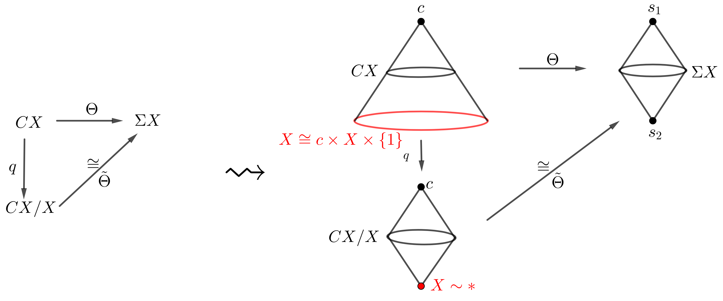
Figure 1. Factorization of $\Theta$ through $\widetilde{\Theta}$.

Lemma 2.1.

The map $\widetilde{\Theta}$ is a homeomorphism.

Notation 2.2.

In ${\mathbb{R}}^{n}$,

• let $e_{i}$ be the $i^{\text{th}}$ standard basis vector. Let $c$ denote the origin and let $t_{1},\cdots,t_{n}$ denote the coordinates of a point $x\in{\mathbb{R}}^{n}$. We identify $x\sim\overrightarrow{cx}$ and so $x=\sum_{i=1}^{n}t_{i}e_{i}$.

• Set $C=[0,2]$, with based point $2$ and consider

  $C^{n}=[0,2]^{n}=\left\{\sum_{i=1}^{n}t_{i}e_{i}\in{\mathbb{R}}^{n}:0\leq t_{i}\leq 2\right\}$, the $n$-cube of side $2$.

  $\partial_{+}C^{n}=\left\{\sum_{i=1}^{n}t_{i}e_{i}\in C^{n}:\max t_{i}=2\right\}$, the outer boundary of $C^{n}$.

  $\partial_{-}C^{n}=\left\{\sum_{i=1}^{n}t_{i}e_{i}\in C^{n}:\min t_{i}=0\right\}$, the inner boundary of $C^{n}$.

  $\partial C^{n}=\partial_{+}C^{n}\cup\partial_{-}C^{n}$, the boundary of $C^{n}$.

  $\widetilde{D}^{n}=C^{n}/\partial_{+}C^{n}$, with the quotient map $\omega:C^{n}\to\widetilde{D}^{n}$.

Lemma 2.3.

The quotient space $\widetilde{D}^{n}$ is a topological disk.

Proof.

Considering the CW-pair $(C^{n},\partial_{+}C^{n})$, we have

$$(C^{n},\partial_{+}C^{n}) \cong(c\ast\partial_{+}C^{n},\partial_{+}C^{n})$$

$$\cong(c\ast D^{n-1},D^{n-1}),$$

where the latter pair is the inclusion of the base of the cone $c\times D^{n-1}\times\{1\}\cong D^{n-1}\subseteq(c\ast D^{n-1})$. Hence collapsing the respective subspaces yields a homeomorphism

$$\widetilde{D}^{n}=C^{n}/\partial_{+}C^{n} \cong(c\ast D^{n-1})/D^{n-1}$$

$$\cong\Sigma D^{n-1}$$

$$\cong D^{n}.$$

Therefore $\widetilde{D}^{n}$ is a topological disk. ∎

Notation 2.4.

Let us consider the following setup.

• For any set $X=\{x_{1},\cdots,x_{p}\}\subseteq{\mathbb{R}}^{n}$, let $\text{cx}(X)$ denote the convex hull of $X$, that is

  $$\text{cx}(X)=\left\{\sum_{i=1}^{p}t_{i}x_{i}\in{\mathbb{R}}^{n}:t_{i}\geq 0,\sum_{i=1}^{p}t_{i}=1\right\}.$$

• Set $\Delta^{n-1}=\text{cx}\{e_{1},\cdots,e_{n}\}$ to be the standard $(n-1)$-simplex.

• For any $J\subseteq[n]$, set $\Delta(J)=\text{cx}\left(\{e_{i}:i\in J\}\right)\cong\Delta^{|J|-1}$, where $|J|$ denotes the cardinality of $J$.

Remark 2.5.

The abstract cone $C\Delta^{n-1}$ can be realized as a subspace of ${\mathbb{R}}^{n}$, a subspace which is homeomorphic to the $n$-cube $C^{n}$ by reparametrization as we can observe in Figure 2. This motivates the existence of a bijection $\Psi:C\Delta^{n-1}\to C^{n}$, defined by equation $(\ref{Psidef})$.

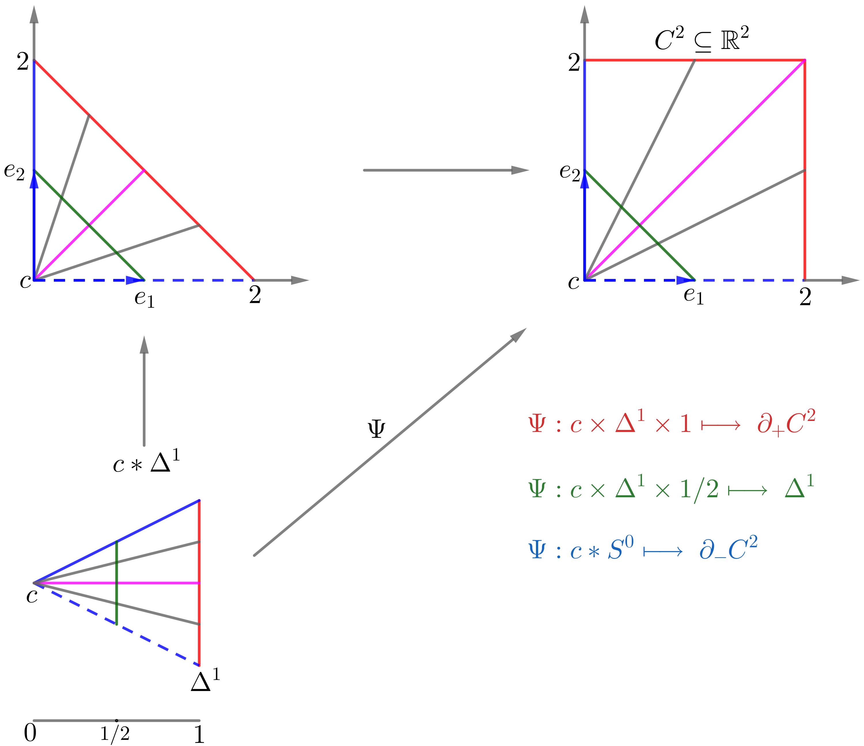
Figure 2. Illustration of the map $\Psi:C\Delta^{1}\to C^{2}$, that is for $n=2$.

For $x=\sum_{i=1}^{n}t_{i}e_{i}\in\Delta^{n-1}$, set $\overline{t}=\max\{t_{i}\}$, so $\overline{t}>0$. Define the map

(4) $$\Psi:C\Delta^{n-1} \to C^{n}$$

$$[c,x,\lambda] \mapsto\Psi[c,x,\lambda]=\begin{cases}2\lambda x,\ \text{if}\ 0\leq\lambda\leq\dfrac{1}{2}\\ \left((2-2\lambda)+(2\lambda-1)\dfrac{2}{\overline{t}}\right)x,\ \text{if}\ \dfrac{1}{2}\leq\lambda\leq 1,\end{cases}$$

where $C^{n}=[0,2]^{n}$ is the $n$-cube of side $2$ set in Notation 2.2.

Remark 2.6.

As mentioned in Notation 2.2, the basepoint of $C=[0,2]$ is $2$. The above defined map $\Psi$ does not send the cone point to the basepoint $(2,\cdots,2)$ of the $n$-cube $C^{n}$, as one might expect, but to the origin $c$ of ${\mathbb{R}}^{n}$ for convenience.

By Lemma 2.1, we have $C\Delta^{n-1}/\Delta^{n-1}\cong\Sigma\Delta^{n-1}\cong\Delta^{n}$. Also $\Psi(c\times\Delta^{n-1}\times\{1\})=\partial_{+}C^{n}$ and hence, $\Psi$ factors through the map

$$\overline{\Psi}:\Sigma\Delta^{n-1}\to\widetilde{D}^{n},$$

where $\widetilde{D}^{n}=C^{n}/\partial_{+}C^{n}$ is the topological disk introduced in Notation 2.2.

Lemma 2.7.

The maps $\Psi$ and $\overline{\Psi}$ are both homeomorphisms.

Proof.

As a continuous bijection from the compact space $C\Delta^{n-1}$ to the Hausdorff space $C^{n}$, $\Psi$ is a homeomorphism. Hence, $\Psi$ gives us the homeomorphism of the pairs $(C\Delta^{n-1},\Delta^{n-1})\cong(C^{n},\partial_{+}C^{n})$, so that the induced map $\overline{\Psi}:\Sigma\Delta^{n-1}\to\widetilde{D}^{n}$ is a homeomorphism. ∎

Remark 2.8.

If we consider $\left([0,2],2\right)$ to be a pointed space, then collapsing $\partial_{+}C^{2(k+1)}$ in $C^{2(k+1)}\cong C^{k+1}\times C^{k+1}$, we get $\widetilde{D}^{k+1}\bigwedge\widetilde{D}^{k+1}\cong D^{k+1}\bigwedge D^{k+1}\cong D^{2(k+1)}$. This can be generalized to the case of $C^{p(k+1)}\cong\underbrace{C^{k+1}\times\cdots\times C^{k+1}}_{p\ \text{times}}$ and so collapsing $\partial_{+}C^{p(k+1)}$ corresponds to $\bigwedge^{p}\widetilde{D}^{k+1}\cong\bigwedge^{p}D^{k+1}\cong D^{p(k+1)}$. Hence

$$\omega\left(\prod^{p}C^{k+1}\right)\cong\bigwedge^{p}\widetilde{D}^{k+1}\cong\bigwedge^{p}D^{k+1}\ \text{and}$$

$$\omega\left(\prod^{p}\partial_{-}C^{k+1}\right)\cong\bigwedge^{p}\partial\widetilde{D}^{k}\cong\bigwedge^{p}S^{k},\ \text{where}\ \partial\widetilde{D}^{k}\ \text{denotes the boundary of}\ \widetilde{D}^{k+1}.$$

Lemma 2.9.

For any compact and Hausdorff spaces $X$ and $Y$, there is a homeomorphism

$$\varphi:C(X\ast Y)\to CX\times CY.$$

Proof.

We follow the proof of [2, Lemma 8.1]. We can represent a point in $C(X\ast Y)$ by $[c,[x,y,t],\lambda]$. We define the homeomorphism $\varphi$ by

$$\varphi([c,[x,y,t],\lambda])=([c,x,2\lambda\cdot\min\{t,1/2\}],[c,y,2\lambda\cdot\min\{1-t,1/2\}])\in CX\times CY,$$

where the cone point is at $\lambda=0$. At $\lambda=1$, $\varphi$ reduces to the usual homeomorphism

$$X\ast Y\cong(CX\times Y)\cup(X\times CY).$$

The map $\varphi$ is a homeomorphism as a continuous bijection from the compact space $C(X\ast Y)$ to the Hausdorff space $CX\times CY$. ∎

3. Combinatorial tools

One of the main goals of this section is to embed the simplicial complex $K$ in a bigger simplex with vertex set $[(k+1)m]$. We start by introducing a linearized version of the join of spaces.

Definition 3.1 (Geometrically joinable).

 

• Two compact subspaces $X$ and $Y$ of ${\mathbb{R}}^{n}$ are said to be geometrically joinable if whenever $x,x^{\prime}\in X$, $y,y^{\prime}\in Y$ and $\lambda,\lambda^{\prime}\in I$ are such that $\lambda x+(1-\lambda)y=\lambda^{\prime}x^{\prime}+(1-\lambda^{\prime})y^{\prime}$, then we have one of the three following possibilities

  • $\lambda=\lambda^{\prime}=0$, and so $y=y^{\prime}$;

  • $\lambda=\lambda^{\prime}=1$, and so $x=x^{\prime}$;

  • $0\neq\lambda=\lambda^{\prime}\neq 1$, $x=x^{\prime}$ and $y=y^{\prime}$.

• More generally, $p$ compact subspaces $X_{1},\cdots,X_{p}\subseteq{\mathbb{R}}^{n}$ are geometrically joinable if whenever we have an equality between two convex combinations of points of $X_{1},\cdots,X_{p}$, that is, whenever

  $$\sum_{i=1}^{p}\lambda_{i}x_{i}=\sum_{i=1}^{p}\lambda_{i}^{\prime}x_{i}^{\prime},$$

  for some $x_{i},x_{i}^{\prime}\in X_{i}$ and $\lambda_{i},\lambda_{i}^{\prime}\in I$ with $\sum_{i=1}^{p}\lambda_{i}=1=\sum_{i=1}^{p}\lambda_{i}^{\prime}$, then for all $i=1,\cdots,p$ such that $\lambda_{i}\neq 0$ or $\lambda_{i}^{\prime}\neq 0$, we have $\lambda_{i}=\lambda_{i}^{\prime}$ and $x_{i}=x_{i}^{\prime}$.

• If $p$ compact subspaces $X_{1},\cdots,X_{p}\subseteq{\mathbb{R}}^{n}$ are geometrically joinable, then we define their geometric join $\operatorname*{\overline{\divideontimes}}_{i=1}^{p}X_{i}$ to be the set of all convex combinations of elements of $X_{i}$, that is,

  $$\operatorname*{\overline{\divideontimes}}_{i=1}^{p}X_{i}=\left\{\sum_{i=1}^{p}\lambda_{i}x_{i}\in{\mathbb{R}}^{n}:x_{i}\in X_{i}\ \text{and}\ \lambda_{i}\in I\ \text{such that}\ \sum_{i=1}^{p}\lambda_{i}=1\right\}.$$

The notion of geometrically joinable introduced here is also called “in general position”. In the following, when we use the notation $X\overline{\ast}Y$, it is to be understood that $X$ and $Y$ are indeed geometrically joinable.

Example 3.2.

Single points $X_{1}=\{x_{1}\},\cdots,X_{p}=\{x_{p}\}$ in ${\mathbb{R}}^{n}$ are geometrically joinable if and only if they are affinely independent. In that case, their geometric join $\operatorname*{\overline{\divideontimes}}_{i=1}^{p}X_{i}$ is their convex hull, which is a $(p-1)$-simplex, that is,

$$\operatorname*{\overline{\divideontimes}}_{i=1}^{p}X_{i}=\text{cx}\{x_{1},\cdots,x_{p}\}\cong\Delta^{p-1}.$$

Lemma 3.3.

 

1. Let $X$ and $Y$ be geometrical joinable subspaces of ${\mathbb{R}}^{n}$. The map

   $$\Phi:X\ast Y \to X\overline{\ast}Y$$

   $$[x,y,\lambda] \mapsto\lambda x+(1-\lambda)y$$

   is a homeomorphism.

2. More generally, for geometrically joinable subspaces $X_{1},\cdots,X_{p}$ of ${\mathbb{R}}^{n}$, the map

   $$\Phi_{p}:\operatorname*{\divideontimes}_{i=1}^{p}X_{i} \to\operatorname*{\overline{\divideontimes}}_{i=1}^{p}X_{i}$$

   $$[x_{i},\lambda_{i}]_{i=1}^{p} \mapsto\sum_{i=1}^{p}\lambda_{i}x_{i}$$

   is a homeomorphism.

Remark 3.4.

Observe that if $U$ and $V$ are respective subspaces of geometrically joinable spaces $X$ and $Y$, then $U$ is geometrically joinable to $V$.

Lemma 3.5.

Let $X,Y_{1}$ and $Y_{2}$ be three compact subspaces of ${\mathbb{R}}^{n}$. If $X$ is geometrically joinable to each $Y_{i}$ and

(5) $$X\overline{\ast}Y_{1}\cap X\overline{\ast}Y_{2}=X\overline{\ast}\left(Y_{1}\cap Y_{2}\right),$$

then $X$ is geometrically joinable to $Y_{1}\cup Y_{2}$.

Proof.

Let $x,x^{\prime}\in X$, $w,w^{\prime}\in Y_{1}\cup Y_{2}$ and $\lambda,\lambda^{\prime}\in I$ be such that

(6) $$\lambda x+(1-\lambda)w=\lambda^{\prime}x^{\prime}+(1-\lambda^{\prime})w^{\prime}.$$

If we have either $w,w^{\prime}\in Y_{1}$ or $w,w^{\prime}\in Y_{2}$, then there is nothing to show since $X$ is geometrically joinable to both $Y_{1}$ and $Y_{2}$. Without lost of generality suppose $w\in Y_{1}$ and $w^{\prime}\in Y_{2}$, and so $(\ref{gj2})$ gives us

$$X\overline{\ast}Y_{1}\ni\lambda x+(1-\lambda)w=\lambda^{\prime}x^{\prime}+(1-\lambda^{\prime})w^{\prime}\in X\overline{\ast}Y_{2}.$$

Then by $(\ref{int2})$, there are $x^{\prime\prime}\in X$, $w^{\prime\prime}\in Y_{1}\cap Y_{2}$ and $\lambda^{\prime\prime}\in I$ such that

(7) $$\lambda x+(1-\lambda)w= \lambda^{\prime\prime}x^{\prime\prime}+(1-\lambda^{\prime\prime})w^{\prime\prime},$$

(8) $$\lambda^{\prime}x^{\prime}+(1-\lambda^{\prime})w^{\prime}= \lambda^{\prime\prime}x^{\prime\prime}+(1-\lambda^{\prime\prime})w^{\prime\prime}.$$

If $\lambda^{\prime\prime}=0$ (respectively $\lambda^{\prime\prime}=1$) then

• $\lambda=0$ (respectively $\lambda=1$) and $w=w^{\prime\prime}$ (respectively $x=x^{\prime\prime}$) by $(\ref{gjw1})$, since $X$ and $Y_{1}$ are geometrically joinable.

• $\lambda^{\prime}=0$ (respectively $\lambda^{\prime}=1$) and $w^{\prime}=w^{\prime\prime}$ (respectively $x^{\prime}=x^{\prime\prime}$) by $(\ref{gjw2})$, since $X$ and $Y_{2}$ are geometrically joinable.

Thus $\lambda=0=\lambda^{\prime}$ and $w=w^{\prime}$ (respectively $\lambda=1=\lambda^{\prime}$ and $x=x^{\prime}$).

If $0\neq\lambda^{\prime\prime}\neq 1$ then

• $\lambda=\lambda^{\prime\prime}$ and, $x=x^{\prime\prime}$ and $w=w^{\prime\prime}$ by $(\ref{gjw1})$, since $X$ and $Y_{1}$ are geometrically joinable.

• $\lambda^{\prime}=\lambda^{\prime\prime}$ and, $x^{\prime}=x^{\prime\prime}$ and $w^{\prime}=w^{\prime\prime}$ by $(\ref{gjw2})$, since $X$ and $Y_{2}$ are geometrically joinable.

Thus $\lambda=\lambda^{\prime}$ and, $x=x^{\prime}$ and $w=w^{\prime}$. Therefore $X$ is geometrically joinable to $Y_{1}\cup Y_{2}$. ∎

Notation 3.6.

Now let $n=(k+1)m$ and for $i\in[m]$, consider the following notations:

• $v_{i}^{\ell}=e_{(k+1)(i-1)+\ell}$, for any $\ell=1,\cdots,k+1$,

• $a_{i}=\dfrac{1}{k+1}\sum_{\ell=1}^{k+1}v_{i}=\text{bar}\{v_{i}^{\ell}\}_{\ell=1}^{k+1}$, that is, $a_{i}$ is the barycenter of $\{v_{i}^{\ell}\}_{\ell=1}^{k+1}$,

• $\Delta_{i}=\text{cx}\left\{v_{i}^{\ell}\right\}_{\ell=1}^{k+1}$,

• $S_{i}=\partial\Delta_{i}$.

Lemma 3.7.

For any subset $\sigma\subseteq[m]$, the collections $\{\Delta_{i}\}_{i\in\sigma}$, $\{S_{i}\}_{i\in\sigma}$ and $\{a_{i}\}_{i\in\sigma}$ are respectively families of geometrically joinable compact subspaces of ${\mathbb{R}}^{n}$.

Proof.

Consider the following identity of convex combinations

(9) $$\sum_{i=1}^{|\sigma|}\lambda_{i}x_{i}=\sum_{i=1}^{|\sigma|}\lambda_{i}^{\prime}x_{i}^{\prime},$$

for some $x_{i},x_{i}^{\prime}\in\Delta_{i}$ and $\lambda_{i},\lambda_{i}^{\prime}\in I$ with $\sum_{i=1}^{k}\lambda_{i}=1=\sum_{i=1}^{k}\lambda_{i}^{\prime}$. The equation $(\ref{del1})$ is equivalent to

$$\sum_{i=1}^{|\sigma|}\sum_{\ell=1}^{k+1}\lambda_{i}t_{i}^{\ell}v_{i}^{\ell}=\sum_{i=1}^{|\sigma|}\sum_{\ell=1}^{k+1}\lambda_{i}^{\prime}s_{i}^{\ell}v_{i}^{\ell},$$

where $x_{i}=\sum_{\ell=1}^{k+1}t_{i}^{\ell}v_{i}^{\ell}$ and $x_{i}^{\prime}=\sum_{\ell=1}^{k+1}s_{i}^{\ell}v_{i}^{\ell}$ are convex combinations. Since $\{v_{i}^{\ell}:i\in\sigma,\ell=1,\cdots,k+1\}$ is affinely independent, then $\lambda_{i}t_{i}^{\ell}=\lambda_{i}^{\prime}s_{i}^{\ell}$, for all $i\in\sigma,\ell=1,\cdots,k+1$. Without loss of generality if $\lambda_{i}\neq 0$ (the proof is similar if we assume $\lambda_{i}^{\prime}\neq 0$), then $t_{i}^{\ell}=\dfrac{\lambda_{i}^{\prime}}{\lambda_{i}}s_{i}^{\ell}$. Hence we have

$$\sum_{\ell=1}^{k+1}t_{i}^{\ell}=1 \Rightarrow\sum_{\ell=1}^{k+1}\dfrac{\lambda_{i}^{\prime}}{\lambda_{i}}s_{i}^{\ell}=1$$

$$\Rightarrow\dfrac{\lambda_{i}^{\prime}}{\lambda_{i}}\sum_{\ell=1}^{k+1}s_{i}^{\ell}=1$$

$$\Rightarrow\dfrac{\lambda_{i}^{\prime}}{\lambda_{i}}=1,\ \text{since}\ \sum_{\ell=1}^{k+1}s_{i}^{\ell}=1$$

$$\Rightarrow\lambda_{i}^{\prime}=\lambda_{i}$$

$$\Rightarrow t_{i}^{\ell}=s_{i}^{\ell}\text{, for all}\ i\in\sigma,\ell=1,\cdots,k+1$$

$$\Rightarrow x_{i}=\sum_{\ell=1}^{k+1}t_{i}^{\ell}v_{i}^{\ell}=\sum_{\ell=1}^{k+1}s_{i}^{\ell}v_{i}^{\ell}=x_{i}^{\prime}$$

$$\Rightarrow x_{i}=x_{i}^{\prime}.$$

Therefore the collection $\{\Delta_{i}\}_{i\in\sigma}$ is geometrically joinable. As the collection of boundaries of disjoint $k$-simplices $\Delta_{i}$ in ${\mathbb{R}}^{n}$ respectively, $\{S_{i}\}_{i\in\sigma}$ is a family of geometrically joinable compact subspaces of ${\mathbb{R}}^{n}$. Likewise, the collection of barycenters $\{a_{i}\}_{i\in\sigma}$ of the $k$-simplices $\Delta_{i}$ is geometrically joinable. ∎

Notation 3.8.

For any $\sigma\subseteq[m]$ and by Lemma 3.7, consider the setting

• $J(\sigma)=\cup_{i\in\sigma}\{(k+1)(i-1)+\ell\}_{\ell=1}^{k+1}\subseteq[n]$,

• $\Delta_{\sigma}=\Delta(J(\sigma))=\operatorname*{\overline{\divideontimes}}_{i\in\sigma}\Delta_{i}$,

• $S_{\sigma}=\operatorname*{\overline{\divideontimes}}_{i\in\sigma}S_{i}$,

• $S_{\sigma}^{*}=\operatorname*{\overline{\divideontimes}}_{j\notin\sigma}S_{j}$,

• $a_{\sigma}=\text{cx}\{a_{i}:i\in\sigma\}$.

An example of this setup is illustrated in Figure 3.

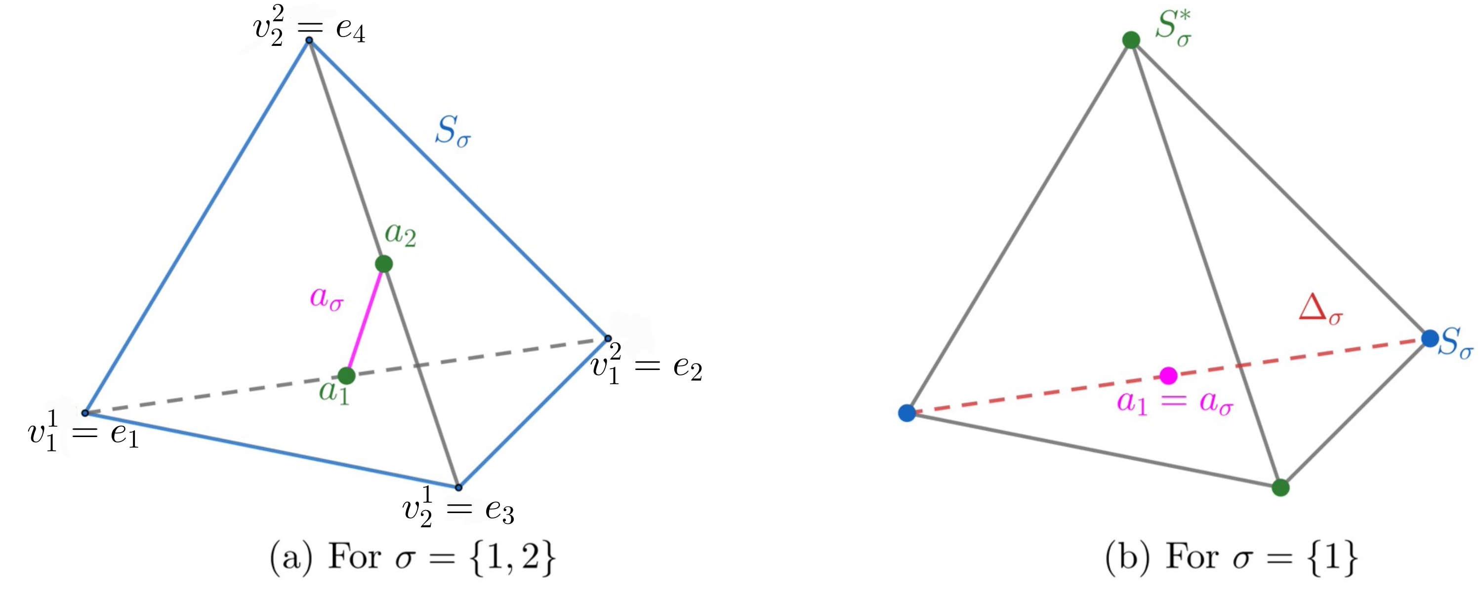
Figure 3. Examples of $a_{i}$, $S_{i}$, $a_{\sigma}$, $S_{\sigma}$ and $S^{*}_{\sigma}$, for $m=2$ and $k=1$, that is $n=4$.

Lemma 3.9.

For $\sigma\subseteq[m]$, the compact spaces $a_{\sigma}$ and $S_{\sigma}$ are geometrically joinable, and we have

$$\Delta_{\sigma}=a_{\sigma}\overline{\ast}S_{\sigma}.$$

Proof.

Let us prove $a_{\sigma}$ and $S_{\sigma}$ are geometrically joinable for $k=1$ and for $\sigma=\{1,2\}$; the general case can be proved similarly. In this setup, $S_{\sigma}$ can be split as follows

$$S_{\sigma}=\underbrace{[e_{1},e_{3}]}_{F_{1}}\cup\underbrace{[e_{1},e_{4}]}_{F_{2}}\cup\underbrace{[e_{2},e_{3}]}_{F_{3}}\cup\underbrace{[e_{2},e_{4}]}_{F_{4}}\ \text{and}$$

$$a_{\sigma}=\left[\dfrac{1}{2}e_{1}+\dfrac{1}{2}e_{2},\dfrac{1}{2}e_{3}+\dfrac{1}{2}e_{4}\right].$$

The complexes $a_{\sigma}$ and $F_{i}$, for each $i=1,2,3,4$, are both $1$-simplices and all their four vertices are not coplanar. So $a_{\sigma}$ and $F_{i}$, for each $i=1,2,3,4$, are geometrically joinable and their join $a_{\sigma}\overline{\ast}F_{i}$ is a $3$-simplex. Also we have

$$a_{\sigma}\overline{\ast}(F_{1}\cap F_{2})= a_{\sigma}\overline{\ast}\{e_{1}\}$$

$$= (a_{\sigma}\overline{\ast}F_{1})\cap(a_{\sigma}\overline{\ast}F_{2}).$$

Hence by Lemma 3.5, $a_{\sigma}$ is geometrically joinable to $F_{1}\cup F_{2}$. Similarly, we have

$$a_{\sigma}\overline{\ast}((F_{1}\cup F_{2})\cap F_{3})= a_{\sigma}\overline{\ast}\{e_{3}\}$$

$$= (a_{\sigma}\overline{\ast}(F_{1}\cup F_{2}))\cap(a_{\sigma}\overline{\ast}F_{3}).$$

Hence $a_{\sigma}$ is geometrically joinable to $F_{1}\cup F_{2}\cup F_{3}$. Similarly, we have

$$a_{\sigma}\overline{\ast}((F_{1}\cup F_{2}\cup F_{3})\cap F_{4})= a_{\sigma}\overline{\ast}\{e_{2},e_{4}\}$$

$$= (a_{\sigma}\overline{\ast}(F_{1}\cup F_{2}\cup F_{3}))\cap(a_{\sigma}\overline{\ast}F_{4}).$$

Hence $a_{\sigma}$ is geometrically joinable to $S_{\sigma}=F_{1}\cup F_{2}\cup F_{3}\cup F_{4}$.

For any $i\in[m]$, $S_{i}=\partial\Delta_{i}$ and $a_{i}=\text{bar}\{v_{i}^{\ell}\}_{\ell=1}^{k+1}$. Then $a_{i}$ and $S_{i}$ are geometrically joinable, and we have $\Delta_{i}=a_{i}\overline{\ast}S_{i}$. We deduce

$$\Delta_{\sigma} =\operatorname*{\overline{\divideontimes}}_{i\in\sigma}\Delta_{i}$$

$$=\operatorname*{\overline{\divideontimes}}_{i\in\sigma}(a_{i}\overline{\ast}S_{i})$$

$$=(\operatorname*{\overline{\divideontimes}}_{i\in\sigma}a_{i})\overline{\ast}(\operatorname*{\overline{\divideontimes}}_{i\in\sigma}S_{i})$$

$$=a_{\sigma}\overline{\ast}S_{\sigma}.\qed$$

4. Proof of Theorem 1.5

Now we have all the tools to write down the proof of Theorem 1.5 for $k\geq 1$. The case of $k=0$ will be treated in the next section. In the following, we consider the notations introduced in Sections 2 and 3.

Proof.

Setting $W_{\sigma}=\Delta_{\sigma}\overline{\ast}S_{\sigma}^{*}$ for each $\sigma\in K$, we have

(10) $$\bigcup_{\sigma\in K}W_{\sigma}=\bigcup_{\sigma\in K}\left(\left(\operatorname*{\overline{\divideontimes}}_{i\in\sigma}\Delta_{i}\right)\overline{\ast}\left(\operatorname*{\overline{\divideontimes}}_{j\notin\sigma}S_{j}\right)\right).$$

Consider the collection of simplices $A(K)=\{a_{\sigma}\}_{\sigma\in K}$, which is a geometric realization of the simplicial complex $K$ and

(11) $$|A(K)|=\bigcup_{\sigma\in K}a_{\sigma}$$

to be the underlying subspace of ${\mathbb{R}}^{n}={\mathbb{R}}^{(k+1)m}$. The complexes $a_{[m]}$ and $S_{[m]}$ are geometrically joinable by Lemma 3.9, and also $A(K)$ is a subcomplex of $a_{[m]}$. Therefore $|A(K)|$ and $S_{[m]}$ are geometrically joinable by Remark 3.4, and we have $S_{[m]}\overline{\ast}|A(K)|\cong S^{km-1}\ast|K|\cong\Sigma^{km}|K|$, since $S_{[m]}\cong S^{km-1}$. Then

$$W_{\sigma} =\Delta_{\sigma}\overline{\ast}S_{\sigma}^{*}$$

$$=a_{\sigma}\overline{\ast}(S_{\sigma}\overline{\ast}S_{\sigma}^{*})\ \text{by {Lemma \ref{gjs}}}$$

$$=a_{\sigma}\overline{\ast}S_{[m]}.$$

This is illustrated by Figure 4, where $W_{\sigma}$ is the union of the two blue triangular surfaces. In this example, we have $S_{[m]}\cong\partial W_{\sigma}$.

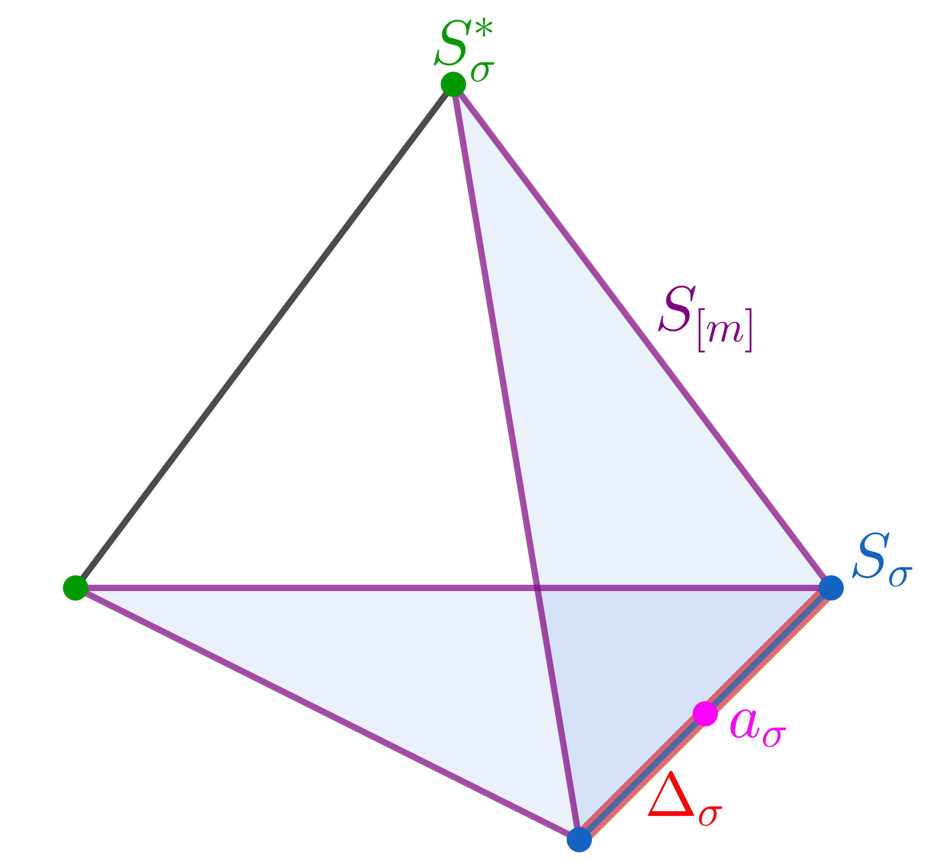
Figure 4. Examples of $W_{\sigma}$, for $m=2$, $\sigma=\{1\}$ and $k=1$, that is $n=4$.

Hence from equation (11) we also have

(12) $$\bigcup_{\sigma\in K}W_{\sigma}\cong\Sigma^{km}|K|.$$

Therefore we have

$$\Psi(C(\bigcup_{\sigma\in K}W_{\sigma})) \cong\bigcup_{\sigma\in K}\Psi(CW_{\sigma})$$

$$=\bigcup_{\sigma\in K}\Psi\left(C\left(\left(\operatorname*{\overline{\divideontimes}}_{i\in\sigma}\Delta_{i}\right)\overline{\ast}\left(\operatorname*{\overline{\divideontimes}}_{j\notin\sigma}S_{j}\right)\right)\right)\text{by (\ref{w1})}$$

$$\cong\bigcup_{\sigma\in K}\Psi\left(\prod_{i\in\sigma}(C\Delta_{i})\times\prod_{j\notin\sigma}(CS_{j})\right)\text{by {Lemma \ref{bbcg}}}$$

(13) $$\cong\bigcup_{\sigma\in K}\Psi\left(\prod_{i\in\sigma}C_{i}^{k+1}\times\prod_{j\notin\sigma}\partial_{-}C_{j}^{k+1}\right)\ \text{by {Lemma \ref{psi}},}$$

where $$C_{i}^{k+1} C_{j}^{k+1} (k+1)$$ and are copies of the -cube.

Then we get

$$\overline{\Psi}(\Sigma\bigcup_{\sigma\in K}W_{\sigma}) \cong\bigcup_{\sigma\in K}\overline{\Psi}(\Sigma W_{\sigma})$$

$$\cong\bigcup_{\sigma\in K}\ \omega\left(\prod_{i\in\sigma}C_{i}^{k+1}\times\prod_{j\notin\sigma}\partial_{-}C_{j}^{k+1}\right)\text{by}\ (\ref{pw1})\ \text{and}\ \textbf{Lemma \ref{psi}}$$

$$\cong\bigcup_{\sigma\in K}\ \left(\bigwedge_{i\in\sigma}\widetilde{D}_{i}^{k+1}\wedge\bigwedge_{j\notin\sigma}\partial\widetilde{D}_{i}^{k+1}\right)\text{by {Remark \ref{om}}, where $\widetilde{D}_{i}^{k+1}$ are copies of}$$

the nonstandard $$(k+1) \widetilde{D}^{k+1}$$-disk defined in Lemma 2.3.

$$\overline{\Psi}(\Sigma\bigcup_{\sigma\in K}W_{\sigma}) \cong\bigcup_{\sigma\in K}\ \left(\bigwedge_{i\in\sigma}D_{i}^{k+1}\wedge\bigwedge_{j\notin\sigma}S_{j}^{k}\right)\ \text{by {Lemma \ref{nsdisk}}, where $D_{i}^{k+1}$ and $S_{j}^{k}$ are copies of}$$

the $$(k+1) D^{k+1} k S^{k}$$-disk and the -sphere respectively

(14) $$\cong\widehat{Z}(K;(D^{k+1},S^{k})).$$

On the other hand, we obtain

$$\overline{\Psi}(\Sigma\bigcup_{\sigma\in K}W_{\sigma}) \cong\overline{\Psi}(\Sigma\Sigma^{km}|K|)\ \text{by (\ref{w2})}$$

$$\cong\overline{\Psi}\left(\Sigma^{km+1}|K|\right)$$

(15) $$\cong\Sigma^{km+1}|K|\ \text{by {Lemma \ref{psi}}.}$$

Therefore by $(\ref{pw2})$ and $(\ref{pw3})$, we have

$$\widehat{Z}(K;(D^{k+1},S^{k}))\cong\Sigma^{km+1}|K|.$$

Hence we have the result. ∎

5. The case $k=0$

In the previous section, we have proved Theorem 1.5 for $k\geq 1$. Here we prove the remaining case, namely $k=0$, given by the following.

Theorem 5.1.

There is a homeomorphism

$$\widehat{Z}(K;(D^{1},S^{0}))\cong\Sigma|K|.$$

For the purpose of the proof, we will consider the categorical definition of the polyhedral smash product given by $(\ref{psp})$. As in the third bullet of Notation 2.4, consider the functor

$$\Delta:\textsc{Cat}(K) \to\text{Top}$$

$$\sigma \mapsto\Delta(\sigma)\cong\Delta^{|\sigma|-1}.$$

The geometric realization of $K$ is given by

(16) $$|K|=\operatorname*{colim}_{\sigma\in K}\Delta(\sigma).$$

Proof.

Consider the composite functor $\Sigma\Delta$ given by

$$\Sigma\Delta:\textsc{Cat}(K) \to\text{Top}$$

$$\sigma \mapsto\Sigma\Delta(\sigma)\cong\Sigma\Delta^{|\sigma|-1}.$$

Let $\tau\subseteq\sigma$ be a face inclusion in $K$, with $|\tau|=p\leq\ell=|\sigma|$. We will look at the case $\tau=\{1,\cdots,p\}\subseteq\{1,\cdots,\ell\}=\sigma$ for simplicity; the same argument works for the general case. Consider the two following maps

$$\phi_{1}:C\Delta^{p-1} \to C\Delta^{\ell-1}$$

$$[c,(t_{1},\cdots,t_{p}),\lambda] \mapsto[c,(t_{1},\cdots,t_{p},\underbrace{0,\cdots,0}_{\ell-p\ \text{times}}),\lambda]$$

and

$$\phi_{2}:C^{p} \to C^{\ell}$$

$$(t_{1},\cdots,t_{p}) \mapsto(t_{1},\cdots,t_{p},\underbrace{0,\cdots,0}_{\ell-p\ \text{times}}).$$

The transformation $\overline{\Psi}:\Sigma\Delta\Rightarrow\widehat{D}$, where the functor $\widehat{D}$ is defined by $(\ref{dcat})$ for the pair $(D^{1},S^{0})$, is a natural isomorphism if the left hand side diagram commutes since it induces the commutative diagram on the right hand side below:

where $\overline{\phi}_{1}([s_{i},x,\lambda])=[\phi_{1}([c,x,\lambda])]$, for all $[s_{i},x,\lambda]\in\Sigma\Delta^{p-1}$, $\widetilde{D}^{p}=\underbrace{C^{1}\wedge\cdots\wedge C^{1}}_{p\ \text{times}}$ and so
$\overline{\phi}_{2}([y])=[\phi_{2}(y)]$, for all $y\in C^{p}$. For $[c,(t_{1},\cdots,t_{p}),\lambda]\in C\Delta^{p-1}$ we have

$$\Psi_{\ell}\phi_{1}([c,(t_{1},\cdots,t_{p}),\lambda]) =\Psi_{\ell}([c,(t_{1},\cdots,t_{p},\underbrace{0,\cdots,0}_{\ell-p\ \text{times}}),\lambda])$$

$$=\begin{cases}2\lambda(t_{1},\cdots,t_{p},\underbrace{0,\cdots,0}_{\ell-p\ \text{times}}),\ \text{if}\ 0\leq\lambda\leq\dfrac{1}{2}\\ \left((2-2\lambda)+(2\lambda-1)\dfrac{2}{\max_{1\leq i\leq p}\{t_{i}\}}\right)(t_{1},\cdots,t_{p},\underbrace{0,\cdots,0}_{\ell-p\ \text{times}}),\ \text{if}\ \dfrac{1}{2}\leq\lambda\leq 1\end{cases}\text{by (\ref{Psidef})}$$

$$\phi_{2}\Psi_{p}([c,(t_{1},\cdots,t_{p}),\lambda]) =\begin{cases}\phi_{2}(2\lambda(t_{1},\cdots,t_{p})),\ \text{if}\ 0\leq\lambda\leq\dfrac{1}{2}\\ \phi_{2}\left(\left((2-2\lambda)+(2\lambda-1)\dfrac{2}{\max_{1\leq i\leq p}\{t_{i}\}}\right)(t_{1},\cdots,t_{p})\right),\ \text{if}\ \dfrac{1}{2}\leq\lambda\leq 1\\ \end{cases}\text{by (\ref{Psidef})}$$

$$=\begin{cases}2\lambda(t_{1},\cdots,t_{p},\underbrace{0,\cdots,0}_{\ell-p\ \text{times}}),\ \text{if}\ 0\leq\lambda\leq\dfrac{1}{2}\\ \left((2-2\lambda)+(2\lambda-1)\dfrac{2}{\max_{1\leq i\leq p}\{t_{i}\}}\right)(t_{1},\cdots,t_{p},\underbrace{0,\cdots,0}_{\ell-p\ \text{times}}),\ \text{if}\ \dfrac{1}{2}\leq\lambda\leq 1.\end{cases}$$

Then the two diagrams commute and therefore $\overline{\Psi}$ is a natural isomorphism. Passing to the colimit, we have

(17) $$\operatorname*{colim}\overline{\Psi}:\operatorname*{colim}_{\sigma\in K}\Sigma\Delta(\sigma)\stackrel{{\scriptstyle\cong}}{{\longrightarrow}}\operatorname*{colim}_{\sigma\in K}\widehat{D}(\sigma).$$

But we have

$$\operatorname*{colim}_{\sigma\in K}\Sigma\Delta(\sigma)\cong\Sigma\operatorname*{colim}_{\sigma\in K}\Delta(\sigma)=\Sigma|K|\ \text{by (\ref{grK})}$$

and also considering identity $(\ref{psp})$, the homeomorphism $(\ref{col})$ yields a homeomorphism

$$\Sigma|K|\cong\widehat{Z}(K;(\underline{X},\underline{A})).\qed$$

6. Generalization of Theorem 1.5

In this section, we generalize Theorem 1.5 further, using an argument kindly provided by the referee. Instead of doubling all the vertices of $K$ simultaneously as in David Stone’s original construction, we double one vertex at a time and argue inductively, starting from the case $k=0$ in Theorem 5.1. Let us start by setting some notation and stating intermediate results.

Notation 6.1.

 

• For $J=(j_{1},\cdots,j_{m})$ an $m$-tuple from $({\mathbb{N}}\cup\{0\})^{m}$, denote the family of CW-pairs

  $$\left(\underline{D^{J+1}},\underline{S^{J}}\right)=\left\{\left(D^{j_{1}+1},S^{j_{1}}\right),\cdots,\left(D^{j_{m}+1},S^{j_{m}}\right)\right\}.$$

• Set $J_{i}=(0,\cdots,1,\cdots,0)$ to be the $m$-tuple having $1$ only at the $i$-th position and $0$ elsewhere. For a simplicial complex $K$ over $[m]$ and $i\in[m]$, consider the new simplicial complex $K(J_{i})$ with $m+1$ vertices labeled $\{1,\cdots,i-1,i_{a},i_{b},i+1,\cdots,m\}$ and defined by

  $$K(J_{i}) :=\ \{(\sigma\backslash\{i\})\cup\{i_{a},i_{b}\}\ |\ \sigma\in K\text{ and }i\in\sigma\}\cup\{\sigma\cup\{i_{a}\}\ |\ \sigma\in K\text{ and }i\notin\sigma\}$$

  $$\quad\cup\{\sigma\cup\{i_{b}\}\ |\ \sigma\in K\text{ and }i\notin\sigma\}\cup\{\text{all their subsets}\}.$$

The meaning behind the introduction of $K(J_{i})$ is illustrated in the following example.

Example 6.2.

For $m=2$, consider $K=\{\emptyset,\{1\},\{2\}\}$ and $J_{1}=(1,0)$. We have

$$\widehat{Z}(K;(\underline{D^{J_{1}+1}},\underline{S^{J_{1}}})) =\widehat{Z}(K;\{(D^{2},S^{1}),(D^{1},S^{0})\})$$

$$=\widehat{D}(\{1\})\cup\widehat{D}(\{2\})\quad\text{as a subspace of}\ D^{2}\wedge D^{1}$$

$$=D^{2}\wedge S^{0}\cup S^{1}\wedge D^{1}$$

$$\cong(D^{1}\wedge D^{1})\wedge S^{0}\cup(D^{1}\wedge S^{0}\cup S^{0}\wedge D^{1})\wedge D^{1}$$

$$=\left(D^{1}\wedge D^{1}\wedge S^{0}\right)\cup\left(D^{1}\wedge S^{0}\wedge D^{1}\right)\cup\left(S^{0}\wedge D^{1}\wedge D^{1}\right)$$

$$=\widehat{D}(\{1_{a},1_{b}\})\cup\widehat{D}(\{2\}\cup\{1_{a}\})\cup\widehat{D}(\{2\}\cup\{1_{b}\})$$

$$=\widehat{Z}(K(J_{1});\{(D^{1},S^{0}),(D^{1},S^{0}),(D^{1},S^{0})\})$$

$$=\widehat{Z}(K(J_{1});(D^{1},S^{0})),\ \text{see}\ \textsc{Figure}\ \ref{e63}.$$

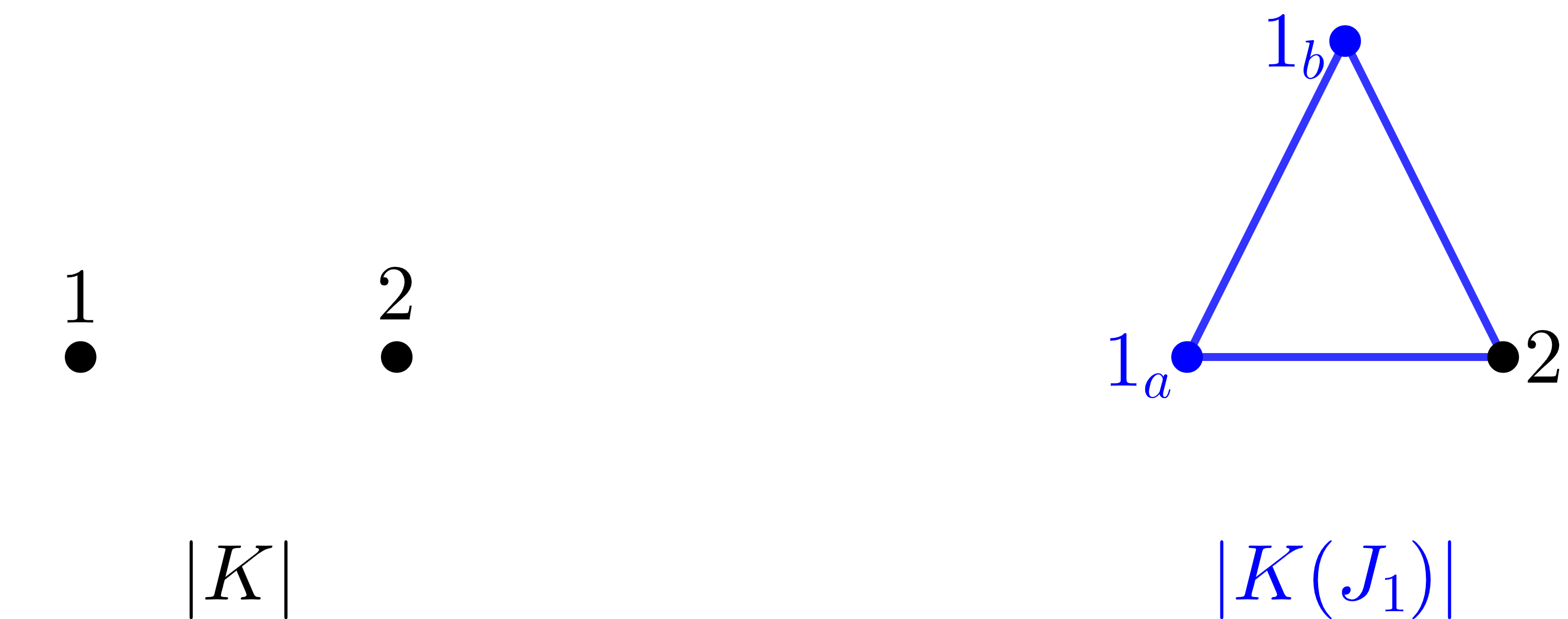
Figure 5. $K(J_{1})=\{\{1_{a},1_{b}\},\{1_{a},2\},\{1_{b},2\},\text{their subsets}\}$.

The next lemma suggests that the polyhedral smash product $\widehat{Z}(K;(\underline{D^{J+1}},\underline{S^{J}}))$ can be computed iteratively with steps involving $K(J_{i})$ for some $i\in[m]$.

Lemma 6.3.

Let $J=(j_{1},\cdots,j_{m})$ to be an $m$-tuple and $i\in[m]$ such that $j_{i}\neq 0$. There is a homeomorphism

$$\widehat{Z}(K;(\underline{D^{J+1}},\underline{S^{J}}))\cong\widehat{Z}(K(J_{i});(\underline{D^{J^{\prime}+1}},\underline{S^{J^{\prime}}})),$$

where $J^{\prime}$ is the $(m+1)$-tuple $J^{\prime}=(j_{1},\cdots,j_{i}-1,0,\cdots,j_{m})$.

Proof.

The polyhedral smash product $\widehat{Z}(K;(\underline{D^{J+1}},\underline{S^{J}}))$ is defined as follows

$$\widehat{Z}(K;(\underline{D^{J+1}},\underline{S^{J}})) =\widehat{Z}(K;\{(D^{j_{1}+1},S^{j_{1}}),\cdots,(D^{j_{i}+1},S^{j_{i}}),\cdots,(D^{j_{m}+1},S^{j_{m}})\})$$

$$=\bigcup_{\sigma\in K}\left(\widehat{D}(\sigma)\right)\quad\text{as a subspace of}\ \bigwedge_{\ell=1}^{m}D^{j_{\ell}+1}\cong\widetilde{D}^{j_{1}+\cdots+j_{m}+m}$$

$$=\bigcup_{\sigma\in K}\left(\bigwedge_{\ell=1}^{m}Y_{\ell}\right),\ \text{where}\ Y_{\ell}\ \text{depends on}\ \sigma\ \text{and is defined in}\ (\ref{dhat})$$

$$=\bigcup_{\sigma\in K,i\in\sigma}\left(\bigwedge_{\ell=1}^{m}Y_{\ell}\right)\cup\bigcup_{\sigma\in K,i\notin\sigma}\left(\bigwedge_{\ell=1}^{m}Y_{\ell}\right)$$

$$=\bigcup_{\sigma\in K,i\in\sigma}\left(Y_{1}\wedge\cdots\wedge D^{j_{i}+1}\wedge\cdots\wedge Y_{m}\right)\cup\bigcup_{\sigma\in K,i\notin\sigma}\left(Y_{1}\wedge\cdots\wedge S^{j_{i}}\wedge\cdots\wedge Y_{m}\right)$$

$$\cong\bigcup_{\sigma\in K,i\in\sigma}\left(Y_{1}\wedge\cdots\wedge(D^{j_{i}}\wedge D^{1})\wedge\cdots Y_{m}\right)$$

$$\quad\cup\bigcup_{\sigma\in K,i\notin\sigma}\left(Y_{1}\wedge\cdots\wedge(D^{j_{i}}\wedge S^{0}\cup S^{j_{i}-1}\wedge D^{1})\wedge\cdots Y_{m}\right)$$

$$=\bigcup_{\sigma\in K,i\in\sigma}\left(Y_{1}\wedge\cdots\wedge D^{j_{i}}\wedge D^{1}\wedge\cdots Y_{m}\right)\cup\bigcup_{\sigma\in K,i\notin\sigma}\left(Y_{1}\wedge\cdots\wedge D^{j_{i}}\wedge S^{0}\wedge\cdots Y_{m}\right)$$

$$\quad\cup\bigcup_{\sigma\in K,i\notin\sigma}\left(Y_{1}\wedge\cdots\wedge S^{j_{i}-1}\wedge D^{1}\wedge\cdots Y_{m}\right)$$

$$=\bigcup_{\sigma\in K,i\in\sigma}\widehat{D}\left((\sigma\backslash\{i\})\cup\{i_{a},i_{b}\}\right)\cup\bigcup_{\sigma\in K,i\notin\sigma}\widehat{D}\left(\sigma\cup\{i_{a}\}\right)\cup\bigcup_{\sigma\in K,i\notin\sigma}\widehat{D}\left(\sigma\cup\{i_{b}\}\right)$$

$$=\widehat{Z}\left(K(J_{i});\{(D^{j_{1}+1},S^{j_{1}}),\cdots,(D^{(j_{i}-1)+1},S^{j_{i}-1}),(D^{1},S^{0}),\cdots,(D^{j_{m}+1},S^{j_{m}})\}\right)$$

$$=\widehat{Z}(K(J_{i});(\underline{D^{J^{\prime}+1}},\underline{S^{J^{\prime}}})),$$

where $J^{\prime}$ is the $(m+1)$-tuple $J^{\prime}=(j_{1},\cdots,j_{i}-1,0,\cdots,j_{m})$. ∎

Example 6.4.

 

1. For $m=3$, consider $K=\{\{1,2\},\{3\},\text{their subsets}\}$ and $J=(1,1,0)$. We have

   $$\widehat{Z}(K;(\underline{D^{J+1}},\underline{S^{J}})) =\widehat{Z}(K;\{(D^{2},S^{1}),(D^{2},S^{1}),(D^{1},S^{0})\})$$

   $$=\widehat{D}(\{1,2\})\cup\widehat{D}(\{3\})\quad\text{as a subspace of}\ D^{2}\wedge D^{2}\wedge D^{1}$$

   $$=D^{2}\wedge D^{2}\wedge S^{0}\cup S^{1}\wedge S^{1}\wedge D^{1}$$

   $$\cong D^{2}\wedge(D^{1}\wedge D^{1})\wedge S^{0}\cup S^{1}\wedge(D^{1}\wedge S^{0}\cup S^{0}\wedge D^{1})\wedge D^{1}$$

   $$=\left(D^{2}\wedge D^{1}\wedge D^{1}\wedge S^{0}\right)\cup\left(S^{1}\wedge D^{1}\wedge S^{0}\wedge D^{1}\right)\cup\left(S^{1}\wedge S^{0}\wedge D^{1}\wedge D^{1}\right)$$

   $$=\widehat{D}((\{1,2_{a},2_{b}\})\cup\widehat{D}(\{2_{a},3\})\cup\widehat{D}(\{2_{b},3\})$$

   $$=\widehat{Z}(K(J_{2});\{(D^{2},S^{1}),(D^{1},S^{0}),(D^{1},S^{0}),(D^{1},S^{0})\})$$

   $$=\widehat{Z}(K(J_{2});(\underline{D^{J_{1}+1}},\underline{S^{J_{1}}})),\ \text{with}\ J_{1}=(1,0,0,0)$$

   $$=\widehat{Z}(K(J_{2})(J_{1});(D^{1},S^{0}))$$

   $$=\widehat{Z}(K(J);(D^{1},S^{0})),\ \text{where}\ K(J)=K(J_{2})(J_{1}).$$

   See Figure 6.

   

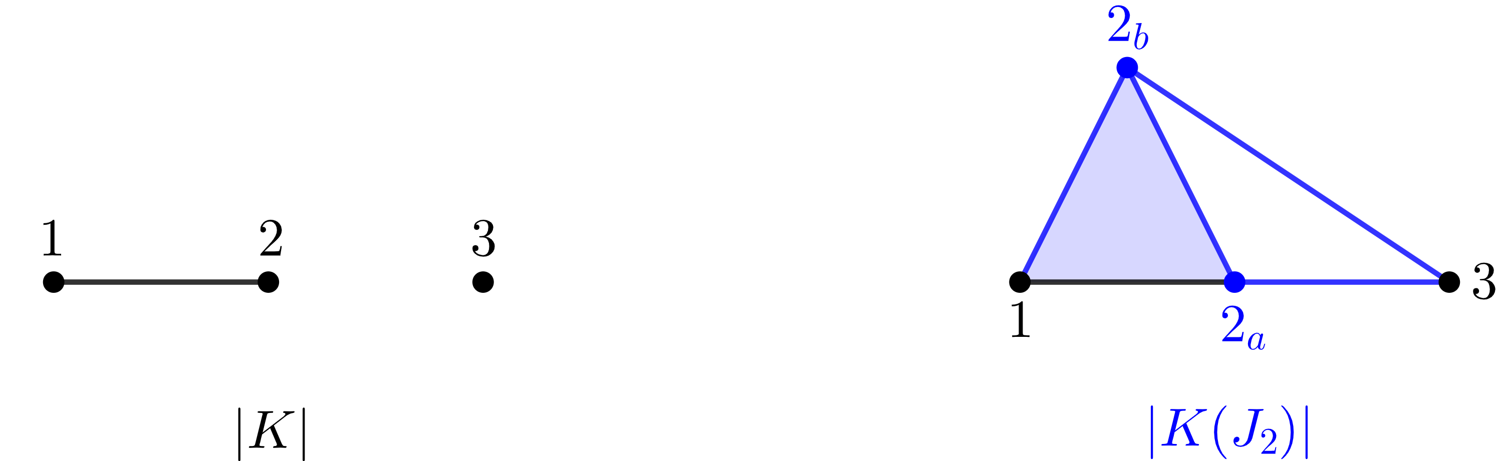
   Figure 6. $K(J_{2})=\{\{1,2_{a},2_{b}\},\{2_{a},3\},\{2_{b},3\},\text{their subsets}\}$.

2. For $m=3$, consider $K=\{\{1,2\},\{1,3\},\{2,3\},\text{their subsets}\}$ and $J=(2,1,1)$. We have

   $$\widehat{Z}(K;(\underline{D^{J+1}},\underline{S^{J}})) =\widehat{Z}(K;\{(D^{3},S^{2}),(D^{2},S^{1}),(D^{2},S^{1})\})$$

   $$\cong\widehat{Z}(K(J_{1});(\underline{D^{J^{\prime}+1}},\underline{S^{J^{\prime}}})),\ \text{where}\ J^{\prime}=(1,0,1,1).$$

   With $K(J_{1})=\{\{1_{a},1_{b},2\},\{1_{a},1_{b},3\},\{1_{a},2,3\},\{1_{b},2,3\},\text{their subsets}\}$, which is a simplicial complex with $m+1=4$ vertices.

The second intermediate result in given by the following lemma, which states that the geometric realization of the simplicial complex $K(J_{i})$ can be obtained just by considering a single suspension of the geometric realization of the simplicial complex $K$.

Lemma 6.5.

For any $i\in[m]$, we have

$$|K(J_{i})|\cong\Sigma|K|.$$

Proof.

Set $S^{0}=\{s_{1},s_{2}\}$ to be the $0$-sphere. We have

$$\Sigma|K| =S^{0}\ast|K|$$

$$=\{s_{1},s_{2}\}\ast\left(\bigcup_{\sigma\in K}|\sigma|\right)$$

$$=\bigcup_{\sigma\in K}\left(\{s_{1},s_{2}\}\ast|\sigma|\right)$$

$$=\left(\bigcup_{\sigma\in K,i\in\sigma}\left(\{s_{1},s_{2}\}\ast|\sigma|\right)\right)\cup\left(\bigcup_{\sigma\in K,i\notin\sigma}\left(\{s_{1},s_{2}\}\ast|\sigma|\right)\right)$$

$$\cong\left(\bigcup_{\sigma\in K,i\in\sigma}\left(|\sigma\backslash\{i\}\cup\{s_{1},s_{2}\}|\right)\right)\cup\left(\bigcup_{\sigma\in K,i\notin\sigma}\left(|\sigma\cup\{s_{1}\}|\cup|\sigma\cup\{s_{2}\}|\right)\right)$$

$$=\left(\bigcup_{\sigma\in K,i\in\sigma}\left(|\sigma\backslash\{i\}\cup\{s_{1},s_{2}\}|\right)\right)\cup\left(\bigcup_{\sigma\in K,i\notin\sigma}\left(|\sigma\cup\{s_{1}\}|\right)\right)\cup\left(\bigcup_{\sigma\in K,i\notin\sigma}\left(|\sigma\cup\{s_{2}\}|\right)\right)$$

$$\cong\left(\bigcup_{\sigma\in K,i\in\sigma}\left(|\sigma\backslash\{i\}\cup\{i_{a},i_{b}\}|\right)\right)\cup\left(\bigcup_{\sigma\in K,i\notin\sigma}\left(|\sigma\cup\{i_{a}\}|\right)\right)\cup\left(\bigcup_{\sigma\in K,i\notin\sigma}\left(|\sigma\cup\{i_{b}\}|\right)\right)$$

$$=\bigcup_{\tau\in K(J_{i})}|\tau|$$

$$=|K(J_{i})|.\qed$$

The lemma is illustrated in Figure 7 for the simplicial complex $K$ from Example 6.4(1).

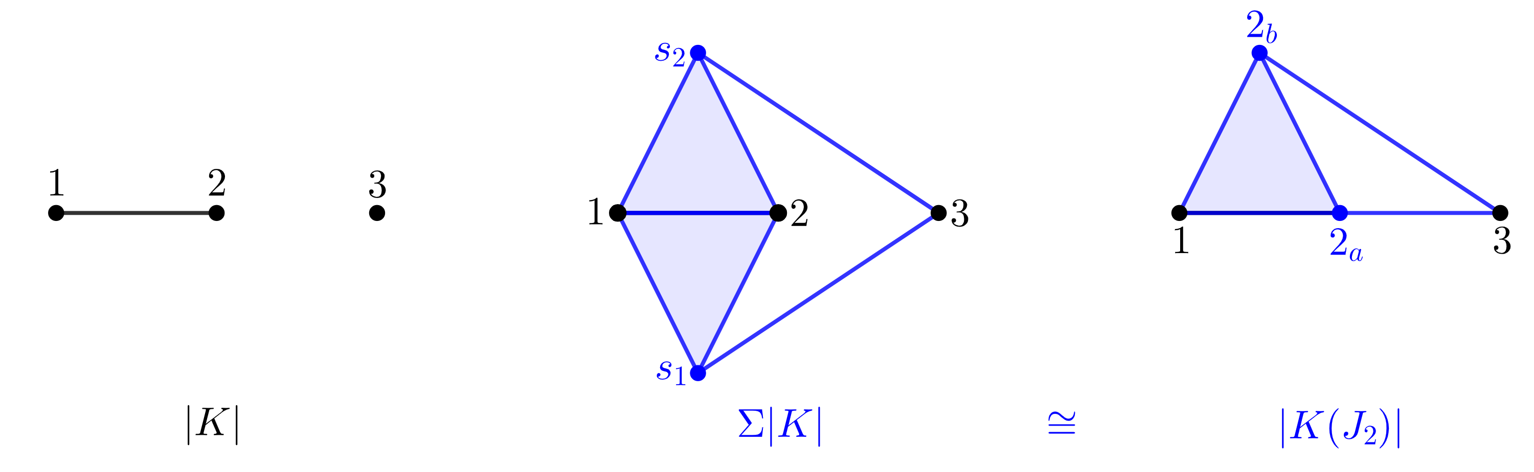
Figure 7. $|K(J_{2})|\cong\Sigma|K|$.

Now we can state and prove the main result.

Theorem 6.6.

For any $m$-tuple $J=(j_{1},\cdots,j_{m})$ in $({\mathbb{N}}\cup\{0\})^{m}$, there is a homeomorphism

$$\widehat{Z}(K;(\underline{D^{J+1}},\underline{S^{J}}))\cong\Sigma^{j_{1}+\cdots+j_{m}+1}|K|.$$

Proof.

Applying Lemma 6.3 $\sum_{i=1}^{m}j_{i}$ times, we get

(18) $$\widehat{Z}(K;(\underline{D^{J+1}},\underline{S^{J}}))\cong\widehat{Z}(K(J);(\underline{D^{1}},\underline{S^{0}})),$$

where $K(J)$ is a simplicial complex obtained by applying the basic move (doubling a single vertex) $\sum_{i=1}^{m}j_{i}$ times. By the base case $k=0$ in Theorem 5.1, we have

(19) $$\widehat{Z}(K(J);(\underline{D^{1}},\underline{S^{0}}))\cong\Sigma|K(J)|.$$

Finally, by applying Lemma 6.5 $\sum_{i=1}^{m}j_{i}$ times, we have

$$\Sigma|K(J)| \cong\Sigma\Sigma^{j_{1}+\cdots+j_{m}}|K|$$

(20) $$=\Sigma^{j_{1}+\cdots+j_{m}+1}|K|.$$

Therefore by putting equations $(\ref{gen1}),(\ref{gen2})$ and $(\ref{gen3})$ together, we obtain

$$\widehat{Z}(K;(\underline{D^{J+1}},\underline{S^{J}}))\cong\Sigma^{j_{1}+\cdots+j_{m}+1}|K|.\qed$$

References

- [1] A. Bahri, M. Bendersky, F. R. Cohen, and S. Gitler. The polyhedral product functor: a method of decomposition for moment-angle complexes, arrangements and related spaces. Adv. Math., 225(3):1634–1668, 2010.
- [2] A. Bahri, M. Bendersky, F. R. Cohen, and S. Gitler. Operations on polyhedral products and a new topological construction of infinite families of toric manifolds. Homology Homotopy Appl., 17(2):137–160, 2015.
- [3] V. M. Buchstaber and T. E. Panov. Toric topology, volume 204 of Mathematical Surveys and Monographs. American Mathematical Society, Providence, RI, 2015.
- [4] A. Hatcher. Algebraic topology. Cambridge University Press, Cambridge, 2002.
- [5] D. Stone. Private communication with A. Bahri. 2006.