Reliability and User-Plane Latency Analysis of mmWave Massive MIMO for Grant-Free URLLC Applications

Abstract

5G cellular networks are designed to support a new range of applications not supported by previous standards. Among these, ultra-reliable low-latency communication (URLLC) applications are arguably the most challenging. URLLC service requires the user equipment (UE) to be able to transmit its data under strict latency constraints with high reliability. To address these requirements, new technologies, such as mini-slots, semi-persistent scheduling and grant-free access were introduced in 5G standards. In this work, we formulate a spatiotemporal mathematical model to evaluate the user-plane latency and reliability performance of millimetre wave (mmWave) massive multiple-input multiple-output (MIMO) URLLC with reactive and $K$-repetition hybrid automatic repeat request (HARQ) protocols. We derive closed-form approximate expressions for the latent access failure probability and validate them using numerical simulations. The results show that, under certain conditions, mmWave massive MIMO can reduce the failure probability by a factor of $32$. Moreover, we identify that beyond a certain number of antennas there is no significant improvement in reliability. Finally, we conclude that mmWave massive MIMO alone is not enough to provide the performance guarantees required by the most stringent URLLC applications.

I Introduction

The 3rd generation partnership project (3GPP) has identified three distinct use cases for 5G new radio (NR) and beyond cellular networks based on their different connectivity requirements: enhanced mobile broadband (eMBB), massive machine-type communication (mMTC) and ultra reliable low-latency communication (URLLC) [1]. Since the inception of the idea of 5G NR, it has been argued that its main revolution is a change of paradigm from a smartphone-centric network to a network capable of satisfying the requirements of diverse services, such as machine-to-machine and vehicle-to-vehicle communications [2]. The URLLC scenario targets applications that require high reliability and low latency, such as augmented reality (AR), virtual reality (VR), vehicle-to-everything (V2X), critical internet of things (cIoT), industrial automation and healthcare. According to the use cases defined in [3], the main key performance indicator (KPI) to be satisfied in URLLC applications is the latent access failure probability, which incorporates the reliability and latency requirements needed in such applications. The requirements for URLLC applications vary from $1-10^{-5}$ transmission reliability to transmit $32$ bytes of data with a user-plane latency of less than $1$ ms to a $1-10^{-5}$ reliability to transmit $300$ bytes with a user-plane latency of between $3$ and $10$ ms, depending on the application [3].

lte and prior networks were not designed with such constraints in mind. Scheduling in long-term evolution (LTE) follows a grant-based approach, where the user equipment (UE) must request resources in a $4$-step random access (RA) procedure before transmitting data [4]. In the best-case scenario, it takes at least $10$ ms for a UE to start transmitting its payload.

Therefore, new mechanisms were introduced into the 5G NR specification to support the latency requirements of URLLC applications. Firstly, a flexible numerology was proposed, introducing the concept of a mini-slot that last as little as $0.125$ ms [5], in contrast to the $1$ ms minimum slot duration on LTE, enabling fine-grained scheduling of network resources [6]. Secondly, the introduction of semi-persistent scheduling (SPS) of grants [7, 8], where some of the networkś resource blocks are periodically reserved for URLLC applications, thereby avoiding the grant request procedure. Despite the efforts, not all URLLC applications have a periodic traffic pattern and are therefore unable to benefit greatly from SPS. Additionally, some services require low latency and reliable transmission to transmit small sporadic packets. With that in mind, both the standards committee [9] and researchers have put a lot of effort to investigate grant-free transmission, where the UEs transmit their payload directly in the RA channel. This culminated with the introduction of the $2$-step RA procedure introduced in Release 16 [9]. The $2$-step RA procedure follows a grant-free approach, where instead of waiting for a dedicated channel to be assigned by the network, it transmits its data directly into the RA channel and waits for feedback from the network [10].

Moreover, massive multiple input multiple output (MIMO) is a fundamental part of 5G NR [11, 12, 13]. It provides performance gains by improving diversity against fading and, along with advanced signal processing techniques, can provide directivity to transmission/reception, mitigating interference between spatially uncorrelated UEs [14]. The performance enhancements provided by MIMO are essential to ensure the reliability and the low latency required by URLLC applications. In conjunction with massive MIMO comes millimeter wave (mmWave) transmission. Due to its small wavelength, mmWave antennas can be packed into massive arrays, making it a key enabler of massive MIMO systems which attracted a significant interest on the topic [15, 16, 17, 18, 19, 20]. However, mmWave propagation comes with its own challenges due to the severe propagation loss experienced by electromagnetic signals in this frequency range.

In this paper, we develop a spatiotemporal analytical model to evaluate the performance of mmWave massive MIMO communication systems for URLLC applications. We use tools from stochastic geometry and probability theory to evaluate and compare system performance metrics by deriving closed-form approximate expressions for its latent access failure probability under different hybrid automatic repeat request (HARQ) protocols.

I-A Related Work

In [21], the authors propose a queueing model to compare the throughput performance of packet-based (grant-free) and connection-based (grant-based) random access. They conclude that packet-based systems with sensing can achieve greater throughput than connection-based one for small packet transmissions. In [22, 23], the optimization of grant-free access networks is investigated. The former considers the dynamic optimization of HARQ and scheduling parameters with non-orthogonal multiple access (NOMA), while the former considers the distributed link adaptation problem. Both papers formulate the respective optimization tasks as multiagent reinforcement learning (MARL) problems. The probability of success and the area spectral efficiency of a grant-free sparse code multiple access (SCMA) system is evaluated in [24, 25], in an mMTC context, using stochastic geometry. However, none of the works consider the temporal aspects of the system, which are crucial to analyze the latency and reliability of URLLC service. In [26], the probability of success of grant-free RA with massive MIMO in the sub-6 GHz band is investigated, and analytical expressions are derived for conjugate and zero-forcing beamforming. Despite its contribution, the authors do not evaluate the systemś temporal behavior, which is fundamental to characterize URLLC service’s performance. Moreover, due to its distinct propagation characteristics, this model is unsuitable for mmWave frequency bands.

The authors in [27] evaluate the scalability of scheduled uplink (grant-based) and random access (grant-free) transmissions in massive internet of things (IoT) networks, although they frame the problem through a revolutionary spatiotemporal framework, fusing stochastic geometry and queueing theory. They conclude that grant-free transmission offers lower latency, however, it does not scale well to a massive number of devices. In our work, we show that using massive MIMO base stations is a viable solution to address the scalability issues of grant-free transmission without sacrificing its latency, rendering it particularly suitable for URLLC applications. In [28], the authors use a similar spatiotemporal model to characterize the performance of different RA schemes with respect to the probability of a successful preamble transmission in a grant-based massive IoT system. They conclude that a backoff scheme performs close to optimally in diverse traffic conditions. In [29], the authors perform system-level simulations of a grant-free URLLC network under different HARQ configurations, and compare it to a baseline grant-based system. They conclude that grant-free systems provide significantly lower latency at the $1-10^{-5}$ reliability level. The same scenario is evaluated in [30], however, the authors characterize system performance analytically, using a stochastic geometry-based spatiotemporal model. This paper identifies the suitability of each HARQ scheme for different network loads and received power levels.

Stochastic geometry has become the de facto tool for analyzing large networks [31, 32, 33], and has been successfully used to investigate the performance of MIMO systems for a while now [34, 35, 36, 37]. In [38], a unified stochastic geometric mathematical model for MIMO cellular networks with retransmission is proposed. In [39], a stochastic geometry-based analytical model for the performance of downlink mmWave NOMA systems is developed. The authors propose two random beamforming methods that are able to reduce system overhead while providing performance gains for BSs with a large number of antennas.

We seek to answer the following main questions that are to the best of our knowledge missing from the current literature:

• How do we formulate a tractable spatiotemporal model to investigate the reliability and latency of URLLC applications powered by BSs equipped with massive antenna arrays operating on mmWave frequencies?

• What closed-form analytical expressions can we derive for the latent access failure probability in this scenario?

• What are the performance gains obtained from increasing the number of antennas at the BS, and what are the limitations?

I-B Contributions

This paper makes three major contributions:

• We formulate a mathematical model to evaluate the performance of mmWave massive MIMO on uplink grant-free URLLC networks with HARQ. This model uses stochastic geometry to capture the spatial configuration of the UEs and the BSs, a mmWave channel model, and probability theory to obtain the temporal characteristics necessary to evaluate the performance of URLLC applications.

• We derive closed-form approximate expressions for the latent access failure probability using reactive and $K$-repetition HARQ schemes. To the best of our knowledge, no previous works has presented closed-form analytic expressions for this key performance measure of URLLC applications in a mmWave massive MIMO communication system.

• We analyze the system performance for an extensive range of scenarios, identifying the gains and limitations provided by using the mmWave spectrum together with a massive number of antennas at the BS, and identify the scenarios that benefit the most from these two technologies.

I-C Notation and Organization

Italic Roman and Greek letters denote deterministic and random variables, while bold letters denote deterministic and random vectors. The capital Greek letter $\Phi$ denotes a point process and $x\in\Phi$ represents a point belonging to said process. The notation $\Phi(A)$, where $A\in\mathbb{R}^{d}$, is the counting process associated with $\Phi$ [40]. Notice that we overload the meaning of $\Phi$ so that it can signify a point process, a counting measure or a set depending on the context. ${n\choose k}=\frac{n!}{k!\left(n-k\right)!}$ is the binomial coefficient of $n$ choose $k$.

The uniform, complex normal and binomial distributions are represented by $Uniform(a,b)$, $\mathcal{CN}(\mu,\sigma^{2})$ and $Binomial(p)$, respectively. The vector $\mathbf{x}^{H}$ is the Hermitian transpose of vector $\mathbf{x}$. The function $\mathbb{P}(\cdot)$ denotes the probability of the event within parentheses. The notation $\mathbf{1}\left\{\cdot\right\}$ denotes the indicator function, which is equal to one whenever the event within curly braces is true and zero otherwise.

This work is divided into five sections and an appendix. In Section I, we introduce the contents of the manuscript and contextualize within the relevant literature. In Section II, we present a mathematical model to characterize the performance of the grant-free mmWave massive MIMO system in URLLC applications. In Section III, we derive the latent access failure probability of the proposed system using reactive and $K$-repetition HARQ protocols. In Section IV, we show the results of the system simulation. We use these results to validate the analytical derivations, investigate the system’s performance for an extensive range of parameters and finish it by interpreting the results in the context of URLLC applications. In Section V, we summarize our findings and present our conclusions. Finally, in the appendix, we show the detailed proofs of the lemmas and theorems required by the derivations in the paper.

II System Model

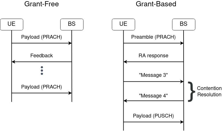
Figure 1: Comparison of the transmission procedure in grant-free and grant-based systems.

In most cellular applications, uplink transmissions use a dedicated resource (frequency, time or a MIMO spatial layer) previously assigned by the network to transmit their data payload. Thus, when an UE receives new data, it must send a request for the network to schedule a resource. With dedicated resources, each UE can utilize the wireless channel to its full capacity, thus maintaining good quality of service (QoS). TIn 5G NR networks, the schedule request consists of four steps, illustrated in Figure 1:

• The UE randomly selects one of the available preambles and transmits it on the physical random access channel (PRACH).

• The BS transmits a random access request (RAR), acknowledging receipt of the preamble and time-alignment commands.

• The UE and BS exchange contention resolution messages (messages 3 and 4) that are used to identify possible collisions arising from two different devices transmitting the same preamble.

• If the grant request is successful, the UE transmits its payload on the physical uplink shared channel (PUSCH).

This grant-based scheme is efficient for applications that need to use the channel multiple times to transmit large amounts of data (e.g., video streaming) or data that’s being continuously generated (e.g., voice). However, in some URLLC applications, UEs sporadically generate data that need to be transmitted reliably and with low latency, such as cIoT and sensors for industrial automation. In such scenarios, the time spent on the schedule request renders grant-based schemes inefficient. A more suitable alternative is to transmit the data directly on the PRACH and thereby avoidall the overhead involved in requesting a grant, as illustrated in Fig. 1. Nonetheless, with grant-free transmission comes the possibility of collisions whenever two UEs randomly select the same preambles. Therefore, HARQ is used to ensure the reliability and robustness of grant-free transmission. harq consists of using feedback information from the BS so the UE can retransmit packets that were not successfully received. Despite this, it can be quite challenging to scale grant-free networks because wireless resources are finite and expensive. To this end, massive MIMO and beamforming can be applied to reduce the interference of spatially uncorrelated UEs and thereby increasing the reliability of the system.

In this section, we discuss the spatial model of the network, the mmWave channel model, the BS receiver beamforming procedure and the different HARQ schemes used.

II-A Physical Layer Model

Stochastic geometry and the theory of random point processes has proven to be able to accurately model the spatial distribution of modern cellular network deployments [41]. Therefore, we consider a cell of radius $R$ consisting of a BS, equipped with $K$ antennas, located at the origin. We model the spatial location of the single-antenna UEs according to a homogeneous Poisson point process (HPPP) [40], denoted by $\Phi_{U}$ with intensity $\lambda_{U}$. Furthermore, the distance between the $i$-th UE, $x_{i}\in\Phi_{U}$, and the BS is given by $\left\lVert x_{i}\right\rVert$. Both the distance from the UE to the BS and its normalized angle from the BS are uniformly distributed random variables [40], $\left\lVert x_{i}\right\rVert\sim Uniform(0,R)$ and $\theta_{i}\sim Uniform(-1,1)$, respectively.

Due to path loss attenuation, the signal received from UEs located further from the BS is “drowned” by the signal from closer users transmitting with the same power, also known as the near-far problem. Uplink power control is fundamental to deal with this issue. We consider that the UEs utilize path loss inversion power control [42], with received power threshold $\rho$, where each user controls its transmit power such that the average received power at its associated BS is $\rho$, by selecting their transmit powers as $p_{i}=\rho\left\lVert x_{i}\right\rVert^{\alpha}$, where $\alpha$ is the path loss exponent. We assume that there are $N_{S}$ subcarriers reserved for grant-free URLLC transmissions and $N_{P}$ orthogonal preambles. Thus, at each transmission time interval (TTI), the active UEs select a subcarrier and preamble randomly from the $N_{S}$ available subcarriers and $N_{P}$ available preambles. Moreover, we assume that at $t=0$, one packet arrives to the transmitting queue of each UE. Therefore, the HPPP of active users $\Phi_{A}$ on a specific subcarrier is obtained by thinning $\Phi_{U}$ [40] and its effective intensity at $t=0$ is given by

$$\lambda_{A}=\frac{\lambda_{U}}{N_{S}}.$$ (1)

Massive MIMO technology and mmWave frequencies are intrinsically connected. Even though one does not imply the other, they complement each other really well. The former requires large antenna arrays, and the size of such arrays is proportional to the targeted wavelength. Moreover, mmWave antennas must be really small to operate in such large frequencies, therefore, a larger number of them are necessary to gather enough energy. In this work, we consider that the BS is equipped with a massive uniform linear array (ULA) containing $K\gg 1$ antennas operating at mmWave frequencies, while the UEs possess a single antenna. The channel vector between user $i$ and the bs is given by

$$\mathbf{h}_{i}=\sqrt{K}\left[\underbrace{\frac{g_{i,0}\mathbf{a}(\theta_{i}^{0})}{\sqrt{\left\lVert x_{i}\right\rVert^{\alpha_{LOS}}}}}_{\text{LOS component}}+\underbrace{\frac{\underset{j=1}{\overset{J}{\sum}}g_{i,j}\mathbf{a}(\theta_{i}^{j})}{\sqrt{\left\lVert x_{i}\right\rVert^{\alpha_{NLOS}}}}}_{\text{NLOS components}}\right],$$ (2)

where $g_{i,j}\sim\mathcal{CN}(0,1)$ is the complex gain on the $j$-th path and $\theta^{j}_{i}$ is the normalized direction of the $j$-th path. We assume that the complex gains of different paths are independent. $\alpha_{LOS}$ and $\alpha_{NLOS}$ denote the path loss exponent of the line-of-sight (LOS) and non-line-of-sight (NLOS) paths, respectively. The vector

$$\mathbf{a}(\theta)=\frac{1}{\sqrt{K}}\begin{bmatrix}1&e^{-j\pi\theta}&\dots&e^{-j\pi(K-1)\theta}\end{bmatrix}^{T}$$ (3)

denotes the phase of the signal received by each antenna. Due to high penetration losses suffered by mmWave signals, the LOS path has a dominant effect on channel gain, being $20$ dB larger than the NLOS in some cases [39, 37]. Hence, we can safely approximate $\mathbf{h}_{i}$ as

$$\mathbf{h}_{i}\approx\sqrt{K}\frac{g_{i}\mathbf{a}(\theta_{i})}{\sqrt{\left\lVert x_{i}\right\rVert^{\alpha}}}$$ (4)

for mathematical tractability. Additionally, to avoid cluttering the notation, we drop the subscripts denoting different paths and distinguishing LOS and NLOS variables.

Due to the dominant effect of the LOS link, the channel model also needs to consider a blockage model to determine the probability that the LOS path between the UE the BS is obstructed. To model the effects of blockage, we adopt the model proposed in [43]. This model is obtained by assuming that the obstructing building and structures form an HPPP with random width, length and orientation. So, let $LOS$ be the set of los UEs; then, the probability that user $x_{i}$ has a LOS link is given by

$$\mathbb{P}\left(x_{i}\in LOS\right)=\exp\left(-\beta\left\lVert x_{i}\right\rVert\right),$$ (5)

where $\beta$ is directly proportional to the density, and the average width and length of obstructing structures. This model nicely captures the exponentially vanishing probability of having a LOS link the further you move away from the BS, and can be easily fitted to real urban scenarios.

Signal Model

At each TTI, the active users transmit an information signal $s_{i}$ such that $\left\lvert s_{i}\right\rvert=1$. Therefore, the vector of the signal received at the BS is given by

$$\mathbf{y}=\underset{x_{i}\in\Phi_{A}}{\sum}\mathbf{1}\left\{x_{i}\in LOS\right\}\sqrt{\rho}\mathbf{h}_{i}s_{i}+\mathbf{n},$$ (6)

where $\mathbf{n}\sim\mathcal{CN}\left(0,\sigma_{2}\mathbf{I}\right)$ is a circularly symmetric complex Gaussian random variable representing additive white Gaussian noise (AWGN).

To successfully recover the data transmitted by a given user, the BS must be able to accurately estimate its channel response.

Definition 1 (Preamble Collision).

Preamble collision event, denoted by $C$, happens when two or more devices transmit the same preamble on the same subcarrier.

We assume that the BS is able to perfectly estimate the UE channel response $\mathbf{h}_{i}$ whenever there is no preamble collision. Then, the BS performs conjugate beamforming to separate the intended user’s signal from those of the other interfering UEs by multiplying the received signal by the Hermitian transpose of the intended user channel response. Therefore the recovered signal of the intended user, the $j$-th user, is

$$y_{j} = \mathbf{1}\left\{x_{j}\in LOS\right\}\mathbf{1}\left\{\bar{C}\right\}\sqrt{\rho}\mathbf{h}_{j}^{H}\mathbf{h}_{j}s_{j}+$$

$$\underset{x_{i}\in\Phi_{A}\setminus\left\{x_{j}\right\}}{\sum}\mathbf{1}\left\{x_{i}\in LOS\right\}\sqrt{\rho}\mathbf{h}_{j}^{H}\mathbf{h}_{i}s_{i}+\tilde{n}_{j},$$

where $\bar{C}$ is the event when user $j$ does not experience preamble collision and $\tilde{n}_{j}\sim\mathcal{CN}\left(0,\sigma^{2}\right)$ is a linear combination of the noise vector, which is a Gaussian distributed random variable. Therefore, the signal-to-interference-plus-noise-ratio (SINR) experienced by user $j$ is given by

$$\mathrm{SINR}$$ (8)

$$= \frac{\mathbf{1}\left\{x_{j}\in LOS\cap\bar{C}\right\}\rho\left\lvert\mathbf{h}_{j}^{H}\mathbf{h}_{j}\right\rvert^{2}}{\underset{x_{i}\in\Phi_{A}\setminus\left\{x_{j}\right\}}{\sum}\mathbf{1}\left\{x_{i}\in LOS\right\}\rho\left\lvert\mathbf{h}_{j}^{H}\mathbf{h}_{i}\right\rvert^{2}+\sigma^{2}}$$

$$= \frac{\mathbf{1}\left\{TX_{j}\right\}\rho\left\lvert g_{j}\right\rvert^{2}\left\lvert\mathbf{a}\left(\theta_{j}\right)^{H}\mathbf{a}\left(\theta_{i}\right)\right\rvert^{2}}{I+\sigma^{2}},$$

where $TX_{j}=\{x_{j}\in LOS\cap\bar{C}\}$ is the probability that user $j$ has a LOS link and does not suffer from preamble collision, and $I=\underset{x_{i}\in\Phi_{A}\setminus\left\{x_{j}\right\}}{\sum}\mathbf{1}\left\{x_{i}\in LOS\right\}\rho\left\lvert g_{i}\right\rvert^{2}\left\lvert\mathbf{a}\left(\theta_{j}\right)^{H}\mathbf{a}\left(\theta_{i}\right)\right\rvert^{2}$ is the interference from the other UEs. Moreover, the beamforming gain, $\left\lvert\mathbf{a}\left(\theta_{j}\right)^{H}\mathbf{a}\left(\theta_{i}\right)\right\rvert^{2}$, can be expressed as [44]

$$\begin{split}\left\lvert\mathbf{a}\left(\theta_{j}\right)^{H}\mathbf{a}\left(\theta_{i}\right)\right\rvert^{2}&=F_{K}\left(\frac{\pi}{2}\left(\theta_{i}-\theta_{j}\right)\right)\\ &=\frac{1}{K}\left\lvert\frac{\sin\left(\frac{K\pi}{2}\left(\theta_{i}-\theta_{j}\right)\right)}{\sin\left(\frac{\pi}{2}\left(\theta_{i}-\theta_{j}\right)\right)}\right\rvert^{2},\end{split}$$ (9)

where $F_{K}(x)$ is the Fejer kernel [45], with $F_{K}(0)=K$.

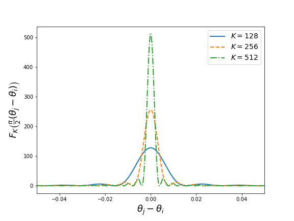
Figure 2: Fejer kernel value for normalized angles of arrival varying from $-0.2$ to $0.2$.

A useful property of the Fejer kernel is that [45]

$$\underset{K\rightarrow\infty}{\lim}\int_{\delta\leq\left\lvert x\right\rvert\leq\pi}F_{K}(x)dx=0,$$ (10)

meaning that for an asymptotically large value of $K$, the interference for the signals not aligned with beam angle $\theta_{j}$ goes to zero. Fig. 2 illustrates this property by plotting the Fejer kernel for increasing values of $K$.

II-B HARQ Schemes

HARQ protocols determine how transmitters and receivers exchange information about successful packet reception, by transmitting an acknowledgement (ACK) signal, and how UEs retransmit in the event of failure, which is signaled by the transmission of a negative acknowledgement (NACK) signal. They are especially important to ensure reliability in grant-free transmission. The HARQ protocol used also impacts the overall latency of the system. Hence, in this paper, we investigate the performance of the massive MIMO URLLC network under two distinct HARQ protocols.

With respect to transmissions latency, the HARQ protocols investigated have a few aspects in common. First, the UE spends $T_{A}$ TTIs to process a newly arrived packet. As soon as the packet is processed, it spends $T_{TX}$ TTIs transmitting it. Upon receipt of the packet, the BS spends $T_{DP}$ TTIs to process it and $T_{F}$ TTIs to send feedback and for it to reach the UE. Once the UE receives the feedback signal, it takes $T_{UP}$ TTIs to process it. We consider that the transmit and feedback time already take into account the propagation delay between the transmitter and receiver. Without loss of generality, we assume that $T_{A}=T_{TX}=T_{DP}=T_{UP}=1$ TTI. Another concept shared between different HARQ protocols is the round-trip time (RTT), which consists of the time it takes from the start of a transmission by the UE to the end of processing of the feedback signal, either ACK or NACK, the UE received from the BS.

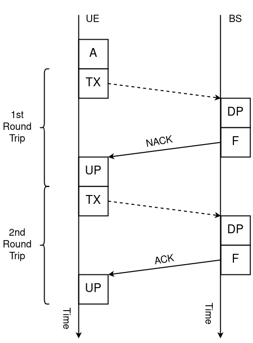
Figure 3: An illustration of a couple of reactive HARQ protocol round trips.

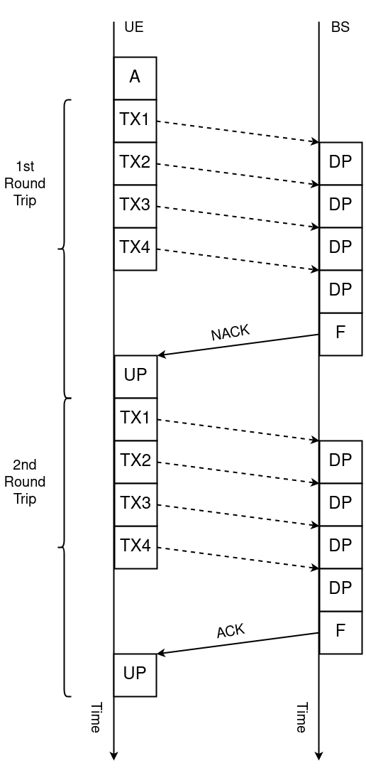
Figure 4: An illustration of a couple of $K$-repetition HARQ protocol round trips.

II-B1 Reactive Scheme

The reactive HARQ protocol is the more straight-forward one of the two considered in this paper. The UE attempts to transmit one packet and waits for feedback from the BS. Once the feedback is processed, it either attempts to retransmit the same packet if it got a NACK signal or sits idle until a new packet arrives. This protocol is illustrated in Fig. 3, which shows the processing times and signal exchange between the UE and the BS. Under the assumptions considered in this paper, the reactive RTT $T^{reac}_{RTT}$ is given by

$$T^{reac}_{RTT}=4\text{ TTIs}.$$ (11)

From (11), the user-plane latency of the $m$-th HARQ round-trip is

$$T^{reac}(m)=T_{A}+4m\text{ TTIs}.$$ (12)

II-B2 $K$-Repetition Scheme

To increase the reliability and robustness of each transmission attempt, the $K$-repetition HARQ protocol repeats the same packet $K_{rep}$ times on each attempt. Therefore, the only way a transmission attempt fails is if each of the $K_{rep}$ transmissions fail, which translates into an increased reliability of the overall system. However, feedback on the transmission attempt is sent only after the last repetition is processed by the BS. So, there is a tradeoff between enhancing the reliability of each transmission and increasing the latency of a transmition attempt. Fig. 4 shows two $K$-repetition round-trip transmissions, where the first transmission fails and the second is successful. The RTT of the $K$-repetition HARQ protocol is

$$T^{K_{rep}}_{RTT}=K_{rep}+3\text{ TTIs}.$$ (13)

Therefore, the total latency of $m$ $K$-repetition transmissions is given by

$$T^{K_{rep}}(m)=T_{A}+mT^{K_{rep}}_{RTT}=1+m(K_{rep}+3)\text{ TTIs}.$$ (14)

III System Analysis

The main requirement of URLLC applications is to reliably keep the user-plane latency below an application-dependent latency constraint. We begin this section by unambiguously defining what we mean by reliably and user-plane latency.

Definition 2 (User-Plane Latency).

User-plane latency is the time spent between the arrival of a packet to the UE’s queue and the successful processing of an ACK signal received from the BS.

Definition 3 (Latent Access Failure Probability Requirement).

Latent access failure probability $\mathcal{P}_{F}(T\leq\tau)$, where $T$ is the user-plane latency and $\tau$ is the latency constraint, is the probability that the UE data cannot be successfully decoded.

Therefore, the QoS requirement of URLLC applications can be stated as

$$\mathcal{P}_{F}(T\leq\tau)\leq\epsilon,$$ (15)

where $\tau$ is the latency constraint and $\epsilon$ is the minimum reliability, and both are application-dependent. Thus, to satisfy the QoS requirement, the probability that an UE cannot transmit its data before $\tau$ must be bounded by $\epsilon$. Typically, $\tau$ varies between $1$ and $10$ ms and $\epsilon$ varies between $10^{-5}$ and $10^{-6}$ depending on the URLLC application.

Let $M$ be the maximum number of retransmissions under the latency constraint $\tau$. Moreover, notice that some of the UEs will transmit successfully earlier than others, and if the UE’s transmission queue stays idle, the interference levels in distinct retransmissions are different. Therefore, the latent access failure probability is a function of the fraction of active users at the $m$-th retransmission ($\mathcal{A}_{m}$), the probability that the $m$-th retransmission is successful ($\mathcal{P}_{m}$( and the maximum number of retransmissions ($M$), as given by [30]

$$\mathcal{P}_{F}(T\leq\tau)=\begin{cases}1,&\text{, if }M=0\\ 1-\underset{m=1}{\overset{M}{\sum}}\mathcal{A}_{m}\mathcal{P}_{m}&\text{, if }M\geq 1,\end{cases}$$ (16)

where $\mathcal{A}_{m}$ is

$$\mathcal{A}_{m}=\begin{cases}1,&\text{, if }m=1\\ 1-\underset{i=1}{\overset{m-1}{\sum}}\mathcal{A}_{i}\mathcal{P}_{i}&\text{, if }m\geq 2.\end{cases}$$ (17)

Given the expressions for $\mathcal{P}_{m}$, the latent access failure probability is obtained by iteratively computing (17) and (16).

In the rest of this section, we derive closed-form expressions for $\mathcal{P}_{m}$ under the reactive and $K$-repetition HARQ protocols, denoted by $\mathcal{P}^{reac}_{m}$ and $\mathcal{P}^{Krep}_{m}$, respectively. To do so, we use stochastic geometric analysis to obtain the probability of success of a randomly chosen user $x_{0}$, herein the typical user. From Slivnyak’s theorem [46], the performance of the typical user in an HPPP is representative of the average user’s performance.

III-A Reactive HARQ

The maximum number of HARQ transmissions following the reactive HARQ protocol with the delay constraint $\tau$ is given by

$$M^{reac}=\left\lceil\frac{\tau-1}{T^{reac}_{RTT}}\right\rceil=\left\lceil\frac{\tau-1}{4}\right\rceil.$$ (18)

The first step in deriving an expression for the latent access failure probability is to obtain the probability that the $m$-th reactive retransmission is successful ($\mathcal{P}^{reac}_{m}$).

Let $\Phi_{I}=\{x_{i}\lvert x_{i}\in\Phi_{A}\setminus\left\{x_{0}\right\}\cap x_{i}\in LOS_{m}\}$ be the set of users interfering with the typical user’s transmission on the $m$-th RTT. Notice that due to the exponentially decreasing probability of a LOS link with the increase in distance, $\Phi_{I}$ is a non-HPPP with density $\lambda_{I}(x)=\lambda_{A}\exp\left(-\beta\left\lVert x\right\rVert\right)$. The mean measure of $\Phi_{I}$, the average number of points in a given area, is obtained as

$$\Lambda\left(b(0,r)\right) = E\left[\Phi_{I}\left(b(0,r)\right)\right]=\int_{\mathbb{R}^{2}}\lambda_{I}(x)dx$$

$$= 2\pi\lambda_{A}\int_{0}^{r}\exp\left(-\beta r\right)rdrd\theta$$

$$= \frac{2\pi\lambda_{A}}{\beta^{2}}\left[1-\exp\left(-\beta r\right)\left(1+\beta r\right)\right],$$

where $b(0,r)$ is a $2$-dimensional ball with radius $r$ that is centered at the origin. Now, let $N_{m}$ be a random variable denoting the number of users that interfere with the typical user on the $m$-th retransmission. From (III-A), the probability that there are $n$ interferers in the cell with radius R is derived as

$$\mathbb{P}\left(N_{m}=n\right) = \frac{\left[\mathcal{A}^{reac}_{m}\Lambda\left(b(0,R)\right)\right]^{n}}{n!}$$

$$\times\exp\left(-\mathcal{A}^{reac}_{m}\Lambda\left(b(0,R)\right)\right).$$

Lemma 1.

If $K\gg 1$, the probability that the $m$-th reactive HARQ retransmission of the typical user conditioned on the events that the typical user does not experience preamble collision, has a LOS link and is affected by $n$ interferers can be approximated as

$$\mathbb{P}\left(\mathrm{SINR}_{m}\geq\gamma\left\lvert TX_{0},N_{m}=n\right.\right)$$

$$\approx \underset{n^{\prime}=0}{\overset{n}{\sum}}{n\choose n^{\prime}}\left(\frac{2}{K}\right)^{n^{\prime}}\left(1-\frac{2}{K}\right)^{n-n^{\prime}}$$

$$\times\exp\left(-\frac{\gamma}{\rho K}\right)\left[\frac{\tanh^{-1}\left(\sqrt{\frac{\gamma}{1+\gamma}}\right)}{\sqrt{\gamma\left(1+\gamma\right)}}\right]^{n^{\prime}},$$

where $n^{\prime}$ is the number of interferers within the primary lobe of the beam directed at the typical user.

Proof.

See Appendix A. ∎

After deriving the expressions for the probability of having $N_{m}$ users interfere with retransmission $m$ in (III-A) and the conditional probability of success obtained in Lemma 1, the success probability can be obtained as follows:

Theorem 1.

The probability that the $m$-th reactive harq retransmission is successfully decoded is

$$\mathcal{P}_{m}^{reac}$$

$$= \underset{n=0}{\overset{\infty}{\sum}} \mathbb{P}(N_{m}=n)\mathbb{P}\left(\left.\bar{C}\right.\lvert N_{m}=n\right)$$

$$\times\mathbb{P}(x_{0}\in LOS_{m})$$

$$\times\mathbb{P} (\mathrm{SINR}_{m}\geq\gamma\left\lvert TX_{0},N_{m}=n\right.),$$

where $\mathbb{P}(N_{m}=n)$ is the probability that there are $n$ interferers in the cell and is given by (III-A). The probability of no preamble collision is given by

$$\mathbb{P}\left(\left.\bar{C}\right\lvert N_{m}=n\right)=\left(1-\frac{1}{Ns}\right)^{n}.$$ (23)

And finally, the probability that the typical user has a LOS link to the BS is

$$\mathbb{P}\left(x_{i}\in LOS_{m}\right) = \frac{1}{R}\int_{0}^{R}\exp\left(-\beta\left\lVert x_{i}\right\rVert\right)d\left\lVert x_{i}\right\rVert$$ (24)

$$= \frac{1}{\beta R}\left[1-\exp\left(-\beta R\right)\right].$$

Proof.

The proof is straight forward if the conditional probability obtained in Lemma 1 is averaged out. ∎

From the results of Theorem 1, the latent access failure probability can be easily obtained by iteratively computing

$$\mathcal{P}_{F}(T\leq\tau)=\begin{cases}1\text{, if }M^{reac}=0\\ 1-\underset{m=1}{\overset{M^{reac}}{\sum}}\mathcal{A}^{reac}_{m}\mathcal{P}^{reac}_{m}\text{,if }M^{reac}\geq 1.\end{cases}$$ (25)

III-B $K$-Repetition HARQ

In the $K$-repetition HARQ system, the RTT lasts from when the UE transmits the first repetition until it receives the ACK/NACK feedback signal. Thus, under delay constraint $\tau$, the maximum number of retransmissions is

$$M^{K_{rep}}=\left\lceil\frac{\tau-1}{T^{K_{rep}}_{RTT}}\right\rceil=\left\lceil\frac{\tau-1}{K_{rep}+3}\right\rceil.$$ (26)

Under the $K$-repetition HARQ, the same data is repeated $K_{rep}$ times for every transmission attempt, and after the BS receives all the repetitions, it sends either an ACK or a NACK signal depending whether any of the repetitions sent in the transmission could be successfully decoded. Additionally, the UE selects a new random subcarrier and preamble for the transmission of each distinct repetition. To obtain a closed-form expression for the latent access failure probability, we follow the same steps as were taken for the reactive HARQ derivation.

Lemma 2.

If $K\gg 1$, the probability that the $m$-th $K$-repetition HARQ retransmission of the typical user, conditioned on the event that the typical user does not experience preamble collision, has a LOS link and is affected by $n$ interferers can be approximated as (2), shown at the top of next page,

$$\mathbb{P}\left(\underset{l=1}{\overset{K_{rep}}{\bigcup}}\mathrm{SINR}_{m,l}\geq\gamma\left\lvert\bar{C},x_{0}\in LOS_{m},N_{m}=n\right.\right)\quad$$

$$\approx\underset{l=1}{\overset{K_{rep}}{\sum}}{K_{rep}\choose l}\left(-1\right)^{l+1}\underset{n^{\prime}=0}{\overset{n}{\sum}}{n\choose n^{\prime}}\left(\frac{2}{K}\right)^{n^{\prime}}\left(1-\frac{2}{K}\right)^{n-n^{\prime}}$$

$$\exp\left(-\frac{l\gamma}{\rho K}\right)\left[\frac{\tanh^{-1}\left(\sqrt{\frac{\gamma}{1+\gamma}}\right)}{\sqrt{\gamma\left(1+\gamma\right)}}\right]^{ln^{\prime}}$$ (27)

where the double subscript $m,l$ indicates the $l$-th repetition of the $m$-th HARQ retransmission attempt.

Proof.

See Appendix B. ∎

With the result from Lemma 2, the probability that the $m$-th retransmission attempt is successful can be obtained by averaging (2) over the conditional random variables.

Theorem 2.

The probability that the $m$-th $K$-repetition harq retransmission is successfully decoded is given by (28), shown at the top of next page,

$$\mathcal{P}_{m}^{K_{rep}}= \underset{n=0}{\overset{\infty}{\sum}} \mathbb{P}(N_{m}=n)\mathbb{P}\left(\left.\bar{C}\right.\lvert N_{m}=n\right)$$ (28)

$$\mathbb{P}(x_{0}\in LOS)\mathbb{P}\left(\underset{l=1}{\overset{K_{rep}}{\bigcup}}\mathrm{SINR}_{m,l}\geq\gamma\left\lvert\bar{C},x_{0}\in LOS_{m},N_{m}=n\right.\right),$$

where the closed-form expression for $\mathbb{P}\left(\underset{l=1}{\overset{K_{rep}}{\bigcup}}\mathrm{SINR}_{m,l}\geq\gamma\left\lvert\bar{C},x_{0}\in LOS_{m},N_{m}=n\right.\right)$ is derived on Lemma 2.

Given the analytical expression for the probability that the $m$-th $K$-repetition HARQ retransmission is successfully received by the BS in Theorem 2 and the fact that the probability that a randomly selected UE is active can be computed from (17), the latent access failure probability is derived as

$$\mathcal{P}_{F}(T\leq\tau)=\begin{cases}1,\text{, if }M^{K_{rep}}=0\\ 1-\underset{m=1}{\overset{M^{K_{rep}}}{\sum}}\mathcal{A}^{K_{rep}}_{m}\mathcal{P}^{K_{rep}}_{m}\text{,}\\ \text{if }M^{K_{rep}}\geq 1.\end{cases}$$ (29)

IV Numerical Results and Discussion

In this section, we report the results of Monte-Carlo simulations of the system model described in Section II. We use the simulation results to: a) validate the closed-form analytical approximations derived in Section III b) characterize the performance of the two HARQ protocols in the mmWave massive MIMO scenario and c) discuss the insights provided by the analytical results.

At the beginning of each simulation instance, the users’ locations are generated according to an HPPP inside a cell with radius $R=0.5$ km. At every TTI:

• The channel gain between the UEs and the BS located at the origin is generated as an exponential random variable with unit mean.

• All active UEs are determined to have either a LOS or NLOS link according to the probability in (24), with $\beta=1$.

• All active UEs select a random subcarrier from one of the $N_{S}=48$ subcarriers available.

• All active UEs select a random preamble from one of the $N_{P}=64$ preambles available.

• The BS checks all UEs with LOS links on every subcarrier for preamble collision.

• The BS computes the dot product between the signal received and the conjugate beam for all the UEs whose preambles have not collided. If the resulting SINR is greater than $\gamma=-2$ dB, the transmission is successful, otherwise it fails.

• The BS sends an ACK feedback signal to the UEs whose transmission was successful and a NACK feedback signal to those whose transmission attempt failed. As the main goal of this work is to characterize grant-free uplink performance, we assume that the feedback sent through the downlink channel is error free.

• All UEs move to a new location.

In accordance with 3GPP standards [47, 48], we consider a TTI mini-slot having a duration of $0.125$ ms and a subcarrier spacing of $60$ kHz, which is a configuration compatible with 5G NR frequency range 2 (FR2) operation, located in the mmWave spectrum. We consider a noise figure of $-174$ dBm/Hz, a path loss exponent of $\alpha=4$ and a received power threshold of $\rho=-130dBm$.

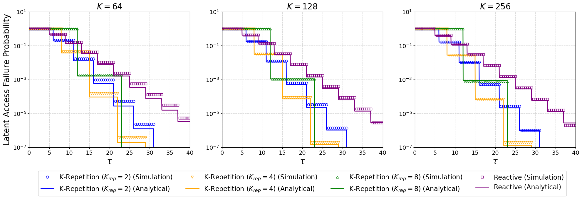
Figure 5: CCDF of the latent access failure probability for $\lambda_{U}=1000$ UE/$\text{km}^{2}$ for the reactive and $K$-repetition HARQ protocols with $K_{rep}=2,4,8$. The plots in the figure show the results for $K=64$, $K=128$ and $K=256$ antennas.

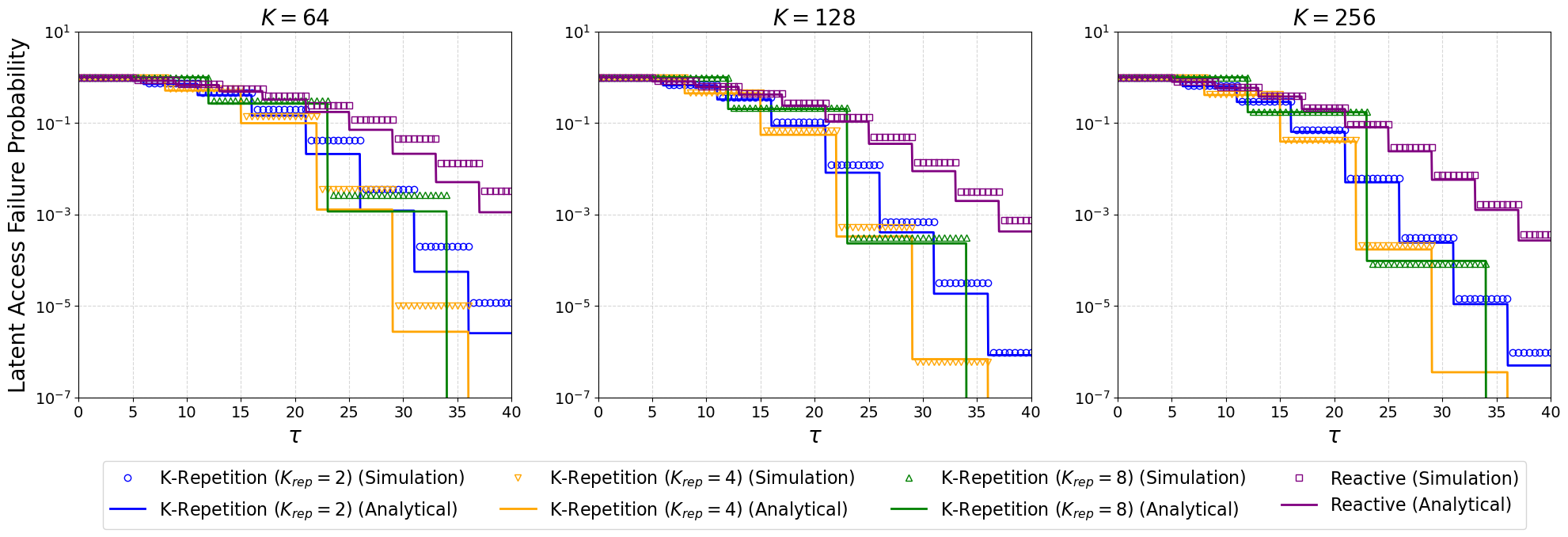
Figure 6: CCDF of the latent access failure probability for $\lambda_{U}=5000$ UE/$\text{km}^{2}$ for the reactive and $K$-repetition HARQ protocols with $K_{rep}=2,4,8$. The plots in the figure show the results for $K=64$, $K=128$ and $K=256$ antennas.

Figs. 5 and 6 show the complementary cumulative distribution function (CCDF) of the latent access probability for a user density of $\lambda_{U}=1000$ UE/$\text{km}^{2}$ and $\lambda_{U}=5000$ UE/$\text{km}^{2}$, respectively. The three plots in each figure display the performance for $64$, $128$ and $256$ antennas, from left to right. The behavior of the performance curves, where the latent access failure probability remains constant for a period of time and then drops on the following TTI, is due to the transmission propagation time on the uplink and the feedback, and the processing times. Fig. 5 depicts the performance with a moderate UE density scenario and shows that the reactive HARQ protocol is the best option for strict delay constraints, with $\tau\leq 6$ TTIs ($0.725$ ms), as there is no time for any of the $K$-repetition configurations to finish their first round-trip. When the first and second round-trips for $K_{rep}=2$ are completed, it has the best performance in $6\leq\tau\leq 8$ TTIs and $11\leq\tau\leq 12$ TTI intervals. From this point on, the best performance is dominated by $K_{rep}=4$ and $K_{rep}=8$, with the best configuration being the one that has more completed round-trips in under $\tau$ TTIs. A similar trend occurs with a higher user density as shown in Fig. 6.

Tables I and II show the reduction in the latent access failure probability upon increasing the number of antennas from $64$ to $256$. There is little improvement for a delay constraint of $1$ ms in either scenario. In applications with a moderate UE density and a delay constraint of $2$ ms or more, we notice an average improvement of around $2$ across both HARQ protocols investigated, while in applications with a higher user density, the failure probability is reduced by as much as $32$ times for $K_{rep}=8$ repetitions and a delay constraint greater or equal to $3$ ms.

HARQ	$T\leq 1$ ms	$T\leq 2$ ms	$T\leq 3$ ms
$K_{rep}=2$	1.25	1.59	1.982
$K_{rep}=4$	1	2.18	1.98
$K_{rep}=8$	1	2.49	-
Reactive	1.12	1.42	1.64

TABLE I: Latent access failure probability reduction in increasing from $64$ to $256$ antennas when $\lambda_{U}=1000$ UE/$\text{km}^{2}$

HARQ	$T\leq 2$ ms	$T\leq 3$ ms	$T\leq 4$ ms
$K_{rep}=2$	1.54	6.81	13.69
$K_{rep}=4$	3.25	17.13	-
$K_{rep}=8$	1.75	32.51	32.51
Reactive	1.40	2.60	6.18

TABLE II: Latent access failure probability reduction in increasing from $64$ to $256$ antennas when $\lambda_{U}=5000$ UE/$\text{km}^{2}$

Nonetheless, notice from Figs. 5 and 6 that increasing the number of antennas from $128$ to $256$ does not change the latency performance significantly. Additionally, the increase in the number of antennas has a larger impact on performance for the higher user density scenario shown in Fig. 6 than for the moderate density one in Fig. 5. Later in this section, we discuss why this happens and how to possibly address it.

As the approximation used to derive the results in Section III relies on $K\gg 1$, there is a gap between the analytical and simulation results when $K=64$ as, in this regime, the value of $F_{K}(x)$, and consequently the interference, outside the main lobe are no longer negligible in comparison to the gain on the main lobe.

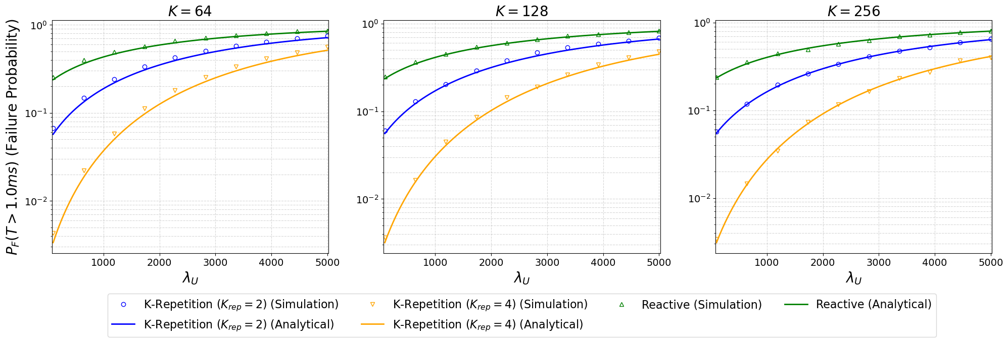
Figure 7: The probability that an UE fails to transmit its packet under $\tau=1$ ms for an user density ranging from $100$ UE/$\text{km}^{2}$. The plots show the results for $K=64$, $K=128$ and $K=256$ antennas, respectively.

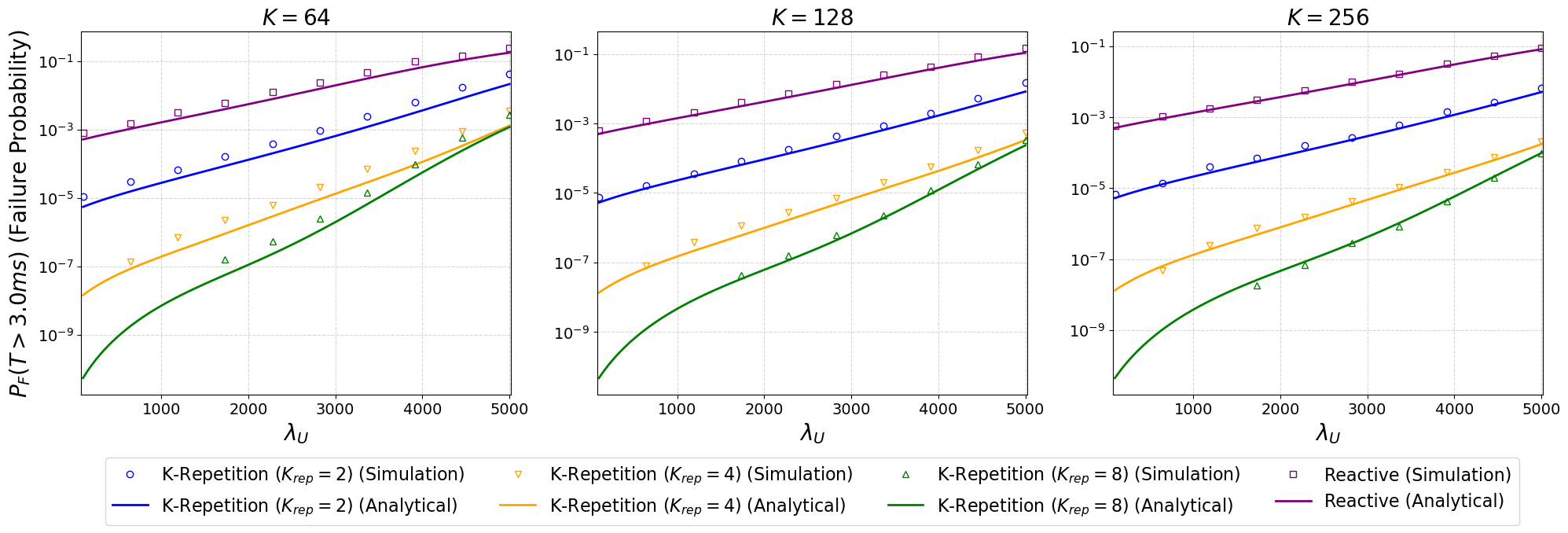
Figure 8: The probability that an UE fails to transmit its packet under $\tau=3$ ms for an user density ranging from $100$ UE/$\text{km}^{2}$. The plots show the results for $K=64$, $K=128$ and $K=256$ antennas, respectively.

Figs. 7 and 8 show how system reliability, i.e., in the probability of transmission failure under the latency constraint $\tau$, scales with an increase in user density for a latency constraint of $\tau=1$ ms and $\tau=3$ ms, respectively. In both figures the user density ranges from $100$ to $5000$ UE/$\text{km}^{2}$. Fig. 7 shows that that the combination of mmWave and massive MIMO is not enough to satisfy the QoS requirement of URLLC applications with the stricter delay constraint (failure probability below $10^{-6}$). Also, in this latency range, the benefit from increasing the number of BS antennas is rather small. For applications with less stringent delay constraints, shown in Fig. 8, the $K$-repetition HARQ protocol with $K_{rep}=4$ and $K_{rep}=8$ is able to support the URLLC QoS requirements. Table III depicts the highest UE density that can be supported by each HARQ and MIMO configuration. When $K_{rep}=4$, increasing the number of BS antennas from $64$ to $128$ increases the supported user density by $11\%$ and increasing the number from $128$ to $256$ increases it by only $7.5\%$. For $K_{rep}=8$, those values are $14\%$ and $5\%$, respectively. It is worth noting that as long as the QoS constraints are satisfied, it is desirable to use the HARQ configuration with the least number of repetitions as possible in order to save UE power.

HARQ	$K=64$ antennas	$K=128$ antennas	$K=256$ antennas
$K_{rep}=2$	-	-	-
$K_{rep}=4$	1800 UE/$\text{km}^{2}$	2000 UE/$\text{km}^{2}$	2150 UE/$\text{km}^{2}$
$K_{rep}=8$	2800 UE/$\text{km}^{2}$	3200 UE/$\text{km}^{2}$	3350 UE/$\text{km}^{2}$
Reactive	-	-	-

TABLE III: User density supported (failure probability below $10^{-6}$) by each configuration.

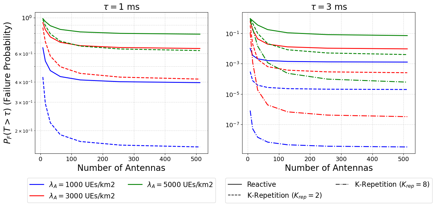
Figure 9: The impact of the number of antennas on the latent access failure probability. The leftmost plot shows results for delay constraint $\tau=1$ ms, while the rightmost for $\tau=3$ ms.

In Fig. 9, we show the impact of increasing the number of antennas on the failure probability for a delay constraint of $\tau=1$ ms on the left and $\tau=3$ ms on the right. From this figure, we can conclude that increasing the number of antennas beyond $100$ for the configuration under consideration ($R=0.5$ km and $\beta=1$) has a decreasing impact on latency performance. Moreover, the $K$-repetition HARQ protocol benefits more from an increased number of antennas than the reactive HARQ protocol does. Also, the plot on the right shows that the latency performance of applications with a moderate latency constraint ($\tau=3$ ms) and higher user densities ($\lambda_{U}\geq 3000$ UE/$\text{km}^{2}$) is greatly improved by changing from traditional MIMO to massive MIMO. This is explained by the capability of producing narrower receiver beams on systems with a higher number of antennas. Nevertheless, as of a certain point, the probability of having a LOS link becomes the dominant bottleneck in reducing the latent access failure probability. As the LOS link probability is unaffected by the number of antennas, another measure must be taken to further reduce the latency. In the system model formulated in this paper, one way to achieve this would be to increase the BS deployment density, effectively decreasing the radius of the cells.

V Conclusions

In this work, we formulated a model to analyze the latency and reliability of mmWave massive MIMO URLLC applications using reactive and $K$-repetition HARQ protocols. We used stochastic geometric spatiotemporal tools to derive closed-form approximations of the system’s latent access failure probability. We validated the analytical results using Monte-Carlo simulations, identifying the limitations of our analytical results. Also, we investigated how the system’s performance is impacted by the application’s latency constraint, the density of UEs served by the system, and the number of antennas in the BS. We concluded that:

• Other than for extremely strict delay constraints ($\tau=0.625$ ms), the $K$-repetition HARQ protocol is a better choice.

• Increasing the number of BS antennas from $64$ to $256$ BS antennas can reduce the latent access failure probability by a factor of 32 for the cell configuration analyzed in the manuscript.

• Massive MIMO’s interference reduction capability significantly improves the reliability of systems with high user density and moderately improves the performance of systems with low user density.

• The increase in reliability from increasing the number of BS antennas beyond $100$ is greatly reduced in the configuration investigated in Section IV, as the probability of having a LOS link between the UE and the BS becomes the main bottleneck.

• Under the configurations investigated in this manuscript, the system can support a UE density as high as $3350$ UE/$\text{km}^{2}$ for a URLLC application with latency and reliability constraints of $3$ ms and $10^{-6}$, respectively.

Overall, we can conclude that it is possible to increase the reliability of URLLC applications by using mmWave massive MIMO, and when this technique is combined with selecting reasonable configuration parameters, these two techniques together can improve reliability under a strict latency constraint ($\tau=1$ ms) and can satisfy URLLC QoS requirements under a less strict latency constraint ($\tau=3$ ms).

Appendix A Proof of Lemma 1

The probability of success in (1) can be expanded to

$$\mathbb{P}\left(\mathrm{SINR}_{m}\geq\gamma\left\lvert TX_{0},N_{m}=n\right.\right)$$ (30)

$$= \mathbb{P}\left\{\left.\left\lvert g_{0}\right\rvert^{2}\geq\frac{\gamma}{\rho K}\left[\sigma^{2}+I\right]\right\rvert TX_{0},N_{m}=n\right\}$$

$$= \exp\left(-\frac{\gamma\sigma^{2}}{\rho K}\right)\mathcal{L}_{I}\left(s\lvert TX_{0},N_{m}=n\right),$$

where $s=\frac{\gamma}{\rho K}$, $I=\underset{x_{i}\in\Phi_{I}}{\sum}\rho\left\lvert g_{i}\right\rvert^{2}F_{K}\left(\frac{\pi}{2}\left(\theta_{0}-\theta_{i}\right)\right)$ is the interference on the typical user’s transmission and $\mathcal{L}_{I}\left(s\lvert\bar{C},x_{0}\in LOS_{m},N_{m}=n\right)$ is the Laplace transform of the interference conditioned on the user not experiencing preamble collision, them having a LOS path, and there being $n$ interferers in the cell.

The Laplace transform of the interference can be derived as (31), shown at the top of the next page.

$$\mathcal{L}_{I}\left(s\lvert TX_{0},N_{m}=n\right) = E_{g_{i},\theta_{i}}\left\{\exp\left[-s\underset{x_{i}\in\Phi_{I}}{\sum}\rho\left\lvert g_{i}\right\rvert^{2}F_{K}\left(\frac{\pi}{2}\left(\theta_{0}-\theta_{i}\right)\right)\right]\right\}$$ (31)

$$= \underset{x_{i}\in\Phi_{I}}{\prod}E_{g_{i},\theta_{i}}\left\{\exp\left[-s\rho\left\lvert g_{i}\right\rvert^{2}F_{K}\left(\frac{\pi}{2}\left(\theta_{0}-\theta_{i}\right)\right)\right]\right\}$$

$$= \underset{x_{i}\in\Phi_{I}}{\prod}E_{\theta_{i}}\left[\frac{1}{1+s\rho F_{K}\left(\frac{\pi}{2}\left(\theta_{0}-\theta_{i}\right)\right)}\right].$$

Unfortunately, obtaining a closed-form expression for the expectation in (31) is not mathematically tractable. Therefore, we first obtain a suitable approximation to the Fejer kernel. Due to the Fejer kernel property in (10), as the number of antennas increases most of the energy is concentrated on the main lobe as shown in Fig. 2. Hence, we choose to approximate it as

$$F_{K}\left(x\right)\approx f_{K}(x)=\begin{cases}-\frac{K^{3}x^{2}}{4}+K\text{, if }x\in\left\{-\frac{2}{K},\frac{2}{K}\right\}\\ 0\text{, otherwise}.\end{cases}$$ (32)

The quadratic approximation in (32) renders the derivation of the expectation in (31) tractable. Furthermore, it ensures that $f_{K}(x)=0$ whenever $x\notin\left(-\frac{2}{K},\frac{2}{K}\right)$, i.e., the contributions of the signals arriving from directions outside of the main lobe to the interference is zero, and that $F_{K}\left(0\right)=f_{K}(0)=K$. Hence,

$$\underset{x_{i}\in\Phi_{I}\cap\theta_{i}\in\left(-\frac{2}{K},\frac{2}{K}\right)}{\prod}E_{\theta_{i}}\left[\frac{1}{1+s\rho F_{K}\left(\frac{\pi}{2}\left(\theta_{0}-\theta_{i}\right)\right)}\right]$$

$$\overset{(a)}{=}\underset{x_{i}\in\Phi_{I}\cap\theta_{i}\in\left(-\frac{2}{K},\frac{2}{K}\right)}{\prod}\frac{\tanh^{-1}\left(\sqrt{\frac{\gamma}{1+\gamma}}\right)}{\sqrt{\gamma\left(1+\gamma\right)}}$$

$$\overset{(b)}{=}\underset{n^{\prime}=0}{\overset{n}{\sum}}{n\choose n^{\prime}}\left(\frac{2}{K}\right)^{n^{\prime}}\left(1-\frac{2}{K}\right)^{n-n^{\prime}}$$

$$\times\left[\frac{\tanh^{-1}\left(\sqrt{\frac{\gamma}{1+\gamma}}\right)}{\sqrt{\gamma\left(1+\gamma\right)}}\right]^{n^{\prime}}$$ (33)

where $(a)$ is obtained from $\int\frac{1}{1-x^{2}}dx=\tanh^{-1}(x)$. While step $(b)$ comes from the fact that the interferers’ angles are uniformly distributed, given that there are $n$ interferers in the cell, the number of interferers within the typical user’s main lobe direction follows a binomial distribution with $n^{\prime}\sim Binomial\left(\frac{2}{K}\right)$. Thus, the conditional success probability can be obtained by summing the marginal distribution weighted by $n^{\prime}$’s probability mass function (PMF). This completes the proof.

Appendix B Proof of Lemma 2

In order for a $K$-repetition HARQ transmission attempt to be successful at least one of the repetitions must be successfully decoded. Therefore, the probability that the $m$-th retransmission attempt is successful, conditioned on no preamble collisions, a LOS path and $n$ interferers, can be obtained as the complement probability that all repetitions fail , as derived in (34), shown at the top of the next page,

$$\mathbb{P}\left(\underset{l=1}{\overset{K_{rep}}{\bigcup}}\mathrm{SINR}_{m,l}\geq\gamma\left\lvert TX_{0},N_{m}=n\right.\right) = 1-\mathbb{P}\left(\underset{l=1}{\overset{K_{rep}}{\bigcap}}\mathrm{SINR}_{m,l}<\gamma\left\lvert TX_{0},N_{m}=n\right.\right)$$ (34)

$$\overset{(a)}{=} 1-\underset{l=1}{\overset{K_{rep}}{\prod}}\left[1-\mathbb{P}\left(\mathrm{SINR}_{m,l}\geq\gamma\left\lvert TX_{0},N_{m}=n\right.\right)\right]$$

$$\overset{(b)}{=} 1-\left[1-\mathbb{P}\left(\mathrm{SINR}_{m}\geq\gamma\left\lvert TX_{0},N_{m}=n\right.\right)\right]^{K_{rep}}$$

$$\overset{(c)}{=} \underset{l=1}{\overset{K_{rep}}{\sum}}{K_{rep}\choose l}\left(-1\right)^{l+1}$$

$$\mathbb{P}\left(\mathrm{SINR}_{m}\geq\gamma\left\lvert TX_{0},N_{m}=n\right.\right)^{l}$$

where step $(a)$ follows from the fact that the set of interferers is different from one repetition to the next, as a new subcarrier is randomly selected for every repetition by each UE, making the SINRs on distinct repetitions mutually independent. Also, as the SINR of every repetition is affected by an interferer process having the same intensity, the probability of success of each repetition is equal, which justifies step $(b)$. Finally, step $(c)$ is obtained from the binomial expansion of the power term. If we work from (34) and follow the same steps derived in Appendix A, we obtain (2), which completes the proof.

References

- [1] ITU, “IMT vision–framework and overall objectives of the future development of IMT for 2020 and beyond,” International Telecommunication Union, Recommendation ITU, 2015.
- [2] E. Bjornson, E. Larsson, and A. Lozano, “16. 6G and the Physical Layer (with Angel Lozano),” Dec 2021. [Online]. Available: https://open.spotify.com/show/0RDeni3rDUx5HnZWJGACqO
- [3] 3GPP, “Study on scenarios and requirements for next generation access technologies,” 3rd Generation Partnership Project (3GPP), Technical Report (TR) 36.913, Jul 2020, version 16.0.0.
- [4] M. Vilgelm, S. Schiessl, H. Al-Zubaidy, W. Kellerer, and J. Gross, “On the reliability of LTE random access: Performance bounds for machine-to-machine burst resolution time,” in IEEE International Conference on Communications (ICC), May 2018, pp. 1–7.
- [5] 3GPP, “Study on New Radio (NR) access technology,” 3rd Generation Partnership Project (3GPP), Technical Report (TR) 38.912, Sept 2018, version 15.0.0.
- [6] A. A. Zaidi, R. Baldemair, V. Moles-Cases, N. He, K. Werner, and A. Cedergren, “OFDM numerology design for 5G new radio to support IoT, eMBB, and MBSFN,” IEEE Commun. Standards Mag., vol. 2, no. 2, pp. 78–83, June 2018.
- [7] 3GPP, “Physical layer procedures for control,” 3rd Generation Partnership Project (3GPP), Technical Specification (TS) 38.213, Apr 2018, version 16.5.0.
- [8] G. Karadag, R. Gul, Y. Sadi, and S. Coleri Ergen, “QoS-constrained semi-persistent scheduling of machine-type communications in cellular networks,” IEEE Trans. Wireless Commun., vol. 18, no. 5, pp. 2737–2750, Apr 2019.
- [9] 3GPP, “Grant-free transmission for UL URLLC,” 3rd Generation Partnership Project (3GPP), TSG RAN WG1 Meeting 88b 38.213, Apr 2017.
- [10] J. Kim, G. Lee, S. Kim, T. Taleb, S. Choi, and S. Bahk, “Two-step random access for 5G system: Latest trends and challenges,” IEEE Netw., vol. 35, no. 1, pp. 273–279, Feb 2021.
- [11] L. Lu, G. Y. Li, A. L. Swindlehurst, A. Ashikhmin, and R. Zhang, “An overview of massive MIMO: Benefits and challenges,” IEEE J. Sel. Topics Signal Process., vol. 8, no. 5, pp. 742–758, Mar 2014.
- [12] E. G. Larsson, O. Edfors, F. Tufvesson, and T. L. Marzetta, “Massive MIMO for next generation wireless systems,” IEEE Commun. Mag., vol. 52, no. 2, pp. 186–195, Feb 2014.
- [13] E. Björnson, J. Hoydis, and L. Sanguinetti, “Massive MIMO has unlimited capacity,” IEEE Trans. Wireless Commun., vol. 17, no. 1, pp. 574–590, Nov 2018.
- [14] T. L. Marzetta, E. G. Larsson, H. Yang, and H. Q. Ngo, Fundamentals of Massive MIMO. Cambridge University Press, 2016.
- [15] T. S. Rappaport, S. Sun, R. Mayzus, H. Zhao, Y. Azar, K. Wang, G. N. Wong, J. K. Schulz, M. Samimi, and F. Gutierrez, “Millimeter wave mobile communications for 5g cellular: It will work!” IEEE Access, vol. 1, pp. 335–349, May 2013.
- [16] S. Rangan, T. S. Rappaport, and E. Erkip, “Millimeter-wave cellular wireless networks: Potentials and challenges,” Proc. IEEE, vol. 102, no. 3, pp. 366–385, Nov 2014.
- [17] J. G. Andrews, T. Bai, M. N. Kulkarni, A. Alkhateeb, A. K. Gupta, and R. W. Heath, “Modeling and analyzing millimeter wave cellular systems,” IEEE Trans. Commun., vol. 65, no. 1, pp. 403–430, Oct 2017.
- [18] Z. Sattar, J. V. C. Evangelista, G. Kaddoum, and N. Batani, “Analysis of the cell association for decoupled wireless access in a two tier network,” in IEEE 28th Annual International Symposium on Personal, Indoor, and Mobile Radio Communications (PIMRC), Feb 2017, pp. 1–6.
- [19] ——, “Antenna array gain and capacity improvements of ultra-wideband millimeter wave systems using a novel analog architecture design,” IEEE Wireless Commun. Lett., vol. 9, no. 3, pp. 289–293, Nov 2019.
- [20] ——, “Spectral efficiency analysis of the decoupled access for downlink and uplink in two-tier network,” IEEE Trans. Veh. Technol., vol. 68, no. 5, pp. 4871–4883, Feb 2019.
- [21] Y. Gao and L. Dai, “Random access: Packet-based or connection-based?” IEEE Trans. Wireless Commun., vol. 18, no. 5, pp. 2664–2678, May 2019.
- [22] Y. Liu, Y. Deng, H. Zhou, M. Elkashlan, and A. Nallanathan, “A general deep reinforcement learning framework for grant-free NOMA optimization in mURLLC,” arXiv preprint arXiv:2101.00515, Mar 2021.
- [23] J. V. C. Evangelista, Z. Sattar, G. Kaddoum, B. Selim, and A. Sarraf, “Intelligent link adaptation for grant-free access cellular networks: A distributed deep reinforcement learning approach,” Jul 2021.
- [24] K. Lai, J. Lei, Y. Deng, L. Wen, and G. Chen, “Analyzing uplink grant-free sparse code multiple access system in massive IoT networks,” arXiv preprint arXiv:2103.10241, Mar 2021.
- [25] J. V. Evangelista, Z. Sattar, and G. Kaddoum, “Analysis of contention-based scma in mmtc networks,” in IEEE Latin-American Conference on Communications (LATINCOM), Nov 2019, pp. 1–6.
- [26] J. Ding, D. Qu, H. Jiang, and T. Jiang, “Success probability of grant-free random access with massive MIMO,” IEEE Internet Things J., vol. 6, no. 1, pp. 506–516, Sept 2019.
- [27] M. Gharbieh, H. ElSawy, H.-C. Yang, A. Bader, and M.-S. Alouini, “Spatiotemporal model for uplink IoT traffic: Scheduling and random access paradox,” IEEE Trans. Wireless Commun., vol. 17, no. 12, pp. 8357–8372, Oct 2018.
- [28] N. Jiang, Y. Deng, X. Kang, and A. Nallanathan, “Random access analysis for massive IoT networks under a new spatio-temporal model: A stochastic geometry approach,” IEEE Trans. Commun., vol. 66, no. 11, pp. 5788–5803, Jul 2018.
- [29] T. Jacobsen, R. Abreu, G. Berardinelli, K. Pedersen, P. Mogensen, I. Z. Kovács, and T. K. Madsen, “System level analysis of uplink grant-free transmission for URLLC,” in IEEE Globecom Workshops (GC Wkshps). IEEE, Jan 2017, pp. 1–6.
- [30] Y. Liu, Y. Deng, M. Elkashlan, A. Nallanathan, and G. K. Karagiannidis, “Analyzing grant-free access for URLLC service,” IEEE J. Sel. Areas Commun., vol. 39, no. 3, pp. 741–755, Aug 2020.
- [31] X. Lu, M. Salehi, M. Haenggi, E. Hossain et al., “Stochastic geometry analysis of spatial-temporal performance in wireless networks: A tutorial,” arXiv preprint arXiv:2102.00588, Feb 2021.
- [32] Y. Hmamouche, M. Benjillali, S. Saoudi, H. Yanikomeroglu, and M. D. Renzo, “New trends in stochastic geometry for wireless networks: A tutorial and survey,” Proc. IEEE, vol. 109, no. 7, pp. 1200–1252, Mar 2021.
- [33] N. Jiang, Y. Deng, A. Nallanathan, X. Kang, and T. Q. S. Quek, “Analyzing random access collisions in massive IoT networks,” IEEE Transactions on Wireless Communications, vol. 17, no. 10, pp. 6853–6870, Aug 2018.
- [34] R. Tanbourgi, H. S. Dhillon, and F. K. Jondral, “Analysis of joint transmit–receive diversity in downlink MIMO heterogeneous cellular networks,” IEEE Trans. Wireless Commun., vol. 14, no. 12, pp. 6695–6709, Jul 2015.
- [35] T. M. Nguyen, Y. Jeong, T. Q. Quek, W. P. Tay, and H. Shin, “Interference alignment in a Poisson field of MIMO femtocells,” IEEE Trans. Wireless Commun., vol. 12, no. 6, pp. 2633–2645, Apr 2013.
- [36] A. Adhikary, H. S. Dhillon, and G. Caire, “Massive-MIMO meets HetNet: Interference coordination through spatial blanking,” IEEE J. Sel. Areas Commun., vol. 33, no. 6, pp. 1171–1186, Mar 2015.
- [37] N. Lee, D. Morales-Jimenez, A. Lozano, and R. W. Heath, “Spectral efficiency of dynamic coordinated beamforming: A stochastic geometry approach,” IEEE Trans. Wireless Commun., vol. 14, no. 1, pp. 230–241, Jul 2014.
- [38] L. H. Afify, H. ElSawy, T. Y. Al-Naffouri, and M.-S. Alouini, “A unified stochastic geometry model for MIMO cellular networks with retransmissions,” IEEE Trans. Wireless Commun., vol. 15, no. 12, pp. 8595–8609, Oct 2016.
- [39] Z. Ding, P. Fan, and H. V. Poor, “Random beamforming in millimeter-wave NOMA networks,” IEEE Access, vol. 5, pp. 7667–7681, Feb 2017.
- [40] M. Haenggi, Stochastic geometry for wireless networks. Cambridge University Press, 2012.
- [41] W. Lu and M. Di Renzo, “Stochastic geometry modeling of cellular networks: Analysis, simulation and experimental validation,” in Proceedings of the 18th ACM International Conference on Modeling, Analysis and Simulation of Wireless and Mobile Systems, Nov 2015, pp. 179–188.
- [42] H. ElSawy and E. Hossain, “On stochastic geometry modeling of cellular uplink transmission with truncated channel inversion power control,” IEEE Trans. Wireless Commun., vol. 13, no. 8, pp. 4454–4469, Apr 2014.
- [43] A. Thornburg, T. Bai, and R. W. Heath, “Performance analysis of outdoor mmWave ad hoc networks,” IEEE Trans. Signal Process., vol. 64, no. 15, pp. 4065–4079, Apr 2016.
- [44] G. Lee, Y. Sung, and J. Seo, “Randomly-directional beamforming in millimeter-wave multiuser MISO downlink,” IEEE Trans. Wireless Commun., vol. 15, no. 2, pp. 1086–1100, Sep 2015.
- [45] J. E. Marsden, M. J. Hoffman et al., Elementary classical analysis. Macmillan, 1993.
- [46] F. Baccelli and B. Błaszczyszyn, Stochastic geometry and wireless networks. Now Publishers Inc, 2009, vol. 1.
- [47] 3GPP, “5G NR User Equipment (UE) radio transmission and reception; Part 3: Range 1 and Range 2 Interworking operation with other radios,” 3rd Generation Partnership Project (3GPP), Technical Specification (TS) 38.101, Apr 2021, version 16.7.0.
- [48] ——, “5G NR Physical channels and modulation,” 3rd Generation Partnership Project (3GPP), Technical Specification (TS) 38.211, Apr 2021, version 16.5.0.