[table]capposition=top \newfloatcommandcapbtabboxtable[][\FBwidth]
CCVS: Context-aware Controllable Video Synthesis
Abstract
This presentation introduces a self-supervised learning approach to the synthesis of new video clips from old ones, with several new key elements for improved spatial resolution and realism: It conditions the synthesis process on contextual information for temporal continuity and ancillary information for fine control. The prediction model is doubly autoregressive, in the latent space of an autoencoder for forecasting, and in image space for updating contextual information, which is also used to enforce spatio-temporal consistency through a learnable optical flow module. Adversarial training of the autoencoder in the appearance and temporal domains is used to further improve the realism of its output. A quantizer inserted between the encoder and the transformer in charge of forecasting future frames in latent space (and its inverse inserted between the transformer and the decoder) adds even more flexibility by affording simple mechanisms for handling multimodal ancillary information for controlling the synthesis process (e.g., a few sample frames, an audio track, a trajectory in image space) and taking into account the intrinsically uncertain nature of the future by allowing multiple predictions. Experiments with an implementation of the proposed approach give very good qualitative and quantitative results on multiple tasks and standard benchmarks.
1 Introduction
Feeding machines with extensive video content, and teaching them to create new samples on their own, may deepen their understanding of both the physical and social worlds. Video synthesis has numerous applications from content creation (e.g., deblurring, slow motion) to human-robot interaction (e.g., motion prediction). Despite the photo-realistic results of modern image synthesis models [38], video synthesis is still lagging behind due to the increased complexity of the additional temporal dimension.
An emerging trend is to use autoregressive models, for example transformer architectures [68], for their simplicity, and their ability to model long-range dependencies and learn from large volumes of data [16, 4]. First introduced for natural language processing (NLP) and then succesfully applied to visual data [18], the strength of transformers is grounded in a self-attention mechanism which considers all pairwise interactions within the data. The price to pay is a computational complexity which grows quadratically with the data size, which itself depends linearly on the temporal dimension and quadratically on the spatial resolution in the image domain. Although there have been some efforts to reduce the complexity of self-attention [50, 39, 11], using such methods directly on visual data is still limited to low resolutions and impractical without considerable computational power [9, 79].
Some recent works [20, 53] address this problem by using an autoencoder to compress the visual data, and apply the autoregressive model in the latent space. This greatly reduces the memory footprint and computational cost, yet, the greater the compression, the harder it is to faithfully reconstruct frames. The corresponding trade-offs may undermine the practical usability of these approaches. GANs [26] mitigate this issue by “hallucinating” plausible local details in image synthesis [20]. But latent video transformers [53] decode frames independently, which prevents local details from being temporally coherent. Hence, using GANs in this setting may result in flickering effects in the synthesized videos.
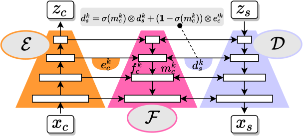
We follow the problem decomposition from [53, 20], but introduce a more elaborate compression strategy with CCVS (for Context-aware Controllable Video Synthesis), an approach that takes advantage of “context” frames (i.e., both input images and previously synthesized ones) to faithfully reconstruct new ones despite lossy compression. As shown in Figure 1, CCVS relies on optical flow estimation between context and new frames, within temporal skip connections, to let information be shared across timesteps. New content, which cannot be retrieved from context, is synthesized directly from latent compressed features, and adversarial training [26] is used to make up realistic details. Indeed, information propagates in CCVS to new frames as previously synthesized ones become part of the context. Like other video synthesis architectures based on autoregressive models [79, 53], CCVS can be used in many tasks besides future video prediction. Any data which can be expressed in the form of a fixed-size sequence of elements from a finite set (aka, tokens) can be processed by a transformer. This applies to video frames (here, via compression and quantization) and to other types of data. Hence, one can easily fuse modalities without having to build complex or task-specific architectures. This idea has been used to control image synthesis [20, 54], and we extend it to a variety of video synthesis tasks by guiding the prediction with different annotations as illustrated in Figure 2. Code, pretrained models, and video samples synthesized by our approach are available at the url https://16lemoing.github.io/ccvs. Our main contributions are as follows:
-
1.
an optical flow mechanism within an autoencoder to better reconstruct frames from context,
-
2.
the use of ancillary information to control latent temporal dynamics when synthesizing videos,
-
3.
a performance on par with or better than the state of the art, while being more memory-efficient.
2 Related Work
Video synthesis.
In its simplest form, videos are produced without prior information about their content. GAN-based approaches map Gaussian noise into a visually plausible succession of frames. For example, VGAN [71] and ProgressiveVGAN [1], adapt the traditional GAN framework [26] from image to video synthesis by simply using 3D instead of 2D convolutions. These approaches, including recent attempts such as G3AN [76], are computationally expensive, and, by nature, restricted to synthesizing a fixed number of frames due to the constraints of their architecture. Other approaches predict latent motion vectors with a CNN [56], or a recurrent neural network (RNN) [65, 12, 57], and generate frames with individual 2D operations. To avoid the shortcomings of information loss in the sequential processing of RNNs, we use an attention-based autoregressive model instead. Since we forecast temporal dynamics in a compressed space, a large temporal window can be used when predicting new frames, without having to resort to expensive 3D computations. Previous works have attempted to scale video synthesis to higher resolution by using progressive training [1], sub-sampling [56, 57], reducing the dimension of the discriminator [36], or redefining the task as finding a trajectory in the latent space of a pre-trained image generator [63]. Compression, together with efficient context-aware reconstruction allows us to synthesize videos at high resolution.
Controllable video synthesis.
Some of the aforementioned works [56, 12, 57, 76] handle synthesis conditioned on a class label. Another popular control is to use a few priming frames to set off the generation process. This task, known as future video prediction, has received a lot of attention recently. Methods based on variational autoencoders (VAE) [2, 15] have been proposed to account for the stochastic nature of future forecasting, i.e., the plurality of possible continuations, disregarded in deterministic predictive models [21, 47, 70]. Yet, their blurry predictions have motivated the incorporation of adversarial training [44], hierarchical architectures [7, 80], fully latent temporal models [22], or normalizing flows [42]. Another line of work infers spatial transformation parameters (e.g., optical flow), and predicts the future by warping past frames (i.e., grid sampling and interpolation as in [33]) in RGB space [21, 72, 28, 24, 81] or in feature space [45], typically using a refinement step to handle occlusions. Lately, autoregressive methods [79, 53] leveraging a self-attention mechanism [68] have also been applied to this task. Our method benefits from the context-efficiency of approaches based on spatial transformation modules and the modeling power of autoregressive networks. In the meantime, other forms of control with interesting applications have emerged. Point-to-point generation [75], a variant of future video prediction, specifies both start and end frames. State or action-conditioned synthesis [28, 48] guides the frame-by-frame evolution with high-level commands. Additional works consider video synthesis based on one [51] or multiple layouts [74, 46], another video [8], or sound [73, 34, 10]. To account for the variety of potential controls, we leverage the flexibility of transformers, and propose an unifying approach to tackle all of these tasks.
3 Context-aware controllable video synthesis
3.1 Overview of the proposed approach
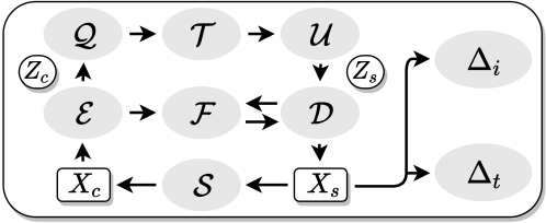
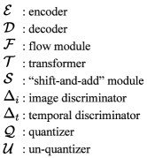
We consider video data, such that an individual frame is natively an element of , which can be encoded as some feature in with reduced spatial resolution and increased number of channels. We assume that we are given in corresponding to successive frames, and our goal is to synthesize a plausible representation of the following frames which lies in . Given , we can compute the corresponding features in using some encoder on each frame individually, then use an autoregressive model (a transformer coupled with a quantization step in our case) to predict features in formed by the features corresponding to time ticks to . (Note that the values of and can be arbitrary, using [by now] traditional masking and sliding window techniques.) These features can finally be converted one by one into the corresponding frames using some decoder .
The overall approach is illustrated by Figure 1. The use of a quantizer over a learned codebook in our implementation complicates the architecture a bit, but has several advantages, including the reuse of familiar NLP technology [68] and, perhaps more importantly, affording simple mechanisms for handling different types of inputs (from images to sound for example [9, 31]) and the intrinsically uncertain and multimodal nature of future prediction (by sampling different codebook elements according to their likelihood [30]). Concretely, this choice simply amounts to inserting in our architecture, right after the encoder , a nearest-neighbor quantizer parameterized by an codebook which, given the embedding of a frame, returns a matrix of corresponding tokens, that is, the indices of the closest entry in the codebook for feature vector for all spatial locations in . We abuse notation, and identify with its parameterization by this codebook, so we can optimize over just as we optimize over instead of naming explicitly its parameters in the rest of this presentation. An “un-quantizer” , also parameterized (implicitly) by the codebook and associating with each token the corresponding entry of the codebook, is also inserted right before the decoder . In this setting, takes as input a sequence of tokens, and outputs the tokens for subsequent frames, each one of them chosen among possibilities as either the one with the highest score, or drawn randomly from the top- scores to account for the multimodal nature of future forecasting (here is some predefined constant, see [30] for related approaches).
The elements of the architecture described so far are by now (individually) rather classical, with learnable, parametric functions , , and . Besides putting them all together, and as detailed in the rest of this section, we add several original elements: (a) The encoding/decoding scheme is improved by the use of two discriminators, and respectively, trained in an adversarial manner to ensure that the predicted frames are realistic and temporally consistent. (b) The context frames are themselves updated each time a new frame is predicted in an autoregressive manner (iteratively fill the sequence up to some predefined capacity, then shift to the left, forgetting the first frame and adding the latest synthetic one on the right). (c) The encoder and decoder are linked through a learnable flow module , allowing the context frames to guide the prediction of the synthetic ones. (d) Additional control variables, ranging from object trajectories to audio tracks, can be used in the form of sequence- or frame-level annotations to drive the synthesis by adding the corresponding tokens to the ones passed on to the autoregressive model .
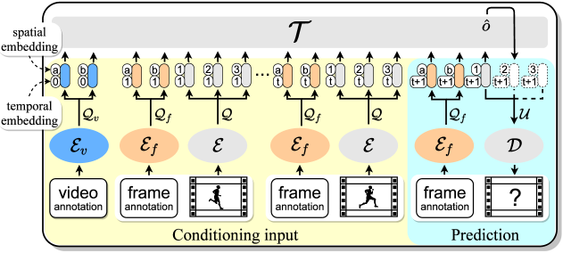
We detail in this section the concrete components of the approach sketched above, including the autoencoder and quantizer architectures and their training procedure (Section 3.2), and the implementation of the autoregressive model by a transformer [68], illustrated in Figure 2, which we adapt to account for outside control signals (Section 3.3), once again with the corresponding procedure. Further architectural choices are also detailed in Appendix A.
3.2 First stage: training the context-aware autoencoder and the quantizer
Architecture.
and respectively decreases and increases the spatial resolution by using convolutional residual blocks [29], with the corresponding resolution levels (). It is common practice to augment, as in U-Net [55], the autoencoder with long skip connections between and to share information across the two models at these intermediate levels and escape the lossy compression bottleneck. Although we cannot apply this directly to our setting since information only flows through for predicted timesteps, such skip connections can be established from the encoding stage of a context frame to the decoding stage of a new frame (resulting from features ). Similar mechanisms [19, 15] have been proposed in the past for video synthesis but they are only copying static background features from a single context frame. We follow works on semantic segmentation [23] and face frontalization [78] and use a flow module to warp features and produce temporally consistent outputs despite motion. We extend this to multi-frame contexts, with significant performance gains and no additional parameter to be learned.
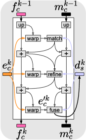
Concretely, let be features being encoded from , and features being decoded from at a given intermediate resolution . We first compute all intermediate context features by applying to . We then progressively decode features for the new frame from low () to high resolution () by iterating over the following steps: (a) apply one decoding sub-module to get from , (b) use to refine the optical flow (in ) which estimates the displacement field from to (as a proxy to the one from to ), and a fusion mask (in ) which indicates the expected similarity between aligned features and (also as a proxy for the one in image domain) with corresponding to a standard warping operation, (c) use and to update with context information (see update rule (1) below), (d) move to resolution level by going back to (a). We note that estimates and in a coarse-to-fine fashion by refining and (see Appendix A for further details). Temporal skip connections at a given resolution level are defined as the following in-place modification of :
| (1) |
where is the Sigmoid function, and the element-wise product. We note that update rule (1) is quite standard for warping and fusing two streams of spatial information [74, 28, 23]. For concrete implementation of , we build upon LiteFlowNet [32], an optical flow estimation model which also combines pyramidal extraction and progressive warping of features. For simple integration into our framework, we use features from and both in the mask and flow estimation, and in the update (1). This process readily generalizes to multi-frame contextual information (see Appendix D for details). Similar to spatial transformers [33], the warping operation is differentiable. As a result, gradients from the training losses can backpropagate from to through . This allows end-to-end training of the autoencoder even with information from different timesteps in and .
Training procedure.
The global objective is the linear combination of four auxiliary ones:
| (2) |
namely a quantization loss (), a reconstruction loss (), an adversarial loss (), and a contextual loss (), detailed in the next paragraphs.
The codebook is trained by minimizing the reconstruction error between encoded features and quantized features (with notations introduced in Section 1):
| (3) |
where is the stop gradient operation which constrains its operand to remain constant during backpropagation. The first part moves the codebook entries closer to the encoded features. The second part, known as the commitment loss [67], reverses the roles played by the two variables.
In regions with complex textures and high frequency details, local patterns shifted by a few pixels in and its reconstruction may result in large pixel-to-pixel errors, while being visually satisfactory. We thus define the recovery objective as the loss in both RGB space and between features from a network [59] pretrained on ImageNet [14]:
| (4) |
To tackle cases where information cannot be recovered from context due to occlusion, and the compressed features are insufficient to create plausible reconstructions due to lossy compression, we supplement our architecture with an image discriminator , made of downsampling residual blocks [29], to encourage realistic outputs. tries to distinguish real images from reconstructed ones (), while and fools into assuming reconstructed images are as good as real ones ():
We employ a similar strategy on sequences of consecutive frames to improve the temporal consistency using a 3D temporal discriminator , a direct extension of 2D image discriminator .
The success of our method relies on accurate motion estimation in , a difficult task which benefits from self-supervision [35]. Therefore, we train the autoencoder with augmented views of the input frames as context. Custom augmentations functions include: rotation, scaling, translation, elastic deformation, and combinations of these. Augmented views are obtained by warping by the suitable flow : , and the inverted flow from to can be approximated.111Our implementation of flow inversion approximation is detailed in Appendix C. We resort to flow inversion because directly reconstructing distorted views may encourage similar defects during inference. Moreover, we balance between self-recovery and context-recovery objectives by additionally applying a blurring function and an occlusion mask to the augmented frames . This augmentation strategy is illustrated in Appendix F. We define the contextual loss as:
| (7) |
where , and and are the flow and mask estimated by . In practice, this loss is applied at intermediate resolution levels for improved training.
3.3 Second stage: predicting temporal dynamics with transformers

Architecture.
We follow [20] and adopt an architecture similar to Image-GPT [9] for . Instead of modeling a single annotated frame as in [54], we design our model to account for sequences of such frames to allow prediction of temporal dynamics controlled by ancillary information in the form of video- and frame-level annotations. We have shown, in Section 3.2, how to represent a frame as a sequence of tokens (indices in ) through encoding and quantization. Similar strategies can be applied to cater to other types of data, with or without compression depending on their complexity, and, thereby, turn ancillary information into tokens as well. The capacity of the transformer (the maximum sequence length it can process) is , where and are the size of video- and frame-level annotations respectively. The final layer of the model predicts, for every in , a vector (of size , the number of possible tokens) which scores the likelihood of the th token given all preceding ones.
Training procedure.
To learn the parameters of , we load a complete sequence ( frames corresponding to tokens), and try to predict the last tokens based on the first ones. This is done by maximizing the log-likelihood of the data using the cross-entropy loss:
| (8) |
where is the th ground-truth token, and a vector of 0’s with a in its th coordinate.
Inference.
During inference we use to complete autoregressively an input sequence of tokens. To avoid known pitfalls (e.g., repetitive synthesis) and allow diverse outcomes, we use top- sampling whereby the next token is randomly chosen among the most likely ones, weighted by their scores . Although processes sequences of annotated frames, we predict ones of arbitrary length by using a temporal sliding window. Tokens corresponding to video- and frame-level annotations are given as input to (not predicted, even for future frames) to guide the synthesis. We show in the experiments how this control can translates into a variety of interesting tasks.
4 Experiments
We assess the merits of CCVS in the light of extensive experiments on various video synthesis tasks.
Datasets.
BAIR Robot Pushing [19] consists of 43k training and 256 test videos of a robotic arm interacting with objects from a fixed viewpoint. A high-resolution version has recently been released. We manually annotate, in frames, the location of the arm in image space to train a position estimator, which we use for state-conditioned synthesis. To account for real world scenarios, we evaluate on Kinetics-600 [5], a large and diverse action-recognition dataset with approximately 500K videos. We also test our method on AudioSet-Drums [25] for sound-conditioned synthesis on music performance, containing 6k and 1k video clips in train and test splits respectively. Other datasets and tasks are covered in Appendix E.
Metrics.
We use the Fréchet video distance (FVD) [66] which measures the distribution gap between real and synthetic videos in the feature space of an Inception3D network [6] pretrained on Kientics-400 [40]. It estimates the visual quality and temporal consistency of samples as well as the diversity in unconditioned scenarios. In conditioned ones, we use another metric for diversity (DIV) which is the mean pixel-wise distance among synthetic trajectories conditioned on the same input. For near-deterministic motions (e.g., in reconstructions, or constrained tasks), there is a one-to-one mapping between real video frames and synthetic ones, and we include pairwise image quality assessments: the structural similarity index measure (SSIM) [77] which evaluates a per-frame conformity (combination of luminance, contrast and structure), and the peak signal-to-noise ratio (PSNR) which is directly related to the root mean squared error. For each metric, we compute the mean and standard deviation (std) over evaluation runs (2 for Kinetics due to its voluminous 50k video test set). For clarity, the std value is shown only when it is greater than the reported precision.
Training details.
All our models are trained on 4 Nvidia V100 GPUs (32GB VRAM each), using ADAM [41] optimizer, for multiple 20 hour runs. We adapt the batch size to fill the memory available. We use a learning rate of to train the autoencoder, and exponential moving average [83] to obtain its final parameters. We use weighting factors and for and in Equations (2) and (3) respectively. We use a learning rate of to train the transformer.
4.1 Ablation study
| Self-recovery | Ctxt.-recovery | Reconstruction | State-conditioned | Pred. | Unc. | |||||||||||
| RGB | VGG | Sup. | Ctxt. | FVD | PSNR | FVD | PSNR | FVD | FVD | |||||||
| ✓ | 0 | |||||||||||||||
| [0pt][0pt] ✓ | ✓ | 0 | ||||||||||||||
| ✓ | ✓ | ✓ | 0 | |||||||||||||
| [0pt][0pt] ✓ | ✓ | ✓ | ✓ | 0 | ||||||||||||
| ✓ | ✓ | ✓ | ✓ | ✓ | 1 | |||||||||||
| [0pt][0pt] ✓ | ✓ | ✓ | ✓ | ✓ | ✓ | 1 | ||||||||||
| ✓ | ✓ | ✓ | ✓ | ✓ | ✓ | 8 | ||||||||||
| [0pt][0pt] ✓ | ✓ | ✓ | ✓ | ✓ | ✓ | 15 | ||||||||||
| Training longer (num. epochs ) | ||||||||||||||||
| “Sup.”: self-supervision of ; “Ctxt.”: number of context frames taken into account (in ) when decoding current frame (in ). | ||||||||||||||||
| Architecture | Top-k | State-conditioned | Pred. | Unc. | ||||
| Layer | Head | Dec. | Frame | State | FVD | PSNR | FVD | FVD |
| 6 | 4 | 1 | 1 | |||||
| [0pt][0pt] 12 | 8 | 1 | 1 | |||||
| 24 | 16 | 1 | 1 | |||||
| [0pt][0pt] 24 | 16 | ✓ | 1 | 1 | ||||
| 24 | 16 | ✓ | 10 | 1 | ||||
| [0pt][0pt] 24 | 16 | ✓ | 100 | 1 | ||||
| 24 | 16 | ✓ | 100 | 10 | ||||
| “Dec.”: spatio-temporal decomposition of positional embeddings. | ||||||||
[\FBwidth]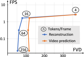
We conduct an ablation study of CCVS to show the individual contribution of the key components of the proposed autoencoder (Table 1), transformer (Table 4), and the effect of compression (Figure 4).
First, we fix the transformer and observe the incremental improvements in synthesis quality when adding self- and context-recovery modules to the autoencoder (Table 1). In particular, loss in the feature space of a net [59] produces sharper videos than using the same loss in the RGB space alone. Predicted frames using image and temporal discriminators ( and ) display greater realism and temporal consistency. The flow module significantly improves the performance on all metrics by allowing context frames to guide the reconstruction of synthetic ones. The self-supervision of , the use of larger context windows, and longer training times, further improve the quality of the synthesis. seems to deteriorate the FVD at first, but when all modules are combined it improves FVD by almost a factor as it encourages better temporal consistency in the presence of context.
We fix the autoencoder, and compare different architectures and sampling strategies for the transformer (Table 4). Increasing the model capacity by adding layers and increasing expressivity (number of attention heads) along with a spatio-temporal decomposition of positional embeddings (shown in Figure 2, detailed in supplementary material) yields small improvements. Top- sampling is beneficial for stochastic tasks (video prediction and unconditional synthesis), whereas always selecting the most probable tokens results in little to no motion. Guiding temporal dynamics with state-conditioned synthesis reduces the advantage of sampling by narrowing down possible outcomes.
Finally, we explore the effect of compression (in terms of the number of tokens for each frame) on synthesis speed (FPS) and quality (FVD) of reconstructed and predicted videos (Figure 4). We use a compression of tokens in our default setup since it gives the best FVD while retaining a reasonable speed. The critical drop of FPS for low compression ratios is due to the pairwise consideration of all input tokens in . Note that using a smaller temporal window in may allow additional speed-ups.
4.2 Quantitative and qualitative studies
| Method | Cond. | FVD | Code Avail. | Memory, compute |
| MoCoGAN [65] | 4 | ✓ | 16GB, 23h∗ | |
| SVG-FP [15] | 2 | ✓ | 12GB, 6 to 24h∗ | |
| CDNA [21] | 2 | ✓ | 10GB, 20h∗ | |
| SV2P [2] | 2 | ✓ | 16GB, 24 to 48h∗ | |
| SRVP [22] | 2 | ✓ | 36GB, 168h∗ | |
| VideoFlow [42] | 3 | 128GB, 336h∗ | ||
| LVT [53] | 1 | ✓ | 128GB, 48h | |
| SAVP [44] | 2 | ✓ | 32GB, 144h | |
| DVD-GAN-FP [12] | 1 | 2TB, 24h∗ | ||
| Video Transformer (S) [79] | 1 | 256GB, 33h∗ | ||
| TriVD-GAN-FP [45] | 1 | 1TB, 280h∗ | ||
| Low res. CCVS (ours) | 1 | ✓ | 128GB, 40h | |
| Video Transformer (L) [79] | 1 | 512GB, 336h∗ | ||
| SSIM () | SSIM () | |||
| High res.∗∗ CCVS (ours) | 1 | 0.729 | 0.683 | |
| + end frame | 2 | 0.766 | 0.839 | |
| + state | 1 | 0.885 | 0.863 | |
| ∗: value confirmed by authors; ∗∗: training / inference / SSIM at , FVD at . | ||||
![[Uncaptioned image]](/html/2107.08037/assets/x6.png)
| Future prediction | 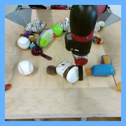 |
 |
 |
 |
 |
 |
 |
 |
 |
|---|---|---|---|---|---|---|---|---|---|
| Point-to- point | 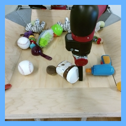 |
 |
 |
 |
 |
 |
 |
 |
 |
| State- conditioned | 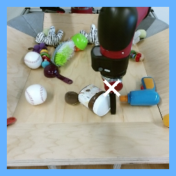 |
 |
 |
 |
 |
 |
 |
 |
 |
| Real video |  |
 |
 |
 |
 |
 |
 |
 |
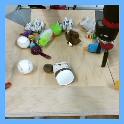 |
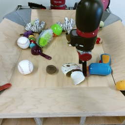
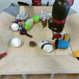
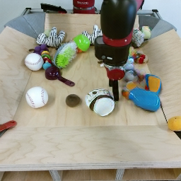
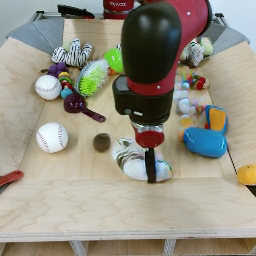
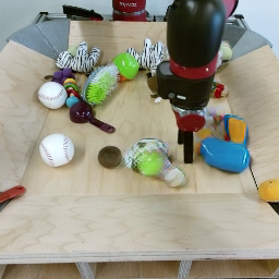
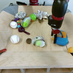
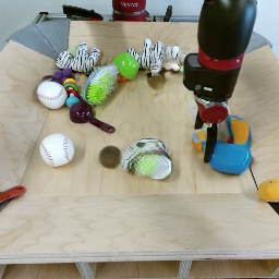
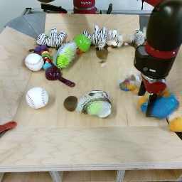
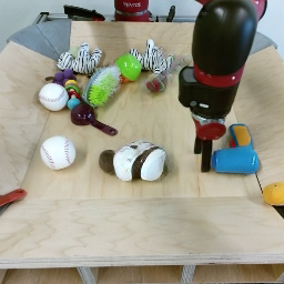
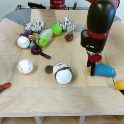
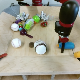
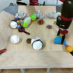
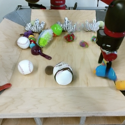
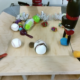
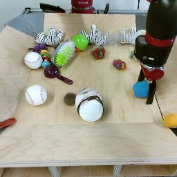
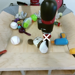
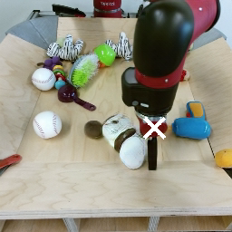
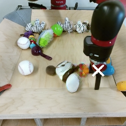
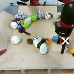
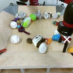
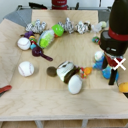
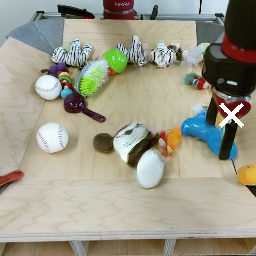
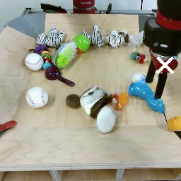
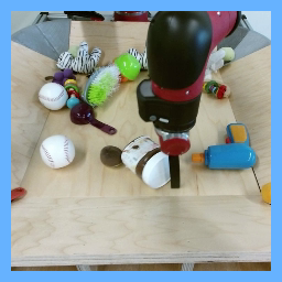
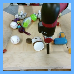
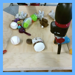
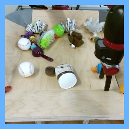
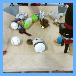
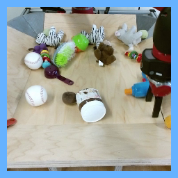
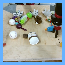
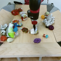
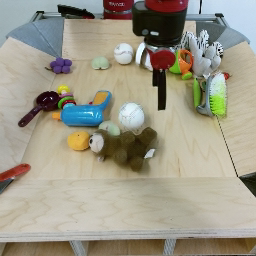
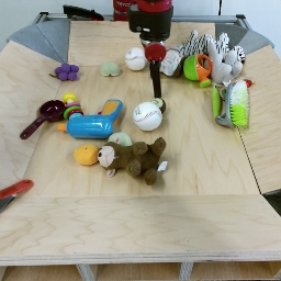
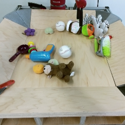
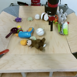
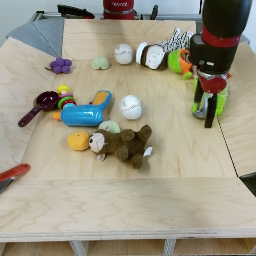
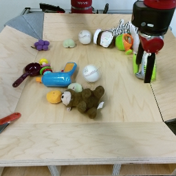
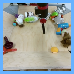
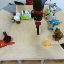
BAIR. For future video prediction on BAIR (Table 2), CCVS trained at resolution (low res.) is on par with the best method (L-size version of [79]), but requires much less computing resources, and outperforms [79] under similar resources. We also propose high res. CCVS which is not strictly comparable to the prior arts as we use image resolution for training and test, and resize the synthesized frames to for computing FVD. However, using this variant demonstrates the performance gains that can arise by scaling CCVS. We additionally address point-to-point synthesis (with the end frame as a video-level annotation) and state-conditioned synthesis (with the estimated 2D position of the arm as a frame-level annotation). Point-to-point synthesis is more difficult than video prediction: Not only does it requires realistic video continuations, but also ones which explain the end position of all visible objects. Hence, FVD score is constant despite the additional input. Still, this yields better SSIM for mid-point and one-before-last frames. State-conditioned synthesis improves on FVD and mid-synthesis SSIM as motion becomes near-deterministic. Some synthetic frames for these tasks are shown in Figure 5. CCVS creates plausible high-quality videos in various settings, and true interactions with objects compared to previous attempts [48] at the same resolution.
| Size | Reconstruction | Pred. | ||
|---|---|---|---|---|
| FVD | SSIM | PSNR | FVD | |
| \hdashline | ||||
 |
 |
 |
 |
 |
 |
 |
 |
 |
 |
 |
 |
 |
 |
 |
 |
 |
 |
 |
 |
 |
 |
 |
 |
| Method | Cond. | Audio | SSIM | PSNR | ||||
|---|---|---|---|---|---|---|---|---|
| SVG-LP [15] | 15 | |||||||
| Vougioukas et al. [73] | 15 | ✓ | ||||||
| Sound2Sight [10] | 15 | ✓ | ||||||
| CCVS (ours) | 15 | ✓ | ||||||
| DIV∗ | Input | Seed | Seed | Seed | Seed | Seed | Seed | |
|---|---|---|---|---|---|---|---|---|
| BAIR | Whole frames | 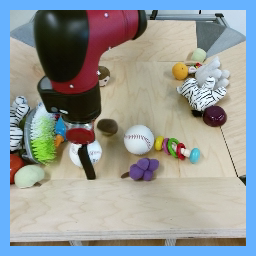 |
 |
 |
 |
 |
 |
 |
| Moving parts | ||||||||
| Kinetics | Whole frames |  |
 |
 |
 |
 |
 |
 |
| Moving parts | ||||||||
| AudioSet- Drums | Whole frames |  |
 |
 |
 |
 |
 |
 |
| Moving parts | ||||||||
| ∗: the pixel-wise distances are obtained by applying a factor (omitted for clarity). | ||||||||
Kinetics. CCVS ranks second on Kinetics video prediction benchmark. Kinetics contains more diversity than BAIR, and the reconstruction is thus more difficult. A solution [54] is to increase the codebook size (Table 7) but it stops translating into better prediction FVD at some point. We also try removing the quantization step (equivalent to an infinite codebook), and directly regressing latent features with (instead of ranking the likelihood of possible tokens). It allows better reconstructions, yet the prediction FVD is high. Figure 8 shows examples of synthetic continuations conditioned on 5-frame unseen test sequences. CCVS produces realistic and temporally coherent outputs which display various types of motion (e.g., body, hand, camera).
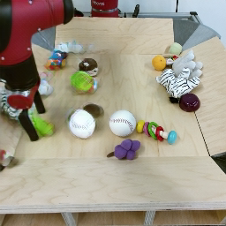
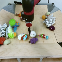
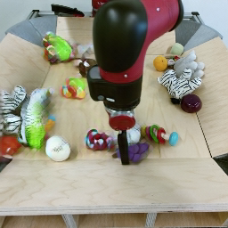
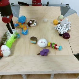
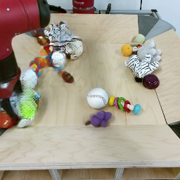
AudioSet-Drums. CCVS achieves top performance on sound-conditioned video synthesis on AudioSet Drums (Table 3). Figure 9 shows quantitative and qualitative insights on the diversity of the synthetic trajectories conditioned on the same input for the three datasets. The diversity metrics (DIV) computed on whole frames is lower on AudioSet Drums than on the other two datasets. This is explained by the fact that motion is quite repetitive and involves a limited portion of the frame. The same metric on moving parts only, and the end position of the drummer’s hand and upper left cymbal in qualitative samples, show the diversity of synthetic trajectories. An ablation of CCVS with/without audio guidance as well as more qualitative results on diversity can be found in Appendix E.
5 Discussion
CCVS is on par or better than the state-of-the-art on standard benchmarks, uses less computational resources, and scales to high resolution. Training neural networks is environmentally costly, due to the carbon footprint to power processing hardware [61, 17]. Methods sparing GPU-hours like ours are crucial to make AI less polluting [61, 43], and move from a “Red” to a “Green” AI [58]. Future work will include exploring new codebook strategies and synthesis guided by textual information.
Limitations.
CCVS uses a complex architecture and a two-stage training strategy. Simplification of both is an interesting direction for improving the method. Moreover, CCVS lacks global regularization of motion (flow computed on pairs of timesteps), and its efficiency relies on recycling context information such that synthesizing content from scratch (i.e., no input frame given) remains difficult.
Broader impact.
The increased accessibility and the many controls CCVS offers could accelerate the emergence of questionable applications, such as “deepfakes” (e.g., a video created from someone’s picture and an arbitrary audio) which could lead to harassment, defamation, or dissemination of fake news. On top of current efforts to automate their detection [49], it remains our responsibility to grow awareness of these possible misuses. Despite these worrying aspects, our contribution has plenty of positive applications which outweigh the potential ethical harms. Our efficient compression scheme is a step in the direction of real-time solutions: e.g., enhancing human-robot interactions, or improving the safety of self-driving cars by predicting the trajectories of people and vehicles nearby.
Acknowledgements
This work was granted access to the HPC resources of IDRIS under the allocation 2020-AD011012227 made by GENCI. It was funded in part by the French government under management of Agence Nationale de la Recherche as part of the “Investissements d’avenir” program, reference ANR-19-P3IA-0001 (PRAIRIE 3IA Institute). JP was supported in part by the Louis Vuitton/ENS chair in artificial intelligence and the Inria/NYU collaboration. We thank the reviewers for useful comments.
References
- [1] Dinesh Acharya, Zhiwu Huang, Danda Pani Paudel, and Luc Van Gool. Towards high resolution video generation with progressive growing of sliced wasserstein GANs. arXiv preprint, 2018.
- [2] Mohammad Babaeizadeh, Chelsea Finn, Dumitru Erhan, Roy H. Campbell, and Sergey Levine. Stochastic variational video prediction. In ICLR, 2018.
- [3] Yoshua Bengio, Nicholas Léonard, and Aaron C. Courville. Estimating or propagating gradients through stochastic neurons for conditional computation. arXiv preprint, 2013.
- [4] Tom Brown, Benjamin Mann, Nick Ryder, Melanie Subbiah, Jared D Kaplan, Prafulla Dhariwal, Arvind Neelakantan, Pranav Shyam, Girish Sastry, Amanda Askell, Sandhini Agarwal, Ariel Herbert-Voss, Gretchen Krueger, Tom Henighan, Rewon Child, Aditya Ramesh, Daniel Ziegler, Jeffrey Wu, Clemens Winter, Chris Hesse, Mark Chen, Eric Sigler, Mateusz Litwin, Scott Gray, Benjamin Chess, Jack Clark, Christopher Berner, Sam McCandlish, Alec Radford, Ilya Sutskever, and Dario Amodei. Language models are few-shot learners. In NeurIPS, 2020.
- [5] Joao Carreira, Eric Noland, Andras Banki-Horvath, Chloe Hillier, and Andrew Zisserman. A short note about Kinetics-600. arXiv preprint, 2018.
- [6] Joao Carreira and Andrew Zisserman. Quo vadis, action recognition? a new model and the kinetics dataset. In CVPR, 2017.
- [7] Lluis Castrejon, Nicolas Ballas, and Aaron Courville. Improved conditional VRNNs for video prediction. In ICCV, 2019.
- [8] Caroline Chan, Shiry Ginosar, Tinghui Zhou, and Alexei A. Efros. Everybody dance now. In ICCV, 2019.
- [9] Mark Chen, Alec Radford, Rewon Child, Jeffrey Wu, Heewoo Jun, David Luan, and Ilya Sutskever. Generative pretraining from pixels. In ICML, 2020.
- [10] Anoop Cherian, Moitreya Chatterjee, and Narendra Ahuja. Sound2Sight: Generating visual dynamics from sound and context. In ECCV, 2020.
- [11] Krzysztof Choromanski, Valerii Likhosherstov, David Dohan, Xingyou Song, Andreea Gane, Tamas Sarlos, Peter Hawkins, Jared Davis, Afroz Mohiuddin, Lukasz Kaiser, David Belanger, Lucy Colwell, and Adrian Weller. Rethinking attention with performers. In ICLR, 2021.
- [12] Aidan Clark, Jeff Donahue, and Karen Simonyan. Adversarial video generation on complex datasets. arXiv preprint, 2019.
- [13] Marius Cordts, Mohamed Omran, Sebastian Ramos, Timo Rehfeld, Markus Enzweiler, Rodrigo Benenson, Uwe Franke, Stefan Roth, and Bernt Schiele. The cityscapes dataset for semantic urban scene understanding. In CVPR, 2016.
- [14] Jia Deng, Wei Dong, Richard Socher, Li-Jia Li, Kai Li, and Li Fei-Fei. ImageNet: A large-scale hierarchical image database. In CVPR, 2009.
- [15] Emily Denton and Rob Fergus. Stochastic video generation with a learned prior. In ICML, 2018.
- [16] Jacob Devlin, Ming-Wei Chang, Kenton Lee, and Kristina Toutanova. BERT: Pre-training of deep bidirectional transformers for language understanding. In ACL, 2019.
- [17] Payal Dhar. The carbon impact of artificial intelligence. Nature Machine Intelligence, 2020.
- [18] Alexey Dosovitskiy, Lucas Beyer, Alexander Kolesnikov, Dirk Weissenborn, Xiaohua Zhai, Thomas Unterthiner, Mostafa Dehghani, Matthias Minderer, Georg Heigold, Sylvain Gelly, Jakob Uszkoreit, and Neil Houlsby. An image is worth 16x16 words: Transformers for image recognition at scale. In ICLR, 2021.
- [19] Frederik Ebert, Chelsea Finn, Alex X. Lee, and Sergey Levine. Self-supervised visual planning with temporal skip connections. In CoRL, 2017.
- [20] Patrick Esser, Robin Rombach, and Björn Ommer. Taming transformers for high-resolution image synthesis. In CVPR, 2021.
- [21] Chelsea Finn, Ian Goodfellow, and Sergey Levine. Unsupervised learning for physical interaction through video prediction. In NeurIPS, 2016.
- [22] Jean-Yves Franceschi, Edouard Delasalles, Mickaël Chen, Sylvain Lamprier, and Patrick Gallinari. Stochastic latent residual video prediction. In ICML, 2020.
- [23] Raghudeep Gadde, Varun Jampani, and Peter V. Gehler. Semantic video cnns through representation warping. In ICCV, 2017.
- [24] Hang Gao, Huazhe Xu, Qi-Zhi Cai, Ruth Wang, Fisher Yu, and Trevor Darrell. Disentangling propagation and generation for video prediction. In ICCV, 2019.
- [25] Jort F Gemmeke, Daniel PW Ellis, Dylan Freedman, Aren Jansen, Wade Lawrence, R Channing Moore, Manoj Plakal, and Marvin Ritter. Audio set: An ontology and human-labeled dataset for audio events. In ICASSP, 2017.
- [26] Ian Goodfellow, Jean Pouget-Abadie, Mehdi Mirza, Bing Xu, David Warde-Farley, Sherjil Ozair, Aaron Courville, and Yoshua Bengio. Generative adversarial nets. In NeurIPS, 2014.
- [27] Lena Gorelick, Moshe Blank, Eli Shechtman, Michal Irani, and Ronen Basri. Actions as space-time shapes. TPAMI, 2007.
- [28] Zekun Hao, Xun Huang, and Serge Belongie. Controllable video generation with sparse trajectories. In CVPR, 2018.
- [29] Kaiming He, Xiangyu Zhang, Shaoqing Ren, and Jian Sun. Deep residual learning for image recognition. In CVPR, 2016.
- [30] Ari Holtzman, Jan Buys, Li Du, Maxwell Forbes, and Yejin Choi. The curious case of neural text degeneration. In ICLR, 2020.
- [31] Cheng-Zhi Anna Huang, Ashish Vaswani, Jakob Uszkoreit, Ian Simon, Curtis Hawthorne, Noam Shazeer, Andrew M. Dai, Matthew D. Hoffman, Monica Dinculescu, and Douglas Eck. Music transformer. In ICLR, 2019.
- [32] Tak-Wai Hui, Xiaoou Tang, and Chen Change Loy. LiteFlowNet: A lightweight convolutional neural network for optical flow estimation. In CVPR, 2018.
- [33] Max Jaderberg, Karen Simonyan, Andrew Zisserman, and Koray Kavukcuoglu. Spatial transformer networks. In NeurIPS, 2015.
- [34] Amir Jamaludin, Joon Son Chung, and Andrew Zisserman. You said that?: Synthesising talking faces from audio. IJCV, 2019.
- [35] Rico Jonschkowski, Austin Stone, Jonathan T. Barron, Ariel Gordon, Kurt Konolige, and Anelia Angelova. What matters in unsupervised optical flow. In ECCV, 2020.
- [36] Emmanuel Kahembwe and Subramanian Ramamoorthy. Lower dimensional kernels for video discriminators. Neural Networks, 2020.
- [37] Andrej Karpathy, George Toderici, Sanketh Shetty, Thomas Leung, Rahul Sukthankar, and Li Fei-Fei. Large-scale video classification with convolutional neural networks. In CVPR, 2014.
- [38] Tero Karras, Samuli Laine, Miika Aittala, Janne Hellsten, Jaakko Lehtinen, and Timo Aila. Analyzing and improving the image quality of stylegan. In CVPR, 2020.
- [39] Angelos Katharopoulos, Apoorv Vyas, Nikolaos Pappas, and François Fleuret. Transformers are RNNs: Fast autoregressive transformers with linear attention. In ICML, 2020.
- [40] Will Kay, Joao Carreira, Karen Simonyan, Brian Zhang, Chloe Hillier, Sudheendra Vijayanarasimhan, Fabio Viola, Tim Green, Trevor Back, Paul Natsev, Mustafa Suleyman, and Andrew Zisserman. The kinetics human action video dataset. arXiv preprint, 2017.
- [41] Diederik P Kingma and Jimmy Ba. Adam: A method for stochastic optimization. In ICLR, 2015.
- [42] Manoj Kumar, Mohammad Babaeizadeh, Dumitru Erhan, Chelsea Finn, Sergey Levine, Laurent Dinh, and Durk Kingma. VideoFlow: A conditional flow-based model for stochastic video generation. In ICLR, 2020.
- [43] Alexandre Lacoste, Alexandra Luccioni, Victor Schmidt, and Thomas Dandres. Quantifying the carbon emissions of machine learning. In NeurIPS workshop, 2019.
- [44] Alex X. Lee, Richard Zhang, Frederik Ebert, Pieter Abbeel, Chelsea Finn, and Sergey Levine. Stochastic adversarial video prediction. arXiv preprint, 2018.
- [45] Pauline Luc, Aidan Clark, Sander Dieleman, Diego de Las Casas, Yotam Doron, Albin Cassirer, and Karen Simonyan. Transformation-based adversarial video prediction on large-scale data. arXiv preprint, 2020.
- [46] Arun Mallya, Ting-Chun Wang, Karan Sapra, and Ming-Yu Liu. World-consistent video-to-video synthesis. In ECCV, 2020.
- [47] Michael Mathieu, Camille Couprie, and Yann LeCun. Deep multi-scale video prediction beyond mean square error. In ICLR, 2016.
- [48] Willi Menapace, Stéphane Lathuilière, Sergey Tulyakov, Aliaksandr Siarohin, and Elisa Ricci. Playable video generation. In CVPR, 2021.
- [49] Thanh Thi Nguyen, Quoc Viet Hung Nguyen, Cuong M. Nguyen, Dung Nguyen, Duc Thanh Nguyen, and Saeid Nahavandi. Deep learning for deepfakes creation and detection: A survey. arXiv preprint, 2019.
- [50] Anselm Levskaya Nikita Kitaev, Lukasz Kaiser. Reformer: The efficient transformer. In ICLR, 2020.
- [51] Junting Pan, Chengyu Wang, Xu Jia, Jing Shao, Lu Sheng, Junjie Yan, and Xiaogang Wang. Video generation from single semantic label map. In CVPR, 2019.
- [52] Taesung Park, Ming-Yu Liu, Ting-Chun Wang, and Jun-Yan Zhu. Semantic image synthesis with spatially-adaptive normalization. In CVPR, 2019.
- [53] Ruslan Rakhimov, Denis Volkhonskiy, Alexey Artemov, Denis Zorin, and Evgeny Burnaev. Latent video transformer. arXiv preprint, 2020.
- [54] Aditya Ramesh, Mikhail Pavlov, Gabriel Goh, Scott Gray, Chelsea Voss, Alec Radford, Mark Chen, and Ilya Sutskever. Zero-shot text-to-image generation. In ICML, 2021.
- [55] Olaf Ronneberger, Philipp Fischer, and Thomas Brox. U-net: Convolutional networks for biomedical image segmentation. In MICCAI, 2015.
- [56] Masaki Saito, Eiichi Matsumoto, and Shunta Saito. Temporal generative adversarial nets with singular value clipping. In ICCV, 2017.
- [57] Masaki Saito, Shunta Saito, Masanori Koyama, and Sosuke Kobayashi. Train sparsely, generate densely: Memory-efficient unsupervised training of high-resolution temporal GAN. IJCV, 2020.
- [58] Roy Schwartz, Jesse Dodge, Noah A. Smith, and Oren Etzioni. Green AI. ACM, 2020.
- [59] Karen Simonyan and Andrew Zisserman. Very deep convolutional networks for large-scale image recognition. In ICLR, 2015.
- [60] Khurram Soomro, Amir Roshan Zamir, and Mubarak Shah. UCF101: A dataset of 101 human actions classes from videos in the wild. arXiv preprint, 2012.
- [61] Emma Strubell, Ananya Ganesh, and Andrew McCallum. Energy and policy considerations for deep learning in NLP. In ACL, 2019.
- [62] Andrew Tao, Karan Sapra, and Bryan Catanzaro. Hierarchical multi-scale attention for semantic segmentation. arXiv preprint, 2020.
- [63] Yu Tian, Jian Ren, Menglei Chai, Kyle Olszewski, Xi Peng, Dimitris N. Metaxas, and Sergey Tulyakov. A good image generator is what you need for high-resolution video synthesis. In ICLR, 2021.
- [64] Du Tran, Lubomir Bourdev, Rob Fergus, Lorenzo Torresani, , and Manohar Paluri. Learning spatiotemporal features with 3d convolutional networks. In ICCV, 2015.
- [65] Sergey Tulyakov, Ming-Yu Liu, Xiaodong Yang, and Jan Kautz. MoCoGAN: Decomposing motion and content for video generation. In CVPR, 2018.
- [66] Thomas Unterthiner, Sjoerd van Steenkiste, Karol Kurach, Raphael Marinier, Marcin Michalski, and Sylvain Gelly. Towards accurate generative models of video: A new metric & challenges. arXiv preprint, 2018.
- [67] Aaron van den Oord, Oriol Vinyals, and Koray Kavukcuoglu. Neural discrete representation learning. In NeurIPS, 2017.
- [68] Ashish Vaswani, Noam Shazeer, Niki Parmar, Jakob Uszkoreit, Llion Jones, Aidan N. Gomez, Lukasz Kaiser, and Illia Polosukhin. Attention is all you need. In NeurIPS, 2017.
- [69] Ruben Villegas, Jimei Yang, Seunghoon Hong, Xunyu Lin, and Honglak Lee. Decomposing motion and content for natural video sequence prediction. In ICLR, 2017.
- [70] Carl Vondrick, Hamed Pirsiavash, and Antonio Torralba. Anticipating visual representations from unlabeled video. In CVPR, 2016.
- [71] Carl Vondrick, Hamed Pirsiavash, and Antonio Torralba. Generating videos with scene dynamics. In NeurIPS, 2016.
- [72] Carl Vondrick and Antonio Torralba. Generating the future with adversarial transformers. In CVPR, 2017.
- [73] Konstantinos Vougioukas, Stavros Petridis, and Maja Pantic. End-to-end speech-driven facial animation with temporal GANs. In BMVC, 2018.
- [74] Ting-Chun Wang, Ming-Yu Liu, Jun-Yan Zhu, Guilin Liu, Andrew Tao, Jan Kautz, and Bryan Catanzaro. Video-to-video synthesis. In NeurIPS, 2018.
- [75] Tsun-Hsuan Wang, Yen-Chi Cheng, Chieh Hubert Lin, Hwann-Tzong Chen, and Min Sun. Point-to-point video generation. In ICCV, 2019.
- [76] Yaohui Wang, Piotr Bilinski, Francois Bremond, and Antitza Dantcheva. G3AN: Disentangling appearance and motion for video generation. In CVPR, 2020.
- [77] Zhou Wang, Alan C. Bovik, Hamid R. Sheikh, and Eero P. Simoncelli. Image quality assessment: from error visibility to structural similarity. TIP, 2004.
- [78] Yuxiang Wei, Ming Liu, Haolin Wang, Ruifeng Zhu, Guosheng Hu, and Wangmeng Zuo. Learning flow-based feature warping for face frontalization with illumination inconsistent supervision. In ECCV, 2020.
- [79] Dirk Weissenborn, Oscar Täckström, and Jakob Uszkoreit. Scaling autoregressive video models. In ICLR, 2020.
- [80] Bohan Wu, Suraj Nair, Roberto Martin-Martin, Li Fei-Fei, and Chelsea Finn. Greedy hierarchical variational autoencoders for large-scale video prediction. In CVPR, 2021.
- [81] Yue Wu, Rongrong Gao, Jaesik Park, and Qifeng Chen. Future video synthesis with object motion prediction. In CVPR, 2020.
- [82] Dingdong Yang, Seunghoon Hong, Yunseok Jang, Tianchen Zhao, and Honglak Lee. Diversity-sensitive conditional generative adversarial networks. In ICLR, 2019.
- [83] Yasin Yaz, Chuan-Sheng Foo, Stefan Winkler, Kim-Hui Yap, Georgios Piliouras, and Vijay Chandrasekhar. The unusual effectiveness of averaging in GAN training. In ICLR, 2019.
Appendix A Detailed architecture design
 |
 |
| (1) Conversion from image to feature space () and vice versa (). In the later case, context frames help producing new ones via . | (2) Computations in at one resolution level. |
We describe the implementation choices for the different functional blocks which compose CCVS. Note that different parts of the framework may benefit from future advances in various research areas: autoregressive modeling, image synthesis, codebook learning and optical flow estimation for transformer , decoder , quantizer and flow module respectively.
Encoder and decoder.
Both the encoder and the decoder , illustrated in Figure A1-(1), use a sequence of modules handling information at different intermediate resolution levels (with reverse ordering from to ). Each module is implemented by a residual block [29] which increases or decreases the spatial resolution by a factor . In practice, we use the succession of two 2D convolutions with LeakyReLU activations and a skip connection in the form of a convolution.
Flow module.
The flow module , also illustrated in Figure A1-(1), allows the sharing of information between the encoding and decoding stages across different timesteps. Computations for one resolution level are detailed in Figure A1-(2): The “match” operation computes the correlation between features in and its closest spatial neighbours in . We thus obtain a 3D cost volume of size , where is the number of neighbours considered and is the spatial resolution. We apply 2D convolutions to this cost volume to deduce the residual flow and mask. The “refine” operation is also a residual update of and . It is made of 2D convolutions and takes as input the concatenation of features, mask and flow. Finally, the “fuse” operation update features from with information from the context in according to the update rule given in Figure A1-(1) and detailed in Section 3.2. For these operations, we take our inspiration from LiteFlowNet [32] which we adapt to handle not only the optical flow but also the proposed fusion mask. An extension to multi-frame context for this temporal skip connection mechanism is proposed in Appendix D.
Image and temporal discriminators.
The architecture of the image discriminator is similar to that of StyleGAN2 [38], and the temporal discriminator is essentially the same, with 3D instead of 2D convolutions to account for the temporal dimension. To avoid the propagation of errors when decoding frames autoregressively during inference (see the “shift-and-add” module introduced for this purpose in Figure 1), we mimic this iterative process at train time: decode frames one by one, then encode them back to obtain context features for the next steps. The resulting synthetic videos are fed to . To avoid excessive memory consumption due to the recursive encoding / decoding operations, we only keep the gradients for the context features from the immediate preceding frame.
Quantizer.
The implementation of the quantizer is straightforward since it is just using a codebook of learnable embeddings. Yet, the non-differentiable nature of this operation prevents gradients from training losses (introduced in Section 3.2) to backpropagate through and , and from to at the compression bottleneck. To solve this in practice, we use a straight-through gradient estimator [3] which ignores the quantization step during backward-pass.
Transformer.
The transformer is described in Section 3.3. Its input is obtained by transforming a sequence of tokens into a 2D matrix of size . For that, associates with each possible token and each of the positions in the sequence a learnable embedding of size . To leverage the prior information that successive fixed-sized portions of the sequence represent annotated frames, we propose a spatio-temporal decomposition of the positional embeddings with a term indicating the timestep, and another one indicating the position within the frame-related portion. This is illustrated in Figure 2. The input matrix is computed by adding the token embedding and the positional embedding for each token of the sequence. thus consists in the succession of multi-head self-attention layers, and position-wise fully connected layers.
Position estimator.
In the experiments (Section 4), we mention that we manually annotated the location of the robotic arm (more precisely, its gripper) in 500 frames of the BAIR dataset. We use these to train a position estimator so that we can extract the trajectory of the arm from any new video (and use this trajectory to guide the state-conditioned synthesis of new videos). To facilitate training and accelerate inference, we design our position estimator to exploit latent features (obtained from images with ) and to map them to the position of the arm. We use a simple architecture with a few downsampling convolutional layers and a fully connected layer to output the estimated position. The position estimator is trained by regressing the target 2D coordinates by minimizing the corresponding mean squared error.
Sound autoencoder.
To allow multimodal synthesis of video and sound, we first compute the short-time Fourier transform (STFT) of the raw audio to obtain a time-frequency representation of the sound. We then employ an encoding / quantization / decoding strategy similar to that used to construct , and for video frames (without in this case) to reduce dimension and obtain corresponding tokens for audio. These tokens are used as frame-level annotations to guide the synthesis, just as in state-conditioned synthesis.
Appendix B Role of the flow module
Looking at Figure A1, one may wonder whether the flow module alone is sufficient for predicting features for future frames which would result in potentially being completely ignored. This would only apply if a frame was fully determined from the preceding one, yet, this is not the case due to the inherent stochastic nature of future prediction in the considered datasets. We have conducted a simple experiment to demonstrate that features are actually used and that they actively drive the dynamics of the scene: We have repeated the “reconstruction” experiment from Table 1 for which we compare the final model (last line) with an ablation with fixed (i.e., fixing for all predicted timesteps). Results are available in Table B1.
| FVD | PSNR | |
|---|---|---|
| Fixed | ||
| Dynamic |
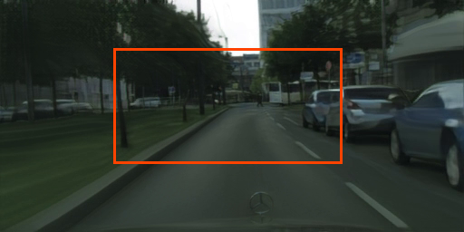
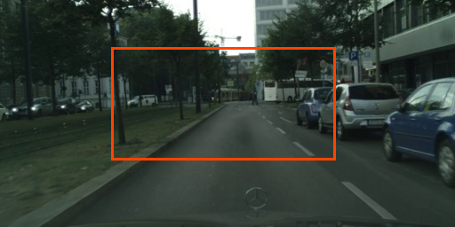
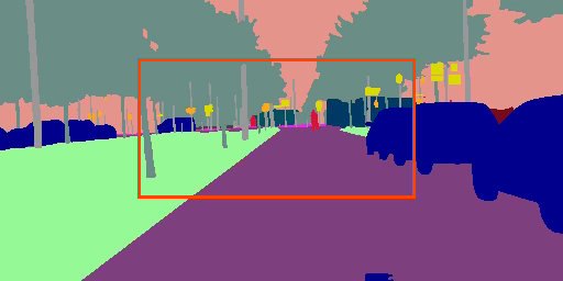
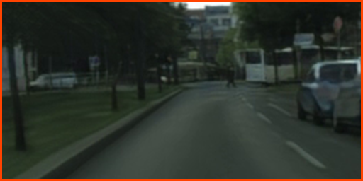
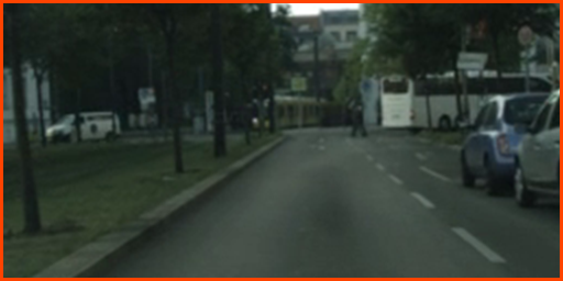
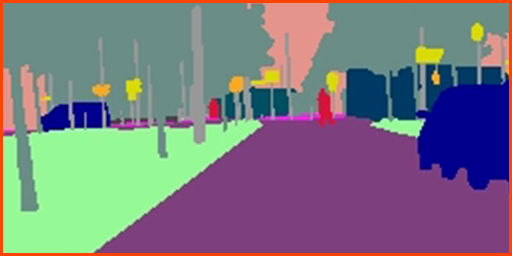
We observe that the reconstruction performance is much poorer when we force to remain constant for all timesteps. Qualitatively, looking at the synthesized videos, we see that they do not exhibit any motion, as one would expect when fixing the encoded features. Moreover, thanks to the fusion masks estimated by the flow module and used in Eq. (1), it is possible to observe how much information comes from and from respectively when generating . Figure F1 shows some examples of estimated masks on Cityscapes. Those are white when the source is , and black when it is context through . In practice, we see that they are white when the context is occluded and mostly grey in other regions. Thus, final videos are as much the result of context warping than direct decoding in non-occluded regions for this dataset. We observe similar behaviours on other datasets.
Appendix C Flow inversion approximation
For affine transformations, the exact inverse flow can be determined analytically. This is not the case for elastic deformations for which we propose to approximate this inverse flow from an input flow (where is the image spatial resolution). Here, maps cells from a grid to cells from the same grid (we ignore cells for which points out of the grid since they do not help in computing ). Such a mapping is not surjective, that is, all the cells in the grid are not necessarily reached. We compute the pixel-accurate inversion in cells for which there exists a direct mapping, and approximate others by iterative interpolation. That is, we keep track of inverted cells with a completion mask which we update with the closest cells in cardinal directions at every step. For the elastic deformations that we use when training CCVS, around 80% of the grid can be directly inverted in average, which is enough to accurately reconstruct the missing cells by interpolation.
The blurring function is a 2D convolution with Gaussian kernel (and -valued -sized padding to preserve the spatial resolution), and interpolates flow values from neighbouring cells weighted by the their proximity; Dilation function propagates -valued cells in a 2D boolean mask according to the cardinal directions (up, down, left, right); , and are notations which designate logical AND, OR and NOT respectively.
We note that an alternative to flow inversion is to use the flow module to compute the backward flow. This requires an extra forward pass in the flow module to compute both forward and backward flows and would result in additional GPU computations. Not to slow down training we prefer to run flow inversion on parallelized CPU processes as part of data loading. While both alternatives take approximately the same amount of time (0.15s on a GPU for backward flow estimation for a batch of 16 images at resolution , 0.12s on parallelized CPU for flow inversion for the same input) flow inversion is advantageous because, in our setup, GPU consumption is the limiting factor for speed (fully utilized GPUs, data loading on CPUs can run in the background).
Appendix D Extension of the flow module to multi-frame context
We extend the flow-module (introduced in Section 3.2) which aims at reusing contextual information from single- to multi-frame context. We thus consider a context consisting of frames. Just as before, for a given level and in , we use to compute the corresponding fusion mask and optical flow between intermediate encoded features (from context frame ) and the decoded features (that we wish to update). We recall that fusion masks handle occlusion by indicating for each spatial location the relevance of warped context features , that is, whether features correspond to at that location in terms of content, or not. Hence, we can derive from the fusion masks a confidence score defined as the context-wise normalization of features relevance, and use it to aggregate all the information that can be recovered from context by applying a weighted average: (9) where represents the element-wise division. In other words, given a spatial location, is an estimate for the likelihood that the content of matches any of the context frames, and is used to reconstruct this content faithfully by weighting proposals from the context by their relevance. This brings us back to the problem setup of Section 3.2, so that the aggregated fusion mask and warped features can be used to update , just as in single-frame fusion. The key benefits of this extension are the use of redundancy within context to better reconstruct the current frame, and the greater robustness to occlusion as different views are combined. This is demonstrated by the ablation study of the autoencoder in Table 1.
Appendix E Additional results
| Method | IS | FVD |
|---|---|---|
| StyleGAN2 [38] (repeat ) | ||
| Real frame (repeat ) | ||
| \hdashlineVGAN [71] | - | |
| TGAN [56] | - | |
| MoCoGAN [65] | - | |
| ProgressiveVGAN [1] | - | |
| LDVD-GAN [36] | - | |
| TGANv2 [57] | ||
| DVD-GAN [12] | - | |
| MoCoGAN-HD [63] | ||
| StyleGAN2 [38] + CCVS (ours) | ||
| \hdashlineReal frame + CCVS (ours) |
Unconditional synthesis.
We apply CCVS to unconditional video synthesis (i.e., the production of new videos without prior information about their content) on UCF-101 [60], an action-recognition dataset of categories for a total of approximately k video clips. Our approach leverages recent progress made in image synthesis by using StyleGAN2 [38] to produce the first frame. CCVS is able to improve over the state of the art on the FVD metric (computed on 2048 videos, under the same evaluation process as related approaches), but has an average performance () on the inception score (IS) [57] (computed on k videos, again with the appropriate protocol). IS measures the coverage of the different categories, and whether one of these is clearly identifiable in each of the synthetic videos, through the lens of the Softmax scores of a C3D network [64] trained for action recognition on the Sports-1M dataset [37] and fine-tuned on UCF-101. We also evaluate the performance of CCVS when considering a perfect image synthesizer (or one that has overfitted the training data) by using a real frame instead of a synthetic one to launch the prediction. This yields similar FVD but considerable improvements on IS (). Note that CCVS favorably contribute to IS in this setting because videos made from the same real frames (by repeating them along the temporal axis) have much lower IS (). A plausible explanation why MoCoGAN-HD [63] achieves a good IS score is due to it sampling multiple times from StyleGAN2 [38] (as opposed to once in our case, we use the same pretrained model). Indeed, MoCoGAN-HD synthesizes videos by finding a trajectory in the latent space of StyleGAN2. In this case, it may be easier to recognize a category because different modes can be interpolated (greater IS) but the outcome is less temporally realistic than ours (FVD near the one of still videos for MoCoGAN-HD). Future work will include trying to reconciliate both approaches.
Layout-conditioned synthesis.
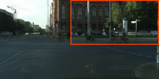
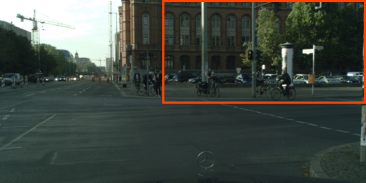
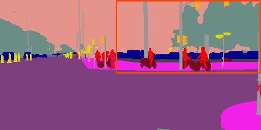
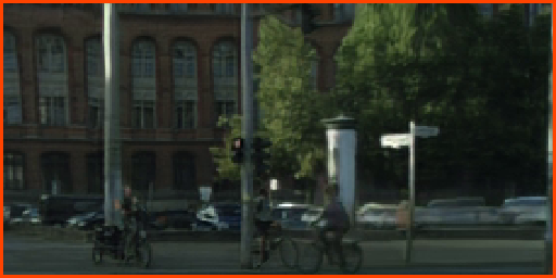
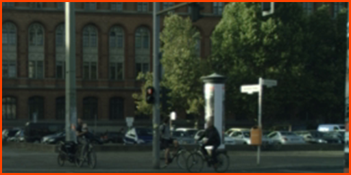
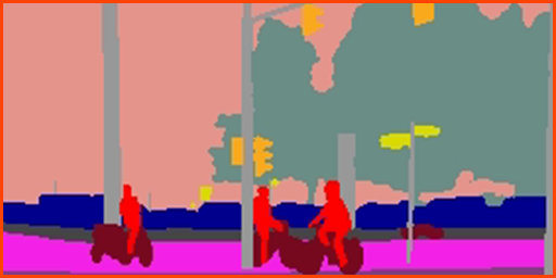
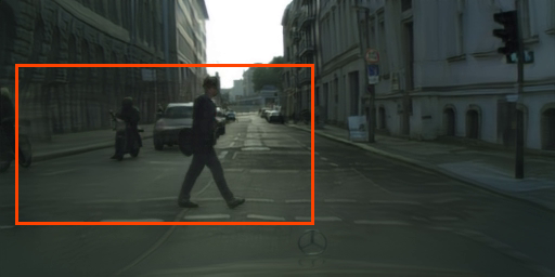
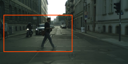
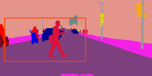
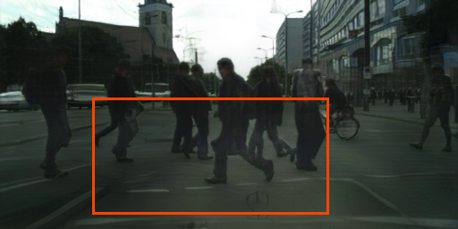
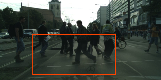
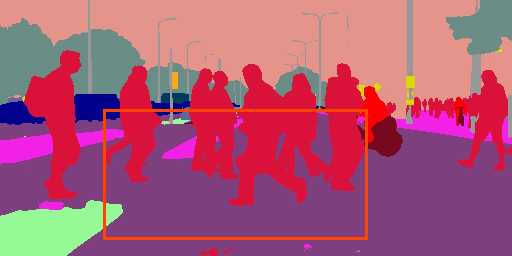
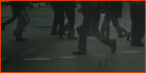
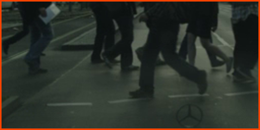
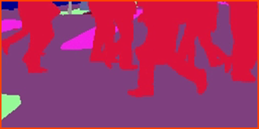
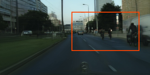
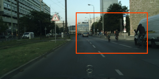
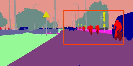
We explore here layout-conditioned synthesis where one controls the semantic structure of new frames by attributing a class to each of their spatial locations. To this end, we apply CCVS on image and layout sequence pairs on the Cityscapes dataset [13] which contains 3475 and 1525 30-frame sequences for train and test respectively. A single layout is annotated for each sequence, and we use a pretrained segmentation model [62] to obtain the remaining ones. Layouts are used as frame-level annotations for processing in . They are encoded, quantized, and decoded just as it is done for images. To save memory consumption during the decoding stage and ensure greater consistency between the two, frame and layout are decoded simultaneously with a single decoder (we just supplement with another prediction head to output layout masks). We show some qualitative results of CCVS on the synthesis of 30-frame videos given 3 starting frames and layouts for all timesteps in Figure D1. Synthetic videos closely follow the target semantic structure, remain temporally consistent, and can handle complex motions. We repeat this synthesis process in Figure D2, this time without layouts at subsequent timesteps. CCVS forecasts the semantic evolution of the scene on its own, predict corresponding layouts, and translate these into high-quality images. Both approaches (with or without layout at subsequent timesteps) are compared in Table D2. Having this additional information allows to produce videos which are closer to the real ones. A common architectural choice in layout-conditioned synthesis is to replace ResNet blocks [29] by SPADE blocks [52] to strengthen the layout guidance in the decoding stage [46]. Quantitatively, we see that it significantly improves the fidelity of the synthesized videos to the real ones in terms of SSIM and PSNR. Qualitatively, side-by-side reconstructions with and without SPADE in Figure D3 show that the flow module allows temporally consistent textures (similar to the 3D world model used in [46] but without being limited to static objects here) while SPADE enhances the compliance to the semantic structure, especially for small fast-moving objects.
| Layout |  |
 |
 |
 |
|
|---|---|---|---|---|---|
| Image |  |
 |
 |
 |
|
| Layout |  |
 |
 |
 |
|
| Image |  |
 |
 |
 |
|
| Layout |  |
 |
 |
 |
|
| Image |  |
 |
 |
 |
|
| Layout |  |
 |
 |
 |
|
| Image |  |
 |
 |
 |
|
| Layout |  |
 |
 |
 |
|
| Image |  |
 |
 |
 |
| Layout |  |
 |
 |
 |
|
|---|---|---|---|---|---|
| Image |  |
 |
 |
 |
|
| Layout |  |
 |
 |
 |
|
| Image |  |
 |
 |
 |
|
| Layout |  |
 |
 |
 |
|
| Image |  |
 |
 |
 |
|
| Layout |  |
 |
 |
 |
|
| Image |  |
 |
 |
 |
|
| Layout |  |
 |
 |
 |
|
| Image |  |
 |
 |
 |
| Method | Cond. | Layout | SSIM | PSNR | ||||
|---|---|---|---|---|---|---|---|---|
| CCVS (ours) | 3 | |||||||
| CCVS (ours) | 3 | ✓ | ||||||
| CCVS + [52] (ours) | 3 | ✓ | ||||||
| CCVS | CCVS + [52] | Real image | Real layout | ||
|---|---|---|---|---|---|
| Full | 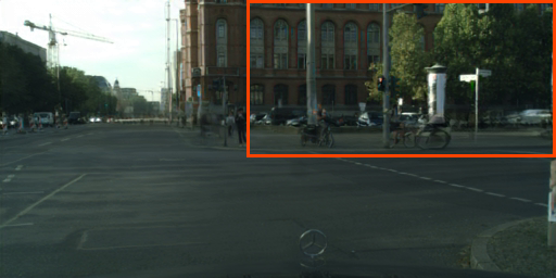 |
 |
 |
 |
|
| Zoom | 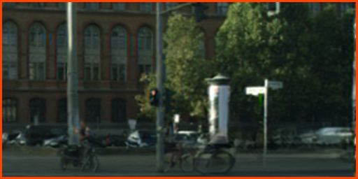 |
 |
 |
 |
|
| Full | 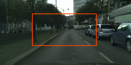 |
 |
 |
 |
|
| Zoom | 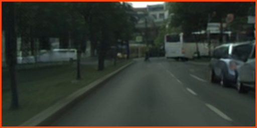 |
 |
 |
 |
|
| Full | 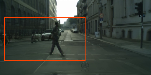 |
 |
 |
 |
|
| Zoom |  |
 |
 |
 |
|
| Full | 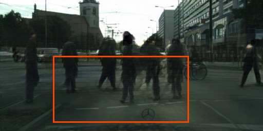 |
 |
 |
 |
|
| Zoom | 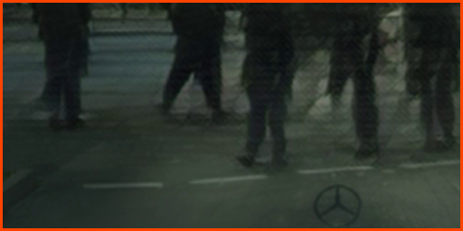 |
 |
 |
 |
|
| Full | 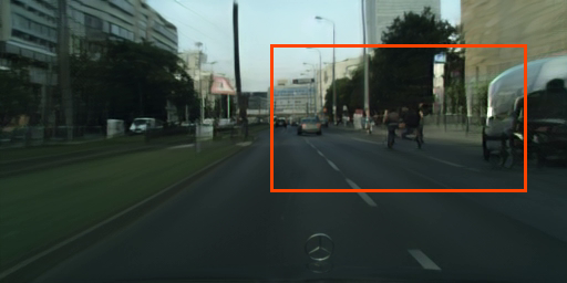 |
 |
 |
 |
|
| Zoom |  |
 |
 |
 |
Sound ablation study.
A simple ablation of CCVS on AudioSet Drum [25] is presented in Table D3. It shows that, as time goes by, the performance gap between unimodal and multimodal synthesis (when considering audio) increases. However, the improvement on account of the audio information seems relatively small compared to the overall performance. We suspect this is due to a minor part of the scene being animated (the drummer upper body) and to relatively fast motion (it is difficult to strictly minimize the image-to-image error between real and synthetic videos in this case).
| Method | Cond. | Audio | SSIM | PSNR | ||||
|---|---|---|---|---|---|---|---|---|
| CCVS (ours) | 1 | |||||||
| CCVS (ours) | 1 | ✓ | ||||||
Point-to-point synthesis.
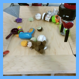
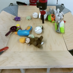
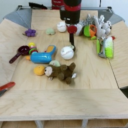
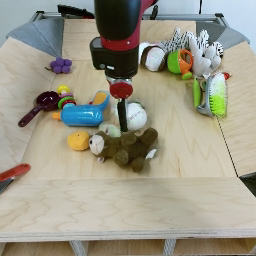
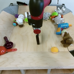
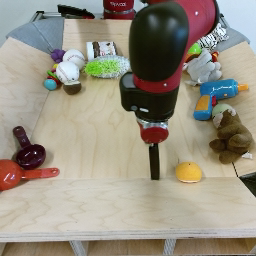
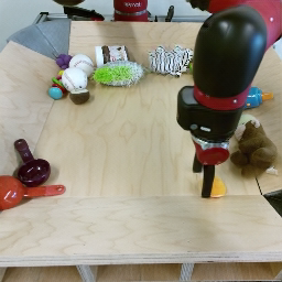
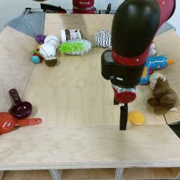
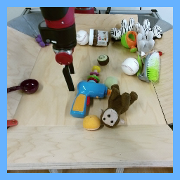
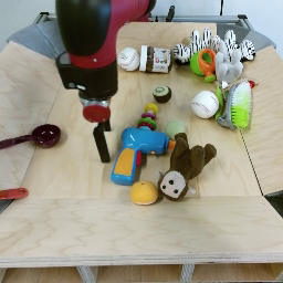
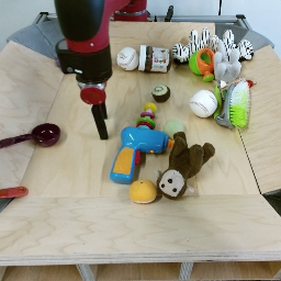
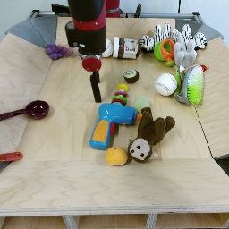
We explore further the performance of CCVS on the point-to-point synthesis task which we introduced in Section 4 of the article. We show some quantitative results against different baselines in Table D4. CCVS is on par or significantly outperforms the state of the art on out of metrics. It produces more faithful reconstructions when latent features are known. CCVS is more likely to synthesize the true outcome among predicted samples compared to baselines. It has a good control point consistency (i.e., the last synthetic frame is close to the corresponding ground-truth), but lower diversity than prior arts. We note, however, that SSIM diversity may capture the capacity of producing different trajectories between start and end points, but may also increase due to visual quality degradations. Like previous works [75], CCVS is able to produce videos of arbitrary length between the target start and end frames. We recall that the end frame is used as a video-level annotation in the transformer model (Figure 2) so that it is taken into account when predicting frames at earlier timesteps. To allow any timestep for the end frame (possibly greater than the capacity of ), we make its positional embedding reflect the gap with current predicted frames. Namely, the positional embedding of the end frame is updated as the sliding window moves forward in time and gets closer to the end timestep. We show qualitative results for different video lengths in Figure D4.
| Method | Cond. | SSIM | |||
|---|---|---|---|---|---|
| Best | Div. (1E-3) | C.P.C. | Rec. | ||
| SVG [15] | 2 | ||||
| SV2P [2] | 2 | ||||
| P2PVG [75] | 2 | ||||
| CCVS (ours) | 2 | ||||
 |
 |
 |
 |
 |
|||
 |
 |
 |
 |
 |
 |
||
 |
 |
 |
 |
 |
 |
 |
|
 |
 |
 |
 |
 |
|||
 |
 |
 |
 |
 |
 |
||
 |
 |
 |
 |
 |
 |
 |
|
 |
 |
 |
 |
 |
|||
 |
 |
 |
 |
 |
 |
||
 |
 |
 |
 |
 |
 |
 |
Class-conditioned synthesis.
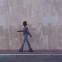
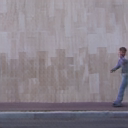
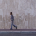
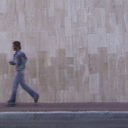
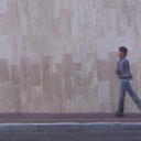
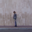
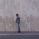
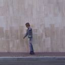
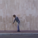
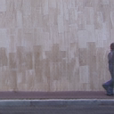
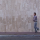
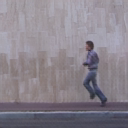
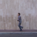
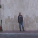
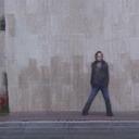
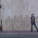
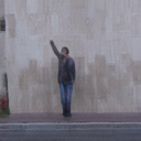
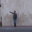
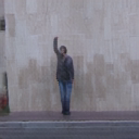
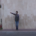
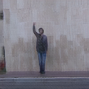
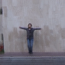
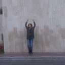
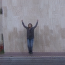
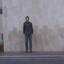
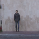
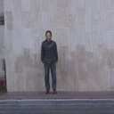
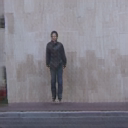
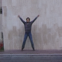
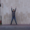
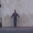
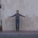
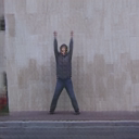
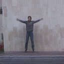
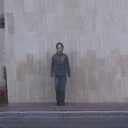
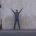
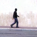
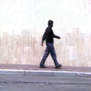
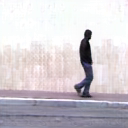
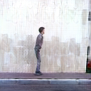
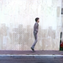
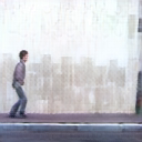
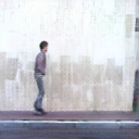
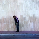
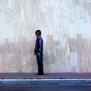
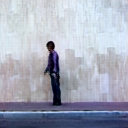
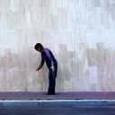
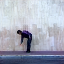
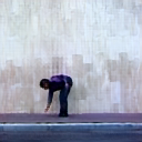
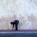
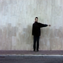
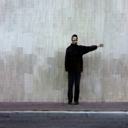
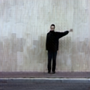
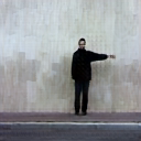
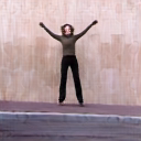
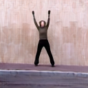
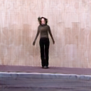
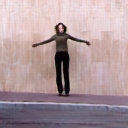
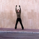
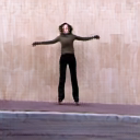
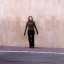
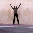
Next, we conduct a qualitative study of video synthesis conditioned on a class label on the Weizmann dataset [27], which consists of short clips captured from a fixed viewpoint from subjects, each performing the same actions. We use subjects for training and leave out for testing. CCVS tackles this task by specifying the class label as a video-level annotation in (Figure 2). We can make the held-out subject perform the learned actions accurately given a single input image (Table D5). Or we can synthesize new videos without any prior knowledge other than the desired class label (Table D6).
| walk | 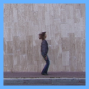 |
 |
 |
 |
 |
 |
 |
 |
 |
|---|---|---|---|---|---|---|---|---|---|
| run |  |
 |
 |
 |
 |
 |
 |
 |
 |
| jump |  |
 |
 |
 |
 |
 |
 |
 |
 |
| bend |  |
 |
 |
 |
 |
 |
 |
 |
 |
| skip |  |
 |
 |
 |
 |
 |
 |
 |
 |
| side | 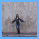 |
 |
 |
 |
 |
 |
 |
 |
 |
| wave1 |  |
 |
 |
 |
 |
 |
 |
 |
 |
| wave2 |  |
 |
 |
 |
 |
 |
 |
 |
 |
| pjump |  |
 |
 |
 |
 |
 |
 |
 |
 |
| jack |  |
 |
 |
 |
 |
 |
 |
 |
 |
| walk | 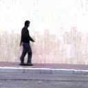 |
 |
 |
 |
 |
 |
 |
 |
 |
|---|---|---|---|---|---|---|---|---|---|
| run |  |
 |
 |
 |
 |
 |
 |
 |
 |
| jump | 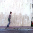 |
 |
 |
 |
 |
 |
 |
 |
 |
| bend | 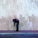 |
 |
 |
 |
 |
 |
 |
 |
 |
| skip |  |
 |
 |
 |
 |
 |
 |
 |
 |
| side |  |
 |
 |
 |
 |
 |
 |
 |
 |
| wave1 | 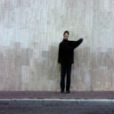 |
 |
 |
 |
 |
 |
 |
 |
 |
| wave2 | 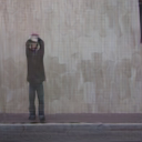 |
 |
 |
 |
 |
 |
 |
 |
 |
| pjump |  |
 |
 |
 |
 |
 |
 |
 |
 |
| jack | 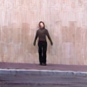 |
 |
 |
 |
 |
 |
 |
 |
 |
Qualitative ablation.
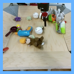
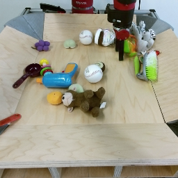
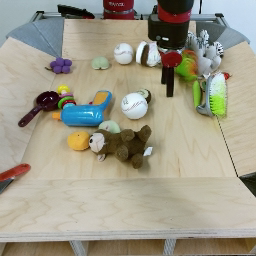
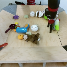
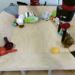
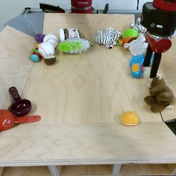
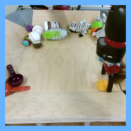
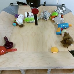
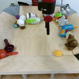
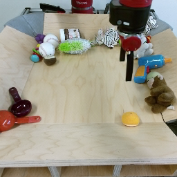
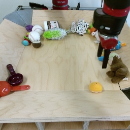
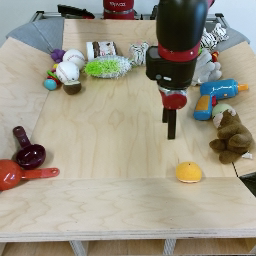
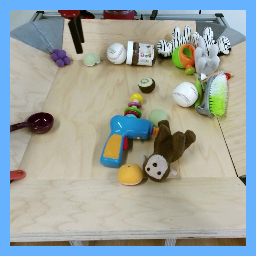
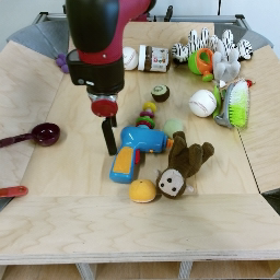
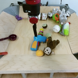
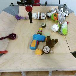
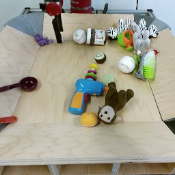
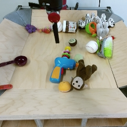
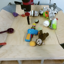
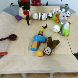
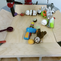
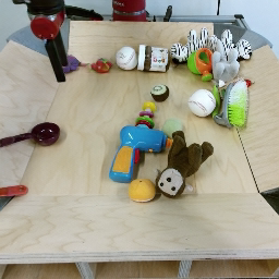
We repeat the ablation study of the autoencoder conducted in Table 1 on BAIR [19], by giving some qualitative samples of the reconstruction this time. The reconstruction results of 30-frame videos given the first frame and the compressed features at subsequent timesteps can be found in Table D5. To best compare different ablations of CCVS, we use the same input data for all. A model trained with the loss in RGB space reconstructs the static background and the robotic arm well, while other objects look very blurry. When using the same loss in the feature space of a net [59], objects display higher-frequency details, but look transparent. Having the image discriminator allows much more realistic outcomes, although these are still not temporally consistent, nor do they faithfully correspond to the ground-truth video. Having the temporal discriminator seems to improve over the temporal consistency issue. Thanks to the flow module , reconstructed videos are closer to the ground-truth ones, in particular at early timesteps. However, we see that flow imperfections cause synthesis artefacts which add up as time goes by, and result in quality degradation. The self-supervised technique used to learn mitigates this shortcoming. Finally, larger context windows and longer training times help to better recover details (see the more realistic texture and shape of manipulated objects for instance). The final proposal creates high-quality videos almost indistinguishable from real ones, and shows true interactions with objects (a ball and a colorful gun in this example). We see that in case of disocclusion (around the upper right corner is revealed), our model is able to synthesize plausible arrangements of objects despite lossy compression. These new objects remain consistent as the synthesis process unfolds (see ) thanks to the autoregressive nature of our approach.
| Self-recovery | Ctxt.-recovery | Reconstructed frames | ||||||||
| RGB | VGG | Sup. | Ctxt. | |||||||
| ✓ | 0 |
![[Uncaptioned image]](/html/2107.08037/assets/neurips2021/figures/sup/ablation-qualitative/rec/vid_00052_2.png)
|
![[Uncaptioned image]](/html/2107.08037/assets/neurips2021/figures/sup/ablation-qualitative/rec/vid_00052_10.png)
|
![[Uncaptioned image]](/html/2107.08037/assets/neurips2021/figures/sup/ablation-qualitative/rec/vid_00052_20.png)
|
![[Uncaptioned image]](/html/2107.08037/assets/neurips2021/figures/sup/ablation-qualitative/rec/vid_00052_30.png)
|
|||||
| [0pt][0pt] ✓ | ✓ | 0 |
![[Uncaptioned image]](/html/2107.08037/assets/neurips2021/figures/sup/ablation-qualitative/rec-vgg/vid_00052_2.png)
|
![[Uncaptioned image]](/html/2107.08037/assets/neurips2021/figures/sup/ablation-qualitative/rec-vgg/vid_00052_10.png)
|
![[Uncaptioned image]](/html/2107.08037/assets/neurips2021/figures/sup/ablation-qualitative/rec-vgg/vid_00052_20.png)
|
![[Uncaptioned image]](/html/2107.08037/assets/neurips2021/figures/sup/ablation-qualitative/rec-vgg/vid_00052_30.png)
|
||||
| ✓ | ✓ | ✓ | 0 |
![[Uncaptioned image]](/html/2107.08037/assets/neurips2021/figures/sup/ablation-qualitative/rec-vgg-adv/vid_00052_2.png)
|
![[Uncaptioned image]](/html/2107.08037/assets/neurips2021/figures/sup/ablation-qualitative/rec-vgg-adv/vid_00052_10.png)
|
![[Uncaptioned image]](/html/2107.08037/assets/neurips2021/figures/sup/ablation-qualitative/rec-vgg-adv/vid_00052_20.png)
|
![[Uncaptioned image]](/html/2107.08037/assets/neurips2021/figures/sup/ablation-qualitative/rec-vgg-adv/vid_00052_30.png)
|
|||
| [0pt][0pt] ✓ | ✓ | ✓ | ✓ | 0 |
![[Uncaptioned image]](/html/2107.08037/assets/neurips2021/figures/sup/ablation-qualitative/rec-vgg-adv-vid/vid_00052_2.png)
|
![[Uncaptioned image]](/html/2107.08037/assets/neurips2021/figures/sup/ablation-qualitative/rec-vgg-adv-vid/vid_00052_10.png)
|
![[Uncaptioned image]](/html/2107.08037/assets/neurips2021/figures/sup/ablation-qualitative/rec-vgg-adv-vid/vid_00052_20.png)
|
![[Uncaptioned image]](/html/2107.08037/assets/neurips2021/figures/sup/ablation-qualitative/rec-vgg-adv-vid/vid_00052_30.png)
|
||
| ✓ | ✓ | ✓ | ✓ | ✓ | 1 |
![[Uncaptioned image]](/html/2107.08037/assets/neurips2021/figures/sup/ablation-qualitative/rec-vgg-adv-vid-skip/vid_00052_2.png)
|
![[Uncaptioned image]](/html/2107.08037/assets/neurips2021/figures/sup/ablation-qualitative/rec-vgg-adv-vid-skip/vid_00052_10.png)
|
![[Uncaptioned image]](/html/2107.08037/assets/neurips2021/figures/sup/ablation-qualitative/rec-vgg-adv-vid-skip/vid_00052_20.png)
|
![[Uncaptioned image]](/html/2107.08037/assets/neurips2021/figures/sup/ablation-qualitative/rec-vgg-adv-vid-skip/vid_00052_30.png)
|
|
| [0pt][0pt] ✓ | ✓ | ✓ | ✓ | ✓ | ✓ | 1 |
![[Uncaptioned image]](/html/2107.08037/assets/neurips2021/figures/sup/ablation-qualitative/rec-vgg-adv-vid-skip-aug/vid_00052_2.png)
|
![[Uncaptioned image]](/html/2107.08037/assets/neurips2021/figures/sup/ablation-qualitative/rec-vgg-adv-vid-skip-aug/vid_00052_10.png)
|
![[Uncaptioned image]](/html/2107.08037/assets/neurips2021/figures/sup/ablation-qualitative/rec-vgg-adv-vid-skip-aug/vid_00052_20.png)
|
![[Uncaptioned image]](/html/2107.08037/assets/neurips2021/figures/sup/ablation-qualitative/rec-vgg-adv-vid-skip-aug/vid_00052_30.png)
|
| ✓ | ✓ | ✓ | ✓ | ✓ | ✓ | 8 |
![[Uncaptioned image]](/html/2107.08037/assets/neurips2021/figures/sup/ablation-qualitative/rec-vgg-adv-vid-skip-aug-8/vid_00052_2.png)
|
![[Uncaptioned image]](/html/2107.08037/assets/neurips2021/figures/sup/ablation-qualitative/rec-vgg-adv-vid-skip-aug-8/vid_00052_10.png)
|
![[Uncaptioned image]](/html/2107.08037/assets/neurips2021/figures/sup/ablation-qualitative/rec-vgg-adv-vid-skip-aug-8/vid_00052_20.png)
|
![[Uncaptioned image]](/html/2107.08037/assets/neurips2021/figures/sup/ablation-qualitative/rec-vgg-adv-vid-skip-aug-8/vid_00052_30.png)
|
| [0pt][0pt] ✓ | ✓ | ✓ | ✓ | ✓ | ✓ | 15 |
![[Uncaptioned image]](/html/2107.08037/assets/neurips2021/figures/sup/ablation-qualitative/rec-vgg-adv-vid-skip-aug-16/vid_00052_2.png)
|
![[Uncaptioned image]](/html/2107.08037/assets/neurips2021/figures/sup/ablation-qualitative/rec-vgg-adv-vid-skip-aug-16/vid_00052_10.png)
|
![[Uncaptioned image]](/html/2107.08037/assets/neurips2021/figures/sup/ablation-qualitative/rec-vgg-adv-vid-skip-aug-16/vid_00052_20.png)
|
![[Uncaptioned image]](/html/2107.08037/assets/neurips2021/figures/sup/ablation-qualitative/rec-vgg-adv-vid-skip-aug-16/vid_00052_30.png)
|
| Training longer (num. epochs ) |
![[Uncaptioned image]](/html/2107.08037/assets/neurips2021/figures/sup/ablation-qualitative/rec-vgg-adv-vid-skip-aug-16-more/vid_00052_2.png)
|
![[Uncaptioned image]](/html/2107.08037/assets/neurips2021/figures/sup/ablation-qualitative/rec-vgg-adv-vid-skip-aug-16-more/vid_00052_10.png)
|
![[Uncaptioned image]](/html/2107.08037/assets/neurips2021/figures/sup/ablation-qualitative/rec-vgg-adv-vid-skip-aug-16-more/vid_00052_20.png)
|
![[Uncaptioned image]](/html/2107.08037/assets/neurips2021/figures/sup/ablation-qualitative/rec-vgg-adv-vid-skip-aug-16-more/vid_00052_30.png)
|
||||||
| Oracle |
![[Uncaptioned image]](/html/2107.08037/assets/neurips2021/figures/sup/ablation-qualitative/real/vid_00052_2.png)
|
![[Uncaptioned image]](/html/2107.08037/assets/neurips2021/figures/sup/ablation-qualitative/real/vid_00052_10.png)
|
![[Uncaptioned image]](/html/2107.08037/assets/neurips2021/figures/sup/ablation-qualitative/real/vid_00052_20.png)
|
![[Uncaptioned image]](/html/2107.08037/assets/neurips2021/figures/sup/ablation-qualitative/real/vid_00052_30.png)
|
||||||
| “Sup.”: self-supervision of ; “Ctxt.”: number of context frames taken into account (in ) when decoding current frame (in ). | ||||||||||
Long-term synthesis.
We assess the ability of CCVS to generalize to long-term prediction through a qualitative study. We compare, for a model trained on sequences of length 16, the synthesis of 90-frame videos conditioned on a single frame and using different context windows for the flow module: 0 (not using the flow), 1, 4 and 16. Results on BAIR, Kinetics and AudioSet-Drums are available in Figure D7. When the flow is not used (size 0, i.e., a naïve extension of [20] or a setup close to [53]) videos are quite unstable and we see colors shifting over time. With a single-frame context window (size 1), there is a greater temporal consistency (e.g., the drum sticks are better preserved on AudioSet-Drums, the semantic structure shows higher fidelity to the input frame on BAIR or Kinetics), but in the long-term, synthesis artefacts add up due to the autoregressive decoding which leads to visual deterioration and saturation. These effects stand out the most on BAIR and Kinetics. The proposed multi-frame context extension (Appendix D) reduces this issue (size 4), and the latter becomes barely perceptible with an even larger context window (size 16). We found that even small context windows on AudioSet-Drums are sufficient thanks to the high inter-frame similarity.
| (a) BAIR (). | |||||||||
|---|---|---|---|---|---|---|---|---|---|
 |
 |
 |
 |
 |
 |
 |
 |
 |
|
 |
 |
 |
 |
 |
 |
 |
 |
 |
|
 |
 |
 |
 |
 |
 |
 |
 |
 |
|
 |
 |
 |
 |
 |
 |
 |
 |
 |
|
| (b) Kinetics (). | |||||||||
 |
 |
 |
 |
 |
 |
 |
 |
 |
|
 |
 |
 |
 |
 |
 |
 |
 |
 |
|
 |
 |
 |
 |
 |
 |
 |
 |
 |
|
 |
 |
 |
 |
 |
 |
 |
 |
 |
|
| (c) AudioSet-Drums (). | |||||||||
 |
 |
 |
 |
 |
 |
 |
 |
 |
|
 |
 |
 |
 |
 |
 |
 |
 |
 |
|
 |
 |
 |
 |
 |
 |
 |
 |
 |
|
 |
 |
 |
 |
 |
 |
 |
 |
 |
|
Appendix F Augmentation strategy
As discussed in Section 3.2, the self-supervision process used to train reconstructs a static image from both its latent representation and an augmented view as context by estimating the flow and mask corresponding to that augmentation. We illustrate this process on the Cityscapes dataset in Figure F1. We recall that, in this case, the context image can be writen as , where is an occlusion mask, and and some blurring and augmentation (i.e., spatial transformation) functions respectively. We can invert the flow corresponding to transformation thanks to Algorithm 1. The output corresponds to the target “Real Flow” in the illustration. As for the target “Real Mask”, it is obtained by warping the occlusion mask with the inverted flow. Looking at synthetic reconstructions, we see that visible details in the context are well recovered despite the augmentation. Indeed, real and synthetic flows match in non occluded areas (indicated by the dashed red line). Moreover, adversarial training produces high-quality images from blurred and occluded contexts. We notice that textures do not always match in real and synthetic images (e.g., building windows, car appearance). Yet, thanks to recovery losses, the semantic structure of the scene is preserved. Finally, we see that darker and lighter areas of the synthetic masks correspond to the same areas in the real ones. The darker the synthetic masks, the more features are updated from context. The whitish part indicates that in occluded areas the final image is reconstructed from its latent representation alone, and the greyish part shows that for other regions context is effectively reused (and latent representations still contribute to the final outcome). It is interesting to see that edges are visible in the synthetic masks. This indicates that those regions may be easier to detect (darker color) and play an important role in the image alignment process (estimation of the flow).
| Context | Image | Mask | Flow | ||
|---|---|---|---|---|---|
| Real | 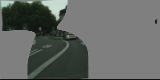 |
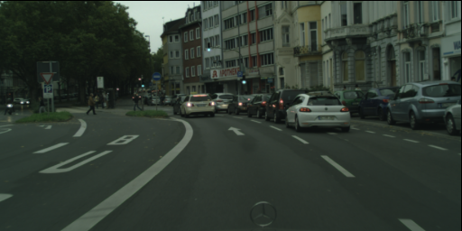 |
 |
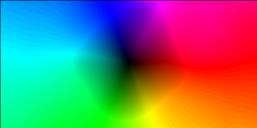 |
|
| Synthetic |  |
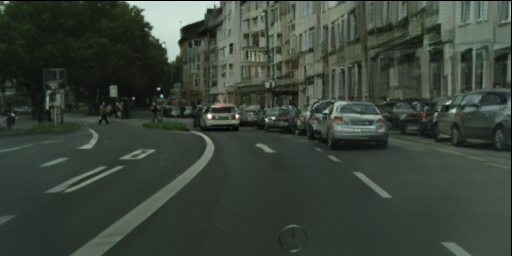 |
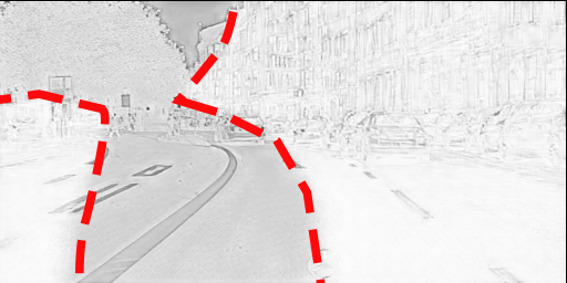 |
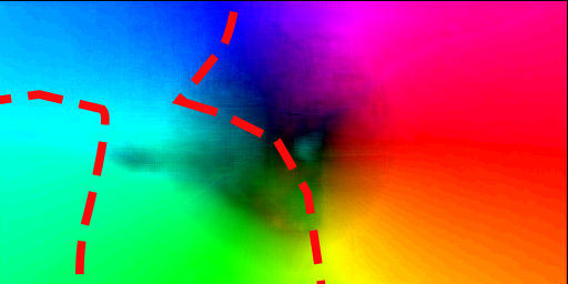 |
|
| Real |  |
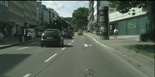 |
 |
 |
|
| Synthetic |  |
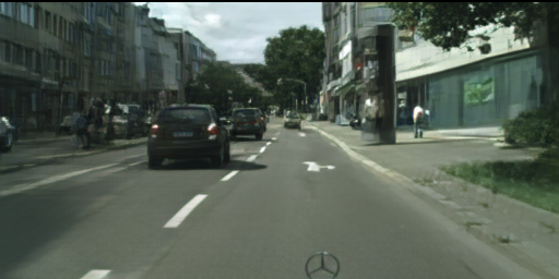 |
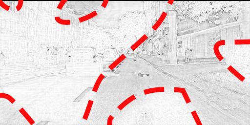 |
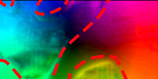 |
|
| Real |  |
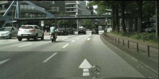 |
 |
 |
|
| Synthetic |  |
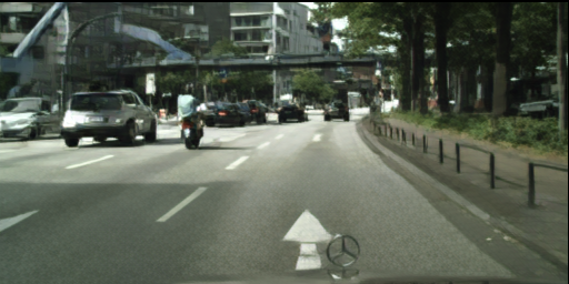 |
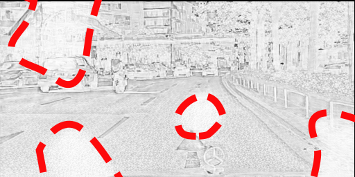 |
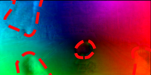 |