$H_{\infty}$ Inverse Optimal Attitude Tracking on the Special Orthogonal Group $SO(3)$

Abstract

The problem of attitude tracking using rotation matrices is addressed using an approach which combines inverse optimality and $\mathcal{L}_{2}$ disturbance attenuation. Conditions are provided which solve the inverse optimal nonlinear $H_{\infty}$ control problem by minimizing a meaningful cost function. The approach guarantees that the energy gain from an exogenous disturbance to a specified error signal respects a given upper bound. For numerical simulations, a simple problem setup from literature is considered and results demonstrate competitive performance.

1 Introduction

Rigid-body attitude control is an extensively studied control problem with numerous applications in aircraft, spacecraft, robotics, and marine systems. Different attitude parametrizations, or coordinates, have been used to develop a wide array of attitude control methods. Among these, the rotation matrix or direction cosine matrix (DCM), an element of the Special Orthogonal Group $SO\left(3\right)$, is the only attitude representation which is both globally defined and unique [1]. Other attitude representations either contain singularities (e.g., Euler angles) due to which they are not globally defined, or provide a non-unique attitude representation (e.g., quaternions) where two different coordinates describe the same attitude. In the case of quaternions, the resulting ambiguity in attitude representation can lead to unwinding [1].

Due to the limitations inherent to various attitude representations, several research efforts have sought to develop attitude controllers directly on the Special Orthogonal Group $SO(3)$. For the attitude tracking problem on $SO\left(3\right)$, a control design which has received significant attention is a simple PD-type controller, so named as it contains proportional and derivative-like terms representing the attitude and angular velocity errors, respectively (see [1, 2, 3] and the references therein). This controller has been shown to be almost semi-globally exponentially stabilizing [3, 4]. Moreover, for sufficiently large controller gains, the region of exponential convergence covers almost the entire state space. Given the simplicity and popularity of this controller, its disturbance rejection properties are of considerable interest.

The $\mathcal{L}_{2}$ disturbance attenuation framework, or nonlinear $H_{\infty}$ control, provides powerful tools for studying the disturbance rejection properties of feedback controllers (see [5, 6, 7]). In the case of state feedback, the approach facilitates the development of controllers which solve the suboptimal nonlinear $H_{\infty}$ problem, thereby ensuring that the energy gain from exogenous inputs, such as an external disturbance, to a specified error signal respects a given upper bound.

Several papers have considered the problem of $\mathcal{L}_{2}$ disturbance attenuation in the context of attitude control. In [8], a suboptimal nonlinear $H_{\infty}$ state feedback problem is formulated on $TSO\left(3\right)$, the tangent space of $SO\left(3\right)$, and addressed using a quaternion-PD controller. Quaternion-based $H_{\infty}$ control is also investigated in [9, 10] for state feedback controllers, and in [11] for PD control with delayed state measurements. In [12], $H_{\infty}$ attitude control is achieved with a state feedback controller using Modified Rodrigues Parameters (MRPs). For control laws defined on $SO\left(3\right)$, the suboptimal nonlinear $H_{\infty}$ problem is addressed in [2] for attitude errors smaller than $90\text{\textdegree}$.

A powerful approach to robust stabilization is obtained by combining the $\mathcal{L}_{2}$ disturbance attenuation framework with the inverse optimal control method [13, 14]. In the disturbance-free case, inverse optimal attitude control has been studied in [15] for the Cayley-Rodrigues parameters, and in [16] for exponential coordinates. For bounded disturbances, [17] uses the $H_{\infty}$ inverse optimal control method, described in [14], to establish the attitude tracking and $\mathcal{L}_{2}$ disturbance attenuation properties of a quaternion-PD state feedback controller. Building further on these ideas, [18] demonstrates the robustness of quaternion-based PD control to unmodeled actuator dynamics.

In this paper, we apply the inverse optimal $\mathcal{L}_{2}$ disturbance attenuation framework [14] to the problem of attitude tracking on $SO\left(3\right)$. In particular, we develop a state feedback controller directly on $SO\left(3\right)$ such that it solves the inverse optimal nonlinear $H_{\infty}$ problem almost globally (in the sense of [1]), thereby respecting a given upper bound on the energy gain from the disturbance to a specified error signal. The main contribution of this work is the provision of $H_{\infty}$ guarantees for a PD-type control law with scalar gains, at the cost of some mild constraints on the controller gains. We also demonstrate that the disturbance rejection properties of control laws (with scalar gains) synthesized using a common configuration error function on $SO(3)$, namely the chordal metric, tend to deteriorate for very large errors. This is due to the reduction in control effectiveness which has been observed in chordal metric-based control laws for very large errors, and which is known to cause arbitrarily slow convergence for errors close to $180\text{\textdegree}$ [1, 19].

The rest of the paper is organized as follows. Essential background on nonlinear $H_{\infty}$ control and an important result in $H_{\infty}$ inverse optimal control are summarized in Section 2, along with some remarks on the notation. The attitude control problem using rotation matrices is reviewed in Section 3, while the main results of this paper are presented in Section 4. In Section 5, a simple simulation setup is adapted from [17], and used to demonstrate the effectiveness of the proposed control law in tracking and disturbance attenuation. Finally, concluding remarks are given in the last section.

2 Preliminaries

Let us consider a general nonlinear system:

$$\dot{x} =f(x)+g_{1}(x)d+g_{2}(x)u, z =\begin{bmatrix}h(x)\\ \sqrt{r}u\end{bmatrix},$$ (2.1)

where $x$ is the state vector, $d$ is an exogenous disturbance, $u$ is the control input, $z$ is the penalized performance output signal, $h\left(x\right)$ is a positive state penalty, and $r$ is a positive scalar. We assume that the functions $f(x)$, $g_{1}(x)$, $g_{2}(x)$, and $h(x)$ are smooth, and the origin $x=0$ is an equilibrium point of (2.1), i.e., $f(0)=h(0)=0$. Also, the disturbance $d$ belongs to the set of bounded-energy signals, i.e., $\int_{0}^{T}\left|d(t)\right|^{2}dt<\infty$ for all finite $T\geq 0$.

2.1 Nonlinear $H_{\infty}$ Control

Definition 1 (Nonlinear $H_{\infty}$ control or $\mathcal{L}_{2}$-disturbance attenuation problem [7]).

The goal is to find a state feedback $u=k(x)$ such that $\forall$ $T\geq 0$, $x_{0}$, and $d(t)$, the $\mathcal{L}_{2}$ gain from the disturbance $d$ to the output signal $z(x,u)$ is less than or equal to $\gamma$. More precisely, for a positive function $S(x)\geq 0$,

$$\int_{0}^{T}\left|z\left(t\right)\right|^{2}dt\leq S(x_{0})+\gamma^{2}\int_{0}^{T}\left|d\left(t\right)\right|^{2}dt.$$ (2.2)

As has been well established in the literature on nonlinear $H_{\infty}$ control, the requirement (2.2) on the $\mathcal{L}_{2}$ gain is closely related to the notion of dissipativity. In particular, we seek a control law such that a smooth candidate storage function $V(x)\geq 0$, with $V(0)=0$, is dissipative with respect to a given supply rate $U\left(d,z\right)$, i.e., the following condition is satisfied:

$$\dot{V}\leq U.$$ (2.3)

Along trajectories of (2.1), we have that:

$$\dot{V}=V_{x}f+\left(V_{x}g_{1}\right)d+\left(V_{x}g_{2}\right)u,$$ (2.4)

where $V_{x}$ is a row vector of partial derivatives with respect to the state $x$. Consider the supply rate

$$U\left(d,z\right)=\frac{\gamma^{2}}{4}d^{\top}d-\frac{1}{4}z^{\top}z,$$

where $\gamma$ is a positive scalar. Substitute the penalized output signal $z$ and the supply rate in (2.3):

$$\dot{V}+\frac{1}{4}h^{\top}h+\frac{1}{4}ru^{\top}u-\frac{\gamma^{2}}{4}d^{\top}d\leq 0.$$ (2.5)

Then, using (2.4), the worst-case disturbance can be found as:

$$\left(V_{x}g_{1}\right)^{\top}-\frac{\gamma^{2}}{2}d^{*}=0\implies d^{*}=\frac{2}{\gamma^{2}}\left(V_{x}g_{1}\right)^{\top},$$ (2.6)

and the optimal state feedback is given by:

$$u(x)=-\frac{2}{r}\left(V_{x}g_{2}\right)^{\top}.$$ (2.7)

Substituting the worst-case disturbance $d^{*}$ and the above state feedback in (2.5), we arrive at the following expression for the dissipativity condition, known as the Hamilton-Jacobi-Isaacs (HJI) partial differential inequality:

$$V_{x}f-\frac{1}{r}\left|V_{x}g_{2}\right|^{2}+\frac{1}{\gamma^{2}}\left|V_{x}g_{1}\right|^{2}+\frac{1}{4}h^{\top}h\leq 0.$$ (2.8)

2.2 $H_{\infty}$ Inverse Optimal Control

A key step in solving the $H_{\infty}$ control problem involves finding a storage function such that the HJI inequality is satisfied. In situations where finding a suitable storage function isn’t easy, the dissipativity requirement can be addressed by invoking the notion of inverse optimality. In the $H_{\infty}$ inverse optimal method, the candidate storage function $V(x)$, re-interpreted as a candidate Lyapunov function, is used to obtain a constructive $H_{\infty}$ state-feedback control law. In particular, the inverse optimal approach constructs an optimal control problem, subject to the dynamics (2.1), whose value function is determined by the candidate Lyapunov function $V(x)$.

In the following, we state a simplified version of an important result on $H_{\infty}$ inverse optimal control. The result is from [14], and is used in [17] to obtain a quaternion-based nonlinear $H_{\infty}$ inverse optimal attitude tracking control law.

Lemma 2.

[14] Consider the nonlinear system (2.1), a candidate Lyapunov function $V\left(x\right)$, and the auxiliary system

$$\dot{x}=f(x)+\frac{1}{\gamma^{2}}g_{1}(x)\left(V_{x}g_{1}\right)^{\top}+g_{2}(x)u.$$ (2.9)

Suppose that the control law

$$u=\alpha(x)=-\frac{1}{r}\left(V_{x}g_{2}\right)^{\top}$$ (2.10)

globally asymptotically stabilizes (2.9) with respect to $V(x)$. Then the control law (2.7) solves the inverse optimal $H_{\infty}$ problem for (2.1) by minimizing the cost functional

$$J(u)=\sup_{d\in D}\bigg{(}\lim_{t\rightarrow\infty}\bigg{\{}4V(x(t))\\ +\int_{0}^{t}\left[l(x)+ru^{\top}u-\gamma^{2}d^{\top}d\right]d\tau\bigg{\}}\bigg{)},$$ (2.11)

where $D$ is the set of locally bounded functions of the state, and the state penalty is

$$l\left(x\right)=-4\left[V_{x}f-\frac{1}{r}\left|V_{x}g_{2}\right|^{2}+\frac{1}{\gamma^{2}}\left|V_{x}g_{1}\right|^{2}\right].$$ (2.12)

Furthermore, the value function of (2.11) is $4V\left(x\right)$, the optimal cost equals $J\left(u\right)=4V\left(x\left(0\right)\right)$, and the worst-case disturbance is given by (2.6). Lastly, the function $V\left(x\right)$ solves the following HJI equation:

$$V_{x}f-\frac{1}{r}\left|V_{x}g_{2}\right|^{2}+\frac{1}{\gamma^{2}}\left|V_{x}g_{1}\right|^{2}+\frac{l\left(x\right)}{4}=0,$$ (2.13)

and the achieved disturbance attenuation level is

$$\int_{0}^{\infty}\left[l\left(x\right)+ru^{\top}u\right]dt\leq\gamma^{2}\int_{0}^{\infty}\left\|d\right\|^{2}dt.$$ (2.14)

Remark 3.

We note that the $H_{\infty}$ inverse optimal state penalty $l\left(x\right)$ in (2.12) equals $-4\dot{V}_{\text{aux}}$, where

$$\dot{V}_{\text{aux}}=V_{x}f+\frac{1}{\gamma^{2}}\left|V_{x}g_{1}\right|^{2}-\frac{1}{r}\left|V_{x}g_{2}\right|^{2}$$

is the Lyapunov rate for the closed-loop auxiliary system (2.9)-(2.10). From the assumptions of the lemma, we know that $\dot{V}_{\text{aux}}<0$. As a result, $l\left(x\right)$ is positive definite, and the performance index in (2.11) is a meaningful cost, since it effectively penalizes the state and the control for each $\left(x,u\right)$ with a positive penality. Moreover, in the HJI equation (2.13), the state penalty $l\left(x\right)$ replaces the term $h^{\top}h$ in the HJI inequality (2.8). Thus, the $H_{\infty}$ inverse optimal method boils down to stabilizing the auxiliary system using the $\left(L_{g}V\right)$-type state-feedback (2.10). Note that the auxiliary term in (2.9) is also an $\left(L_{g}V\right)$-type term expressing the contribution of the worst-case disturbance to the HJI inequality (2.8).

2.3 Notation

The Special Orthogonal group $SO(3)$ is the set of $3\times 3$ orthogonal matrices with determinant $1$, i.e.,

$$SO(3) =\left\{R\in\mathbb{R}^{3\times 3}:R^{\top}R=I,\det\left(R\right)=1\right\}.$$

The hat map $\wedge:\mathbb{R}^{3}\rightarrow\mathfrak{so}(3)$ transforms a vector in $\mathbb{R}^{3}$ to a $3\times 3$ skew-symmetric matrix such that $\hat{x}y=x\times y$ for any $x,y\in\mathbb{R}^{3}$. Sometimes, $\hat{x}$ is written as $\left(x\right)^{\times}$ for clarity. In particular,

$$\hat{x}=\left(x\right)^{\times}=\begin{bmatrix}0&-x_{3}&x_{2}\\ x_{3}&0&-x_{1}\\ -x_{2}&x_{1}&0\end{bmatrix}.$$

The inverse of the hat map is denoted by the vee map $\vee:\mathfrak{so}(3)\rightarrow\mathbb{R}^{3}$. Finally, we recall some useful properties of the hat map [19]:

$$\hat{x}y =x\times y=-y\times x=-\hat{y}x,$$ (2.15)

$$x^{\top}\hat{x} =0,\quad\hat{x}=-\hat{x}^{\top},$$ (2.16)

$$\text{tr}\left[A\hat{x}\right] =\frac{1}{2}\text{tr}\left[\hat{x}\left(A-A^{\top}\right)\right]=-x^{\top}\left(A-A^{\top}\right)^{\vee},$$ (2.17)

$$\hat{x}A+A^{\top}\hat{x} =\left(\left\{\text{tr}[A]I-A\right\}x\right)^{\times},$$ (2.18)

$$R\hat{x}R^{\top} =\left(Rx\right)^{\times},$$ (2.19)

for any $x,y\in\mathbb{R}^{3}$, $A\in\mathbb{R}^{3\times 3}$, and $R\in SO(3)$.

3 Problem Formulation

The equations of motion for rigid-body rotation can be written as:

$$\begin{split}\dot{R}&=R\omega^{\times}\\ J\dot{\omega}&=-\omega^{\times}J\omega+\tau+d,\end{split}$$ (3.1)

where $R\in SO(3)$ is the rotation matrix, $\omega\in T_{I}SO(3)=\mathfrak{so}(3)$ is the angular velocity vector expressed in the body-fixed frame, $J$ is the moment of inertia matrix, $\tau$ is the net external torque, and $d$ is the disturbance torque. We are interested in tracking a given reference attitude which obeys the kinematics

$$\dot{R}_{d}=R_{d}\omega_{d}^{\times},$$ (3.2)

where the subscript in $R_{d}$ stands for ’desired’ or reference.

We define the right attitude error [4, pg. 554] as

$$R_{e}:=R_{d}^{\top}R\in SO(3).$$ (3.3)

Using (3.1)-(3.3) and the identity (2.19), the error kinematics can be expressed as

$$\dot{R}_{e} =R_{e}\left(\omega-R_{e}^{\top}\omega_{d}\right)^{\times}.$$

Next, we define the right angular velocity error as [4, pg. 555]:

$$\omega_{e}:=\omega-R_{e}^{\top}\omega_{d}.$$ (3.4)

Consequently, the error kinematics can be expressed as

$$\dot{R}_{e}=R_{e}\omega_{e}^{\times}.$$ (3.5)

Using (3.1) and (3.4)-(3.5), the error dynamics is given by:

$$J\dot{\omega}_{e} =J\dot{\omega}-JR_{e}^{\top}\dot{\omega}_{d}-J\dot{R}_{e}^{\top}\omega_{d}$$

$$=-\left(\omega_{e}+R_{e}^{\top}\omega_{d}\right)^{\times}J\left(\omega_{e}+R_{e}^{\top}\omega_{d}\right)+\tau+d$$

$$\begin{aligned} \quad\;&-JR_{e}^{\top}\dot{\omega}_{d}+J\omega_{e}^{\times}R_{e}^{\top}\omega_{d}\end{aligned}$$

Using identities (2.15) and (2.18) and some algebraic manipulation, three of the resulting terms can be simplified as follows:

$$-\omega_{e}^{\times}JR_{e}^{\top}\omega_{d}-\left(R_{e}^{\top}\omega_{d}\right)^{\times}J\omega_{e}+J\omega_{e}^{\times}R_{e}^{\top}\omega_{d}=-\omega_{e}^{\times}\bar{J}R_{e}^{\top}\omega_{d}$$

where $\bar{J}:=2J-\text{tr}[J]I$. Consequently, the error dynamics can be expressed as

$$J\dot{\omega}_{e}=-\omega_{e}^{\times}J\omega_{e}+\tau+d_{e},$$ (3.6)

where

$$d_{e}:=d-\omega_{e}^{\times}\bar{J}R_{e}^{\top}\omega_{d}-JR_{e}^{\top}\dot{\omega}_{d}-\left(R_{e}^{\top}\omega_{d}\right)^{\times}JR_{e}^{\top}\omega_{d}$$ (3.7)

includes the disturbance torque $d\left(t\right)$ as well as the terms containing the reference signals $\omega_{d}(t)$ and its time derivative $\dot{\omega}_{d}(t)$. Henceforth, the vector $d_{e}\left(t\right)$ is referred to as the extended disturbance.

The choice of configuration and velocity error functions is pivotal for control design on manifolds. We select the following configuration error function:

$$\Psi(R_{e}):=\frac{1}{2}\text{tr}\left[I-R_{e}\right].$$ (3.8)

From (3.5), the time derivative of $\Psi$ is given by

$$\dot{\Psi} =-\frac{1}{2}\text{tr}\left[\dot{R}_{e}\right]=-\frac{1}{2}\text{tr}\left[R_{e}\omega_{e}^{\times}\right]=\frac{1}{2}\left(R_{e}-R_{e}^{\top}\right)^{\vee}\cdot\omega_{e},$$

where the last equality follows from the identity (2.17). Define the configuration error vector as

$$e_{R}:=\frac{1}{2}\left(R_{e}-R_{e}^{\top}\right)^{\vee}.$$ (3.9)

Then, the rate of change of the configuration error function can be expressed as follows:

$$\dot{\Psi}=e_{R}\cdot\omega_{e}.$$ (3.10)

The time derivative of the configuration error vector can be obtained as follows:

$$\dot{e}_{R}^{\times} =\frac{1}{2}\left(\dot{R}_{e}-\dot{R}_{e}^{\top}\right)$$

$$=\frac{1}{2}\left(R_{e}\hat{\omega}_{e}+\hat{\omega}_{e}R_{e}^{\top}\right)$$

$$=\frac{1}{2}\left[\left(\text{tr}[R_{e}^{\top}]I-R_{e}^{\top}\right)\omega_{e}\right]^{\times}$$

$$\implies\dot{e}_{R} =\frac{1}{2}\left[\left(\text{tr}[R_{e}^{\top}]I-R_{e}^{\top}\right)\omega_{e}\right]$$ (3.11)

In the above simplification, the third line follows from the identity (2.18). Suppose that:

$$E(R_{e}):=\text{tr}[R_{e}^{\top}]I-R_{e}^{\top}.$$ (3.12)

Then, the time derivative of the configuration error vector can be expressed as follows:

$$\dot{e}_{R}=\frac{1}{2}E(R_{e})\omega_{e}.$$ (3.13)

Next, consider a control law of the form

$$\tau=u\left(e_{R},\omega_{e}\right)+u_{\text{FF}},$$ (3.14)

where $u\left(e_{R},\omega_{e}\right)\in\mathbb{R}^{3}$ is a feedback term, to be specified below, and

$$u_{\text{FF}}:=\omega_{e}^{\times}\bar{J}R_{e}^{\top}\omega_{d}+\left(R_{e}^{\top}\omega_{d}\right)^{\times}JR_{e}^{\top}\omega_{d}+JR_{e}^{\top}\dot{\omega}_{d}$$ (3.15)

is an optional feedforward compensation term which can be used to cancel the contribution of the terms in (3.7) which contain the reference angular velocity $\omega_{d}\left(t\right)$ or its time derivative $\dot{\omega}_{d}(t)$ . Consequently, from (3.6) and (3.13)-(3.14), with $u_{\text{FF}}=0$, the tracking error system with extended disturbance can be expressed as:

$$\begin{split}\dot{e}_{R}&=\frac{1}{2}E(R_{e})\omega_{e},\\ J\dot{\omega}_{e}&=-\omega_{e}^{\times}J\omega_{e}+u+d_{e}.\end{split}$$ (3.16)

Our goal is to find a feedback control law $u\left(e_{R},\omega_{e}\right)\in\mathbb{R}^{3}$ which achieves $H_{\infty}$ inverse optimal attitude tracking problem on $SO(3)$. In other words, we seek a stabilizing feedback control law which tracks the given reference signal ($R_{d},\omega_{d}$) while respecting a given upper bound on the energy gain from the extended disturbance $d_{e}$ to a linear combination of suitable state and input penalties, as in (2.14).

4 Robust Attitude Tracking on $SO(3)$

4.1 Candidate Storage Function

We consider the following candidate storage function:

$$V\left(R_{e},\omega_{e}\right):=\frac{a}{2}\omega_{e}\cdot J\omega_{e}+be_{R}\cdot J\omega_{e}+2c\Psi\left(R_{e}\right),$$ (4.1)

where $\omega_{e}$ is the angular velocity error (3.4), $\Psi$ is the configuration error function (3.8), $e_{R}$ is its associated configuration error vector (3.9), and $a,b,c$ are positive scalars. We note that the configuration error function is bounded as [3]:

$$\frac{1}{2}\left\|e_{R}\right\|^{2}\leq\Psi\left(R_{e}\right)\leq\frac{1}{2-\psi}\left\|e_{R}\right\|^{2},$$ (4.2)

where $\psi$ is a constant such that $0<\psi<2$, and the upper bound holds when $\Psi\left(R_{e}\right)\leq\psi.$ Using the lower bound, we obtain

$$V\geq\frac{1}{2}\begin{bmatrix}e_{R}\\ \omega_{e}\end{bmatrix}^{\top}\begin{bmatrix}2cI&bJ\\ bJ&aJ\end{bmatrix}\begin{bmatrix}e_{R}\\ \omega_{e}\end{bmatrix}.$$

Consequently, a sufficient condition for $V$ to be positive definite is given by

$$2acI>b^{2}J.$$ (4.3)

Using (3.10), we have that:

$$\dot{V} =a\omega_{e}\cdot J\dot{\omega}_{e}+b\dot{e}_{R}\cdot J\omega_{e}+be_{R}\cdot J\dot{\omega}_{e}+2c\dot{\Psi},$$

$$=\left(a\omega_{e}+be_{R}\right)\cdot J\dot{\omega}_{e}+b\dot{e}_{R}\cdot J\omega_{e}+2ce_{R}\cdot\omega_{e}.$$

Substituting the error dynamics from (3.16) and using the identity (2.16), it follows that:

$$\dot{V}=-be_{R}\cdot\omega_{e}^{\times}J\omega_{e}+b\dot{e}_{R}\cdot J\omega_{e}+2ce_{R}\cdot\omega_{e}\\ +\left(a\omega_{e}+be_{R}\right)\cdot\left(u+d_{e}\right).$$

We observe that:

$$e_{R}\cdot\omega_{e}^{\times}J\omega_{e}=-\omega_{e}^{\times}e_{R}\cdot J\omega_{e}=e_{R}^{\times}\omega_{e}\cdot J\omega_{e}$$

Therefore, from (3.9) and (3.11)-(3.12), it follows that:

$$\dot{e}_{R}-e_{R}^{\times}\omega_{e} =\frac{1}{2}\left(\left(\text{tr}[R_{e}^{\top}]I-R_{e}^{\top}\right)\omega_{e}-\left(R_{e}-R_{e}^{\top}\right)\omega_{e}\right)$$

$$=\frac{1}{2}\left(\text{tr}[R_{e}]I-R_{e}\right)\omega_{e}$$

$$=\frac{1}{2}E^{\top}(R_{e})\omega_{e}$$

Consequently, the rate of change of the storage function along trajectories of the error system (3.16) can be expressed as:

$$\dot{V}=\frac{b}{2}J\omega_{e}\cdot E^{\top}(R_{e})\omega_{e}+\left(a\omega_{e}+be_{R}\right)\cdot\left(u+d_{e}\right)\\ +2ce_{R}\cdot\omega_{e}$$ (4.4)

4.2 Auxiliary System

In this section, we use the storage function discussed above to study the robustness properties of the tracking error system (3.16). We employ the inverse optimal robust control approach, as summarized in Section 2. In particular, we consider an auxiliary system associated with (3.16), and establish its closed-loop stability under a PD-like feedback control law.

The auxiliary tracking error system is given as:

$$\begin{split}\dot{e}_{R}&=\frac{1}{2}E(R_{e})\omega_{e},\\ J\dot{\omega}_{e}&=-\omega_{e}^{\times}J\omega_{e}+u+\frac{1}{\gamma^{2}}\left(a\omega_{e}+be_{R}\right)\end{split}$$ (4.5)

It is seen that except for replacing the extended disturbance $d_{e}$ by the expression $\frac{1}{\gamma^{2}}\left(\omega_{e}+be_{R}\right)$, the auxiliary system is similar to the tracking error system (3.16).

We recall that due to a topological restriction, smooth control laws cannot achieve global stability in problems involving rotational degrees of freedom [20]. Therefore, we invoke standard notions of almost global asymptotic stability (AGAS) and almost semi-global exponential stability (AsGES) [1, 21] to prove the stability properties of the auxiliary system.

Theorem 4.

Consider the auxiliary tracking error system (4.5) and the control law

$$u=-\frac{1}{r}\left(a\omega_{e}+be_{R}\right).$$ (4.6)

Suppose the coefficients $a,b,c$ in the candidate Lyapunov function (4.1) and the scalars $\gamma$, $r$ satisfy the following conditions:

$$\gamma^{2} >r>0, c =ab\alpha, 0<b\lambda_{j}<a^{2}\alpha,$$ (4.7)

where $\lambda_{j}$ is the maximum eigenvalue of $J$, and

$$\alpha:=\frac{1}{r}-\frac{1}{\gamma^{2}}.$$ (4.8)

Then, the zero equilibrium $\left(e_{R},\omega_{e}\right)=\left(0,0\right)$ of (4.5) is almost globally asymptotically stable and almost semi-globally exponentially stable, i.e., the set of initial conditions for which exponential stability is guaranteed almost covers $SO\left(3\right)\times\mathbb{R}^{3}$ when $\alpha$ is sufficiently large:

$$\Psi\left(R_{e}\left(0\right)\right) \leq\psi<2$$

$$\left\|\omega_{e}\left(0\right)\right\|^{2} \leq\frac{2b\alpha}{\lambda_{j}}\left(\psi-\Psi\left(R_{e}\left(0\right)\right)\right).$$ (4.9)

Proof.

The proof uses several ideas discussed in [21], and is given in Appendix 7. ∎

4.3 $H_{\infty}$ Inverse Optimal Attitude Tracking

In this section, we build on earlier results in order to obtain a robust attitude tracking control law on $SO\left(3\right)$. In particular, we consider the tracking error system (3.16), and propose a state feedback which ensures $H_{\infty}$ inverse optimal attitude tracking with respect to the extended disturbance $d_{e}$ specified in (3.7).

We now state the main result concerning $H_{\infty}$ inverse optimal attitude tracking.

Theorem 5.

Consider the tracking error system (3.16), with the bounded extended disturbance $d_{e}$ defined as in (3.7). Consider also the inverse optimal $H_{\infty}$ control in which the objective is to minimize the cost functional

$$J_{a}(u)=\sup_{d\in D}\bigg{(}\lim_{t\rightarrow\infty}\bigg{\{}4V\left(R_{e},\omega_{e}\right)\\ +\int_{0}^{t}\left[l\left(R_{e},\omega_{e}\right)+ru^{\top}u-\gamma^{2}d_{e}^{\top}d_{e}\right]d\tau\bigg{\}}\bigg{)},$$ (4.10)

where $V\left(R_{e},\omega_{e}\right)$ is the candidate storage function (4.1), the state penalty function

$$l:=4a^{2}\alpha\left\|\omega_{e}\right\|^{2}+4b^{2}\alpha\left\|e_{R}\right\|^{2}-2bJ\omega_{e}\cdot E^{\top}\left(R_{e}\right)\omega_{e},$$ (4.11)

and $r>0$ is a scalar penalizing the control effort. Suppose that the coefficients $\alpha$, $a$, $b$, and $c$ in $V$ and $l$ satisfy the conditions (4.7)-(4.8) given in Theorem 4. Then:

1. $V$ and $l$ are nonnegative, and the state-feedback PD control

   $$u=-\frac{2}{r}\left(a\omega_{e}+be_{R}\right).$$ (4.12)

   solves the inverse optimal $H_{\infty}$ control problem for the closed-loop attitude tracking system (3.16) with respect to the performance index (4.10), where the worst-case extended disturbance $d_{e}$ is

   $$d_{e}^{*}=\frac{2}{\gamma^{2}}\left(a\omega_{e}+be_{R}\right).$$ (4.13)

2. The optimal cost is $J_{a}(u)=4V_{0}=4V(R_{e}(0),\omega_{e}(0))$, and the following disturbance attenuation level

   $$\int_{0}^{\infty}\left[l\left(R_{e},\omega_{e}\right)+ru^{\top}u\right]dt\leq\gamma^{2}\int_{0}^{\infty}\left\|d_{e}\right\|^{2}dt,$$

   is achieved.

Proof.

This theorem is a consequence of Lemma 2 and Theorem 4. In particular, we note the following correspondence between the terms in (2.4) and those in the Lyapunov rate (4.4) along trajectories of the tracking error system (3.16):

$$V_{x}f =\frac{b}{2}J\omega_{e}\cdot E^{\top}(R_{e})\omega_{e}+2ce_{R}\cdot\omega_{e}$$

$$V_{x}g_{1} =\left(a\omega_{e}+be_{R}\right)^{\top}$$

$$V_{x}g_{2} =\left(a\omega_{e}+be_{R}\right)^{\top}$$

Substituting these expressions in the state penalty (2.12) of Lemma 2, we obtain the following expression:

$$l\left(R_{e},\omega_{e}\right)=-4\left[\frac{b}{2}J\omega_{e}\cdot E^{\top}(R_{e})\omega_{e}+2ce_{R}\cdot\omega_{e}\right.\\ \left.-\left(\frac{1}{r}-\frac{1}{\gamma^{2}}\right)\left|a\omega_{e}+be_{R}\right|^{2}\right]$$

For the first claim, we note that Lemma 2 and the almost-global asymptotic stability of the auxiliary system (4.5), established in Theorem 4, directly imply that the control law (4.12) minimizes the cost functional (4.10) with the above state penalty. Moreover, substituting $c=ab\alpha$ from (4.7)-(4.8), we note that the state penalty can be re-stated as

$$l=4a^{2}\alpha\left\|\omega_{e}\right\|^{2}+4b^{2}\alpha\left\|e_{R}\right\|^{2}-2bJ\omega_{e}\cdot E^{\top}\left(R_{e}\right)\omega_{e}.$$

The second claim also follows from Lemma 2, and stipulates that the $\mathcal{L}_{2}$ gain from the extended disturbance $d_{e}$ to the tracking errors $\left(e_{R},\omega_{e}\right)$ and the control input $u$ is bounded by $\gamma$. ∎

Remark 6.

It is interesting to note that in both the state feedback (4.12) and the worst-case extended disturbance (4.13), the second term is proportional to the configuration error vector $e_{R}$. Recall that in terms of the axis-angle representation of the attitude error $R_{e}=R_{d}^{\top}R$, this vector can be expressed as $e_{R}=v\sin\theta_{e}$, where $v$ denotes the axis of rotation and $\theta_{e}$ the angle of rotation between the actual and desired orientations. Thus, we have that the proportional action of the controller and its disturbance rejection capability increase in the interval $\left|\theta_{e}\right|\in[0,\pi/2]$, and decrease to zero in the interval $\left|\theta_{e}\right|\in\left[\pi/2,\pi\right]$. This is an inherent limitation of PD controllers (with scalar gains) synthesised using the chordal metric (3.8), and is known to cause arbitrarily slow convergence for initial errors arbitrarily close to $180^{\circ}$ [19].

Remark 7.

The preceding results have been proven for a PD control law (3.14) without a feedforward term, but remain valid for a PD+ control law which uses feedforward compensation (3.15) to cancel the contribution of the reference-related terms in the error dynamics (3.6). This compensation requires accurate knowledge of the reference trajectory ($\omega_{d}$, $\dot{\omega}_{d}$) and the inertia properties of the rigid body. In general, this information is more likely to be available in spacecraft applications. If the reference or inertia properties are not accurately known, as is common for small rotorcraft and UAVs, then it might be better to avoid using the feedforward terms.

4.4 Tuning Guidelines

We recall the inverse optimal $H_{\infty}$ control law from (4.12):

$$u=-\frac{2}{r}\left(a\omega_{e}+be_{R}\right),$$

where the $a$, $b$, and $r$ are subject to the requirements given by (4.7), compactly written as

$$0<b\lambda_{j}<a^{2}\left(\frac{1}{r}-\frac{1}{\gamma^{2}}\right).$$ (4.14)

The PD parameters ($2b/r$, $2a/r$) can be chosen using any tuning method and then checked for the condition (4.14) which is quite easy to satisfy. Linearized model of the attitude dynamics can be especially helpful in fully exploiting the powerful frequency response methods and especially structured $H_{\infty}$ control design methods, see [22] for details. Once the linear design, having adequate performance and robustness properties, has been finalized, the condition (4.14) can be checked to guarantee almost-global disturbance rejection properties as stipulated in Theorem 5. If the condition (4.14) is not satisfied, one can reduce proportional action $b$ or increase derivative action $a$. Greater disturbance attenuation can be accomplished by decreasing $r$, thereby generating stronger control action. This highlights the trade off between disturbance rejection and control effectiveness.

5 Simulation Results

The results presented in section 4 may seem too technical to apply in practical problems, however, we illustrate through an example that nonlinear $H_{\infty}$ guarantees can be easily obtained for a control law design through standard (linear) control synthesis techniques.

We consider the attitude control problem of a small satellite and demonstrate a simple design approach leading to control laws with appealing performance. To this end, we consider the problem setup:

$$J=\text{diag}\left(10,10,8\right)\text{kg$\text{m}^{2}$},$$

$$d=\begin{bmatrix}0.005-0.05\sin(2\pi t/400)+\delta(200,0.2)+v_{1}\\ 0.005-0.05\sin(2\pi t/400)+\delta(250,0.2)+v_{2}\\ 0.005-0.03\sin(2\pi t/400)+\delta(300,0.2)+v_{3}\end{bmatrix},$$

where $v_{1}$, $v_{2}$, $v_{3}$ are the zero mean white Gaussian noises with variances $\sigma^{2}=0.015^{2}$. The desired angular velocity is:

$$\omega_{d}=\begin{bmatrix}0.05\sin(2\pi t/400)\\ -0.05\sin(2\pi t/400)\\ 0.03\sin(2\pi t/400)\end{bmatrix},$$

and the desired attitude kinematics ($\dot{R}_{d}=R_{d}\omega_{d}^{\times}$) is initialized with $R_{d}(0)=I$. The attitude dynamics is initialized with $\omega=(0,0,0)$ and rotation matrix equivalent of the quaternion $q(0)=\begin{bmatrix}0.3&0.2&0.3&-0.8832\end{bmatrix}^{\top}$. For direct comparison with a relevant result based on quaternions, this problem setup has been chosen as in [17], except for the variance of the white noises in $d$ which is taken higher for this paper.

For control synthesis, the decoupled single-axis model is considered and linearized around the origin. This simplified model, along with some nominal performance and robustness weights, is used to tune the (linear) structured $H_{\infty}$ controller via nonsmooth optimization techniques available in MATLAB. After some iterations of the algorithm, a linear control law meeting all the requirements on the single-axis linearized is found:

$$u=-\left(k_{P}\theta_{e}+k_{D}\omega_{e}\right),$$

$$k_{P} =0.9475, k_{D}=7.2836.$$

One could simply take the values of $k_{P}$, $k_{D}$ and check if the nonlinear control law

$$u=-k_{D}\omega_{e}+k_{P}e_{R},$$

would meet the requirements (4.14), where we have taken $k_{P}=\frac{2b}{r}e_{R}$, $k_{D}=\frac{2a}{r}\omega_{e}$ . It can be easily verified that the nonlinear controller, with $k_{P},k_{D}$ given above, meets the conditions (4.14) and therefore provides a nonlinear $H_{\infty}$ guarantee, i.e., the energy gain from extended disturbance to the tracking errors and control input is upper bounded by a finite constant $\gamma$.

The performance of the controller on both linearized single-axis model and full nonlinear $SO(3)$ model can be examined in the filtered-step response provided in Figure 5.1. Clearly, the response of linearized system with a linear controller is not the same as the fully nonlinear counterpart, however, the difference is not so great considering that the magnitude of the step input is 2 radians. Therefore, it may be useful to start the control design based on a linearized model (at least for a first-cut design) and then use this design to select the gains of the nonlinear system.

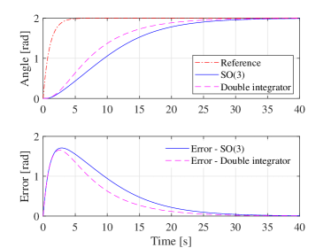
Figure 5.1: The filtered step reference of $2$ radians, and response on $SO(3)$ and the linearized single axis model.

The reference tracking capability of the proposed controller is evaluated on the problem setup given above. The reference attitude trajectory along with the achieved attitude is given in Figure 5.2. The error in attitude is plotted in terms of Euler angles and reported in Figure 5.3, with Euler rate errors in Figure 5.4. The components of control torque vector demanded by the proposed controller are shown in Figure 5.5.

The responses show adequate tracking and disturbance rejection properties and are no worse than those reported in literature for a quaternion based result [17].

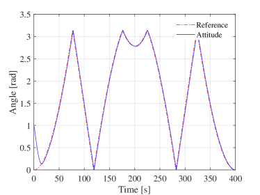
Figure 5.2: The plot of reference trajectory and actual attitude, in terms of angle or axis angle representation.

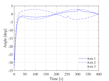
Figure 5.3: The plot of tracking error, in terms of three Euler angular errors.

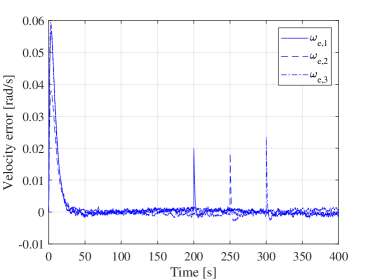
Figure 5.4: The plot of angular rate errors, in terms of Euler angle rates.

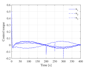
Figure 5.5: The plot of components of control torque vector demanded by the proposed control law.

6 Conclusion

The disturbance attenuation problem for the attitude tracking using rotation matrices has considered and addressed using an inverse optimal approach. It has been shown that the energy gain from disturbances to the tracking error is upper bounded by a given constant $\gamma$ if certain mild conditions on the controller gains are satisfied. A practical method for the tuning of controller gains has been illustrated using a numerical example, which draws on the powerful structured $H_{\infty}$ tuning method for the linearized single axis model. The proposed controller is found to exhibit competitive performance in the numerical simulations.

7 Proof of Theorem 4

Proof.

Replacing the disturbance $d_{e}$ in (4.4) by the term $\frac{1}{\gamma^{2}}\left(a\omega_{e}+be_{R}\right)$ and substituting the feedback law (4.6), the Lyapunov rate for the auxiliary system can be expressed as

$$\dot{V}_{\text{aux}}=\frac{b}{2}J\omega_{e}\cdot E^{\top}(R_{e})\omega_{e}-\left(\frac{1}{r}-\frac{1}{\gamma^{2}}\right)\left\|a\omega_{e}+be_{R}\right\|^{2}\\ +2ce_{R}\cdot\omega_{e}.$$

Expanding the second term, and using the expression for $\alpha$ in (4.8), the Lyapunov rate simplifies to

$$\dot{V}_{\text{aux}}=-a^{2}\alpha\left\|\omega_{e}\right\|^{2}-b^{2}\alpha\left\|e_{R}\right\|^{2}-2\left(ab\alpha-c\right)e_{R}\cdot\omega_{e}\\ +\frac{b}{2}J\omega_{e}\cdot E^{\top}(R_{e})\omega_{e}.$$

Using the MATLAB Symbolic Computation Tool, it can be shown that the matrix 2-norm of $E(R_{e})$ is

$$\left\|E\left(R_{e}\right)\right\|=2.$$

Therefore, choosing $c$ as in (4.7), the Lyapunov rate can be bounded as follows:

$$\dot{V}_{\text{aux}}\leq-a^{2}\alpha\left\|\omega_{e}\right\|^{2}-b^{2}\alpha\left\|e_{R}\right\|^{2}+b\lambda_{j}\left\|\omega_{e}\right\|^{2}$$

This can be expressed more compactly as

$$\dot{V}_{\text{aux}}\leq-x^{\top}M_{1}x,$$ (7.1)

where $x=\left[\left\|e_{R}\right\|,\left\|\omega_{e}\right\|\right]^{\top}$, and $M_{1}\in\mathbb{R}^{2\times 2}$ is given by

$$M_{1}:=\begin{bmatrix}b^{2}\alpha&0\\ 0&a^{2}\alpha-b\lambda_{j}\end{bmatrix}.$$ (7.2)

Therefore, the conditions on $a$, $b$ and $\alpha$, given in (4.7)-(4.8), ensure that $M_{1}$ is positive definite. In addition, these conditions also ensure that

$$2acI=2a^{2}b\alpha I>2b^{2}\lambda_{j}I>b^{2}J.$$

Consequently, the sufficient condition (4.3) for the positive-definiteness of $V$ is satisfied. This shows that the desired equilibrium of the auxiliary system (4.5) is asymptotically stable, and that $e_{R},\omega_{e}\rightarrow 0$ as $t\rightarrow\infty$.

Next, we show exponential stability. Define

$$U=\frac{a}{2}\omega_{e}\cdot J\omega_{e}+ab\alpha\Psi.$$

From (3.10), (4.5), (4.6), and (4.8), it follows that:

$$\dot{U} =a\omega_{e}\cdot J\dot{\omega}_{e}+ab\alpha e_{R}\cdot\omega_{e}$$

$$=a\omega_{e}\cdot\left(-\omega_{e}^{\times}J\omega_{e}-\alpha\left(a\omega_{e}+be_{R}\right)\right)+ab\alpha e_{R}\cdot\omega_{e}$$

$$=-a^{2}\alpha\left\|\omega_{e}\right\|^{2}$$

This implies that $U\left(t\right)$ is non-increasing. Therefore, for the set of initial conditions in (4.9), we obtain

$$\Psi\left(R_{e}\left(t\right)\right)\leq\frac{1}{ab\alpha}U\left(t\right) \leq\frac{1}{ab\alpha}U\left(0\right)$$

$$\leq\frac{\lambda_{j}}{2b\alpha}\left\|\omega_{e}\left(0\right)\right\|^{2}+\Psi\left(R_{e}\left(0\right)\right)$$

$$\leq\psi.$$

Thus, the upper bound in (4.2) is satisfied. Consequently, from (4.2) and (4.1), we have that

$$x^{\top}M_{2}x\leq V_{\text{aux}}\leq x^{\top}M_{3}x,$$ (7.3)

where $x=\left[e_{R}^{\top},\omega_{e}^{\top}\right]^{\top}$, and $M_{2},M_{3}\in\mathbb{R}^{6\times 6}$ are given by

$$M_{2} =\begin{bmatrix}2cI&bJ\\ bJ&aJ\end{bmatrix}, M_{3}= \begin{bmatrix}\frac{4c}{2-\psi}I&bJ\\ bJ&aJ\end{bmatrix}.$$

We have already seen that the conditions on $\alpha$, $a$, $b$, and $c$ in (4.7)-(4.8) ensure that $M_{2}$ is positive definite. Now we note that the same conditions also ensure that $M_{3}$ is positive definite. In particular, a sufficient condition for $M_{3}$ to be positive definite is given by

$$\frac{4ac}{2-\psi}I>b^{2}J.$$

Since $c=ab\alpha$, and $0<2-\psi<2$, it follows from the conditions in (4.7)-(4.8) that

$$\frac{4ac}{2-\psi}I=\frac{4a^{2}b\alpha}{2-\psi}I>2a^{2}b\alpha I>2b^{2}\lambda_{j}I>b^{2}J.$$

Consequently, from (7.1)-(7.3), we conclude that the desired equilibrium is exponentially stable in $\left(e_{R},\omega_{e}\right)$. Note that in (4.9), the initial attitude error almost covers $SO(3)$, excluding only the three attitude errors corresponding to the undesired equilibria which are unstable. Furthermore, the initial angular velocity errors tend to cover $\mathbb{R}^{3}$ as $\alpha\rightarrow\infty$. Therefore, the desired equilibrium is almost semi-globally exponentially stable. ∎

References

• [1] N.Β A. Chaturvedi, A.Β K. Sanyal, and N.Β H. McClamroch, β€œRigid-body attitude control,” IEEE Control Systems, vol.Β 31, no.Β 3, pp. 30–51, 2011.
• [2] Wei Kang, β€œNonlinear ${H}_{\infty}$ control and its application to rigid spacecraft,” IEEE Transactions on Automatic Control, vol.Β 40, no.Β 7, pp. 1281–1285, July 1995.
• [3] T.Β Lee, M.Β Leok, and N.Β H. McClamroch, β€œGeometric tracking control of a quadrotor UAV on $SE(3)$,” in Proceedings of the 2010 IEEE Conference on Decision and Control, 2010, pp. 5420–5425.
• [4] F.Β Bullo and A.Β D. Lewis, Geometric Control of Mechanical Systems, ser. Texts in Applied Mathematics.Β Β Β New York-Heidelberg-Berlin: Springer Verlag, 2005, vol.Β 49.
• [5] A.Β Isidori, β€œH∞subscript𝐻H_{\infty} control via measurement feedback for affine nonlinear systems,” International Journal of Robust and Nonlinear Control, vol.Β 4, no.Β 4, pp. 553–574, 1994.
• [6] A.Β J. vanΒ der Schaft, β€œNonlinear state space $H_{\infty}$ control theory,” in Essays on Control.Β Β Β Springer, 1993, pp. 153–190.
• [7] A.Β Krener, β€œNecessary and sufficient conditions for nonlinear worst case ($H_{\infty}$) control and estimation,” Journal of Mathematical Systems, Estimation, and Control, vol.Β 4, no.Β 4, pp. 1–25, 1994.
• [8] M.Β Dalsmo and O.Β Egeland, β€œState feedback ${H}_{\infty}$-suboptimal control of a rigid spacecraft,” IEEE Transactions on Automatic Control, vol.Β 42, no.Β 8, pp. 1186–1191, Aug 1997.
• [9] Y.Β Ikeda, T.Β Kida, and T.Β Nagashio, β€œNonlinear tracking control of rigid spacecraft under disturbance using PD and PID type ${H}_{\infty}$ state feedback,” in Proceedings of the 2011 IEEE Conference on Decision and Control, 2011, pp. 6184–6191.
• [10] L.-L. Show, J.-C. Juang, Y.-W. Jan, and C.-T. Lin, β€œQuaternion feedback attitude control design: A nonlinear ${H}_{\infty}$ approach,” Asian Journal of Control, vol.Β 5, no.Β 3, pp. 406–411, 2003. [Online]. Available: https://onlinelibrary.wiley.com/doi/abs/10.1111/j.1934-6093.2003.tb00133.x
• [11] J.Β Cavalcanti, L.Β F.Β C. Figueredo, and J.Β Y. Ishihara, β€œQuaternion-based ${H}_{\infty}$ attitude tracking control of rigid bodies with time-varying delay in attitude measurements,” in Proceedings of the 2016 IEEE Conference on Decision and Control, 2016, pp. 1423–1428.
• [12] M.Β R. Binette, C.Β J. Damaren, and L.Β Pavel, β€œNonlinear ${H}_{\infty}$ attitude control using Modified Rodrigues Parameters,” Journal of Guidance, Control and Dynamics, vol.Β 37, no.Β 6, pp. 2017–2020, 2014.
• [13] R.Β A. Freeman and P.Β V. Kokotovic, β€œInverse optimality in robust stabilization,” SIAM Journal of Control and Optimization, vol.Β 34, no.Β 4, pp. 1365–1391, 1996.
• [14] M.Β Krstic and Zhong-Hua Li, β€œInverse optimal design of input-to-state stabilizing nonlinear controllers,” IEEE Transactions on Automatic Control, vol.Β 43, no.Β 3, pp. 336–350, 1998.
• [15] M.Β Krstic and P.Β Tsiotras, β€œInverse optimal stabilization of a rigid spacecraft,” IEEE Transactions on Automatic Control, vol.Β 44, no.Β 5, pp. 1042–1049, 1999.
• [16] S.Β Bharadwaj, M.Β Osipchuk, K.Β D. Mease, and F.Β C. Park, β€œGeometry and inverse optimality in global attitude stabilization,” Journal of Guidance, Control and Dynamics, vol.Β 21, no.Β 6, pp. 930–939, 1998.
• [17] W.Β Luo, Y.-C. Chu, and K.-V. Ling, β€œH∞subscript𝐻{H}_{\infty} inverse optimal attitude-tracking control of rigid spacecraft,” Journal of Guidance, Control, and Dynamics, vol.Β 28, no.Β 3, pp. 481–494, 2005. [Online]. Available: https://doi.org/10.2514/1.6471
• [18] Y.Β Park, β€œInverse optimal and robust nonlinear attitude control of rigid spacecraft,” Aerospace Science and Technology, vol.Β 28, no.Β 1, pp. 257–265, 2013.
• [19] T.Β Lee, β€œGeometric tracking control of the attitude dynamics of a rigid body on $SO(3)$,” in Proceedings of the 2011 American Control Conference, 2011, pp. 1200–1205.
• [20] S.Β P. Bhat and D.Β S. Bernstein, β€œA topological obstruction to continuous global stabilization of rotational motion and the unwinding phenomenon,” Systems &amp; Control Letters, vol.Β 39, no.Β 1, pp. 63–70, 2000.
• [21] T.Β Lee, β€œGlobal exponential attitude tracking controls on $SO(3)$,” IEEE Transactions on Automatic Control, vol.Β 60, no.Β 10, pp. 2837–2842, 2015.
• [22] D.Β Invernizzi, S.Β Panza, and M.Β Lovera, β€œRobust tuning of geometric attitude controllers for multirotor unmanned aerial vehicles,” Journal of Guidance, Control, and Dynamics, vol.Β 43, no.Β 7, pp. 1332–1343, 2020. [Online]. Available: https://doi.org/10.2514/1.G004457