Flexible Covariate Adjustments in Regression Discontinuity Designs

Abstract

Empirical regression discontinuity (RD) studies often use covariates to increase the precision of their estimates. In this paper, we propose a novel class of estimators that use such covariate information more efficiently than existing methods and can accommodate many covariates. It involves running a standard RD analysis in which a function of the covariates has been subtracted from the original outcome variable. We characterize the function that leads to the estimator with the smallest asymptotic variance, and consider feasible versions of such estimators in which this function is estimated, for example, through modern machine learning techniques.

1.  Introduction

Regression discontinuity (RD) designs are widely used for estimating causal effects from observational data in economics and other social sciences. These designs exploit that in many contexts a unit’s treatment status is determined by whether its realization of a running variable exceeds some known cutoff value. For example, students might qualify for a scholarship if their GPA is above some threshold. Under continuity conditions on the distribution of potential outcomes, the average treatment effect at the cutoff is identified in such designs by the jump in the conditional expectation of the outcome given the running variable at the cutoff. Methods for estimation and inference based on local linear regression are widely used in practice, and their properties are by now well understood (e.g., Hahn et al., 2001; Imbens and Kalyanaraman, 2012; Calonico et al., 2014; Armstrong and Kolesár, 2020).

An RD analysis generally does not require data beyond the outcome and the running variable, but in practice researchers often have access to additional covariate information, such as socio-demographic characteristics, that can be used to reduce the variance of empirical estimates. A common strategy is to include the covariates linearly and without separate localization in a local linear RD regression (Calonico et al., 2019). This linear adjustment estimator is consistent without functional form assumptions on the underlying conditional expectations if the covariates are predetermined, but generally does not exploit the available covariate information efficiently. We also argue that inference based on this estimator can be distorted if the number of covariates is too large relative to the sample size.

To address these issues, we propose a novel class of covariate-adjusted RD estimators that combine local linear regression techniques with flexible covariate adjustments, which can make use of modern machine learning techniques. To motivate the approach, let $Y_{i}$ and $Z_{i}$ denote the outcome and covariates, respectively, of observational unit $i$. Calonico et al. (2019) show that linear adjustment estimators are asymptotically equivalent to standard local linear RD regressions with the modified outcome variable $Y_{i}-Z_{i}^{\top}\gamma_{0}$, where $\gamma_{0}$ is a vector of projection coefficients. We consider generalizations of such estimators with a modified outcome of the form $Y_{i}-\eta(Z_{i})$, for some generic function $\eta$.

Such estimators are easily seen to be consistent for any fixed $\eta$ if the distribution of the covariates varies smoothly around the cutoff in some appropriate sense, which is compatible with the notion of covariates being “predetermined”. We also show that their asymptotic variance is minimized if $\eta=\eta_{0}$ is the average of the two conditional expectations of the outcome variable given the running variable and the covariates just above and below the cutoff. This optimal adjustment function is generally nonlinear and not known in practice, but can be estimated from the data.

Our proposed estimators hence take the form of a local linear RD regression with the generated outcome $Y_{i}-\widehat{\eta}(Z_{i})$, where $\widehat{\eta}$ is some estimate of $\eta_{0}$ obtained in a preliminary stage. We implement such estimators with cross-fitting (e.g., Chernozhukov et al., 2018), which is an efficient form of sample splitting that removes some bias and allows us to accommodate a wide range of estimators of the optimal adjustment function. In particular, one can use modern machine learning methods like lasso regression, random forests, deep neural networks, or ensemble combinations thereof, to estimate the optimal adjustment function. However, in low-dimensional settings researchers can also use classical nonparametric approaches like local polynomials or series regression, or estimators based on parametric specifications.

Importantly, valid inference on the RD parameter in our setup does not require that $\eta_{0}$ is consistently estimated. Our theory only requires that in large samples the first-stage estimates concentrate in a mean-square sense around some deterministic function $\bar{\eta}$, which could in principle be different from $\eta_{0}$. The rate of this convergence can be arbitrarily slow. Our setup allows for this kind of potential misspecification because our proposed RD estimators are “very insensitive” to estimation errors in the preliminary stage. This is because they are constructed as sample analogues of a moment function that contains $\eta_{0}$ as a nuisance function, but does not vary with it: as discussed above, our parameter of interest is equal to the jump in the conditional expectation of $Y_{i}-\eta(Z_{i})$ given the running variable at the cutoff for any fixed function $\eta$. This insensitivity property is related to Neyman orthogonality, which features prominently in many modern two-stage estimation methods (e.g., Chernozhukov et al., 2018), but it is a global rather than a local property and is thus in effect substantially stronger.

Our theoretical analysis shows that, under the conditions outlined above, our proposed RD estimator is first-order asymptotically equivalent to a local linear “no covariates” RD estimator with $Y_{i}-\bar{\eta}(Z_{i})$ as the dependent variable. This result is then used to study its asymptotic bias and variance, and to derive an asymptotic normality result. The asymptotic variance of our estimator depends on the function $\bar{\eta}$ and achieves its minimum value if $\bar{\eta}=\eta_{0}$ (that is, if $\eta_{0}$ is consistently estimated in the first stage), but the variance can be estimated consistently irrespective of whether or not that is the case. As our result does not require a particular rate of convergence for the first step estimate of $\eta_{0}$, our RD estimator can be seen as shielded from the “curse of dimensionality” to some degree, and can hence be expected to perform well in settings with many covariates.

Practical issues like bandwidth choice and construction of confidence intervals with good coverage properties are also rather straightforward to address in our setting. In particular, our results justify applying existing methods to a data set in which the outcome $Y_{i}$ is replaced with the generated outcome $Y_{i}-\widehat{\eta}(Z_{i})$, ignoring that $\widehat{\eta}$ has been estimated. Our approach can therefore easily be integrated into existing software packages.

Our results are qualitatively similar to those that have been obtained for efficient influence function (EIF) estimators of the population average treatment effect in simple randomized experiments with known and constant propensity scores (e.g., Wager et al., 2016). Such parallels arise because EIF estimators are also based on a moment function that is globally invariant with respect to a nuisance function. In fact, we argue that our RD estimator is in many ways a direct analogue of the EIF estimator, and that the variance it achieves under the optimal adjustment function is similar in structure to the semiparametric efficiency bound in simple randomized experiments.

Through simulations, we also show that our theoretical findings provide very good approximations to our estimators’ finite sample behavior. We also show that our approach can yield meaningful efficiency gains in empirical practice: we revisit the analysis of the effect of the antipoverty program Progresa/Opportunidades in Mexico on consumption, and find that a machine learning version of our flexible covariate adjustments reduce the standard error by up to 15.7% relative to an estimator that does not use covariate information.

Related Literature

Our paper contributes to an extensive literature on estimation and inference in RD designs; see, e.g., Imbens and Lemieux (2008) and Lee and Lemieux (2010) for a surveys, and Cattaneo et al. (2019) for a textbook treatment. Different ad-hoc methods for incorporating covariates into an RD analysis have long been used in empirical economics (see, e.g., Lee and Lemieux, 2010, Section 3.2.3). Following Calonico et al. (2019), it has become common practice to include covariates without localization into the usual local linear regression estimator. We show that our approach nests this estimator as a special case, but is generally more efficient. Other closely related papers are Kreiß and Rothe (2023), who extend the approach in Calonico et al. (2019) to settings with high-dimensional covariates under sparsity conditions, and Frölich and Huber (2019), who propose to incorporate covariates into an RD analysis in a fully nonparametric fashion. The latter method is generally affected by the curse of dimensionality, and is thus unlikely to perform well in practice.

Our paper is also related in a more general way to the vast literature on two-step estimation problems with infinite-dimensional nuisance parameters (e.g., Andrews, 1994; Newey, 1994), especially the recent strand that exploits Neyman orthogonal (or debiased) moment functions and cross-fitting (e.g., Belloni et al., 2017; Chernozhukov et al., 2018). The latter literature focuses mostly on regular (root-$n$ estimable) parameters, while our RD treatment effect is a non-regular (nonparametric) quantity. Some general results on non-regular estimation based on orthogonal moments are derived in Chernozhukov et al. (2019), and specific results for estimating conditional average treatment effects in models with unconfoundedness are given, for example, in Kennedy et al. (2017), Kennedy (2020) and Fan et al. (2020). Our results are qualitatively different because, as explained above, our estimator is based on a moment function that satisfies a property that is stronger than Neyman orthogonality.

Plan of the Paper

The remainder of this paper is organized as follows. In Section 2, we introduce the setup and review existing procedures. In Section 3, we describe our proposed covariate-adjusted RD estimator. In Section 4, we present our main theoretical results. Further extensions are discussed in Section 5. Section 6 contains a simulation study and Section 7 an empirical application. Section 8 concludes. Proofs of our main results are given in Appendix A, and Appendices B–E give further theoretical, simulation and empirical results.

2.  Setup and Preliminaries

2.1.  Model and Parameter of Interest

We begin by considering sharp RD designs. The data $\{W_{i}\}_{i\in[n]}=\{(Y_{i},X_{i},Z_{i})\}_{i\in[n]}$, with $[n]=\{1,\dots,n\}$, are an i.i.d. sample of size $n$ from the distribution of $W=(Y,X,Z)$. Here, $Y_{i}\in\mathbb{R}$ is the outcome variable, $X_{i}\in\mathbb{R}$ is the running variable, and $Z_{i}\in\mathbb{R}^{d}$ is a (possibly high-dimensional) vector of covariates. Units receive the treatment if and only if the running variable exceeds a known threshold, which we normalize to zero without loss of generality. We denote the treatment indicator by $T_{i}$, so that $T_{i}=\mathbf{1}\{X_{i}\geq 0\}$. The parameter of interest is the height of the jump in the conditional expectation of the observed outcome variable given the running variable at zero:

$$\tau=\mathbb{E}[Y_{i}|X_{i}=0^{+}]-\mathbb{E}[Y_{i}|X_{i}=0^{-}],$$ (2.1)

where we use the notation that $f(0^{+})=\lim_{x\downarrow 0}f(x)$ and $f(0^{-})=\lim_{x\uparrow 0}f(x)$ are the right and left limit, respectively, of a generic function $f(x)$ at zero. In a potential outcomes framework, the parameter $\tau$ coincides with the average treatment effect of units at the cutoff under certain continuity conditions (Hahn et al., 2001).

2.2.  Standard RD Estimator

Without the use of covariates, the parameter of interest is typically estimated by running a local linear regression (Fan and Gijbels, 1996) on each side of the cutoff. That is, the baseline “no covariates” RD estimator takes the form

$$\widehat{\tau}_{\scriptscriptstyle base}(h)=e_{1}^{\top}\operatorname*{argmin}_{\beta\in\mathbb{R}^{4}}\sum_{i=1}^{n}K_{h}(X_{i})(Y_{i}-S_{i}^{\top}\beta)^{2},$$ (2.2)

where $S_{i}=(T_{i},X_{i},T_{i}X_{i},1)^{\top}$ collects the necessary covariates, $K(\cdot)$ is a kernel function with support $[-1,1]$, $h>0$ is a bandwidth, $K_{h}(v)=K(v/h)/h$, and $e_{1}=(1,0,0,0)^{\top}$ is the first unit vector. We will use repeatedly in this paper that the “no covariates” RD estimator can also be written as a weighted sum of the realizations of the outcome variable,

$$\widehat{\tau}_{\scriptscriptstyle base}(h)=\sum_{i=1}^{n}w_{i}(h)Y_{i},$$

where the $w_{i}(h)$ are local linear regression weights that depend on the data through the realizations of the running variable only; see Appendix A.1 for an explicit expression.

Under standard conditions (e.g. Hahn et al., 2001), which include that the running variable is continuously distributed, and that the bandwidth $h$ tends to zero at an appropriate rate, the estimator $\widehat{\tau}_{\scriptscriptstyle base}(h)$ is approximately normally distributed in large samples, with bias of order $h^{2}$ and variance of order $(nh)^{-1}$:

$$\widehat{\tau}_{\scriptscriptstyle base}(h)\stackrel{{\scriptstyle a}}{{\sim}}N\left(\tau+h^{2}B_{\scriptscriptstyle base},(nh)^{-1}V_{\scriptscriptstyle base}\right)$$ (2.3)

where “$\stackrel{{\scriptstyle a}}{{\sim}}$” indicates a finite-sample distributional approximation justified by an asymptotic normality result, and the bias and variance terms are given, respectively, by

$$B_{\scriptscriptstyle base} =\frac{\bar{\nu}}{2}\left(\partial_{x}^{2}\mathbb{E}[Y_{i}|X_{i}=x]|_{x=0^{+}}-\partial_{x}^{2}\mathbb{E}[Y_{i}|X_{i}=x]|_{x=0^{-}}\right)\textnormal{ and}$$

$$V_{\scriptscriptstyle base} =\frac{\bar{\kappa}}{f_{X}(0)}(\mathbb{V}[Y_{i}|X_{i}=0^{+}]+\mathbb{V}[Y_{i}|X_{i}=0^{-}]).$$

Here $\bar{\nu}$ and $\bar{\kappa}$ are kernel constants, defined as $\bar{\nu}=(\bar{\nu}_{2}^{2}-\bar{\nu}_{1}\bar{\nu}_{3})/(\bar{\nu}_{2}\bar{\nu}_{0}-\bar{\nu}_{1}^{2})$ for $\bar{\nu}_{j}=\int_{0}^{\infty}v^{j}K(v)dv$ and $\bar{\kappa}=\int_{0}^{\infty}(K(v)(\bar{\nu}_{1}v-\bar{\nu}_{2}))^{2}dv/(\bar{\nu}_{2}\bar{\nu}_{0}-\bar{\nu}_{1}^{2})^{2}$, and $f_{X}$ denotes the density of $X_{i}$. Practical methods for bandwidth choice, variance estimation, and the construction of confidence intervals based on approximations like (2.3) are discussed in Calonico et al. (2014) and Armstrong and Kolesár (2020), for example.

2.3.  Linear Adjustment Estimator

To improve the accuracy of RD inference, empirical researchers often use a “linear adjustment” estimator that adds available covariates linearly and without kernel localization to the regression (2.2):

$$\widehat{\tau}_{\scriptscriptstyle lin}(h)=e_{1}^{\top}\operatorname*{argmin}_{\beta,\gamma}\sum_{i=1}^{n}K_{h}(X_{i})(Y_{i}-S_{i}^{\top}\beta-Z_{i}^{\top}\gamma)^{2}.$$ (2.4)

This estimator can equivalently be written as “no covariates” RD estimator with covariate-adjusted outcome $Y_{i}-Z_{i}^{\top}\widehat{\gamma}_{h}$, where $\widehat{\gamma}_{h}$ is the minimizer with respect to $\gamma$ in (2.4):

$$\widehat{\tau}_{\scriptscriptstyle lin}(h)=\sum_{i=1}^{n}w_{i}(h)(Y_{i}-Z_{i}^{\top}\widehat{\gamma}_{h}).$$

Calonico et al. (2019) show that $\widehat{\tau}_{\scriptscriptstyle lin}(h)$ is consistent for the RD parameter without functional form assumptions on the underlying conditional expectations if the covariates are predetermined, in the sense that their conditional distribution given the running variable varies smoothly around the cutoff. Specifically, if $\mathbb{E}[Z_{i}|X_{i}=x]$ is twice continuously differentiable around the cutoff, then

$$\widehat{\tau}_{\scriptscriptstyle lin}(h)\stackrel{{\scriptstyle a}}{{\sim}}N\left(\tau+h^{2}B_{\scriptscriptstyle base},(nh)^{-1}V_{\scriptscriptstyle lin}\right)$$

under regularity conditions similar to those for the “no covariates” estimator, where the bias term $B_{\scriptscriptstyle base}$ is as above and the new variance term is

$$V_{\scriptscriptstyle lin}=\frac{\bar{\kappa}}{f_{X}(0)}(\mathbb{V}[Y_{i}-Z_{i}^{\top}\gamma_{0}|X_{i}=0^{+}]+\mathbb{V}[Y_{i}-Z_{i}^{\top}\gamma_{0}|X_{i}=0^{-}]),$$

with $\gamma_{0}$, a non-random vector of projection coefficients, the probability limit of $\widehat{\gamma}_{h}$.

The linear adjustment estimator generally has smaller asymptotic variance than the “no covariates” estimator, in the sense that $V_{\scriptscriptstyle lin}\leq V_{\scriptscriptstyle base}$ (Kreiß and Rothe, 2023, Remark 3.5). It also has the same asymptotic distribution as its infeasible counterpart

$$\widetilde{\tau}_{\scriptscriptstyle lin}(h)=\sum_{i=1}^{n}w_{i}(h)(Y_{i}-Z_{i}^{\top}\gamma_{0})$$

that uses the population projection coefficients $\gamma_{0}$ instead of their estimates $\widehat{\gamma}_{h}$ to adjust the outcome variable. Estimation uncertainty about $\widehat{\gamma}_{h}$ does therefore not affect the (first-order) asymptotic properties of $\widehat{\tau}_{\scriptscriptstyle lin}(h)$. This insight can be used, as in Calonico et al. (2019) or Armstrong and Kolesár (2018), to adapt methods for bandwidth choice, variance estimation and the construction of confidence intervals for “no covariates” estimators to the case of linear adjustments.

3.  Flexible Covariate Adjustments

While linear adjustment estimators are easy to implement, their focus on linearity means that they generally do not exploit the available covariate information efficiently. Linear adjustment estimators might also not work well outside of low dimensional settings: they are not well-defined if the number of covariates exceeds the (local) sample size, and, as we illustrate in Section 3.4 below, the corresponding standard errors can be severely downward biased even if only a moderate number of covariates is used. In this paper, we propose “flexible covariate adjustment” estimators with cross-fitting to address these issues.

3.1.  Motivation

Recall that the linear adjustment estimator is asymptotically equivalent to a “no covariates” RD estimator of the form in (2.2) that uses the covariate-adjusted outcome $Y_{i}-Z_{i}^{\top}\gamma_{0}$ instead of the original outcome $Y_{i}$. We consider a more general class of estimators with covariate-adjusted outcomes based on potentially nonlinear adjustment functions $\eta$:

$$\widehat{\tau}(h;\eta)=\sum_{i=1}^{n}w_{i}(h)M_{i}(\eta),\quad M_{i}(\eta)=Y_{i}-\eta(Z_{i}).$$ (3.1)

If the covariates are predetermined, in the sense that their values are not causally affected by the treatment, one would expect conditional expectations of transformations of the covariates given the running variable to vary smoothly around the cutoff in some appropriate sense. For our formal analysis, we specifically assume that $\mathbb{E}[\eta(Z_{i})|X_{i}=x]$ is twice continuously differentiable with respect to $x$ around the cutoff for (essentially) every adjustment function $\eta$. The continuity of the conditional expectation implied by this assumption means that

$$\tau=\mathbb{E}[M_{i}(\eta)|X_{i}=0^{+}]-\mathbb{E}[M_{i}(\eta)|X_{i}=0^{-}]\text{ for all }\eta.$$ (3.2)

The estimator $\widehat{\tau}(h;\eta)$ can be seen as a sample analogue estimator based on the moment condition (3.2) that identifies $\tau$. An important feature of this moment condition is that it is globally invariant with respect to the functional parameter $\eta$. Because of this invariance, $\widehat{\tau}(h;\eta)$ is consistent for the RD parameter $\tau$ for every $\eta$ and satisfies

$$\widehat{\tau}(h;\eta)\stackrel{{\scriptstyle a}}{{\sim}}N\Big{(}\tau+h^{2}B_{\scriptscriptstyle base},(nh)^{-1}V(\eta)\Big{)}.$$ (3.3)

Due to the assumed continuity of second derivatives of $\mathbb{E}[\eta(Z_{i})|X_{i}=x]$, the bias term $B_{\scriptscriptstyle base}$ is again that of the baseline “no covariates” estimator, but the variance term is now

$$V(\eta)=\frac{\bar{\kappa}}{f_{X}(0)}(\mathbb{V}[M_{i}(\eta)|X_{i}=0^{+}]+\mathbb{V}[M_{i}(\eta)|X_{i}=0^{-}]).$$

As the leading bias in (3.3) does not depend on the adjustment function, we ideally want to choose $\eta$ such that $V(\eta)$ is as small as possible. Our Theorem 4.3 below implies that the optimal adjustment function $\eta_{0}$ that minimizes this asymptotic variance term is the equally-weighted average of the left and right limits of the “long” conditional expectation function $\mathbb{E}[Y_{i}|X_{i}=x,Z_{i}=z]$ at the cutoff. That is, $V(\eta)\geq V(\eta_{0})$ for all $\eta$, where

$$\eta_{0}(z)=\frac{1}{2}\left(\mu_{0}^{+}(z)+\mu_{0}^{-}(z)\right),\quad\mu_{0}^{\star}(z)=\mathbb{E}[Y_{i}|X_{i}=0^{\star},Z_{i}=z]\textnormal{ for }\star\in\{+,-\}.$$ (3.4)

As $\eta_{0}$ is generally unknown in practice, we propose to estimate the RD parameter $\tau$ by a feasible version of $\widehat{\tau}(h;\eta_{0})$ that uses a first-stage estimate of the optimal adjustment function.

3.2.  Proposed Estimator and its Theoretical Properties

Implementing our proposed estimation strategy requires choosing a first-stage estimator $\widehat{\eta}$ of $\eta_{0}$. Our theoretical analysis below does not require this estimator to be of a particular type. Applied researchers can choose methods according to their assumptions about the shape of the optimal adjustment function, or simply focus on procedures that are convenient to implement; see Section 3.3 for details. We also employ a version of cross-fitting, analogous to the “DML2” procedure in Chernozhukov et al. (2018), in the construction of our proposed estimator. Cross-fitting is an efficient type of sample splitting that both prevents overfitting and allows a unified theoretical analysis under general conditions for the first-stage estimate of $\eta_{0}$.

Specifically, our proposed procedure entails the following steps:

1. Randomly split the data $\{W_{i}\}_{i\in[n]}$ into $S$ folds of equal size, collecting the corresponding indices in the sets $I_{s}$, for $s\in[S]$. In practice, $S=5$ or $S=10$ are common choices for the number of cross-fitting folds. Let $\widehat{\eta}(z)=\widehat{\eta}(z;\{W_{i}\}_{i\in[n]})$ be the researcher’s preferred estimator of $\eta_{0}$, calculated on the full sample; and let $\widehat{\eta}_{s}(z)=\widehat{\eta}(z;\{W_{i}\}_{i\in I^{c}_{s}})$, for $s\in[S]$, be a version of this estimator that only uses data outside the $s$th fold.

2. Estimate $\tau$ by computing a local linear “no covariates” RD estimator that uses the adjusted outcome $M_{i}(\widehat{\eta}_{s(i)})=Y_{i}-\widehat{\eta}_{s(i)}(Z_{i})$ as the dependent variable, where $s(i)$ denotes the fold that contains observation $i$:

   $$\widehat{\tau}(h;\widehat{\eta})=\sum_{i=1}^{n}w_{i}(h)M_{i}(\widehat{\eta}_{s(i)}).$$

Our theoretical analysis below establishes that the estimator $\widehat{\tau}(h;\widehat{\eta})$ is asymptotically equivalent to the infeasible estimator $\widehat{\tau}(h;\bar{\eta})=\sum_{i=1}^{n}w_{i}(h)M_{i}(\bar{\eta})$ that uses the variable $M_{i}(\bar{\eta})$ as the outcome, where $\bar{\eta}$ is a deterministic approximation of $\widehat{\eta}$ whose error vanishes in large samples in some appropriate sense. In view of (3.3), it then holds that

$$\widehat{\tau}(h;\widehat{\eta})\stackrel{{\scriptstyle a}}{{\sim}}N\left(\tau+h^{2}B_{\scriptscriptstyle base},(nh)^{-1}V(\bar{\eta})\right).$$

The asymptotic variance in the above expression is minimized if $\widehat{\eta}$ is consistent for $\eta_{0}$, in the sense that $\bar{\eta}=\eta_{0}$. However, the distributional approximation is valid even if $\bar{\eta}\neq\eta_{0}$ because the moment condition (3.2) holds for (essentially) all adjustment functions, and not just the optimal one. In that sense, our procedure allows for misspecification in the first stage. Moreover, we show that even under misspecification $V(\bar{\eta})$ is typically smaller than $V_{\scriptscriptstyle base}$. We also demonstrate that one can easily construct valid confidence intervals for $\tau$ by applying standard methods developed for settings without covariates to a data set with running variable $X_{i}$ and outcome $M_{i}(\widehat{\eta}_{s(i)})$, ignoring sampling uncertainty about the estimated adjustment function.

3.3.  Estimating the Adjustment Function

A wide range of methods can be used to obtain a first-stage estimate of the adjustment function in our framework. We mostly focus on estimates of the optimal adjustment function $\eta_{0}$ that take the form

$$\widehat{\eta}(z)=\frac{1}{2}(\widehat{\mu}^{+}(z)+\widehat{\mu}^{-}(z)),$$

where $\widehat{\mu}^{+}(z)$ and $\widehat{\mu}^{-}(z)$ are separate estimates of $\mu_{0}^{+}(z)=\mathbb{E}[Y_{i}|X_{i}=0^{+},Z_{i}=z]$ and $\mu_{0}^{-}(z)=\mathbb{E}[Y_{i}|X_{i}=0^{-},Z_{i}=z]$, respectively. As mentioned above, our theoretical analysis shows that consistent estimation of $\eta_{0}$ is not necessary in order for inference based $\widehat{\tau}(h;\widehat{\eta})$ to be valid, as we only need $\widehat{\eta}$ to be consistent for some deterministic function $\bar{\eta}$ in a particular sense. Specifying a correct model for $\eta_{0}$, or for the two conditional expectations $\mu_{0}^{+}$ and $\mu_{0}^{-}$, is therefore not a highly critical concern in our setup. For efficiency, however, it is of course desirable that $\bar{\eta}$ is as close to $\eta_{0}$ as possible.

If one wishes to maintain the simplicity of linear adjustments, one can for example set $\widehat{\eta}(z)=z^{\top}\widehat{\gamma}_{h}$, where $\widehat{\gamma}_{h}$ is the minimizer with respect to $\gamma$ in (2.4), and thus obtain a cross-fitting version of $\widehat{\tau}_{\scriptscriptstyle lin}(h)$. That is, one could interpret the linear adjustments as an estimate of the optimal adjustment function under the implicit (and generally incorrect) specification that $\mu_{0}^{+}(z)+\mu_{0}^{-}(z)=c+z^{\top}\gamma_{0}$ for some vector of coefficients $\gamma_{0}$ and some constant $c$. We discuss the advantages of such an estimator in Section 3.4. One can in principle also obtain estimates of $\eta_{0}$ by specifying other simple parametric models for $\mathbb{E}[Y_{i}|X_{i}=x,Z_{i}=z]$, such as a global linear regression models. Under appropriate smoothness conditions, one can also use classical nonparametric methods to estimate $\mu_{0}^{+}$ and $\mu_{0}^{-}$, with local polynomial regression being particularly suitable due to their good boundary properties.

If the number of covariates is large, however, we recommend the use of modern machine learning methods, such as lasso or post-lasso regression, random forests, deep neural networks, boosting, or ensemble combinations thereof. Such methods might need a particular tuning though, as the underlying algorithms typically aim for a good overall estimate by optimizing an “integrated mean squared error” type criterion, and are not guaranteed to produce estimates that very accurate at any particular point. That is, a machine learning method that is given the task of learning the conditional expectation $\mathbb{E}[Y_{i}|X_{i}=x,Z_{i}=z]$ might not produce an estimator with good properties at $x=0^{+}$ or $x=0^{-}$. One can adapt many machine learning methods to our setup, however, by focusing the respective algorithm to units whose realization of the running variable is close to the cutoff. More formally, let

$$\widehat{\mathbb{E}}[Y_{i}|Z_{i}=z]=\operatorname*{argmin}_{f\in\mathcal{F}}\sum_{i=1}^{n}l(Y_{i},f(Z_{i}))$$

be a generic estimator of $\mathbb{E}[Y_{i}|Z_{i}=z]$ computed by minimizing some empirical loss function $L(f)=\sum_{i=1}^{n}l(Y_{i},f(Z_{i}))$ over a set of candidate functions $\mathcal{F}$, and let $b>0$ be some positive bandwidth. We can then define a version of this estimator that “targets” the area just to the right of the cutoff as

$$\widehat{\mu}^{+}(z)=\operatorname*{argmin}_{f\in\mathcal{F}}\sum_{i=1}^{n}l(Y_{i},f(Z_{i}))K(X_{i}/b)\mathbf{1}\{X_{i}\geq 0\},$$

and similarly for $\widehat{\mu}^{-}(z)$. The choice of $b$ involves a bias-variance trade-off similar to the one encountered in classical nonparametric kernel regression problems. We are not aware of generic theoretical results for such “localized” machine learning estimators in settings in with $b\to 0$ as $n\to\infty$. However, specific results are given by Su et al. (2019) for the lasso, and by Colangelo and Lee (2022) for series estimators and deep neural networks.

3.4.  Linear Adjustments and the Role of Cross-Fitting

The use of cross-fitting simplifies many arguments in our theoretical analysis, but is also key for good practical performance of covariate-adjusted RD estimators. To see this, it is instructive to compare the linear adjustment estimator $\widehat{\tau}_{\scriptscriptstyle lin}(h)$, described in (2.4), with a version of our estimator $\widehat{\tau}(h;\widehat{\eta})$, described in Section 3.2, that uses the same linear adjustment function $\widehat{\eta}(z)=\widehat{\gamma}_{h}^{\top}z$, so that our use of cross-fitting becomes the only difference between the two procedures. We now illustrate through a small simulation experiment that conventional inference based on linear adjustment estimators can be meaningfully distorted even with a moderate number of covariates, and that cross-fitting by itself alleviates much of the issue.

We consider simple data generating processes (DGPs) in which we observe mutually independent standard normal covariates $Z_{i}=(Z_{1i},\ldots,Z_{di})\sim\mathcal{N}(0,\mathbf{I}_{d})$, for $d\in\{0,10,20,\ldots,50\}$, that are all irrelevant, in the sense that they are fully independent of the outcome and the running variable, which are in turn generated as

$$Y_{i}=\sin(X_{i})+\varepsilon_{i},\quad\varepsilon_{i}\sim\mathcal{N}(0,1),\quad X_{i}\sim\textrm{Uniform}(-\pi,\pi),\quad X_{i}\bot\varepsilon_{i}.$$ (3.5)

For each of 50,000 replications with sample size $n=1,000$, we then compute the linear adjustment estimator together with its standard error and a conventional robust bias corrected (RBC) confidence intervals for the RD parameter $\tau=0$ as in Calonico et al. (2019), using their R package rdrobust. We also compute our “cross-fitted” version of this estimator, and the analogue standard error and RBC confidence interval, as described in Section 5.1.

Figure 3.1: Ratio of simulated average standard error to actual standard deviation (left panel) and simulated coverage rates of RBC confidence intervals with nominal level 95% (right panel) under data generating process (3.5) for conventional linear adjustments (black line) and linear adjustments with cross-fitting (red line) for 0, 10, …, 50 (all irrelevant) covariates.

As inspection of the simulation results suggests that both procedures yield approximately unbiased estimates of $\tau$ for all values of $d$ under consideration, we focus on differences in standard errors and confidence interval coverage. The left panel of Figure 3.1 shows that the standard error of the conventional linear adjustment estimator exhibits a downward bias that increases substantially with the number of covariates, from about 7% for $d=0$ to almost 40% for $d=50$. This effect is due to overfitting: with many covariates, the regression residuals that enter the standard error formula become “too close to zero”, and standard errors therefore become “too small”. With cross-fitting the finite-sample bias of the standard error remains at a moderate 5 to 7% for all values of $d$ under consideration. The right panel of Figure 3.1 shows that, due to increasingly biased standard errors, the coverage of linear adjustment RBC confidence intervals with nominal level $95\%$ deteriorates from slightly below the nominal level for $d=0$ to slightly above 80% for $d=50$. With cross-fitting, RBC confidence intervals have close to nominal coverage for all numbers of covariates under consideration.

Our simulation results not only demonstrate the benefits of cross-fitting, but also suggests that practitioners should thus use caution when inference based on conventional linear adjustment estimators even if the number of covariates used in the analysis is only moderate to low (relative to the effective sample size), as standard errors can be severely downward biased. We revisit this issue in the context of our empirical application below.

4.  Theoretical Properties

4.1.  Assumptions

We study the theoretical properties of our proposed estimator under a number of conditions that are either standard in the RD literature, or concern the general properties of the first-stage estimator $\widehat{\eta}$. To describe them, we denote the support of $Z_{i}$ by $\mathcal{Z}$, and the support of $X_{i}$ by $\mathcal{X}$. We write $\mathcal{X}_{h}=\mathcal{X}\cap[-h,h]$, and $\mathcal{Z}_{h}$ denotes the support of $Z_{i}$ given $X_{i}\in\mathcal{X}_{h}$. We also define the following class of admissible adjustment functions:

$$\mathcal{E}=\{\eta:\mathbb{E}[\eta(Z_{i})|X_{i}=x]\text{ exists and is twice continuously differentiable around the cutoff}\}.$$

The class $\mathcal{E}$ implicitly depends on the underlying conditional distribution of the covariates given the running variable. If the conditional distribution of the covariates given the running variable changes smoothly around the cutoff, the class $\mathcal{E}$ contains essentially all functions of the covariates, subject only to technical integrability conditions.

Assumption 4.1.

For all $n\in\mathbb{N}$, there exist a set $\mathcal{T}_{n}\subset\mathcal{E}$ and a function $\bar{\eta}\in\mathcal{T}_{n}$ such that: (i) $\widehat{\eta}_{s}$ belongs to $\mathcal{T}_{n}$ with probability approaching 1 for all $s\in[S]$; (ii) it holds that:

$$\sup_{\eta\in\mathcal{T}_{n}}\sup_{x\in\mathcal{X}_{h}}\mathbb{E}\left[(\eta(Z_{i})-\bar{\eta}(Z_{i}))^{2}|X_{i}=x\right]=O(r_{n}^{2})$$

for some deterministic sequence $r_{n}=o(1)$.

Assumption 4.1 states that with high probability the first-stage estimator belongs to some realization set $\mathcal{T}_{n}\subset\mathcal{E}$. As discussed above, this requirement seems weak as we generally expect $\mathcal{E}$ to be very large. The assumption also states that the sets $\mathcal{T}_{n}$ contract around a deterministic sequence of functions in a particular $L_{2}$-type sense. Note that taking the supremum in Assumption 4.1 over $\mathcal{X}_{h}$ instead of $\mathcal{X}$ suffices as the properties of the first stage estimator are only relevant for observations with non-zero kernel weights in the second-stage local linear regression. The assumption does not impose any restrictions on the speed at which $\widehat{\eta}$ concentrates around $\bar{\eta}$. It also allows the function $\bar{\eta}$ to be different from the target function $\eta_{0}$, which means that $\widehat{\eta}$ can be inconsistent for $\eta_{0}$.

Mean-square error consistency as prescribed in Assumption 4.1 follows under classical conditions for the parametric and nonparametric procedures for settings in which the number of covariates is fixed. For the type of “localized” machine learning estimators of $\eta_{0}$ described in Section 3.3, existing results imply that for fixed $b>0$ and $K$ the uniform kernel

$$\sup_{\eta\in\mathcal{T}_{n}}\mathbb{E}\left[(\eta(Z_{i})-\bar{\eta}(Z_{i}))^{2}|X_{i}\in(-b,b)\right]=O(r_{n}^{\,2}),$$ (4.1)

with $\bar{\eta}(z)=(\mathbb{E}[Y_{i}|X_{i}\in(-b,0),Z_{i}=z]+\mathbb{E}[Y_{i}|X_{i}\in(0,b),Z_{i}=z])/2$ and some $r_{n}=o(1)$, under general conditions. For example, if $\bar{\eta}(z)$ is contained in a Hölder class of order $s$, then (4.1) can hold with $r_{n}^{2}=n^{-2s/(2s+d)}$ for estimators that exploit smoothness. If $\bar{\eta}(z)$ is $s$-sparse, then (4.1) can hold with $r_{n}^{2}=s\log(d)/n$ for estimators that exploit sparsity. Assumption 4.1 then follows from (4.1) if the conditional distribution of the covariates does not change “too quickly” when moving away from the cutoff. For example, if the covariates are continuously distributed conditional on the running variable, having that

$$\sup_{x\in\mathcal{X}_{h}}\sup_{z\in\mathcal{Z}_{h}}\frac{f_{Z|X}(z|x)}{f_{Z|X\in(-b,b)}(z)}<C,$$

for some constant $C$ and all $n$ sufficiently large, suffices. Similar conditions can be given for discrete conditional covariate distributions, or intermediate cases. If $\mathbb{E}[Y_{i}|X_{i}=x,Z_{i}=z]$ is sufficiently smooth in $x$ on both sides of the cutoff, we can also expect that $\bar{\eta}$ is “close” to $\eta_{0}$ for “small” values of $b$. Formal rate results with $b\to 0$ are given by Su et al. (2019) for the Lasso, and by Colangelo and Lee (2022) for series estimators and deep neural networks.

Assumption 4.2.

For $j\in\{1,2\}$, it holds that:

$$\sup_{\eta\in\mathcal{T}_{n}}\sup_{x\in\mathcal{X}_{h}\setminus\{0\}}\left|\partial^{j}_{x}\mathbb{E}\left[\eta(Z_{i})-\bar{\eta}(Z_{i})|X_{i}=x\right]\right|=O(v_{j,n}).$$

for some deterministic sequences $v_{j,n}=o(1)$.

Assumption 4.2 also concerns the first-stage estimator, and requires the first and second derivatives of $\mathbb{E}\left[\eta(Z_{i})-\bar{\eta}(Z_{i})|X_{i}=x\right]$ to be close to zero in large samples for all $\eta\in\mathcal{T}_{n}$. We generally expect this condition to hold with $v_{1,n}=v_{2,n}=r_{n}$, where $r_{n}$ is as in Assumption 4.1.

Assumption 4.3.

(i) $X_{i}$is continuously distributed with density $f_{X}$, which is continuous and bounded away from zero over an open neighborhood of the cutoff; (ii) The kernel function $K$ is a bounded and symmetric density function that is continuous on its support, and equal to zero outside some compact set, say $[-1,1]$; (iii) The bandwidth satisfies $h\to 0$ and $nh\to\infty$ as $n\to\infty$.

Assumption 4.3 collects some standard conditions from the RD literature. Note that continuity of the running variable’s density $f_{X}$ around the cutoff is strictly speaking not required for an RD analysis. However, a discontinuity in $f_{X}$ is typically considered to be an indication of a design failure that prevents $\tau$ from being interpreted as a causal parameter (McCrary, 2008; Gerard et al., 2020). For this reason, we focus on the case of a continuous running variable density in this paper.

Assumption 4.4.

There exist constants $C$ and $L$ such that the following conditions hold for all $n\in\mathbb{N}$. (i) $\mathbb{E}[M_{i}(\bar{\eta})|X_{i}=x]$is twice continuously differentiable on $\mathcal{X}\setminus\{0\}$ with $L$-Lipschitz continuous second derivative bounded by $C$; (ii) For all $x\in\mathcal{X}$ and some $q>2$ $\mathbb{E}[(M_{i}(\bar{\eta})-\mathbb{E}[M_{i}(\bar{\eta})|X_{i}])^{q}|X_{i}=x]$ exists and is bounded by $C$; (iii) $\mathbb{V}[M_{i}(\bar{\eta})|X_{i}=x]$is $L$-Lipschitz continuous and bounded from below by $1/C$ for all $x\in\mathcal{X}\setminus\{0\}$.

Assumption 4.4 collects standard conditions for an RD analysis with $M_{i}(\bar{\eta})$ as the outcome variable. Part (i) imposes smoothness conditions on $\mathbb{E}[M_{i}(\bar{\eta})|X_{i}=x]$, and parts (ii) and (iii) impose restrictions on conditional moments of the outcome variable. Throughout, we use constants $C$ and $L$ independent of the sample size to ensure asymptotic normality of the infeasible estimator $\widehat{\tau}(h;\bar{\eta})$ even in settings where the distribution of the data, and thus $\bar{\eta}$, might change with $n$.

4.2.  Main Results

We give three main results in this subsection. The first shows that our proposed estimator $\widehat{\tau}(h;\widehat{\eta})$ is asymptotically equivalent to an infeasible analogue $\widehat{\tau}(h;\bar{\eta})$ that replaces the estimator $\widehat{\eta}$ with the deterministic sequence $\bar{\eta}$; the second shows the asymptotic normality of the estimator; and the third characterizes how the asymptotic variance changes with the adjustment function and shows that $\eta_{0}$ is indeed the optimal adjustment.

Theorem 4.1.

Suppose that Assumptions 4.1–4.3 hold. Then

$$\widehat{\tau}(h;\widehat{\eta})=\widehat{\tau}(h;\bar{\eta})+O_{P}(r_{n}(nh)^{-1/2}+v_{1,n}h(nh)^{-1/2}+v_{2,n}h^{2}).$$

Theorem 4.1 is easiest to interpret in what is arguably the standard case that $v_{1,n}=v_{2,n}=r_{n}$, in which it holds that

$$\widehat{\tau}(h;\widehat{\eta})=\widehat{\tau}(h;\bar{\eta})+O_{P}(r_{n}(h^{2}+(nh)^{-1/2}))=\widehat{\tau}(h;\bar{\eta})+O_{P}(r_{n}|\widehat{\tau}(h;\bar{\eta})-\tau|).$$

The accuracy of the approximation that $\widehat{\tau}(h;\widehat{\eta})\approx\widehat{\tau}(h;\bar{\eta})$ thus increases with the rate at which $\widehat{\eta}$ concentrates around $\bar{\eta}$, but first-order asymptotic equivalence holds even if the first-stage estimator converges arbitrarily slowly. This insensitivity of $\widehat{\tau}(h;\widehat{\eta})$ to sampling variation in $\widehat{\eta}$ occurs because $\widehat{\tau}(h;\widehat{\eta})$ is a sample analogue of the following moment function

$$\tau=\mathbb{E}[M_{i}(\eta)|X_{i}=0^{+}]-\mathbb{E}[M_{i}(\eta)|X_{i}=0^{-}],$$

which is insensitive to variation in $\eta$ over the set $\mathcal{E}$. Moment functions with a local form of insensitivity with respect to a nuisance function, called Neyman orthogonality, are used extensively in the recent literature on two-stage estimators that use machine learning in the first stage (e.g. Belloni et al., 2017; Chernozhukov et al., 2018). The global insensitivity that arises in our RD setup is stronger, and allows us to work with weaker conditions on the first-stage estimates than those used in papers that work with Neyman orthogonality. Similarly globally insensitive moment function exists, for example, in certain types of randomized experiments, and our proposed estimator is in many ways analogous to efficient estimators in such setups; see Section 5.2 for further discussion.

Theorem 4.2.

Suppose that Assumptions 4.1–4.4 holds. Then

$$\sqrt{nh}\,V(\bar{\eta})^{-1/2}\left(\widehat{\tau}(h;\widehat{\eta})-\tau-h^{2}B_{n}\right)\overset{d}{\to}\mathcal{N}(0,1),$$

for some $B_{n}=B_{base}+o_{P}(1)$, where $B_{base}$ and $V(\cdot)$ are as defined above in Sections 2.2 and 3.1, respectively.

Theorem 4.2 follows from Theorem 4.1 under the additional regularity conditions of Assumption 4.4. It shows that our estimator is asymptotically normal, gives explicit expressions for its asymptotic bias and variance, and justifies the distributional approximation given in Section 3.2.

Theorem 4.3.

Suppose $\mathbb{E}[Y_{i}^{2}|X_{i}=x]$ is uniformly bounded in $x$, the limit $\mathbb{V}[Y_{i}-\mu_{0}^{\star}(Z_{i})|X_{i}=0^{\star}]$ exists for $\star\in\{+,-\}$, and $\eta_{0}\in\mathcal{V}$, where the function class $\mathcal{V}$ is defined as

$$\mathcal{V}\equiv\left\{\eta:\mathbb{V}[\eta(Z_{i})|X=x]\text{ and }\operatorname{Cov}[\eta(Z_{i}),\mu^{\star}_{0}(Z_{i})|X_{i}=x]\text{ are continuous for }\star\in\{+,-\}\right\}.$$

Then, for any $\eta^{(a)},\eta^{(b)}\in\mathcal{V}$,

$$V(\eta^{(a)})-V(\eta^{(b)})=2\frac{\bar{\kappa}}{f_{X}(0)}\left(\mathbb{V}[\eta_{0}(Z_{i})-\eta^{(a)}(Z_{i})|X_{i}=0]-\mathbb{V}[\eta_{0}(Z_{i})-\eta^{(b)}(Z_{i})|X_{i}=0]\right).$$

Theorem 4.3 introduces a function class $\mathcal{V}$ that, similarly to the discussion of the class $\mathcal{E}$ above, we expect to contain essentially all functions, subject to some integrability conditions. The theorem implies that a generic adjustment function $\eta^{(a)}$ leads to a lower asymptotic variance than another function $\eta^{(b)}$ if $\eta^{(a)}$ is closer to the optimal adjustment function than $\eta^{(b)}$ in a particular sense: $V(\eta^{(a)})<V(\eta^{(b)})$ if and only if $\mathbb{V}[\eta_{0}(Z_{i})-\eta^{(a)}(Z_{i})|X_{i}=0]<\mathbb{V}[\eta_{0}(Z_{i})-\eta^{(b)}(Z_{i})|X_{i}=0]$. We therefore obtain the lowest possible value of $V(\bar{\eta})$ for $\bar{\eta}=\eta_{0}$. Moreover, even if $\bar{\eta}\neq\eta_{0}$, our flexible covariate adjustments typically still yield efficiency gains relative to existing RD estimators. For example, $V(\bar{\eta})<V_{base}$ if and only if $\mathbb{V}[\eta_{0}(Z_{i})-\bar{\eta}(Z_{i})|X_{i}=0]<\mathbb{V}[\eta_{0}(Z_{i})|X_{i}=0]$, i.e. whenever $\bar{\eta}(Z_{i})$ captures some of the variance of $\eta_{0}(Z_{i})$ among units near the cutoff. Similarly, $V(\bar{\eta})<V_{lin}$ if and only if $\mathbb{V}[\eta_{0}(Z_{i})-\bar{\eta}(Z_{i})|X_{i}=0]<\mathbb{V}[\eta_{0}(Z_{i})-Z_{i}^{\top}\gamma_{0}|X_{i}=0]$, i.e. whenever $\bar{\eta}$ is “closer” to $\eta_{0}$ in our particular $L_{2}$-type sense than the population linear adjustment $z^{\top}\gamma_{0}$ is.

We remark that in practice a smaller asymptotic variance generally leads to a bias reduction through channel of bandwidth choice. If $V(\bar{\eta})<V_{base}$, then for any given bandwidth sequence $h$ that satisfies our assumptions the estimator $\widehat{\tau}(h;\widehat{\eta})$ has the same asymptotic bias and smaller variance than the “no covariates” estimator $\widehat{\tau}_{\scriptscriptstyle base}(h)$. However, if we consider the bandwidths $h^{*}(\bar{\eta})=n^{-1/5}\left(V(\bar{\eta})/4B_{\scriptscriptstyle base}^{2}\right)^{1/5}$ and $h_{\scriptscriptstyle base}^{*}=n^{-1/5}\left(V_{\scriptscriptstyle base}/4B_{\scriptscriptstyle base}^{2}\right)^{1/5}$ that minimize the respective first-order mean squared errors, the estimator $\widehat{\tau}(h^{*}(\bar{\eta});\widehat{\eta})$ has both smaller asymptotic bias and smaller asymptotic variance than $\widehat{\tau}_{\scriptscriptstyle base}(h_{\scriptscriptstyle base}^{*})$.

5.  Further Results and Discussions

5.1.  Inference

Our result in Theorem 4.2 suggests that one should be able to construct valid confidence intervals for $\tau$ by applying standard methods for inference based on the “no covariates” RD estimator to the generated data set $\{(X_{i},M_{i}(\widehat{\eta}_{s(i)}))\}_{i\in[n]}$, ignoring the sampling uncertainty about the estimated adjustment function. As we show in more detail in Appendix B, this turns out to be correct.

For example, assuming a bound on $|\partial^{2}_{x}\mathbb{E}[Y_{i}|X_{i}=x]|$, the absolute value of the second derivative of the conditional expectation of the outcome given the running variable, we can construct a “bias-aware” confidence interval as in Armstrong and Kolesár (2020) as

$$CI^{ba}_{1-\alpha}=\left[\widehat{\tau}(h;\widehat{\eta})\pm z_{\alpha}(\bar{b}(h)/\widehat{\text{se}}(h;\widehat{\eta}))\,\widehat{\text{se}}(h;\widehat{\eta})\right].$$

Here $z_{\alpha}(r)$ is the $1-\alpha/2$ quantile of $|N(r,1)|$, the absolute value of the normal distribution with mean $r$ and variance one, $\bar{b}(h)$ is an explicit bound on the finite sample bias of “no covariates” RD estimator, and $\widehat{\text{se}}(h;\widehat{\eta})$ is a nearest-neighbor standard error. Alternatively, we can construct a “robust bias correction” confidence interval as in Calonico et al. (2014) by subtracting an estimate of the first-order bias of $\widehat{\tau}(h;\widehat{\eta})$, based on local quadratic regression, from the estimator, and adjusting the standard error appropriately. This yields the confidence interval

$$CI^{rbc}_{1-\alpha}=\big{[}\widehat{\tau}^{rbc}(h;\widehat{\eta})\pm z_{\alpha}\widehat{\text{se}}^{rbc}(h;\widehat{\eta})\big{]},$$

where $z_{\alpha}$ is the $1-\alpha$ quantile of the standard normal distribution. We show in Appendix B that both $CI^{ba}_{1-\alpha}$ and $CI^{rbc}_{1-\alpha}$ have correct asymptotic coverage under standard conditions even if the bandwidth sequence $h\sim n^{-1/5}$ is such that the asymptotic bias of $\widehat{\tau}(h;\widehat{\eta})$ is of the same order as its standard deviation. We also derive results for confidence intervals based on undersmoothing, and methods for bandwidth selection.

5.2.  Analogies with Randomized Experiments

The results in Section 4 are qualitatively similar to ones obtained for efficient influence function (EIF) estimators of the population average treatment effect (PATE) in randomized experiments with known and constant propensity scores (e.g., Wager et al., 2016; Chernozhukov et al., 2018). To see this, consider a randomized experiment with unconfounded treatment assignment and a known and constant propensity score $p$. Using our notation in an analogous fashion, the EIF of the PATE in such a setup is typically given in the literature (e.g., Hahn, 1998) in the form

$$\psi_{i}(m_{0}^{0},m_{0}^{1})=m_{0}^{1}(Z_{i})-m_{0}^{0}(Z_{i})+\frac{T_{i}(Y_{i}-m_{0}^{1}(Z_{i}))}{p}-\frac{(1-T_{i})(Y_{i}-m_{0}^{0}(Z_{i}))}{1-p},$$

where $m_{0}^{t}(z)=\mathbb{E}[Y_{i}|Z_{i}=z,T_{i}=t]$ for $t\in\{0,1\}$. The minimum variance any regular estimator of the PATE can achieve is thus $V_{\scriptscriptstyle\textnormal{PATE}}=\mathbb{V}(\psi_{i}(m_{0}^{0},m_{0}^{1}))$. By randomization, it also holds that $\tau_{\scriptscriptstyle\textnormal{PATE}}=\mathbb{E}[\psi_{i}(m^{0},m^{1})]$ for all (suitably integrable) functions $m^{0}$ and $m^{1}$, and thus the PATE is identified by a moment function that satisfies a global invariance property. A sample analogue estimator of $\tau_{\scriptscriptstyle\textnormal{PATE}}$ based on this moment function reaches has asymptotic variance $V_{\scriptscriptstyle\textnormal{PATE}}$ if $\widehat{m}^{t}$ is a consistent estimator of $m_{0}^{t}$ for $t\in\{0,1\}$, but remains consistent and asymptotically normal with asymptotic variance $\mathbb{V}(\psi_{i}(\bar{m}^{0},\bar{m}^{1}))$ if $\widehat{m}^{t}$ is consistent for some other function $\bar{m}^{t}$, $t\in\{0,1\}$. The convergence of $\widehat{m}^{t}$ to $\bar{m}^{t}$ can be arbitrarily slow for these results (e.g. Wager et al., 2016; Chernozhukov et al., 2018).

The qualitative parallels between these findings and ours in Section 4 arise because our covariate-adjusted RD estimator is in many ways a direct analogue of such EIF estimators. To show this, write $m(z)=(1-p){m}^{1}(z)+p\,{m}^{0}(z)$ for any two functions $m^{0}$ and $m^{1}$, so that $m_{0}(z)=(1-p){m}_{0}^{1}(z)+p\,{m}_{0}^{0}(z)$. The PATE’s influence function can then be expressed as

$$\psi_{i}({m}_{0}^{0},{m}_{0}^{1})=\frac{T_{i}(Y_{i}-m_{0}(Z_{i}))}{p}-\frac{(1-T_{i})(Y_{i}-m_{0}(Z_{i}))}{1-p},$$

and it holds that

$$\mathbb{E}[\psi_{i}(m^{0},m^{1})]=\mathbb{E}[Y_{i}-m(Z_{i})|T_{i}=1]-\mathbb{E}[Y_{i}-m(Z_{i})|T_{i}=0],$$

which is the difference in average covariate-adjusted outcomes between treated and untreated units. This last equation is fully analogous to our equation (3.2), with $p=1/2$, and conditioning on $T_{i}=1$ and $T_{i}=0$ replaced by conditioning on $X_{i}$ in infinitesimal right and left neighborhoods of the cutoff (the value $p=1/2$ is appropriate here because continuity of the running variable’s density implies that an equal share of units close to the cutoff can be found on either side). An EIF estimator of $\tau_{\scriptscriptstyle\textnormal{PATE}}$ is thus analogous to our estimator $\widehat{\tau}(h;\widehat{\eta})$, as they are both sample analogues a moment function with the same basic properties.

5.3.  Fuzzy RD Designs

In fuzzy RD designs, units are assigned to treatment if their realization of the running variable falls above the threshold value, but might not comply with their assignment. The conditional treatment probability given the running variable hence changes discontinuously at the cutoff, but in contrast to sharp RD designs it does not jump from zero to one. The parameter of interest in fuzzy RD designs is

$$\theta=\frac{\tau_{Y}}{\tau_{T}}\equiv\frac{\mathbb{E}[Y_{i}|X_{i}=0^{+}]-\mathbb{E}[Y_{i}|X_{i}=0^{-}]}{\mathbb{E}[T_{i}|X_{i}=0^{+}]-\mathbb{E}[T_{i}|X_{i}=0^{-}]},$$

which is the ratio of two sharp RD estimands. Under standard conditions (Hahn et al., 2001; Dong, 2017), one can interpret $\theta$ as the average causal effect of the treatment among units at the cutoff whose treatment decision is affected by whether their value of the running variable is above or below the cutoff.

Similarly to sharp RD designs, predetermined covariates can be used is fuzzy RD designs to improve efficiency. Building on our proposed method, we consider estimating $\theta$ by the ratio of two generic flexible covariate-adjusted sharp RD estimators:

$$\widehat{\theta}(h;\widehat{\eta}_{Y},\widehat{\eta}_{T})=\frac{\widehat{\tau}_{Y}(h;\widehat{\eta}_{Y})}{\widehat{\tau}_{T}(h;\widehat{\eta}_{T})}=\frac{\sum_{i=1}^{n}w_{i}(h)(Y_{i}-\widehat{\eta}_{Y,s(i)}(Z_{i}))}{\sum_{i=1}^{n}w_{i}(h)(T_{i}-\widehat{\eta}_{T,s(i)}(Z_{i}))}.$$

In Appendix C, we show that this estimator is asymptotically normal, with asymptotic variance that depends on the population counterparts $\bar{\eta}_{Y}$ and $\bar{\eta}_{T}$ of the two estimated adjustment functions. We further show that this asymptotic variance is minimized if the estimated adjustment functions concentrate around $\bar{\eta}_{Y}=\eta_{Y,0}$ and $\bar{\eta}_{T}=\eta_{T,0}$, respectively. That is, the optimal adjustment functions for fuzzy RD designs can be obtained by separately considering two covariate-adjusted sharp RD problems with outcomes $Y_{i}$ and $T_{i}$, respectively. This holds because for fixed adjustment functions $\eta_{Y}$ and $\eta_{T}$ we have that $\widehat{\theta}(h;\eta_{Y},\eta_{T})-\theta$ is first-order asymptotically equivalent to a sharp RD estimator with the infeasible outcome $U_{i}(\eta_{Y},\eta_{T})=\left(Y_{i}-\theta T_{i}-(\eta_{Y}(Z_{i})-\theta\eta_{T}(Z_{i}))\right)/\tau_{T}.$ Applying the result of Theorem 4.3, it follows that the asymptotic variance of $\widehat{\theta}(h;\eta_{Y},\eta_{T})$ is minimized if $(\eta_{Y}(Z_{i})-\theta\eta_{T}(Z_{i}))/\tau_{T}$ equals the optimal adjustment function for the outcome $\left(Y_{i}-\theta T_{i}\right)/\tau_{T}$. By linearity of conditional expectations, this holds if $\eta_{Y}=\eta_{Y,0}$ and $\eta_{T}=\eta_{T,0}$.

5.4.  Cross-Fitting

Two remarks on cross-fitting are in order. First, we note that the realization of our estimator $\widehat{\tau}(h;\widehat{\eta})$ can in principle depend on the particular random splits of the data into $S$ folds in finite samples. To make the results more robust with respect to sample splitting we can proceed as suggested in Chernozhukov et al. (2018, Section 3.4) by repeating the estimation procedure a number of times, and reporting a summary measure of the estimates obtained in this fashion, such as the median. We proceed in this fashion in our empirical application below, for example.

As a second remark, we note that instead of the type of cross-fitting described in Section 3.2, which is analogous to the “DML2” method in Chernozhukov et al. (2018), one could also consider an analogue of their “DML1” method, which creates an overall estimate by averaging separate estimates from each data fold. In our context, this would yield an estimator of the form

$$\widehat{\tau}_{alt}(h;\widehat{\eta})=\frac{1}{S}\sum_{s\in[S]}\sum_{i\in I_{s}}w_{i,s}(h)M_{i}(\widehat{\eta}_{s}),$$

where $w_{i,s}(h)$ is the local linear regression weight of unit $i$ using only data from the $s$-th fold; cf. Appendix A.1. From the proof of Theorem 4.1, one can see that under its conditions

$$\widehat{\tau}_{alt}(h;\widehat{\eta})-\widehat{\tau}(h;\bar{\eta})=O_{P}(r_{n}(nh)^{-1/2}+v_{2,n}h^{2}).$$ (5.1)

The estimators $\widehat{\tau}(h;\widehat{\eta})$ and $\widehat{\tau}_{alt}(h;\widehat{\eta})$ thus have the same first-order asymptotic distribution. Comparing the rate in (5.1) to that obtained in Theorem 4.1, we can see that the alternative implementation removes the term of order $O_{P}(v_{1,n}h(nh)^{-1/2})$. We still prefer our proposed implementation of cross-fitting because it allows existing routines for bandwidth selection and confidence interval construction to be applied directly to the generated data set $\{(X_{i},M_{i}(\widehat{\eta}_{s(i)}))\}_{i\in[n]}$, as discussed in Section 5.1.

6.  Simulations

6.1.  Estimators

We consider a number of variations of our covariate-adjusted RD estimator that use different methods for estimating the conditional expectations $\mu_{0}^{+}$ and $\mu_{0}^{-}$ in each fold of the data. Specifically, we compute “localized” estimators as described in Section 3.3 with a uniform kernel and $\widehat{\mathbb{E}}[Y_{i}|Z_{i}=z]$ obtained using one of the following methods: (i) global linear regression; (ii) shallow neural net; (iii) random forest; (iv) boosted tree; (v) post-lasso estimator of Belloni et al. (2012); (vi) an ensemble combination (SuperLearner) of the just-mentioned methods. We use the statistical software R. The choice of machine learning methods follows that of Chernozhukov et al. (2018). We use the default values of the tuning parameters in the respective packages and use cross-fitting with five folds in the simulations and ten folds in the empirical application. In the second-stage RD regression, we select the bandwidth and conduct inference based on the covariate-adjusted outcomes $M(\widehat{\eta})$ using the bias-aware approach RDHonest. In the second stage, a triangular kernel is used and nearest-neighbor standard errors are computed. For reference, we calculate an oracle version of our flexible covariate adjustments that uses the true optimal adjustment function instead of an estimate.

Furthermore, we report the “no covariates” RD estimator, and we adapt the conventional linear adjustment estimator, with and without cross-fitting, to the bias-aware inference framework. The conventional linear adjustment estimator without cross-fitting here is obtained as follows. In the first step, we run a local linear RD regression with covariates included linearly (without localization) as in (2.4) and the bandwidth equal to the optimal “no covariates” bandwidth. Based on this regression, we generate the adjustment terms $Z_{i}^{\top}\widehat{\gamma}^{(1)}$, where $\widehat{\gamma}^{(1)}$ is the vector of estimated coefficients on $Z_{i}$. Next, we select the optimal bandwidth with $Y_{i}-Z_{i}^{\top}\widehat{\gamma}^{(1)}$ as the outcome variable, and rerun the first regression using this new bandwidth to obtain a new vector of estimated coefficients $\widehat{\gamma}^{(2)}$. In the second stage, we use the RDHonest command with the modified outcome $Y_{i}-Z_{i}^{\top}\widehat{\gamma}^{(2)}$, i.e. we select a new bandwidth and obtain a point estimate and confidence interval based on it. In the cross-fitted version of this procedure, the coefficients in the $i$th adjustment term are obtained using data outside of the fold of observation $i$, similarly to the procedure described in Section 3.2.

6.2.  Data-Generating Processes

We consider three different data generating processes (DGPs) indexed by $L\in\{0,4,16\}$ in our simulations. In each DGP, we have four independent baseline covariates, $(Z_{1i},\ldots,Z_{4i})$, that are distributed uniformly over $[-1,1]$, and we vary the degree of complexity of their association with the outcome. In DGP 1, the covariates do not enter the optimal adjustment function; in DGP 2, they enter linearly; and in DGP 3, they enter nonlinearly. Specifically, in each DGP, the running variable $X_{i}$ follows the uniform distribution over $[-1,1]$ and the outcome is generated as:

$$Y_{i} =\mathbf{1}\{X_{i}\geq 0\}+\phi_{X}(X_{i})+\phi_{L}(X_{i},Z_{i})+\varepsilon_{i},$$

$$\phi_{L}(X_{i},Z_{i}) =\mathbf{1}\{L>0\}\left(\phi_{X}(X_{i})+\mathbf{1}\{X_{i}\geq 0\}\right)\cdot\left(\sum_{l=1}^{L}b_{l}(Z_{i})+0.25\cdot\sum_{j=1}^{4}Z_{ji}\right),$$

where $\phi_{X}(X_{i})=\operatorname{sign}(X_{i})(X_{i}^{2}+.5X)$, $\varepsilon_{i}\sim\mathcal{N}(0,0.25)$, and the terms $b_{l}(Z_{i})$, are Hermite polynomials of the covariates, where the first four Hermite polynomials are the baseline covariates. We supply the four baseline covariates to all estimation methods of the first stage, and for lasso estimation we additionally supply 100 Hermite polynomials. The second stage smoothness constant required by RDHonest is set to its population value in each DGP. We conduct $50,000$ replications with samples of size $n=2,000$.

6.3.  Results

Table LABEL:table::sim_baseline reports the main results of our simulation study. We first note that here all CIs have simulated coverage rates close to the nominal one. We next compare the “no covariates” RD estimator and the oracle estimator. In DGP 1, these two estimators are numerically equal. In DGPs 2–3, the covariates have some explanatory power for the outcome, and the oracle estimator has a substantially lower standard deviation than the “no covariates” estimator.

We now turn to our RD estimators with flexible covariate adjustments. In DGP 1 and 2, the feasible estimators perform similarly to the oracle, with only a minor increase in the standard deviation. In DGP 3, where the linear adjustments are not optimal, all the adjustments based on machine learning methods perform better than the linear adjustments. The ensemble method is closest to the oracle in terms of mean squared error. We emphasize that we have chosen the tuning parameters of the flexible methods not necessarily optimally and choosing them via cross-validation might improve the overall performance of the methods.

In Appendix D, we present additional simulation results for estimates based on different first-stage adjustment functions that all use the bandwidth that is optimal for the “no covariates” RD estimator in the second stage. We also consider covariate-adjusted RD estimators that use the bandwidth selected in the second stage, and conduct inference using the robust bias corrections and a version of undersmoothing. The qualitative conclusions remain very similar to those presented above.

7.  Empirical Application

7.1.  Setup

To illustrate the use of our proposed methods in empirical practice, we revisit the analysis of the effect on consumption of the antipoverty, conditional cash transfer program Progresa/Opportunidades in Mexico in the early 2000s. Eligibility for the program was determined based on a pre-intervention household poverty-index, which led to a regression discontinuity design. We use a dataset assembled by Calonico et al. (2014) and focus on urban localities. We consider four outcome variables, namely food and non-food consumption, one year and two years after the implementation of the program, and conduct an intention-to-treat analysis where eligibility for the cash transfer constitutes the treatment.

The data set contains 1,944 observations for which full covariate information is available. The 85 baseline covariates, recorded prior to program implementation, include: the households size, household head’s age, sex, years of education and employment status, spouse’s age and years of education, number of children not older than five years and their sex, house characteristics: whether the house has cement floors, water connection, water connection inside the house, a bathroom, electricity, number of rooms, pre-intervention consumption, and an identifier of the urban locality in which the house is located.

7.2.  Results

We compute estimates of the RD parameter for the methods considered in our simulations above (see Section 6.1), and also use the bias-aware approach for the second stage. For brevity, we focus on a single outcome, the effect of the cash transfer on food consumption one year after the program was introduced, and the bias-aware approach of e.g. Armstrong and Kolesár (2020) in this section. Results for the other outcome variables and different second-stage inference methods are reported in Appendix E.

Our results are reported in Table LABEL:table:Application_Results, where the upper panel presents the results using no covariates and conventional linear adjustments. In the lower panel, the rows correspond to different first-stage methods of constructing adjustment terms in the approach proposed in this paper. We select a conservative bound on the maximal second derivative of the conditional expectation of the outcome variable given the running variable equal to $M=300$. The relative performance of different covariate adjustments is very similar over a wide range of choices for the smoothness constant, as predicted by the theory. We report estimation results with $M=100$ and $M=500$ in the appendix. The results are based on 100 random splits of the data and we report the median point estimates, standard errors accounting for the variation introduced by sample splitting (Chernozhukov et al., 2018, Section 3.4), the percentage reduction of the standard error relative to the “no covariates” RD estimator, and the median bandwidths.

All point estimates are very similar considering the magnitude of the standard errors. All confidence intervals contain zero, but their length varies. Our estimator with linear adjustments reduces the standard error by 5.4% relative the standard RD estimator with no covariates. All our nonparametric methods improve upon linear regression adjustments. In particular, our preferred approach based on the ensemble of all ML methods achieves the reduction in the standard error of 15.7%. We note that the conventional linear adjustments appear to yield larger efficiency gains, but with 85 covariates the standard error is likely to be severely downward biased here; see Section 3.4. In fact, the cross-fitted version of this estimator exhibits a slight increase in the standard error relative to the “no covariates” standard error.

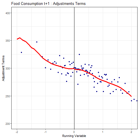
Figure 7.1: Adjustment terms in the empirical application.

Notes: The figure presents the adjustment terms (for one split of the data) obtained using SuperLearner for the food consumption one year after the program was introduced. Each blue dot represents the mean of approximately 20 observations. The solid lines represents the local linear fit with triangular kernel and bandwidth $h=0.6$.

7.3.  Adjustment Terms

As explained above, our analysis assumes that the conditional expectation functions of transformations of the covariates given the running variable vary smoothly around the cutoff. Most importantly, this must be satisfied for $\mathbb{E}(\bar{\eta}(Z_{i})|X_{i}=x)$, where $\bar{\eta}$ is the population function targeted by the estimated adjustment. To investigate the plausibility of this assumption, we can plot the estimated adjustment terms against the running variable and see whether there are any visually apparent discontinuities around the cutoff. Put differently, if we compute a “no covariates” RD estimator with $\widehat{\eta}_{s(i)}(Z_{i})$ as the outcome variable, we would expect to see an estimated jump with only small deviations from zero that are compatible with statistical noise if our assumptions hold. In Figure 7.1 shows such a plot for our empirical application. Each blue dot represents the mean of approximately 20 adjustment terms based on SuperLearner binned based on the running variable, and the red line shows the local linear regression fit with bandwidth $h=0.6$. We can see that the fit is very smooth, with essentially no jump at the cutoff, lending credibility to our assumptions.

8.  Conclusions

We have proposed a novel class of estimators that can make use of covariate information more efficiently than the linear adjustment estimators that are currently used widely in practice. In particular, our approach allows the use of modern machine learning tools to adjust for covariates, and is at the same time largely unaffected by the “curse of dimensionality”. Our estimator is also easy to implement in practice, and can be combined in a straightforward manner with existing methods for bandwidth choice and the construction of confidence intervals. For this reason, we expect it to be attractive for a wide range of economic applications.

Appendix A Proofs of the Main Results

In this section, we prove Theorems 4.1–4.3. To this end, we show a more general result that allows for a local polynomial regression of an arbitrary order $p$. We also use this result in Appendix B to establish the validity of the inference methods discussed in Section 5.1.

A.1.  Additional Notation

Denote the realizations of the running variable by $\mathbb{X}_{n}=(X_{i})_{i\in[n]}$. For $0\leq v\leq p$, we define feasible and infeasible estimators of the jump in the $v$-th derivative of the conditional expectation of the modified outcome at the cutoff using the $p$-th order local polynomial regression as:

$$\widehat{\tau}_{v,p}(h;\widehat{\eta}) =\sum_{i=1}^{n}w_{i,v,p}(h)M_{i}(\widehat{\eta}_{s(i)})\quad\text{and}\quad\widehat{\tau}_{v,p}(h;\bar{\eta})=\sum_{i=1}^{n}w_{i,v,p}(h)M_{i}(\bar{\eta}),$$

$$w_{i,v,p}(h) =w_{i,v,p}^{+}(h)-w_{i,v,p}^{-}(h),$$

$$w_{i,v,p}^{\star}(h) =e_{v}^{\top}\left(\sum_{i=1}^{n}K^{\star}_{h}(X_{i})\widetilde{X}_{p,i}\widetilde{X}_{p,i}^{\top}\right)^{-1}K^{\star}_{h}(X_{i})\widetilde{X}_{p,i}\quad\text{ for }\star\in\{+,-\},$$

with $\widetilde{X}_{p,i}=(1,X_{i},...,X_{i}^{p})^{\top}$, $K_{h}(v)=K(v/h)/h$, $K^{+}_{h}(v)=K_{h}(v)\mathbf{1}\{v\geq 0\}$, $K^{-}_{h}(v)=K_{h}(v)\mathbf{1}\{v<0\}$. Corresponding estimates of $\beta^{\star}_{v}(\bar{\eta})=\partial_{x}^{v}\mathbb{E}[M_{i}(\bar{\eta})|X_{i}=x]|_{x=0^{\star}}$ are:

$$\widehat{\beta}^{\star}_{v,p}(h;\widehat{\eta})=\sum_{i=1}^{n}w^{\star}_{i,v,p}(h)M_{i}(\widehat{\eta}_{s(i)})\quad\text{and}\quad\widehat{\beta}^{\star}_{v,p}(h;\bar{\eta})=\sum_{i=1}^{n}w^{\star}_{i,v,p}(h)M_{i}(\bar{\eta})\quad\text{for }\star\in\{+,-\}.$$

A.2.  General Result

In this subsection, we state and prove two theorems that generalize Theorems 4.1 and 4.2.

Theorem A.1.

Suppose that Assumptions 4.1–4.3 hold with $j\in\{1,...,p+1\}$ in Assumption 4.2. Then:

$$\widehat{\tau}_{0,p}(h;\widehat{\eta})=\widehat{\tau}_{0,p}(h;\bar{\eta})+O_{P}(t_{p}),$$

where $t_{p}=r_{n}(nh)^{-1/2}+\sum_{j=1}^{p}v_{j,n}h^{j}(nh)^{-1/2}+v_{p+1,n}h^{p+1}$.

In the proof of Theorem A.1, we will use the following lemma that collects some standard intermediate steps in the analysis of local polynomial estimators, taking into account cross-fitting.

Lemma A.1.

Suppose that Assumption 4.3 holds. For $s\in[S]$ and $\star\in\{-,+\}$, it holds that:

1. $\displaystyle\frac{S}{n}\sum_{i\in I_{s}}K_{h}^{\star}(X_{i})(X_{i}/h)^{j}=\mathbb{E}[K_{h}^{\star}(X_{i})(X_{i}/h)^{j}]+O_{p}((nh)^{-1/2})$ for $j\in\mathbb{N}$,

2. $\displaystyle\sum_{i\in I_{s}}w_{i,0,p}^{\star}(h)=1/S+O_{p}((nh)^{-1/2})$,

3. $\displaystyle\sum_{i\in I_{s}}w_{i,0,p}^{\star}(h)X_{i}^{j}=O_{p}(h^{j}(nh)^{-1/2})$ for $1\leq j\leq p$,

4. $\displaystyle\sum_{i\in I_{s}}|w_{i,0,p}^{\star}(h)X_{i}^{j}|=O_{P}(h^{j})$ for $j\in\mathbb{N}$,

5. $\displaystyle\sum_{i\in I_{s}}w_{i,0,p}^{\star}(h)^{2}=O_{P}((nh)^{-1})$.

Proof.

The results follow from standard kernel calculations. ∎

Proof of Theorem A.1.

To begin with, note that

$$\widehat{\tau}_{0,p}(h;\bar{\eta})-\widehat{\tau}_{0,p}(h;\widehat{\eta})=\sum_{s=1}^{S}G_{s}(p),\quad G_{s}(p)\equiv\sum_{i\in I_{s}}w_{i,0,p}(h)(\widehat{\eta}_{s}(Z_{i})-\bar{\eta}(Z_{i})).$$

Since $S$ is a fixed number, it suffices to show that $G_{s}(p)=O_{p}(t_{p})$ for $s\in\{1,...,S\}$. We analyze the expectation and variance of $G_{s}(p)$ conditional on $\mathbb{X}_{n}$ and $(W_{j})_{j\in I^{c}_{s}}$. We begin with the expectation. It holds with probability approaching one that

$$\left|\mathbb{E}[G_{s}(p)|\mathbb{X}_{n},(W_{j})_{j\in I^{c}_{s}}]\right| =\Big{|}\sum_{i\in I_{s}}w_{i,0,p}(h)\mathbb{E}[\widehat{\eta}_{s}(Z_{i})-\bar{\eta}(Z_{i})|X_{i},(W_{j})_{j\in I^{c}_{s}}]\Big{|}$$

$$\leq\sup_{\eta\in\mathcal{T}_{n}}\Big{|}\sum_{i\in I_{s}}w_{i,0,p}(h)\mathbb{E}[\eta(Z_{i})-\bar{\eta}(Z_{i})|X_{i}]\Big{|}.$$

Let $m(x;\eta)=\mathbb{E}[\eta(Z_{i})-\bar{\eta}(Z_{i})|X_{i}=x]$. Taylor’s theorem yields

$$m(X_{i};\eta)=m(0;\eta)+\sum_{j=1}^{p}\frac{1}{j!}\partial^{j}_{x}m(0;\eta)X_{i}^{j}+\frac{1}{(p+1)!}\partial^{p+1}_{x}m(\widetilde{x}_{i,p};\eta)X_{i}^{p+1}$$

for some $\widetilde{x}_{i,p}$ between $0$ and $X_{i}$. We analyze the three terms associated with different terms of Taylor’s expansion separately. We make use of Lemma A.1 in each step.

First, using the Cauchy-Schwarz inequality, we obtain that

$$\sup_{\eta\in\mathcal{T}_{n}}\Big{|}m(0;\eta)\sum_{i\in I_{s}}w_{i,0,p}(h)\Big{|}=\sup_{\eta\in\mathcal{T}_{n}}|m(0;\eta)|O_{p}((nh)^{-1/2})=O_{p}(r_{n}(nh)^{-1/2}).$$

Second, for $j\in\{1,...,p\}$, we have that

$$\sup_{\eta\in\mathcal{T}_{n}}\Big{|}\partial^{j}_{x}m(0;\eta)\sum_{i\in I_{s}}w_{i,0,p}(h)X_{i}^{j}\Big{|}=\sup_{\eta\in\mathcal{T}_{n}}|\partial^{j}_{x}m(0;\eta)|h^{j}O_{p}((nh)^{-1/2})=O_{p}(h^{j}(nh)^{-1/2}v_{j,n}).$$

Third, we note that

$$\sup_{\eta\in\mathcal{T}_{n}}\Big{|}\sum_{i\in I_{s}}w_{i,0,p}(h)\partial^{p+1}_{x}m(\widetilde{x}_{i};\eta)X_{i}^{p+1}\Big{|}\leq\sum_{i\in I_{s}}|w_{i,0,p}(h)X_{i}^{p+1}|\sup_{\eta\in\mathcal{T}_{n}}|\partial^{p+1}_{x}m(\widetilde{x}_{i};\eta)|=O_{p}(h^{p+1}v_{p+1,n}).$$

Next, we consider the conditional variance. It holds with probability approaching one that

$$\mathbb{V}\left[G_{s}(p)|\mathbb{X}_{n},(W_{j})_{j\in I^{c}_{s}}\right] =\sum_{i\in I_{s}}w_{i,0,p}(h)^{2}\mathbb{V}\left[\bar{\eta}(Z_{i})-\widehat{\eta}_{s}(Z_{i})|\mathbb{X}_{n},(W_{j})_{j\in I^{c}_{s}}\right]$$

$$\leq\sup_{\eta\in\mathcal{T}_{n}}\sum_{i\in I_{s}}w_{i,0,p}(h)^{2}\mathbb{E}[(\bar{\eta}(Z_{i})-\eta(Z_{i}))^{2}|X_{i}]$$

$$\leq\sup_{\eta\in\mathcal{T}_{n}}\sup_{x\in\mathcal{X}_{h}}\mathbb{E}[(\bar{\eta}(Z_{i})-\eta(Z_{i}))^{2}|X_{i}=x]\sum_{i\in I_{s}}w_{i,0,p}(h)^{2}$$

$$=O_{p}(r_{n}^{\;2}(nh)^{-1}),$$

where we use Lemma A.1 and Assumption 4.1 in the last step. The conditional convergence then implies the unconditional one (see Chernozhukov et al., 2018, Lemma 6.1). ∎

Theorem A.2.

Suppose that the assumptions of Theorem A.1 hold, Assumption 4.4 holds, and $\mathbb{E}[M_{i}(\bar{\eta})|X_{i}=x]$ is $p+1$ times continuously differentiable with $L$-Lipschitz continuous $p+1$ derivative bounded by $C$. Then

$$\sqrt{nh}\,V_{p}(\bar{\eta})^{-1/2}\left(\widehat{\tau}_{0,p}(h;\widehat{\eta})-\tau-h^{p+1}B_{p}\right)\overset{d}{\to}\mathcal{N}(0,1),$$

where, for some kernel constants $\bar{\nu}_{p}$ and $\bar{\kappa}_{p}$,

$$B_{p,n} =\frac{\bar{\nu}_{p}}{2}\left(\partial_{x}^{p+1}\mathbb{E}[M_{i}(\bar{\eta})|X_{i}=x]\big{|}_{x=0^{+}}+(-1)^{p}\partial_{x}^{p+1}\mathbb{E}[M_{i}(\bar{\eta})|X_{i}=x]\big{|}_{x=0^{-}}\right)+o_{P}(1),$$

$$V_{p}(\bar{\eta}) =\frac{\bar{\kappa}_{p}}{f_{X}(0)}\left(\mathbb{V}[M_{i}(\bar{\eta})|X_{i}=0^{+}]+\mathbb{V}[M_{i}(\bar{\eta})|X_{i}=0^{-}]\right).$$

Proof of Theorem A.2.

By the conditional version of Lyapunov’s CLT, we obtain that

$$\text{se}_{0,p}(h;\bar{\eta})^{-1}\left(\widehat{\tau}_{0,p}(h;\bar{\eta})-\mathbb{E}[\widehat{\tau}_{0,p}(h;\bar{\eta})|\mathbb{X}_{n}]\right)\to\mathcal{N}(0,1).$$

where $\text{se}_{0,p}^{2}(h;\bar{\eta})=\sum_{i=1}^{n}w_{i,0,p}(h)^{2}\mathbb{V}[M_{i}(\bar{\eta})|X_{i}]$. By $L$-Lipschitz continuity of $\mathbb{V}[M_{i}(\bar{\eta})|X_{i}=x]$ in $x$, we obtain that

$$\text{se}_{0,p}^{2} (h;\bar{\eta})=\sum_{i=1}^{n}w_{i,0,p}^{-}(h)^{2}\mathbb{V}[M_{i}(\bar{\eta})|X_{i}=0^{-}]+\sum_{i=1}^{n}w_{i,0,p}^{+}(h)^{2}\mathbb{V}[M_{i}(\bar{\eta})|X_{i}=0^{+}]+o_{p}((nh)^{-1}).$$

It then follows from standard kernel calculations that $nh\,\text{se}_{0,p}^{2}(h;\bar{\eta})-V_{p}(\bar{\eta})=o_{P}(1)$ and $\mathbb{E}[\widehat{\tau}_{0,p}(h;\bar{\eta})|\mathbb{X}_{n}]-\tau=B_{p}h^{p+1}+o_{p}(h^{p+1})$ for some constant $B_{p}$. ∎

A.3.  Proofs of Theorems 4.1–4.3

Theorems 4.1 and 4.2 follow directly from the general results in Theorems A.1 and A.2 with $p=1$. It remains to prove Theorem 4.3. For any $\eta\in\mathcal{V}$, it holds that

$$\frac{2f_{X}(0)}{\bar{\kappa}}V(\eta)=\mathbb{V}[Y_{i}-\mu_{0}^{+}(Z_{i})|X_{i}=0^{+}]+\mathbb{V}[Y_{i}-\mu_{0}^{-}(Z_{i})|X_{i}=0^{-}]+R(\eta),$$

where the first two terms on the right-hand side do not depend on $\eta$, and

$$R(\eta)=\mathbb{V}[\mu_{0}^{+}(Z_{i})-\eta(Z_{i})|X_{i}=0^{+}]+\mathbb{V}[\mu_{0}^{-}(Z_{i})-\eta(Z_{i})|X_{i}=0^{-}].$$

Further, it holds that

$$R(\eta)=R(\eta_{0}+\eta-\eta_{0}) =\mathbb{V}\left[\frac{1}{2}(\mu_{0}^{+}(Z_{i})-\mu_{0}^{-}(Z_{i}))-(\eta(Z_{i})-\eta_{0}(Z_{i}))|X_{i}=0^{+}\right]$$

$$\quad+\mathbb{V}\left[-\frac{1}{2}(\mu_{0}^{+}(Z_{i})-\mu_{0}^{-}(Z_{i}))-(\eta(Z_{i})-\eta_{0}(Z_{i}))|X_{i}=0^{-}\right]$$

$$=R(\eta_{0})+2\mathbb{V}[\eta(Z_{i})-\eta_{0}(Z_{i})|X_{i}=0],$$

where in the last step we use the assumption on continuity of conditional covariances. The theorem follows from the above decomposition by taking the difference $V(\eta^{(a)})-V(\eta^{(b)})$ for arbitrary $\eta^{(a)}$ and $\eta^{(b)}$ in $\mathcal{V}$.∎

Appendix B Details on Section 5.1: Inference

In this section, we formally show that, under suitable assumptions, existing procedures for bandwidth selection and construction of confidence intervals based on “no covariates” estimators can be directly applied to the modified data $\{(X_{i},M_{i}(\widehat{\eta}))\}_{i\in[n]}$.

B.1.  Standard Errors

We propose a consistent standard error for $\widehat{\tau}_{v,p}(h;\widehat{\eta})$ of the form

$$\widehat{se}^{2}_{v,p}(h;\widehat{\eta})=\sum_{i=1}^{n}w_{i,v,p}^{2}(h)\widehat{\sigma}_{i}^{2}(\widehat{\eta}),$$

where $\widehat{\sigma}_{i}^{2}(\widehat{\eta})$ is a nearest-neighbor estimator of the variance ${\sigma_{i}^{2}(\bar{\eta})=\mathbb{V}[M_{i}(\bar{\eta})|X_{i}]}$:

$$\widehat{\sigma}^{2}_{i}(\widehat{\eta}) =\left(M_{i}(\widehat{\eta}_{s(i)})-\frac{1}{R}\sum_{j\in\mathcal{R}_{i}}M_{j}(\widehat{\eta}_{s(j)})\right)^{2},$$

with $\mathcal{R}_{i}$ is the set of $R$ nearest neighbors of unit $i$ in terms of their running variable realization on the respective side of the cutoff. Establishing consistency of this standard error requires the following technical assumption on the first stage estimator, which is implied by our main assumptions, for example, if $M_{i}(\bar{\eta})$ is bounded.

Assumption B.1.

For all $s\in[S]$, it holds that $\sum_{i\in[n]}w_{i,v,p}^{2}(h)\iota_{i}(\widehat{\eta})=o_{P}((nh^{1+2v})^{-1})$ for $0\leq v\leq p$, where

$$\iota_{i}(\widehat{\eta})=\sum_{\begin{subarray}{c}(j,l)\in\mathcal{R}_{i}^{2}\\ (j,l)\notin I^{2}_{s(i)}\end{subarray}}\left((\widehat{\eta}_{s(i)}(Z_{i})-\bar{\eta}(Z_{i}))-(\widehat{\eta}_{s(j)}(Z_{j})-\bar{\eta}(Z_{j}))\right)(M_{i}(\bar{\eta})-M_{l}(\bar{\eta})).$$

Proposition B.1.

Suppose that Assumptions 4.1–4.4 and B.1 hold. Moreover, suppose that Assumption 4.1 also holds with $\mathcal{X}_{h}$ replaced by $\widetilde{\mathcal{X}}_{h}$ that is an open set s.t. $\mathcal{X}_{h}\subset\widetilde{\mathcal{X}}_{h}$, and $\sup_{\eta\in\mathcal{T}_{n}}\sup_{x\in\widetilde{\mathcal{X}}_{h}}\mathbb{E}[(M_{i}(\eta)-\mathbb{E}[M_{i}(\eta)|X_{i}])^{4}|X_{i}=x]$ is bounded by $B$ for all $n\in\mathbb{N}$. Let further $\mathbb{E}[(M_{i}(\bar{\eta})|X_{i}=x]$ and $\mathbb{V}[(M_{i}(\bar{\eta})|X_{i}=x]$ be L-Lipschitz continuous. Then for all $0\leq v\leq p$, it holds that

$$nh^{1+2v}\left(\widehat{\text{se}}_{v,p}^{2}(h;\widehat{\eta})-se^{2}_{v,p}(h;\bar{\eta})\right)=o_{P}(1),$$

where $se^{2}_{v,p}(h;\bar{\eta})=\sum_{i=1}^{n}w_{i,v,p}^{2}(h)\sigma_{i}^{2}(\bar{\eta})$.

We note that Assumption B.1 could be dropped if we were to study a slight variation of $\widehat{se}^{2}_{v,p}(h;\widehat{\eta})$ in which we take the $R$ nearest neighbors of unit $i$ in terms of running variable values among units in the same fold to compute $\widehat{\sigma}^{2}_{i}(\widehat{\eta})$. However, proceeding like this would mean that existing software packages that compute nearest neighbor standard errors would have to be adapted, and could not be applied directly to the modified data $\{(X_{i},M_{i}(\widehat{\eta}))\}_{i\in[n]}$.

B.2.  Confidence intervals

We discuss three of types of confidence intervals for the RD parameter $\tau$.

B.2.1.  Confidence intervals with undersmoothing

We first consider confidence intervals that are based on an undersmoothing bandwidth of order $o(n^{-1/5})$. This choice of bandwidth implies that the smoothing bias shrinks to zero at a faster rate than the standard deviation and can hence be ignored when constructing confidence intervals. Let

$$CI^{us}_{1-\alpha}=\big{[}\widehat{\tau}(h;\widehat{\eta})\pm z_{\alpha}\widehat{\text{se}}(h;\widehat{\eta})\big{]},$$

where $z_{\alpha}$ is the $1-\alpha/2$ quantile of the standard normal distribution. Proposition B.2 shows that $CI^{us}_{1-\alpha}$ is asymptotically valid.

Proposition B.2.

Suppose that the assumptions of Proposition B.1 hold for $p=1$. If $nh^{5}=o(1)$, then $\mathbb{P}\big{(}\tau\in CI^{us}_{1-\alpha}\big{)}\geq 1-\alpha+o_{p}(1).$

B.2.2.  Robust bias-corrected confidence intervals

We now adapt the robust bias corrections of Calonico et al. (2014) to our setting. To keep the exposition transparent, we focus on the important special case where the bandwidth used to obtain the bias correction is the same as the main bandwidth. In this case, the local linear estimator with a bias correction is numerically equal to the local quadratic estimator (with the same bandwidth), i.e. $\widehat{\tau}_{0,2}(h;\widehat{\eta})$. Let

$$CI^{rbc}_{1-\alpha}=\big{[}\widehat{\tau}_{0,2}(h;\widehat{\eta})\pm z_{\alpha}\widehat{\text{se}}_{0,2}(h;\widehat{\eta})\big{]}.$$

Proposition B.3 shows that $CI^{rbc}_{1-\alpha}$ is asymptotically valid.

Proposition B.3.

Suppose that the assumptions of Theorem A.2 and Proposition B.1 hold for $p=2$. If $nh^{7}=o(1)$, then $\mathbb{P}\big{(}\tau\in CI^{rbc}_{1-\alpha}\big{)}\geq 1-\alpha+o_{p}(1).$

B.2.3.  Bias-aware confidence intervals

We consider a simplified version of the bias-aware approach of Armstrong and Kolesár (2018) that accounts for the asymptotic bias in our setting. Suppose that the researcher is willing to assume that the the second derivative of the conditional expectation function of the outcome $Y_{i}$ is bounded by $B_{Y}$. Then it follows from the results of Armstrong and Kolesár (2020) and our Theorem 4.2 that the smoothing bias of our covariate-adjusted RD estimator is bounded in absolute value by $\bar{b}(h)+o_{P}(h^{2})$, where

$$\bar{b}(h)=-\frac{B_{Y}}{2}\sum_{i=1}^{n}w_{i}(h)X_{i}^{2}\operatorname{sign}(X_{i}).$$

We note that this bound is independent of the chosen adjustment function. The proposed confidence interval is given by

$$CI^{ba}_{1-\alpha}=\left[\widehat{\tau}(h;\widehat{\eta})\pm z_{\alpha}(\bar{b}(h)/\widehat{\text{se}}_{0,1}(h;\widehat{\eta}))\,\widehat{\text{se}}_{0,1}(h;\widehat{\eta})\right].$$

where $z_{\alpha}(r)$ is the $1-\alpha/2$ quantile of the absolute value of the normal distribution with mean $r$ and variance one. Proposition B.4 shows that $CI^{ba}_{1-\alpha}$ is asymptotically valid.

Proposition B.4.

Suppose that the assumptions of Proposition B.1 hold for $p=1$. If $nh^{5}=O(1)$, then $\mathbb{P}\big{(}\tau\in CI^{ba}_{1-\alpha}\big{)}\geq 1-\alpha+o_{p}(1).$

In contrast to the results of Armstrong and Kolesár (2018, 2020), we only show that this confidence interval is valid for a fixed sequence of DGPs, rather than uniformly over a larger set of DGPs. We leave providing inference that is uniformly valid over how the covariates affect the outcome variable for future research.

B.3.  Consistent estimation of the MSE-optimal bandwidth

From Theorem 4.2, it follows that the bandwidth that minimizes the Asymptotic Mean Squared Error (AMSE) is given by

$$h_{AMSE}=\left(\frac{V(\bar{\eta})}{4B_{\textnormal{base}}^{2}}\right)^{1/5}n^{-1/5}.$$

This optimal bandwidth can be consistently estimated by applying the procedure of Calonico et al. (2014, s.6) to the modified data $\{(X_{i},M_{i}(\widehat{\eta}_{s(i)}))\}_{i\in[n]}$ using the following three steps.

Step 0. Initial bandwidths.

• Take any sequence $v_{n}$ such that $v_{n}\to 0$ and $nv_{n}\to\infty$. In practice, set $\widehat{v}_{n}=2.58\min\{S_{X},IQR/1.349\}n^{-1/5},$ where $S_{X}^{2}$ and $IQR_{X}$ denote, respectively, the sample variance and interquantile range of $\{X_{i}:1\leq i\leq n\}$.

• Choose $c_{n}$ s.t. $c_{n}\to 0$ and $nc_{n}^{7}\to\infty$. Specifically, let

  $$\widehat{c}_{n} =\widehat{C}_{n}^{1/9}n^{-1/9},$$

  $$\widehat{C}_{n} =\frac{7nv_{n}^{7}\widehat{se}_{3,3}(v_{n};\widehat{\eta})}{2\mathcal{B}_{3,3}^{2}\left(\widehat{\gamma}^{+}_{4,4}(\widehat{\eta})-\widehat{\gamma}^{-}_{4,4}(\widehat{\eta})\right)^{2}},$$

  where $\widehat{\gamma}^{\star}_{4,4}(\widehat{\eta})$ is the coefficient on $(1/4!)X_{i}^{4}$ in the fourth-order global polynomial regression using the modified data $\{(X_{i},M_{i}(\widehat{\eta}_{s(i)}))\}_{i\in[n]}$ on the respective side of the cutoff and $\mathcal{B}_{v,p}=\mathcal{B}^{+}_{v,p}-\mathcal{B}^{-}_{v,p}$, where $\mathcal{B}^{\star}_{v,p}$ for $\star\in\{+,-\}$ is the kernel constant in the leading bias term of $\widehat{\beta}^{\star}_{v,p}(h;\widehat{\eta})$.

Step 1. Choose a pilot bandwidth $b_{n}$ such that $b_{n}\to 0$ and $nb_{n}^{5}\to\infty$. In practice, estimate the AMSE-optimal bandwidth for the second derivative in the local quadratic regression:

$$\widehat{b}_{n} =\widehat{B}_{n}^{1/7}n^{-1/7},$$

$$\widehat{B}_{n} =\frac{5nv_{n}^{5}\widehat{se}_{2,2}(v_{n};\widehat{\eta})}{2\mathcal{B}^{2}_{2,2}\Big{(}\left(\widehat{\beta}^{+}_{3,3}(c_{n},\widehat{\eta})+\widehat{\beta}^{-}_{3,3}(c_{n};\widehat{\eta})\right)^{2}+3\widehat{se}_{3,3}(c_{n};\widehat{\eta})\Big{)}}.$$

Step 2. The main bandwidth $h_{AMSE}$ is estimated as

$$\widehat{h}_{n} =\widehat{H}_{n}^{1/5}n^{-1/5},$$

$$\widehat{H}_{n} =\frac{nv_{n}\widehat{se}_{0,1}(v_{n};\widehat{\eta})}{4\mathcal{B}^{2}_{0,1}\Big{(}\left(\widehat{\beta}^{+}_{2,2}(b_{n};\widehat{\eta})-\widehat{\beta}^{-}_{2,2}(b_{n};\widehat{\eta})\right)^{2}+3\widehat{se}_{2,2}(b_{n};\widehat{\eta})\Big{)}}.$$

Proposition B.5.

Suppose that the assumptions of Theorem A.2 and Proposition B.1 hold for $p=3$, $\mathcal{X}$ is bounded, $\mathbb{P}\big{[}1/C\leq|\widehat{\gamma}^{+}_{4,4}(\bar{\eta})-\widehat{\gamma}^{-}_{4,4}(\bar{\eta})|\leq C]\to 1$ for some $C>0$, and Assumption 4.1 holds with $\mathcal{X}_{h}$ replaced by $\mathcal{X}$. Suppose that $\beta^{+}_{v}(\bar{\eta})-(-1)^{v+1}\beta^{-}_{v}(\bar{\eta})$ is bounded and bounded away from zero for $v\in\{2,3\}$. Then $\widehat{c}_{n}\overset{p}{\to}0,\,n\widehat{c}_{n}^{\,7}\overset{p}{\to}\infty,\,\widehat{b}_{n}\overset{p}{\to}0,\,n\widehat{b}_{n}^{\,5}\overset{p}{\to}\infty$, and $\widehat{h}_{n}/h_{AMSE}\overset{p}{\to}1.$

B.4.  Proofs of Propositions B.1–B.5

B.4.1.  Proof of Proposition B.1

To begin with, we note that the weights $w_{i,v,p}(h)$ satisfy: (i) $\sum_{i\in[n]}w_{i,v,p}(h)^{2}=O_{P}((nh^{1+2v})^{-1})$and (ii) $\max_{i\in[n]}w_{i,v,p}(h)^{2}=o_{P}((nh^{1+2v})^{-1})$. This can be shown using standard kernel calculations.

The proof of Proposition B.1 consists in showing that $\widehat{\text{se}}_{v,p}^{2}(h;\widehat{\eta})$ is asymptotically equivalent to its infeasible version that uses the deterministic function $\bar{\eta}$, given by

$$\widehat{\text{se}}_{v,p}^{2}(h;\bar{\eta})=\sum_{i\in[n]}w_{i,v,p}^{2}(h)\bigg{(}M_{i}(\bar{\eta})-\frac{1}{R}\sum_{j\in\mathcal{R}_{i}}M_{j}(\bar{\eta})\bigg{)}^{2}.$$

Using arguments as in the proof of Theorem 4 in Noack and Rothe (2021), one can show that $\widehat{\text{se}}_{v,p}^{2}(h;\bar{\eta})-\text{se}_{v,p}^{2}(h;\bar{\eta})=o_{P}((nh^{1+2v})^{-1})$. It therefore remains to show that $\widehat{\text{se}}_{v,p}^{2}(h;\widehat{\eta})-\widehat{\text{se}}_{v,p}^{2}(h;\bar{\eta})=o_{P}((nh^{1+2v})^{-1})$. We express this difference as the sum of terms that are linear in $M_{i}(\widehat{\eta}_{s(i)})-M_{i}(\bar{\eta})=\bar{\eta}(Z_{i})-\widehat{\eta}_{s(i)}(Z_{i})$ and a quadratic remainder:

$$\widehat{\text{se}}_{v,p}^{2}(h;\widehat{\eta})-\widehat{\text{se}}_{v,p}^{2}(h;\bar{\eta})$$

$$\;=2\sum_{i\in[n]}w_{i,v,p}^{2}(h)\bigg{(}M_{i}(\bar{\eta})-\frac{1}{R}\sum_{j\in\mathcal{R}_{i}}M_{j}(\bar{\eta})\bigg{)}\bigg{(}M_{i}(\widehat{\eta}_{s(i)})-M_{i}(\bar{\eta})-\frac{1}{R}\sum_{j\in\mathcal{R}_{i}}(M_{j}(\widehat{\eta}_{s(j)})-M_{j}(\bar{\eta}))\bigg{)}$$

$$\;\quad+\sum_{i\in[n]}w_{i,v,p}^{2}(h)\bigg{(}M_{i}(\widehat{\eta}_{s(i)})-M_{i}(\bar{\eta})-\frac{1}{R}\sum_{j\in\mathcal{R}_{i}}(M_{j}(\widehat{\eta}_{s(j)})-M_{j}(\bar{\eta}))\bigg{)}^{2}$$

$$\;\equiv A_{1}+2A_{2}.$$

We first consider $A_{2}$. Let $C$ denote a generic constant that might change from line to line. It holds that

$$\frac{1}{C}A_{2} \leq\sum_{i=1}^{n}w_{i,v,p}^{2}(h)\bigg{(}(\widehat{\eta}_{s(i)}(Z_{i})-\bar{\eta}(Z_{i}))^{2}+\frac{1}{R}\sum_{j\in\mathcal{R}_{i}}(\widehat{\eta}_{s(j)}(Z_{j})-\bar{\eta}(Z_{j}))^{2}\bigg{)}$$

$$\leq\sum_{i=1}^{n}\bigg{(}w_{i,v,p}^{2}(h)+\frac{C}{R}\sum_{j:\;i\in R_{j}}w_{j,v,p}^{2}(h)\bigg{)}(\widehat{\eta}_{s(i)}(Z_{i})-\bar{\eta}(Z_{i}))^{2}$$

$$=\sum_{s\in[S]}\sum_{i\in I_{s}}\bigg{(}w_{i,v,p}^{2}(h)+\frac{C}{R}\sum_{j:\;i\in R_{j}}w_{j,v,p}^{2}(h)\bigg{)}(\widehat{\eta}_{s(i)}(Z_{i})-\bar{\eta}(Z_{i}))^{2}$$

$$\equiv\sum_{s\in[S]}A_{2,s}.$$

For all $s\in[S]$, it holds with probability approaching one that

$$\mathbb{E}[ A_{2,s}|\mathbb{X}_{n},\{W_{i}\}_{i\in I_{s}^{c}}]$$

$$\leq\sum_{i\in I_{s}}\left(w_{i,v,p}^{2}(h)+\frac{C}{R}\sum_{j:\;i\in R_{j}}w_{j,v,p}^{2}(h)\right)\sup_{\eta\in\mathcal{T}_{n}}\sup_{x\in\mathcal{X}_{h}}\mathbb{E}\left[(\eta(Z_{i})-\bar{\eta}(Z_{i}))^{2}|X_{i}=x\right]$$

$$\leq C\sum_{i=1}^{n}w_{i,v,p}^{2}(h)\sup_{\eta\in\mathcal{T}_{n}}\sup_{x\in\mathcal{X}_{h}}\mathbb{E}\left[(\eta(Z_{i})-\bar{\eta}(Z_{i}))^{2}|X_{i}=x\right]=O_{P}((nh^{1+2v})^{-1}r_{n}^{2}).$$

As $S$ is finite and $A_{2,s}$ is a positive random variable, it follows that $A_{2}=o_{P}((nh^{1+2v})^{-1})$.

To show that $A_{1}$ is of order $o_{P}((nh^{1+2v})^{-1})$, we separate the terms involving the nearest neighbors in the fold of unit $i$ and those that involve at least one neighbor from a different fold. Specifically, we have that:

$$A_{1} =\frac{1}{R^{2}}\sum_{i\in[n]}w_{i,v,p}^{2}(h)\bigg{(}\sum_{j,l\in\mathcal{R}_{i}}(M_{i}(\bar{\eta})-M_{l}(\bar{\eta}))\left((\widehat{\eta}_{s(i)}(Z_{i})-\bar{\eta}(Z_{i}))-(\widehat{\eta}_{s(j)}(Z_{j})-\bar{\eta}(Z_{j}))\right)\bigg{)}$$

$$=\frac{1}{R^{2}}\sum_{i\in[n]}w_{i,v,p}^{2}(h)\left(\sum_{\begin{subarray}{c}(j,l)\in\mathcal{R}_{i}^{2}\\ (j,l)\notin I^{2}_{s(i)}\end{subarray}}(M_{i}(\bar{\eta})-M_{l}(\bar{\eta}))\left((\widehat{\eta}_{s(i)}(Z_{i})-\bar{\eta}(Z_{i}))-(\widehat{\eta}_{s(j)}(Z_{j})-\bar{\eta}(Z_{j}))\right)\right)$$

$$\quad+\frac{1}{R^{2}}\sum_{s\in[S]}\sum_{i\in I_{s}}w_{i,v,p}^{2}(h)\bigg{(}\sum_{j,l\in\mathcal{R}_{i}\cap I_{s}}(M_{i}(\bar{\eta})-M_{l}(\bar{\eta}))\left((\widehat{\eta}_{s(i)}(Z_{i})-\bar{\eta}(Z_{i}))-(\widehat{\eta}_{s(j)}(Z_{j})-\bar{\eta}(Z_{j}))\right)\bigg{)}$$

$$\equiv A_{1,1}+\frac{1}{R^{2}}\sum_{s\in[S]}A_{1,2,s}.$$

By Assumption B.1, it holds that $A_{1,1}=o_{P}((nh^{1+2v})^{-1})$. For all $s\in[S]$, it holds with probability approaching one that

$$\mathbb{E}[ |A_{1,2,s}||\mathbb{X}_{n},\{W_{i}\}_{i\in I_{s}^{c}}]$$

$$\leq\sum_{i\in I_{s}}w_{i,v,p}^{2}(h)\sum_{j,l\in(\mathcal{R}_{i}\cap I_{s})\cup\{i\}}\mathbb{E}[|(M_{i}(\bar{\eta})-M_{l}(\bar{\eta}))(\widehat{\eta}_{s(j)}(Z_{j})-\bar{\eta}(Z_{j}))||\mathbb{X}_{n},\{W_{i}\}_{i\in I_{s}^{c}}]$$

$$\leq\sum_{i\in I_{s}}w_{i,v,p}^{2}(h)\sum_{j,l\in(\mathcal{R}_{i}\cap I_{s})\cup\{i\}}\sup_{\eta\in\mathcal{T}_{n}}\mathbb{E}[|(M_{i}(\bar{\eta})-M_{l}(\bar{\eta}))(\eta(Z_{j})-\bar{\eta}(Z_{j}))||\mathbb{X}_{n}]$$

$$\leq\sum_{i\in I_{s}}w_{i,v,p}^{2}(h)\sum_{j,l\in(\mathcal{R}_{i}\cap I_{s})\cup\{i\}}\left(\mathbb{E}[(M_{i}(\bar{\eta})-M_{l}(\bar{\eta}))^{2}|\mathbb{X}_{n}]\sup_{\eta\in\mathcal{T}_{n}}\mathbb{E}[(\eta(Z_{j})-\bar{\eta}(Z_{j}))^{2}|\mathbb{X}_{n}]\right)^{1/2}$$

$$=O_{P}((nh^{1+2v})^{-1}r_{n}),$$

where the last equality follows from Assumption 4.1 and the assumption of bounded second moments. Hence, $A_{1,2,s}=o_{p}((nh^{1+2v})^{-1})$, which concludes this proof. ∎

B.4.2.  Proof of Proposition B.2

Validity of the CI follows directly from asymptotic normality of the local linear estimator established in Theorem A.2 and the fact that the standard error is consistent. ∎

B.4.3.  Proof of Proposition B.3

Validity of the CI follows directly from asymptotic normality of the local quadratic estimator established in Theorem A.2 and the fact that the standard error is consistent. ∎

B.4.4.  Proof of Proposition B.4

Validity of the CI follows directly from asymptotic normality of the local linear estimator established in Theorem A.2, the fact that the standard error is consistent, and that the bias is bounded in absolute value by $\bar{b}(h)+o_{P}(h^{2})$. ∎

B.4.5.  Proof of Proposition B.5

The proposition follows, using the consistency of the standard error established in Proposition B.1, if the following claims hold:

1. $\widehat{\gamma}^{\star}_{4,4}(\widehat{\eta})-\widehat{\gamma}^{\star}_{4,4}(\bar{\eta})=o_{P}(1)$,

2. $\widehat{\beta}^{+}_{3,3}(c_{n};\widehat{\eta})+\widehat{\beta}^{-}_{3,3}(c_{n};\widehat{\eta})=\beta^{+}_{3}(\bar{\eta})+\beta^{-}_{3}(\bar{\eta})+o_{P}(1)$,

3. $\widehat{\beta}^{+}_{2,2}(b_{n};\widehat{\eta})-\widehat{\beta}^{-}_{2,2}(b_{n};\widehat{\eta})=\beta^{+}_{2}(\bar{\eta})-\beta^{-}_{2}(\bar{\eta})+o_{P}(1)$.

Part (i). First, note that

$$\widehat{\gamma}^{\star}_{4,4}(\widehat{\eta})-\widehat{\gamma}^{\star}_{4,4}(\bar{\eta})=e_{4}^{\prime}\left(\sum_{i=1}^{n}\widetilde{X}_{4,i}^{\star}{\widetilde{X}_{4,i}^{\star^{\top}}}\right)^{-1}\sum_{i=1}^{n}\widetilde{X}_{4,i}^{\star}(\bar{\eta}(Z_{i})-\widehat{\eta}_{s(i)}(Z_{i})),$$

where $\widetilde{X}^{+}_{4,i}=\widetilde{X}_{4,i}\mathbf{1}\{X_{i}\geq 0\}$ and $\widetilde{X}^{-}_{4,i}=\widetilde{X}_{4,i}\mathbf{1}\{X_{i}<0\}$. Further, for $s\in[S]$, we have that

$$\Big{|}\frac{S}{n}\sum_{i\in I_{s}}X_{i}^{j}(\bar{\eta}(Z_{i})-\widehat{\eta}_{s}(Z_{i}))\Big{|}\leq\sqrt{\frac{S}{n}\sum_{i\in I_{s}}X_{i}^{2j}}\sqrt{\frac{S}{n}\sum_{i\in I_{s}}(\bar{\eta}(Z_{i})-\widehat{\eta}_{s}(Z_{i}))^{2}}.$$

Note that, with probability approaching one,

$$\mathbb{E}\left[\frac{S}{n}\sum_{i\in I_{s}}(\bar{\eta}(Z_{i})-\widehat{\eta}_{s}(Z_{i}))^{2}\Big{|}\mathbb{X}_{n},(W_{j})_{j\in I_{s}^{c}}\right] \leq\sup_{\eta\in\mathcal{T}_{n}}\mathbb{E}\left[\frac{S}{n}\sum_{i\in I_{s}}(\bar{\eta}(Z_{i})-\eta(Z_{i}))^{2}\Big{|}\mathbb{X}_{n}\right]$$

$$\leq\sup_{\eta\in\mathcal{T}_{n}}\sup_{x\in\mathcal{X}}\mathbb{E}[(\bar{\eta}(Z_{i})-\eta(Z_{i}))^{2}|X_{i}=x]=o(1).$$

It follows that $\Big{|}\frac{S}{n}\sum_{i\in I_{s}}X_{i}^{j}(\bar{\eta}(Z_{i})-\widehat{\eta}_{s(i)}(Z_{i}))\Big{|}=o_{p}(1)$. Since $\mathcal{X}$ is bounded, the claim follows.

Part (ii) and (iii). Using steps as in the proof of Theorem A.1, for $p\in\{2,3\}$, we obtain that $\widehat{\beta}^{\star}_{p,p}(h;\widehat{\eta})-\widehat{\beta}^{\star}_{p,p}(h,\bar{\eta})=o_{P}(1)$. Moreover, under the assumptions made, $\widehat{\beta}^{\star}_{p,p}(h,\bar{\eta})-\beta^{\star}_{p}(\bar{\eta})=O_{P}(h+(nh^{1+2p})^{-1/2})$. The claims follow using the conditions on $b_{n}$ and $c_{n}$.∎

Appendix C Details on Section 5.3: Fuzzy RD Designs

We show asymptotic normality of the fuzzy covariate-adjusted RD estimator introduced in Section 5.3 and characterize the dependence of the asymptotic variance on the population analogues of the adjustment functions.

Proposition C.1.

Suppose that Assumptions 4.1–4.4 hold also with $T_{i}$ replacing $Y_{i}$, mutatis mutandis.

• It holds that

  $$\sqrt{nh}\,V_{\theta}(\bar{\eta}_{Y},\bar{\eta}_{T})^{-1/2}\left(\widehat{\theta}(h;\widehat{\eta}_{Y},\widehat{\eta}_{\scriptscriptstyle T})-\theta-B_{\theta}(\bar{\eta}_{Y},\bar{\eta}_{T})h^{2}\right)\to\mathcal{N}(0,1),$$

  where

  $$B_{\theta}(\bar{\eta}_{Y},\bar{\eta}_{T}) =\frac{\bar{\nu}}{2\tau_{T}}\left(\partial_{x}^{2}\mathbb{E}[Y_{i}-\theta T_{i}|X_{i}=x]\big{|}_{x=0^{+}}-\partial_{x}^{2}\mathbb{E}[Y_{i}-\theta T_{i}|X_{i}=x]\big{|}_{x=0^{-}}\right)+o_{P}(1),$$

  $$V_{\theta}(\bar{\eta}_{Y},\bar{\eta}_{T}) =\frac{\bar{\kappa}}{f_{X}(0)}\left(\mathbb{V}[U_{i}(\bar{\eta}_{Y},\bar{\eta}_{T})|X_{i}=0^{+}]+\mathbb{V}[U_{i}(\bar{\eta}_{Y},\bar{\eta}_{T})|X_{i}=0^{-}]\right),$$

  and $U_{i}(\bar{\eta}_{Y},\bar{\eta}_{T})=\left(Y_{i}-\theta T_{i}-(\bar{\eta}_{Y}(Z_{i})-\theta\bar{\eta}_{T}(Z_{i}))\right)/\tau_{T}$.

• Suppose additionally that the assumptions of Theorem 4.3 hold, mutatis mutandis, also with $T_{i}$ replacing $Y_{i}$ and the definition of $\mathcal{V}$ adjusted accordingly. Then, for any $\eta_{Y}^{(a)},\eta_{Y}^{(b)},\eta_{T}^{(a)},\eta_{T}^{(b)}\in\mathcal{V}$, it holds that

  $$V_{\theta} (\eta_{Y}^{(a)},\eta_{T}^{(a)})-V_{\theta}(\eta_{Y}^{(b)},\eta_{T}^{(b)})$$

  $$=\frac{2\bar{\kappa}}{\tau_{T}^{2}f_{X}(0)}\left(\mathbb{V}[\eta_{Y,0}(Z_{i})-\theta\eta_{T,0}(Z_{i})-(\eta_{Y}^{(a)}(Z_{i})-\theta\eta_{T}^{(a)}(Z_{i}))|X_{i}=0]\right.$$

  $$\qquad\left.-\mathbb{V}[\eta_{Y,0}(Z_{i})-\theta\eta_{T,0}(Z_{i})-(\eta_{Y}^{(b)}(Z_{i})-\theta\eta_{T}^{(b)}(Z_{i}))|X_{i}=0]\right).$$

Proof.

We first note that

$$\widehat{\theta}(h;\widehat{\eta}_{Y},\widehat{\eta}_{T})-\widehat{\theta}(h;\bar{\eta}_{Y},\bar{\eta}_{T})=O_{P}((r_{n}(nh)^{-1/2}+v_{1,n}h(nh)^{-1/2}+v_{2,n}h^{2})^{2}).$$

This equality is an immediate consequence of Theorem 4.1 and an application of the continuous mapping theorem as $|\tau_{T}|>0$. Further, using a mean-value expansion, it follows that

$$\widehat{\theta}(h;\bar{\eta}_{Y},\bar{\eta}_{T})-\theta=\frac{1}{\tau_{T}}(\widehat{\tau}_{Y}(h;\bar{\eta}_{Y})-\tau_{Y})-\frac{\tau_{Y}}{\tau_{T}^{2}}(\widehat{\tau}_{T}(h;\bar{\eta}_{T})-\tau_{T})+\widehat{\rho}(\bar{\eta}_{T},\bar{\eta}_{Y})$$

with

$$\widehat{\rho}(\bar{\eta}_{T},\bar{\eta}_{Y})=\frac{\widehat{\tau}_{Y}(h;\bar{\eta}_{Y})(\widehat{\tau}_{T}(h;\bar{\eta}_{T})-\tau_{T})^{2}}{2\widehat{\tau}_{T}^{*}(h;\bar{\eta}_{T})^{3}}-\frac{(\widehat{\tau}_{Y}(h;\bar{\eta}_{Y})-\tau_{Y})(\widehat{\tau}_{T}(h;\bar{\eta}_{T})-\tau_{T})}{\tau_{T}^{2}},$$

where $\widehat{\tau}_{T}^{*}(h;\eta_{T})$ is some intermediate value between $\tau_{T}$ and $\widehat{\tau}_{T}(h;\bar{\eta}_{T})$. Given our assumptions, it follows that

$$\widehat{\rho}(\widehat{\eta}_{T},\widehat{\eta}_{Y})=O_{P}\big{(}((nh)^{-1/2}+h^{2})^{2}\big{)}.$$

Part (i) follows analogously to Theorems 4.1 and 4.2 and Part (ii) follows from Theorem 4.3. ∎

Appendix D Additional Simulation Results

In this section, we present further simulation results. Table LABEL:table:sim_baseline_all_estimators extends the results in Table LABEL:table::sim_baseline. We present results for the bias-aware approach discussed in the main text with a bandwidth that is chosen optimally for the standard RD estimator without covariates. By doing so, we focus on the effect that our covariate adjustments have on the constants in the bias and variance expressions of the asymptotic distribution while holding the bandwidth fixed. We can therefore see that the bias is the same across all methods, and we can still draw the same qualitative conclusions about the standard deviations of the covariate-adjusted RD estimators using different first-stage estimators as discussed in Section 6. We emphasize that the procedure of holding the bandwidth fixed is useful to understand the mechanics of our variance reduction procedure, but in practice we recommend choosing the bandwidth optimally for the given adjustment terms as it leads to narrower confidence intervals.

In Table LABEL:table:sim_baseline_all_estimators, we also consider bandwidth choice and confidence intervals constructions based on robust bias corrections and undersmoothing (the bandwidth for undersmoothing is chosen as $n^{-1/20}$ times the MSE-optimal bandwidth estimated using the rdrobust package). The linear adjustment estimators with cross-fitting are constructed analogously to the procedure described in Section 6.1. For flexible covariate adjustments, the bandwidth is chosen optimally for each adjustment function. The qualitative conclusions about the relative performance of different first-stage estimators in different models remain the same as discussed in the main text. The simulated average bandwidth of robust bias corrections is typically smaller than that of the bias-aware approach, and the confidence intervals are larger. This feature is known in the nonparametric literature.

In Figure LABEL:fig:ecdfs, we plot the empirical CDFs of the estimators considered in Section 6. These graphs illustrate the quality of the approximation obtained in Theorem 4.1. As predicted by our theory, for all DGPs, the entire distribution of the covariate-adjusted RD estimator using the ensemble combination of all feasible first-stage estimation methods is very similar to the one of the oracle estimator.

Appendix E Additional Empirical Estimation Results

In this section, we extend the empirical results from Section 7 by considering additional outcome variables and second-stage inference methods. Specifically, we consider four different outcome variables: food and non-food consumption, one year and two years after the program implementation. For the second stage, we employ bias-aware inference with different smoothness constants, robust bias corrections and a version of undersmoothing. As in Section 7, the results are based on 100 different data splits.

The magnitude of gains from using covariate adjustments varies across outcome variables, but the relative patterns remain the same in that our covariate adjustments based on the linear regression provide improvements upon the standard RD estimator, but SuperLearner adjustments generally perform better.

References

- Andrews (1994) Andrews, D. (1994): “Asymptotics for semiparametric econometric models via stochastic equicontinuity,” Econometrica, 62, 43–72.
- Armstrong and Kolesár (2018) Armstrong, T. B. and M. Kolesár (2018): “Optimal inference in a class of regression models,” Econometrica, 86, 655–683.
- Armstrong and Kolesár (2020) ——— (2020): “Simple and honest confidence intervals in nonparametric regression,” Quantitative Economics, 11, 1–39.
- Belloni et al. (2012) Belloni, A., D. Chen, V. Chernozhukov, and C. Hansen (2012): “Sparse models and methods for optimal instruments with an application to eminent domain,” Econometrica, 80, 2369–2429.
- Belloni et al. (2017) Belloni, A., V. Chernozhukov, I. Fernández-Val, and C. Hansen (2017): “Program Evaluation and Causal Inference With High-Dimensional Data,” Econometrica, 85, 233–298.
- Calonico et al. (2019) Calonico, S., M. D. Cattaneo, M. H. Farrell, and R. Titiunik (2019): “Regression Discontinuity Designs Using Covariates,” The Review of Economics and Statistics, 101, 442–451.
- Calonico et al. (2014) Calonico, S., M. D. Cattaneo, and R. Titiunik (2014): “Robust nonparametric confidence intervals for regression-discontinuity designs,” Econometrica, 82, 2295–2326.
- Cattaneo et al. (2019) Cattaneo, M. D., N. Idrobo, and R. Titiunik (2019): A practical introduction to regression discontinuity designs: Foundations, Cambridge University Press.
- Chernozhukov et al. (2018) Chernozhukov, V., D. Chetverikov, M. Demirer, E. Duflo, C. Hansen, W. Newey, and J. Robins (2018): “Double/debiased machine learning for treatment and structural parameters,” The Econometrics Journal, 21, C1–C68.
- Chernozhukov et al. (2019) Chernozhukov, V., W. Newey, J. Robins, and R. Singh (2019): “Double/de-biased machine learning of global and local parameters using regularized Riesz representers,” Working Paper.
- Colangelo and Lee (2022) Colangelo, K. and Y.-Y. Lee (2022): “Double debiased machine learning nonparametric inference with continuous treatments,” Working Paper.
- Dong (2017) Dong, Y. (2017): “Alternative Assumptions to Identify LATE in Fuzzy Regression Discontinuity Designs,” Working Paper.
- Fan and Gijbels (1996) Fan, J. and I. Gijbels (1996): Local polynomial modelling and its applications, Chapman & Hall/CRC.
- Fan et al. (2020) Fan, Q., Y.-C. Hsu, R. P. Lieli, and Y. Zhang (2020): “Estimation of Conditional Average Treatment Effects With High-Dimensional Data,” Journal of Business & Economic Statistics, 0, 1–15.
- Frölich and Huber (2019) Frölich, M. and M. Huber (2019): “Including Covariates in the Regression Discontinuity Design,” Journal of Business & Economic Statistics, 37, 736–748.
- Gerard et al. (2020) Gerard, F., M. Rokkanen, and C. Rothe (2020): “Bounds on treatment effects in regression discontinuity designs with a manipulated running variable,” Quantitative Economics, 11, 839–870.
- Hahn (1998) Hahn, J. (1998): “On the role of the propensity score in efficient semiparametric estimation of average treatment effects,” Econometrica, 66, 315–331.
- Hahn et al. (2001) Hahn, J., P. Todd, and W. Van der Klaauw (2001): “Identification and Estimation of Treatment Effects with a Regression-Discontinuity Design,” Econometrica, 69, 201–209.
- Imbens and Kalyanaraman (2012) Imbens, G. and K. Kalyanaraman (2012): “Optimal bandwidth choice for the regression discontinuity estimator,” Review of Economic Studies, 79, 933–959.
- Imbens and Lemieux (2008) Imbens, G. W. and T. Lemieux (2008): “Regression discontinuity designs: A guide to practice,” Journal of Econometrics, 142, 615–635.
- Kennedy (2020) Kennedy, E. H. (2020): “Optimal doubly robust estimation of heterogeneous causal effects,” arXiv preprint arXiv:2004.14497.
- Kennedy et al. (2017) Kennedy, E. H., Z. Ma, M. D. McHugh, and D. S. Small (2017): “Nonparametric methods for doubly robust estimation of continuous treatment effects,” Journal of the Royal Statistical Society. Series B, Statistical Methodology, 79, 1229.
- Kolesár and Rothe (2018) Kolesár, M. and C. Rothe (2018): “Inference in Regression Discontinuity Designs with a Discrete Running Variable,” American Economic Review, 108, 2277––2304.
- Kreiß and Rothe (2023) Kreiß, A. and C. Rothe (2023): “Inference in regression discontinuity designs with high-dimensional covariates,” Econometrics Journal.
- Lee and Lemieux (2010) Lee, D. S. and T. Lemieux (2010): “Regression discontinuity designs in economics,” Journal of Economic Literature, 48, 281–355.
- McCrary (2008) McCrary, J. (2008): “Manipulation of the running variable in the regression discontinuity design: A density test,” Journal of econometrics, 142, 698–714.
- Newey (1994) Newey, W. (1994): “The Asymptotic Variance of Semiparametric Estimators,” Econometrica, 62, 1349–1382.
- Noack and Rothe (2021) Noack, C. and C. Rothe (2021): “Bias-aware inference in fuzzy regression discontinuity designs,” arXiv preprint arXiv:1906.04631.
- Robins and Rotnitzky (2001) Robins, J. M. and A. Rotnitzky (2001): “Comment on “Inference for semiparametric models: some questions and an answer” by P. Bickel and J. Kwon,” Statistica Sinica, 11, 920–936.
- Su et al. (2019) Su, L., T. Ura, and Y. Zhang (2019): “Non-separable models with high-dimensional data,” Journal of Econometrics, 212, 646–677.
- Wager et al. (2016) Wager, S., W. Du, J. Taylor, and R. J. Tibshirani (2016): “High-dimensional regression adjustments in randomized experiments,” Proceedings of the National Academy of Sciences, 113, 12673–12678.