Influence of inter-sublattice coupling on the terahertz nutation spin dynamics in antiferromagnets

Abstract

Spin-nutation resonance has been well-explored in one-sublattice ferromagnets. Here, we investigate the spin nutation in two-sublattice antiferromagnets as well as, for comparison, ferrimagnets with inter- and intra-sublattice nutation coupling. In particular, we derive the susceptibility of the two-sublattice magnetic system in response to an applied external magnetic field. To this end, the antiferromagnetic and ferrimagnetic (sub-THz) precession and THz nutation resonance frequencies are calculated. Our results show that the precession resonance frequencies and effective damping decrease with intra-sublattice nutation coupling, while they increase with inter-sublattice nutation in an antiferromagnet. However, we find that the THz nutation resonance frequencies decrease with both the intra and inter-sublattice nutation couplings. For ferrimagnets, conversely, we calculate two nutation modes with distinct frequencies, unlike antiferromagnets. The exchange-like precession resonance frequency of ferrimagnets decreases with intra-sublattice nutation coupling and increases with inter-sublattice nutation coupling, like antiferromagnets, but the ferromagnetic-like precession frequency of ferrimagnets is practically invariant to the intra and inter-sublattice nutation couplings.

I Introduction

Efficient spin manipulation at ultrashort timescales holds promise for applications in future magnetic memory technology [1, 2, 3, 4, 5]. Introduced by Landau and Lifshitz, the time evolution of magnetization $\bm{M}(\bm{r},t)$, can be described by the phenomenological Landau-Lifshitz-Gilbert (LLG) equation of motion, which reads [6, 7, 8, 9]

$$\dot{\bm{M}} =-\gamma\left(\bm{M}\times\bm{H}\right)+\frac{\alpha}{M_{0}}\left(\bm{M}\times\dot{\bm{M}}\right),$$ (1)

with the gyromagnetic ratio $\gamma$, constant magnetization amplitude $M_{0}$, and Gilbert damping parameter $\alpha$. The LLG equation consists of the precession of spins around a field $\bm{H}$ and transverse damping that aligns the spins towards the field direction. While the spin precessional motion can be explained by Zeeman-like field-spin coupling, there are several fundamental and microscopic mechanisms leading to Gilbert damping [10, 11, 12, 13, 14, 15, 16, 17, 18, 19, 20, 21, 22].

When one approaches the femtosecond regime, however, the spin dynamics can not only be described by the traditional LLG dynamical equation of motion [23, 24], but it has to be supplemented by a fast dynamics term due to magnetic inertia [25, 26, 27]. Essentially, the inclusion of magnetic inertia leads to a spin nutation at ultrashort timescales and can be described by a torque due to a double time-derivative of the magnetization i.e., $\bm{M}\times\ddot{\bm{M}}$ [26, 28]. The inertial LLG (ILLG) equation of motion has the form

$$\dot{\bm{M}} =-\gamma\left(\bm{M}\times\bm{H}\right)+\frac{\alpha}{M_{0}}\left(\bm{M}\times\dot{\bm{M}}\right)+\frac{\eta}{M_{0}}\left(\bm{M}\times\ddot{\bm{M}}\right),$$ (2)

with the inertial relaxation time $\eta$. In general, the Gilbert damping $\alpha$ and the inertial relaxation time $\eta$ are tensors [29], however, for an isotropic system, these parameters can be considered as scalars. The emergence of spin nutation has been attributed to an extension of Kamberský breathing Fermi surface model [30, 31], namely, an $s-d$-like interaction spin model between local magnetization and itinerant electrons [32, 33]. Moreover, the ILLG equation has been derived from the fundamental Dirac equation [29, 20]. Note that the Gilbert damping and inertial relaxation time are related to each other as the Gilbert damping is associated with the imaginary part of the susceptibility, while the inertial dynamics are associated with the real part of the susceptibility [20, 34]. The characteristic timescales of the nutation have been predicted to be in a range of $1-100$ fs [25, 32, 35, 36] and $1-10$ ps [36, 37]. More recently, it has been demonstrated that simple classical mechanical considerations superimposed with Gilbert dynamics naturally lead to magnetic inertial dynamics [38, 39].

Theoretically, the spin nutation has recently been extensively discussed for one-sublattice ferromagnets [25, 36, 40, 41, 42, 43, 44]. The nutation resonance has also been observed in experiments, however for two-sublattice ferromagnets [37]. A recent theoretical investigation predicts that the precession and nutation resonance frequencies may overlap in two-sublattice ferromagnets [45]. The spin nutation resonance has been observed at a higher frequency than ferromagnetic resonance, e.g., while the ferromagnetic resonance occurs in the GHz regime, the nutation resonance occurs in the THz regime [37, 46]. Moreover, the spin nutation shifts the ferromagnetic resonance frequency to a lower value. Although this shift is very small, the line-width of the resonance decreases, however, and thus the effective damping decreases, too.

Spin nutation effects have not yet comprehensively been discussed in two-antiparallel aligned sublattice magnetic systems (e.g., antiferromagnets, ferrimagnets). In a recent investigation, it has been predicted that the spin nutation in antiferromagnets may have much significance [46]. Due to sublattice exchange interaction, the antiferromagnetic resonance frequency lies in the THz regime, while the nutation resonance frequency has similar order of magnitude. This helps to detect the antiferromagnetic precession and nutation resonances experimentally as they fall in the same frequency range. Moreover, the calculated shift of the antiferromagnetic resonance frequency is stronger than that of a ferromagnet. Additionally, the nutation resonance peak is exchange enhanced [46], which is beneficial for detection in experiments. However, the previous investigation only considers the intra-sublattice inertial dynamics, while the effect of inter-sublattice inertial dynamics is unknown.

In a previous work, the LLG equation of motion with inter-sublattice Gilbert damping has been explored by Kamra et al. [47]. It was found that the introduction of inter-sublattice Gilbert damping enhances the damping [47, 48, 49]. In this study, we formulate the spin dynamical equations in a two-sublattice magnetic system with both intra and inter-sublattice inertial dynamics as well as inter and intra-sublattice Gilbert damping, extending thus previous work [46]. First, we derive the magnetic susceptibility with the inter-sublattice effects and compute the precession and nutation resonance frequencies. We find that the precession resonance frequency and the effective Gilbert damping decrease with the intra-sublattice nutation coupling in antiferromagnets, however, they increase with the inter-sublattice nutation. Unlike antiferromagnets, we find for ferrimagnets that the change of precession resonance frequencies is more pronounced with both intra and inter-sublattice nutation coupling constants in the exchange-like mode, but nearly negligible for the ferromagnetic mode.

The article is organized as follows. First, in Sec. II, we discuss the linear-response theory of spin dynamics to calculate the magnetic susceptibility with the intra and inter-sublattice nutation effects. In Sec. III, the precession resonance frequencies have been calculated with analytical and numerical tools for antiferromagnets (Sec. III.1) and ferrimagnets (Sec. III.2). We summarize the obtained results in Sec. IV.

II Linear-response susceptibility in two-sublattice magnets

For two-sublattice magnetic systems, namely $A$ and $B$ representing the two sublattices, the ILLG equations of motion read

$$\dot{\bm{M}}_{A} =-\gamma_{A}\left(\bm{M}_{A}\times\bm{H}_{A}\right)+\frac{\alpha_{AA}}{M_{A0}}\left(\bm{M}_{A}\times\dot{\bm{M}}_{A}\right)$$

$$+\frac{\alpha_{AB}}{M_{B0}}\left(\bm{M}_{A}\times\dot{\bm{M}}_{B}\right)+\frac{\eta_{AA}}{M_{A0}}\left(\bm{M}_{A}\times\ddot{\bm{M}}_{A}\right)$$

$$+\frac{\eta_{AB}}{M_{B0}}\left(\bm{M}_{A}\times\ddot{\bm{M}}_{B}\right),$$ (3)

$$\dot{\bm{M}}_{B} =-\gamma_{B}\left(\bm{M}_{B}\times\bm{H}_{B}\right)+\frac{\alpha_{BB}}{M_{B0}}\left(\bm{M}_{B}\times\dot{\bm{M}}_{B}\right)$$

$$+\frac{\alpha_{BA}}{M_{A0}}\left(\bm{M}_{B}\times\dot{\bm{M}}_{A}\right)+\frac{\eta_{BB}}{M_{B0}}\left(\bm{M}_{B}\times\ddot{\bm{M}}_{B}\right)$$

$$+\frac{\eta_{BA}}{M_{A0}}\left(\bm{M}_{B}\times\ddot{\bm{M}}_{A}\right).$$ (4)

In the above dynamical equations, the first terms relate to the spin precession, the second and third terms represent the intra and inter-sublattice Gilbert damping, and the last two terms classify the intra and inter-sublattice inertial dynamics. The intra-sublattice magnetization dynamics has been characterized with the Gilbert damping constants $\alpha_{AA}$, $\alpha_{BB}$ and inertial relaxation time $\eta_{AA}$ or $\eta_{BB}$, while the inter-sublattice dynamics is characterized by Gilbert damping $\alpha_{AB}$ or $\alpha_{BA}$ and inertial relaxation time $\eta_{AB}$ or $\eta_{BA}$. Note that the Gilbert damping parameters are dimensionless, however, inertial relaxation time has a dimension of time [26, 25, 29]. The extended equations of motions in Eqs. (II) and (4) represent general magnetization dynamics for two-sublattice magnets (e.g., antiferromagnets, ferrimagnets, two-sublattice ferromagnets, and so on).

The free energy of the considered two-sublattice system reads

$$\mathcal{F}\left(\bm{M}_{A},\bm{M}_{B}\right) =-H_{0}\left(M_{Az}+M_{Bz}\right)-\frac{K_{A}}{M^{2}_{A0}}M^{2}_{Az}$$

$$-\frac{K_{B}}{M^{2}_{B0}}M^{2}_{Bz}+\frac{J}{M_{A0}M_{B0}}\bm{M}_{A}\cdot\bm{M}_{B}\,.$$ (5)

Here, the first term defines the Zeeman coupling of two sublattice spins with an external field $\bm{H}_{0}=H_{0}\hat{\bm{z}}$. The second and third terms represent the anisotropy energies for the sublattice $A$ and $B$, respectively. The last term can be identified as the Heisenberg exchange energy between the two sublattices. Note that the Heisenberg coupling energy, $J>0$ for antiferromagnets and ferrimagnets, however $J<0$ for ferromagnetic-like coupling.

We calculate the effective field in the ILLG equation as the derivative of free energy in Eq. (5) with respect to the corresponding magnetization

$$\bm{H}_{A} =-\frac{\partial\mathcal{F}\left(\bm{M}_{A},\bm{M}_{B}\right)}{\partial\bm{M}_{A}}$$

$$=\left(H_{0}+\frac{2K_{A}}{M^{2}_{A0}}M_{Az}\right)\hat{\bm{z}}-\frac{J}{M_{A0}M_{B0}}\bm{M}_{B}\,,$$ (6)

$$\bm{H}_{B} =-\frac{\partial\mathcal{F}\left(\bm{M}_{A},\bm{M}_{B}\right)}{\partial\bm{M}_{B}}$$

$$=\left(H_{0}+\frac{2K_{B}}{M^{2}_{B0}}M_{Bz}\right)\hat{\bm{z}}-\frac{J}{M_{A0}M_{B0}}\bm{M}_{A}\,.$$ (7)

First, in the ground state, we consider that the $A$ sublattice magnetization is $\bm{M}_{A}=M_{A0}\hat{\bm{z}}$, while the $B$ sublattice magnetization is antiparallel $\bm{M}_{B}=-M_{B0}\hat{\bm{z}}$, such that we can describe the antiferromagnets ($M_{A0}=M_{B0}$) and ferrimagnets ($M_{A0}>M_{B0}$). We then expand the magnetization around the ground state in small deviations, $\bm{M}_{A}=M_{A0}\hat{\bm{z}}+\bm{m}_{A}(t)$ and $\bm{M}_{B}=-M_{B0}\hat{\bm{z}}+\bm{m}_{B}(t)$. The small deviations $\bm{m}_{A/B}$ are induced by the transverse external field $\bm{h}_{A/B}(t)$.

For convenience, we work in the circularly polarized basis, i.e., $m_{A/B\pm}=m_{A/Bx}\pm\textrm{i}m_{A/By},\,\,h_{A/B\pm}=h_{A/Bx}\pm\textrm{i}h_{A/By}$, and define $\Omega_{A}=\gamma_{A}/M_{A0}(J+2K_{A}+H_{0}M_{A0}),\,\,\Omega_{B}=\gamma_{B}/M_{B0}(J+2K_{B}-H_{0}M_{B0})$. With the time-dependent harmonic fields and magnetizations $h_{A/B\pm},\,\,m_{A/B\pm}\propto e^{\pm{\rm i}\omega t}$, we obtain the magnetic susceptibility tensor [46]

$$\begin{pmatrix}m_{A\pm}\\ m_{B\pm}\end{pmatrix} =\frac{1}{\Delta_{\pm}}\begin{pmatrix}\dfrac{1}{\gamma_{B}M_{B0}}\left(\Omega_{B}\pm{\rm i}\omega\alpha_{BB}-\omega^{2}\eta_{BB}+\omega\right)&-\dfrac{1}{\gamma_{B}M_{A0}}\left(\dfrac{\gamma_{B}}{M_{B0}}J\pm{\rm i}\omega\alpha_{BA}-\omega^{2}\eta_{BA}\right)\\ -\dfrac{1}{\gamma_{A}M_{B0}}\left(\dfrac{\gamma_{A}}{M_{A0}}J\pm{\rm i}\omega\alpha_{AB}-\omega^{2}\eta_{AB}\right)&\dfrac{1}{\gamma_{A}M_{A0}}\left(\Omega_{A}\pm{\rm i}\omega\alpha_{AA}-\omega^{2}\eta_{AA}-\omega\right)\end{pmatrix}\begin{pmatrix}h_{A\pm}\\ h_{B\pm}\end{pmatrix}$$

$$=\chi_{\pm}^{AB}\begin{pmatrix}h_{A\pm}\\ h_{B\pm}\end{pmatrix}\,,$$ (8)

with the definition of the determinant $\Delta_{\pm}=\left(\gamma_{A}\gamma_{B}M_{A0}M_{B0}\right)^{-1}\left(\Omega_{A}\pm{\rm i}\omega\alpha_{AA}-\omega^{2}\eta_{AA}-\omega\right)\left(\Omega_{B}\pm{\rm i}\omega\alpha_{BB}-\omega^{2}\eta_{BB}+\omega\right)-\left(\gamma_{A}\gamma_{B}M_{A0}M_{B0}\right)^{-1}\left(\frac{\gamma_{A}}{M_{A0}}J\pm{\rm i}\omega\alpha_{AB}-\omega^{2}\eta_{AB}\right)\left(\frac{\gamma_{B}}{M_{B0}}J\pm{\rm i}\omega\alpha_{BA}-\omega^{2}\eta_{BA}\right)$. As one expects, the inter-sublattice Gilbert damping and inertial dynamical contributions arise in the off-diagonal components of the susceptibility tensor, while the intra-sublattice contributions are in the diagonal component of the susceptibility [46]. Note that without inertial dynamics terms, the expression for the susceptibility is in accordance with the one derived by Kamra et al. [47].

To find the resonance frequencies, the determinant $\Delta_{\pm}$ must go to zero, thus one has to solve the following fourth-order equation in frequency

$$\mathcal{A}_{\pm}\omega^{4}+\mathcal{B}_{\pm}\omega^{3}+\mathcal{C}_{\pm}\omega^{2}+\mathcal{D}_{\pm}\omega+\mathcal{E}_{\pm}=0\,,$$ (9)

where the coefficients have the following forms

$$\mathcal{A}_{\pm} = \eta_{AA}\eta_{BB}-\eta_{AB}\eta_{BA},$$ (10)

$$\mathcal{B}_{\pm} = \mp{\rm i}\left(\alpha_{AA}\eta_{BB}+\alpha_{BB}\eta_{AA}\right)-\left(\eta_{AA}-\eta_{BB}\right)$$ (11)

$$\pm{\rm i}\left(\alpha_{AB}\eta_{BA}+\alpha_{BA}\eta_{AB}\right),$$

$$\mathcal{C}_{\pm} = -1\pm{\rm i}\left(\alpha_{AA}-\alpha_{BB}\right)-\left(\Omega_{A}\eta_{BB}+\Omega_{B}\eta_{AA}\right)$$ (12)

$$-\alpha_{AA}\alpha_{BB}+\left(\frac{\gamma_{A}}{M_{A0}}\eta_{BA}+\frac{\gamma_{B}}{M_{B0}}\eta_{AB}\right)J$$

$$+\alpha_{AB}\alpha_{BA},$$

$$\mathcal{D}_{\pm} = \left(\Omega_{A}-\Omega_{B}\right)\pm{\rm i}\left(\Omega_{A}\alpha_{BB}+\Omega_{B}\alpha_{AA}\right)$$ (13)

$$\mp{\rm i}\left(\frac{\gamma_{A}}{M_{A0}}\alpha_{BA}+\frac{\gamma_{B}}{M_{B0}}\alpha_{AB}\right)J,$$

$$\mathcal{E}_{\pm} = \Omega_{A}\Omega_{B}-\frac{\gamma_{A}\gamma_{B}}{M_{A0}M_{B0}}J^{2}\,.$$ (14)

The solutions of the above equation (9) result in four different frequencies in the presence of a finite external field. Two of those frequencies can be associated with the magnetization precession resonance, $\omega_{\rm p\pm}$ (positive and negative modes) that exists even without nutation. The other two frequencies dictate the nutation resonance frequencies, $\omega_{\rm n\pm}$ (positive and negative modes).

III Results and Discussion

The intrinsic intra-sublattice inertial dynamics have been discussed extensively in Ref. [46]. Essentially, the resonance frequencies and effective damping decrease with increasing intra-sublattice inertial relaxation time for antiferromagnets and ferrimagnets. Therefore, we consider a constant intra-sublattice inertial relaxation time in this work. In this section, we specifically discuss the effects of inter-sublattice nutation in both antiferromagnets and ferrimagnets.

III.1 Antiferromagnets

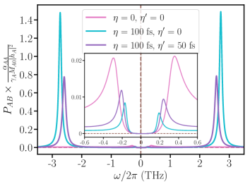
Figure 1: The calculated dissipated power vs. frequency for an antiferromagnet with $M_{A0}=M_{B0}=2\,\mu_{B}$, and various values of the intra- and inter-sublattice nutations parameters, $\eta$ and $\eta^{\prime}$. The inset shows the dissipated power close to the precession resonance frequencies. The other used parameters are $\gamma_{A}=\gamma_{B}=1.76\times 10^{11}$ T^-1s^-1, $J=10^{-21}$ J, $K_{A}=K_{B}=10^{-23}$ J, $H_{0}=1$ T, $\alpha_{AA}=\alpha_{BB}=0.05$, $\alpha_{AB}=\alpha_{BA}=0$, $\eta_{AA}=\eta_{BB}=\eta$ and $\eta_{AB}=\eta_{BA}=\eta^{\prime}$.

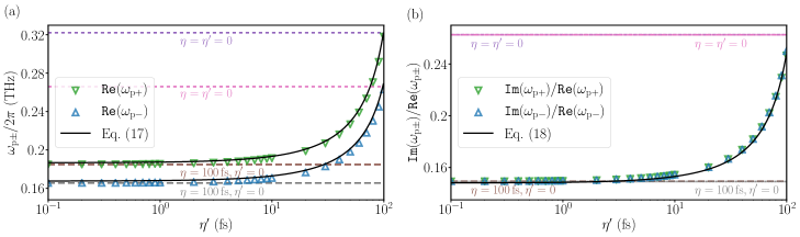
Figure 2: The calculated precession frequencies as a function of inter-sublattice nutation $\eta^{\prime}$ for an antiferromagnet, setting $M_{A0}=M_{B0}=2\,\mu_{B}$. The data points denote the numerical solution of Eq. (9) and the black lines correspond to the analytical solution in Eq. (16). (a) The real part of the resonance frequency, and (b) the ratio of imaginary and real part of the frequency have been plotted. The other used parameters are $\gamma_{A}=\gamma_{B}=1.76\times 10^{11}$ T^-1s^-1, $J=10^{-21}$ J, $K_{A}=K_{B}=K=10^{-23}$ J, $H_{0}=1$ T, $\alpha_{AA}=\alpha_{BB}=\alpha=0.05$, $\alpha_{AB}=\alpha_{BA}=0$, $\eta_{AA}=\eta_{BB}=\eta=100$ fs and $\eta_{AB}=\eta_{BA}=\eta^{\prime}$. The horizontal lines correspond to solutions with zero inter-sublattice nutation ($\eta^{\prime}=0$). Note that we show $\tt{Re}(\omega_{\textrm{p}-})$ as $-\tt{Re}(\omega_{{\rm p}-})$.

To start with, we calculate the frequency-dependent dissipated power of an antiferromagnet. Using the expressions for the susceptibility in Eq. (8), we calculate the dissipated power in the inertial dynamics with the following definition $P_{AB}=\dot{\bm{m}}_{A}\cdot\bm{h}_{A}+\dot{\bm{m}}_{B}\cdot\bm{h}_{B}=\frac{1}{2}\left(\dot{m}_{A+}h_{A-}+\dot{m}_{A-}h_{A+}+\dot{m}_{B+}h_{B-}+\dot{m}_{B-}h_{B+}\right)$ which leads to a complicated expression (not given). For convenience, we define $\alpha_{AA}=\alpha_{BB}=\alpha$, $\eta_{AA}=\eta_{BB}=\eta$. To focus on the inter-sublattice nutation $\eta_{AB}=\eta_{BA}=\eta^{\prime}$, we set the inter-sublattice Gilbert damping to zero, i.e., $\alpha_{AB}=\alpha_{BA}=0$, and choose $M_{A0}=M_{B0}=2\,\mu_{B}$. The exchange and anisotropy energies, magnetic moments used in the here-presented computations are comparable to a typical antiferromagnetic NiO [50, 51, 23] or CoO [52, 53] system. However, we mention that NiO or CoO bulk crystals have biaxial anisotropy. Also, the Gilbert damping of NiO is very small $\alpha\sim 10^{-4}$, i.e., less than the here-used value. In contrast, a large spin-orbit coupling in antiferromagnetic CrPt (that has $\sim$2 $\mu_{B}$ Cr moments) leads to a higher Gilbert damping $\alpha\sim 10^{-2}$ [54, 55]. Importantly, the inertial relaxation times $\eta$ and $\eta^{\prime}$ are not known in these antiferromagnetic systems. Our simulations pertain therefore to typical, selected model systems. We show the evaluated dissipated power with and without inertial dynamics for such antiferromagnet in Fig. 1. Note that the dissipated power has already been calculated in Ref. [46], however, without the inter-sublattice inertial dynamics. We can observe that while the intra-sublattice inertial dynamics decreases the precessional resonance frequencies (see the cyan lines in Fig. 1), the inter-sublattice inertial dynamics works oppositely. Note that the nutation resonance frequencies decrease with the introduction of inter-sublattice inertial dynamics.

To understand the effect of the inter-sublattice nutation terms, first, we solve the Eq. (9), considering again $\alpha_{AA}=\alpha_{BB}=\alpha$, $\eta_{AA}=\eta_{BB}=\eta$, $\eta_{AB}=\eta_{BA}=\eta^{\prime}$, and $\alpha_{AB}=\alpha_{BA}=0$. As the nutation in antiferromagnets is exchange enhanced [46], we calculate the effect of inter-sublattice terms on the precession and nutation frequencies, setting $\gamma_{A}=\gamma_{B}=\gamma$ and $M_{A0}=M_{B0}=M_{0}$ for antiferromagnets. Therefore, the fourth-order equation in Eq. (9) reduces to an equation with $\mathcal{A}_{\pm}^{\rm AFM}=\eta^{2}-\eta^{\prime 2}$, $\mathcal{B}_{\pm}^{\rm AFM}=\mp{\rm i}2\alpha\eta$, $\mathcal{C}_{\pm}^{\rm AFM}=-1-\left(\Omega_{A}+\Omega_{B}\right)\eta+2\frac{\gamma}{M_{0}}\eta^{\prime}J$, $\mathcal{D}_{\pm}^{\rm AFM}=\left(\Omega_{A}-\Omega_{B}\right)\pm{\rm i}\left(\Omega_{A}+\Omega_{B}\right)\alpha$, and $\mathcal{E}_{\pm}^{\rm AFM}=\Omega_{A}\Omega_{B}-\left(\frac{\gamma}{M_{0}}J\right)^{2}$. The solution of the above equation results in precession and nutation resonance frequencies for the two modes (positive and negative). Inserting the real and imaginary parts of the solutions $\omega_{\pm}={\tt Re}\left(\omega_{\pm}\right)+{\rm i}{\tt Im}(\omega_{\pm})$, we numerically calculate the precession resonance frequencies and effective damping (the ratio of imaginary and real frequencies) for an antiferromagnet as a function of inter-sublattice nutation. The results are shown in Fig. 2, where the data points correspond to the numerical solutions.

On the other hand, the fourth-order equation, $\mathcal{A}_{+}^{\rm AFM}\omega^{4}+\mathcal{B}_{+}^{\rm AFM}\omega^{3}+\mathcal{C}_{+}^{\rm AFM}\omega^{2}+\mathcal{D}_{+}^{\rm AFM}\omega+\mathcal{E}_{+}^{\rm AFM}=0$ can analytically be solved using the considerations that $K_{A}=K_{B}=K$, $J\gg K$, $M_{0}H_{0}$ and $\alpha\ll 1$. Therefore, one has $\Omega_{A}=\Omega_{B}\approx\gamma(J+2K)/M_{0}$. Essentially, the fourth-order equation reduces to

$$\left(\eta^{2}-\eta^{\prime 2}\right)\omega^{4}-\left[1+2\frac{\gamma\eta(J+2K)}{M_{0}}-2\frac{\gamma\eta^{\prime}J}{M_{0}}\right]\omega^{2}$$

$$-2{\rm i}\alpha\eta\omega_{(0)}^{3}+2\gamma H_{0}\omega_{(0)}+\frac{2{\rm i}\gamma\alpha}{M_{0}}\left(J+2K\right)\omega_{(0)}$$

$$+\frac{\gamma^{2}}{M_{0}^{2}}\left(J+2K\right)^{2}-\frac{\gamma^{2}J^{2}}{M_{0}^{2}}-\gamma^{2}H_{0}^{2}=0\,,$$ (15)

with $\omega_{(0)}$ being the solution of the above equation for $\alpha=0$ and $H_{0}=0$. The solutions of the above equation are rather simple and provide the two precession frequency modes (positive and negative) for antiferromagnets. Expanding the solutions of Eq. (15) up to the first order in $\alpha$ and $H_{0}$, and also in first order in $K/J\ll 1$, the precession resonance frequencies are obtained (neglecting the higher-order in $\omega_{(0)}$-terms) as

$$\omega_{\rm p\pm} \approx\pm\frac{\gamma}{M_{0}}\frac{\sqrt{4K\left(K+J\right)}}{\sqrt{1+\dfrac{4\gamma\eta K}{M_{0}}+\dfrac{2\gamma J}{M_{0}}\left(\eta-\eta^{\prime}\right)}}$$

$$+\frac{\gamma H_{0}+{\rm i}\dfrac{\gamma\alpha}{M_{0}}\left(J+2K\right)}{\sqrt{1+\dfrac{4\gamma\eta K}{M_{0}}+\dfrac{2\gamma J}{M_{0}}\left(\eta-\eta^{\prime}\right)}}\leavevmode\nobreak\ \frac{|\omega_{(0)}|}{\dfrac{\gamma}{M_{0}}\sqrt{4K(K+J)}}.$$ (16)

Now substituting the $|\omega_{(0)}|$ from the leading term in the frequency expression into the perturbative terms in Eq. (16), the approximate precession frequencies are obtained as

$$\omega_{\rm p\pm} \approx \pm\frac{\gamma}{M_{0}}\frac{\sqrt{4K\left(K+J\right)}}{\sqrt{1+\dfrac{4\gamma\eta K}{M_{0}}+\dfrac{2\gamma J}{M_{0}}\left(\eta-\eta^{\prime}\right)}}$$ (17)

$$+\frac{\gamma H_{0}+{\rm i}\dfrac{\gamma\alpha}{M_{0}}\left(J+2K\right)}{1+\dfrac{4\gamma\eta K}{M_{0}}+\dfrac{2\gamma J}{M_{0}}\left(\eta-\eta^{\prime}\right)}.$$

This equation has been plotted in Fig. 2 as black lines. Note that, for $\omega_{\rm p-}$ we show for convenience $-\tt{Re}(\omega_{\rm p-})$ in Fig.  2(a) and in the following. Due to the presence of $\eta-\eta^{\prime}$ in the denominator of the frequency expressions, the precession resonance frequency increases when inter-sublattice nutation is taken into account ($\eta^{\prime}<\eta$), which explains the increase in frequency in Fig. 2(a). At the limit $\eta\rightarrow\eta^{\prime}$, the nutation (intra and inter-sublattice) does not play a significant role as the precession resonance frequency is decreased by a factor $\sqrt{1+\frac{4\gamma\eta K}{M_{0}}}$ which is very small due to $K\ll J$. Note that the two resonance frequencies are approximately 0.332 THz and 0.276 THz with $\alpha=0$ and $\eta=\eta^{\prime}=0$, while these two frequencies are 0.322 THz and 0.266 THz with $\alpha=0.05$ and $\eta=\eta^{\prime}=0$. The latter has been shown in Fig. 2(a) as dashed lines. Therefore, the Gilbert damping has already the effect that it reduces the resonance frequencies.

The effective Gilbert damping can be calculated using the ratio between the imaginary and real parts of the frequencies, i.e., the line width. From Eq. (17) one arrives at

$$\frac{{\tt Im}\left(\omega_{\rm p\pm}\right)}{{\tt Re}\left(\omega_{\rm p\pm}\right)}\! \approx\alpha\frac{(J+2K)}{\sqrt{4K(K+J)}}\frac{1}{\sqrt{1+\dfrac{4\gamma\eta K}{M_{0}}+\dfrac{2\gamma J}{M_{0}}\left(\eta-\eta^{\prime}\right)}}\,.$$ (18)

Note that the two resonance modes have the same effective damping. For ferromagnets, the exchange energies do not contribute and thus the effective damping remains the same as $\alpha$, in the absence of magnetic inertial terms (see [45]). However, in antiferromagnets the effective damping is enhanced due to the exchange interaction by a factor $\frac{(J+2K)}{\sqrt{4K(K+J)}}$, even without any inertial terms. As investigated earlier [46], the effective damping decreases with the intra-sublattice relaxation time. However, similar to the increase in frequency, the effective damping also increases with the inter-sublattice inertial relaxation time, as seen in Fig. 2(b). The analytical solution in Eq. (18) agrees excellently with the numerical solutions. Close to the limit $\eta^{\prime}\rightarrow\eta$, the effective Gilbert damping in Eq. (18) one expects the effective damping to be increased by a factor $\left({1+\frac{4\gamma\eta K}{M_{0}}}\right)^{-1/2}$, as can be seen in Fig. 2(b).

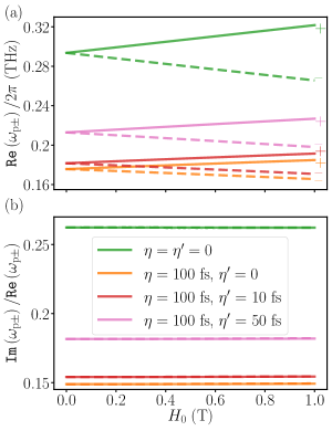
Figure 3: The calculated precession frequencies at several inter-sublattice relaxation times as a function of applied field for antiferromagnets using $M_{A0}=M_{B0}=2\,\mu_{B}$. The solid and dashed lines represent the positive and negative modes, respectively. (a) The real part of the resonance frequencies and (b) the ratio of imaginary and real part of the frequency have been plotted. The other used parameters are $\gamma_{A}=\gamma_{B}=1.76\times 10^{11}$ T^-1s^-1, $J=10^{-21}$ J, $K_{A}=K_{B}=K=10^{-23}$ J, $\alpha_{AA}=\alpha_{BB}=\alpha=0.05$, $\alpha_{AB}=\alpha_{BA}=0$, $\eta_{AA}=\eta_{BB}=\eta=100$ fs and $\eta_{AB}=\eta_{BA}=\eta^{\prime}$.

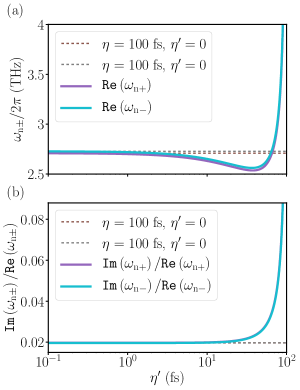
Figure 4: The calculated nutation frequencies as a function of inter-sublattice nutation for antiferromagnets using $M_{A0}=M_{B0}=2\,\mu_{B}$. (a) The real part of the nutation resonance frequencies and (b) the ratio of imaginary and real part of the nutation resonance frequency have been plotted. The other used parameters are $\gamma_{A}=\gamma_{B}=1.76\times 10^{11}$ T^-1s^-1, $J=10^{-21}$ J, $K_{A}=K_{B}=K=10^{-23}$ J, $H_{0}=1$ T, $\alpha_{AA}=\alpha_{BB}=\alpha=0.05$, $\alpha_{AB}=\alpha_{BA}=0$, $\eta_{AA}=\eta_{BB}=\eta=100$ fs and $\eta_{AB}=\eta_{BA}=\eta^{\prime}$.

Next, we discuss the field dependence of the resonance frequencies. The precession resonance frequencies and effective damping have been plotted as a function of the applied field $H_{0}$ for several inter-sublattice relaxation times in Fig. 3. As can be observed, at zero applied field, the two modes (positive and negative) coincide in antiferromagnets, a fact that can be seen from Eq. (17). However, the applied field induces the splitting of these two modes. The frequency splitting scales with $\left[1+\dfrac{4\gamma\eta K}{M_{0}}+\dfrac{2\gamma J}{M_{0}}\left(\eta-\eta^{\prime}\right)\right]^{-1}\!\gamma H_{0}$, meaning that the splitting is linear in the applied field, $H_{0}$. On the other hand, at a constant field, the splitting also depends on the inter- and intra-sublattice nutation. From Eq. (17), it is clear that the splitting is reduced with intra-sublattice nutation, while it is enhanced with inter-sublattice nutation. Such a conclusion can also be drawn from the numerical solutions in Fig. 3(a). The effective damping of the antiferromagnet remains field independent which can be observed in Fig. 3(b).

Proceeding as previously, we obtain the following nutation frequencies

$$\omega_{\rm n\pm} \approx\pm\frac{1}{\eta}\sqrt{\dfrac{1+\dfrac{4\gamma\eta K}{M_{0}}+\dfrac{2\gamma J}{M_{0}}\left(\eta-\eta^{\prime}\right)}{1-\dfrac{\eta^{\prime 2}}{\eta^{2}}}}\Bigg{(}1-$$

$$\dfrac{\dfrac{(\eta^{2}-\eta^{\prime 2})\gamma^{2}}{M_{0}}\times 4K(J+K)}{2\left[1+\dfrac{4\gamma\eta K}{M_{0}}+\dfrac{2\gamma J}{M_{0}}\left(\eta-\eta^{\prime}\right)\right]^{2}}\Bigg{)}$$

$$-\dfrac{\gamma H_{0}-{\rm i}\alpha\left[\dfrac{\eta}{\eta^{2}-\eta^{\prime 2}}+\dfrac{\gamma}{M_{0}}\left(J+2K\right)\right]}{1+\dfrac{4\gamma\eta K}{M_{0}}+\dfrac{2\gamma J}{M_{0}}\left(\eta-\eta^{\prime}\right)}\,.$$ (19)

Note that at the limit $\eta^{\prime}\rightarrow 0$, the nutation frequencies without the inter-sublattice coupling are recovered [46]. The dominant term in the calculated frequency is the first term in Eq. (19). With the introduction of inter-sublattice coupling $\eta^{\prime}$, both the numerator and denominator of the dominant frequency term decrease and therefore, the nutation frequencies approximately stay constant (with a slow decrease) with inter-sublattice nutation when $\eta>\eta^{\prime}$ as plotted in Fig. 4. However, in the limit $\eta^{\prime}\rightarrow\eta$, the denominator vanishes, and thus the nutation frequencies diverge as can be seen in Fig. 4. It is interesting to note that the inter-sublattice inertial dynamics increase the precession resonance frequencies, however, decrease the nutation frequency. Such observation is also consistent with the dissipated power in Fig. 1. The damping of the inertial dynamics also shows a similar behavior: it stays nearly constant with a divergence at the limit $\eta^{\prime}\rightarrow\eta$.

As mentioned before, the inertial relaxation times $\eta$ and $\eta^{\prime}$ are not known in for typical antiferromagnetic systems. Notwithstanding, we obtain the general result that the precession resonance frequencies decrease with intra-sublattice inertial dynamics, however, increase with inter-sublattice inertial dynamics. Thus, to experimentally realize the signature of inertial dynamics, an antiferromagnet with a higher ratio of intra to inter-sublattice inertial relaxation time ($\eta/\eta^{\prime}\gg 1$) is better suited.

III.2 Ferrimagnets

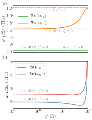
Figure 5: The calculated precession and nutation frequencies as a function of inter-sublattice nutation for ferrimagnets using $M_{A0}=5M_{B0}=10\,\mu_{B}$. The real part of the (a) precession resonance and (b) nutation resonance frequencies have been plotted. The other used parameters are $\gamma_{A}=\gamma_{B}=1.76\times 10^{11}$ T^-1s^-1, $J=10^{-21}$ J, $K_{A}=K_{B}=K=10^{-23}$ J, $H_{0}=1$ T, $\alpha_{AA}=\alpha_{BB}=\alpha=0.05$, $\alpha_{AB}=\alpha_{BA}=0$, $\eta_{AA}=\eta_{BB}=\eta=100$ fs and $\eta_{AB}=\eta_{BA}=\eta^{\prime}$.

Next, we consider a ferrimagnetic system where the magnetic moments in the two sublattices are different, i.e., $M_{A0}\neq M_{B0}$. In this case, the analytical solution of Eq. (9) becomes cumbersome. The main reason is that $\Omega_{A}\neq\Omega_{B}$ for ferrimagnets, in fact, we calculate $\Omega_{A}-\Omega_{B}=\frac{\gamma\left(J+2K\right)\left(M_{A0}-M_{B0}\right)}{M_{A0}M_{B0}}+2\gamma H_{0}$. For antiferromagnets, the magnetic moments in the two sublattices are exactly the same, i.e., $M_{A0}=M_{B0}$ and thus, within the approximation of $J\gg M_{0}H_{0}$, we find $\Omega_{A}=\Omega_{B}$ which simplifies the analytical solution of Eq. (9). Thus, we numerically solve the Eq. (9) to calculate the precession and nutation resonance frequencies for ferrimagnets. We consider the case where $M_{A0}=10\,\mu_{B}$ and $M_{B0}=2\,\mu_{B}$, reminiscent of rare-earth–transition-metal ferrimagnets as GdFeCo [2, 3] or TbCo [56, 57, 58]. However, we emphasize that the inertial relaxation times $\eta$ and $\eta^{\prime}$ are not known for these materials. The calculated precession frequencies are shown in Fig. 5(a). The effect of intra-sublattice inertial dynamics has already been studied in Ref. [46]. For ferrimagnets, the negative frequency mode appears to have a higher frequency (i.e., larger negative) than the positive one. However, both precession frequencies decrease with intra-sublattice relaxation time, $\eta$ [46]. We, therefore, have set the intra-sublattice relaxation time $\eta$ to 100 fs and vary the inter-sublattice relaxation time $\eta^{\prime}<\eta$. The upper precession resonance mode $\omega_{\rm p-}$ – the exchange-like mode – increases with the inter-sublattice relaxation time $\eta^{\prime}$, while the ferromagnetic-like mode $\omega_{\rm p+}$ shows a very small increase. Thus, for ferrimagnets, the change in precession frequencies is more significant in the exchange-like mode than in the ferromagnetic-like mode. At the limit $\eta^{\prime}\rightarrow\eta$, the precession resonance frequencies almost coincide with the resonance frequencies calculated at $\eta=\eta^{\prime}=0$, meaning that the inertial dynamics do not play any role for the precession resonance frequency. The latter can clearly be seen in Fig. 5(a). These observations are similar to the antiferromagnet as discussed earlier. The nutation resonance frequencies in Fig. 5(b) again decline with the inter-sublattice relaxation time showing a divergence at the limit $\eta^{\prime}\rightarrow\eta$. However, one can notice here two distinguishable nutation resonance frequencies unlike almost a single-valued nutation frequencies of antiferromagnets.

IV Summary

In summary, we have formulated a linear-response theory of the ILLG equations for antiferromagnets with inter- and intra-sublattice inertial dynamics. The calculation of the susceptibility tensor shows that the intra-sublattice terms appear in the diagonal elements, while the inter-sublattice terms appear in the off-diagonal elements. The dissipated power contains a precession resonance peak in the sub-THz regime for antiferromagnets, however, the introduction of inertial dynamics causes another peak, a nutation resonance peak at a higher, few THz frequency. Moreover, we observe that the inter-sublattice inertial dynamics work oppositely to the intra-sublattice inertial one. By finding the poles of the susceptibility, we calculate the precession and nutation resonance frequencies. While the precession resonance frequencies decrease with intra-sublattice relaxation time, the inter-sublattice inertial dynamics have the opposite effect. In fact, we observe that the magnetic inertia does not have any effect on the antiferromagnetic precession resonance at the limit $\eta^{\prime}\rightarrow\eta$. On the other hand, the THz nutation resonance frequency decreases slightly with the introduction of inter-sublattice inertial dynamics, however, showing a divergence at the limit $\eta^{\prime}\rightarrow\eta$. Our derived analytical theory explains such inter-sublattice contributions. Finally, for ferrimagnets, we find a similar behavior for the inter-sublattice inertial dynamics. However, the precession resonance frequency of the exchange-like mode depends significantly on the nutation couplings in contrast to that of the ferromagnetic-like mode that is practically independent of the nutation constants.

References

- Beaurepaire et al. [1996] E. Beaurepaire, J.-C. Merle, A. Daunois, and J.-Y. Bigot, Phys. Rev. Lett. 76, 4250 (1996).
- Stanciu et al. [2007] C. D. Stanciu, F. Hansteen, A. V. Kimel, A. Kirilyuk, A. Tsukamoto, A. Itoh, and Th. Rasing, Phys. Rev. Lett. 99, 047601 (2007).
- Vahaplar et al. [2009] K. Vahaplar, A. M. Kalashnikova, A. V. Kimel, D. Hinzke, U. Nowak, R. Chantrell, A. Tsukamoto, A. Itoh, A. Kirilyuk, and T. Rasing, Phys. Rev. Lett. 103, 117201 (2009).
- Carva et al. [2017] K. Carva, P. Baláž, and I. Radu, “Chapter 2 - laser-induced ultrafast magnetic phenomena,” in Handbook of Magnetic Materials, Vol. 26, edited by E. Brück (Elsevier, Amsterdam, 2017) pp. 291 – 463.
- John et al. [2017] R. John, M. Berritta, D. Hinzke, C. Müller, T. Santos, H. Ulrichs, P. Nieves, J. Walowski, R. Mondal, O. Chubykalo-Fesenko, J. McCord, P. M. Oppeneer, U. Nowak, and M. Münzenberg, Sci. Rep. 7, 4114 (2017).
- Landau and Lifshitz [1935] L. D. Landau and E. M. Lifshitz, Phys. Z. Sowjetunion 8, 153 (1935).
- Gilbert and Kelly [1955] T. L. Gilbert and J. M. Kelly, in American Institute of Electrical Engineers (New York, October 1955) pp. 253–263.
- [8] T. L. Gilbert, Ph.D. thesis, Illinois Institute of Technology, Chicago, 1956.
- Gilbert [2004] T. L. Gilbert, IEEE Trans. Magn. 40, 3443 (2004).
- Kamberský [1970] V. Kamberský, Can. J. Phys. 48, 2906 (1970).
- Kamberský [1976] V. Kamberský, Czech. J. Phys. B 26, 1366 (1976).
- Korenman and Prange [1972] V. Korenman and R. E. Prange, Phys. Rev. B 6, 2769 (1972).
- Kuneš and Kamberský [2002] J. Kuneš and V. Kamberský, Phys. Rev. B 65, 212411 (2002).
- Kamberský [2007] V. Kamberský, Phys. Rev. B 76, 134416 (2007).
- Tserkovnyak et al. [2002] Y. Tserkovnyak, A. Brataas, and G. E. W. Bauer, Phys. Rev. Lett. 88, 117601 (2002).
- Hickey and Moodera [2009] M. C. Hickey and J. S. Moodera, Phys. Rev. Lett. 102, 137601 (2009).
- Gilmore et al. [2007] K. Gilmore, Y. U. Idzerda, and M. D. Stiles, Phys. Rev. Lett. 99, 027204 (2007).
- Mondal et al. [2016] R. Mondal, M. Berritta, and P. M. Oppeneer, Phys. Rev. B 94, 144419 (2016).
- Mondal et al. [2018a] R. Mondal, M. Berritta, and P. M. Oppeneer, Phys. Rev. B 98, 214429 (2018a).
- Mondal et al. [2018b] R. Mondal, M. Berritta, and P. M. Oppeneer, J. Phys.: Condens. Matter 30, 265801 (2018b).
- Mondal et al. [2015a] R. Mondal, M. Berritta, K. Carva, and P. M. Oppeneer, Phys. Rev. B 91, 174415 (2015a).
- Mondal et al. [2015b] R. Mondal, M. Berritta, C. Paillard, S. Singh, B. Dkhil, P. M. Oppeneer, and L. Bellaiche, Phys. Rev. B 92, 100402(R) (2015b).
- Mondal et al. [2019] R. Mondal, A. Donges, U. Ritzmann, P. M. Oppeneer, and U. Nowak, Phys. Rev. B 100, 060409(R) (2019).
- Mondal et al. [2021a] R. Mondal, A. Donges, and U. Nowak, Phys. Rev. Research 3, 023116 (2021a).
- Ciornei et al. [2011] M.-C. Ciornei, J. M. Rubí, and J.-E. Wegrowe, Phys. Rev. B 83, 020410 (2011).
- [26] M.-C. Ciornei, Ph.D. thesis, Ecole Polytechnique, Universidad de Barcelona, 2010.
- Wegrowe and Ciornei [2012] J.-E. Wegrowe and M.-C. Ciornei, Am. J. Phys. 80, 607 (2012).
- Böttcher and Henk [2012] D. Böttcher and J. Henk, Phys. Rev. B 86, 020404 (2012).
- Mondal et al. [2017] R. Mondal, M. Berritta, A. K. Nandy, and P. M. Oppeneer, Phys. Rev. B 96, 024425 (2017).
- Fähnle and Illg [2011] M. Fähnle and C. Illg, J. Phys.: Condens. Matter 23, 493201 (2011).
- Fähnle et al. [2011] M. Fähnle, D. Steiauf, and C. Illg, Phys. Rev. B 84, 172403 (2011).
- Bhattacharjee et al. [2012] S. Bhattacharjee, L. Nordström, and J. Fransson, Phys. Rev. Lett. 108, 057204 (2012).
- Bajpai and Nikolić [2019] U. Bajpai and B. K. Nikolić, Phys. Rev. B 99, 134409 (2019).
- Thonig et al. [2017] D. Thonig, O. Eriksson, and M. Pereiro, Sci. Rep. 7, 931 (2017).
- Li et al. [2015] Y. Li, A.-L. Barra, S. Auffret, U. Ebels, and W. E. Bailey, Phys. Rev. B 92, 140413 (2015).
- Makhfudz et al. [2020] I. Makhfudz, E. Olive, and S. Nicolis, Appl. Phys. Lett. 117, 132403 (2020).
- Neeraj et al. [2020] K. Neeraj, N. Awari, S. Kovalev, D. Polley, N. Zhou Hagström, S. S. P. K. Arekapudi, A. Semisalova, K. Lenz, B. Green, J.-C. Deinert, I. Ilyakov, M. Chen, M. Bawatna, V. Scalera, M. d’Aquino, C. Serpico, O. Hellwig, J.-E. Wegrowe, M. Gensch, and S. Bonetti, Nat. Phys. 17, 245 (2020).
- Giordano and Déjardin [2020] S. Giordano and P.-M. Déjardin, Phys. Rev. B 102, 214406 (2020).
- Titov et al. [2021a] S. V. Titov, W. T. Coffey, Y. P. Kalmykov, M. Zarifakis, and A. S. Titov, Phys. Rev. B 103, 144433 (2021a).
- Cherkasskii et al. [2020] M. Cherkasskii, M. Farle, and A. Semisalova, Phys. Rev. B 102, 184432 (2020).
- Cherkasskii et al. [2021] M. Cherkasskii, M. Farle, and A. Semisalova, Phys. Rev. B 103, 174435 (2021).
- Lomonosov et al. [2021] A. M. Lomonosov, V. V. Temnov, and J.-E. Wegrowe, “Anatomy of inertial magnons in ferromagnets,” (2021), arXiv:2105.07376 [cond-mat.mes-hall] .
- Rahman and Bandyopadhyay [2021] R. Rahman and S. Bandyopadhyay, J. Phys.: Condens. Matter 33, 355801 (2021).
- Titov et al. [2021b] S. V. Titov, W. T. Coffey, Y. P. Kalmykov, and M. Zarifakis, Phys. Rev. B 103, 214444 (2021b).
- Mondal [2021] R. Mondal, J. Phys.: Condens. Matter 33, 275804 (2021).
- Mondal et al. [2021b] R. Mondal, S. Großenbach, L. Rózsa, and U. Nowak, Phys. Rev. B 103, 104404 (2021b).
- Kamra et al. [2018] A. Kamra, R. E. Troncoso, W. Belzig, and A. Brataas, Phys. Rev. B 98, 184402 (2018).
- Liu et al. [2017] Q. Liu, H. Y. Yuan, K. Xia, and Z. Yuan, Phys. Rev. Materials 1, 061401 (2017).
- Yuan et al. [2019] H. Y. Yuan, Q. Liu, K. Xia, Z. Yuan, and X. R. Wang, EPL 126, 67006 (2019).
- Hutchings and Samuelsen [1972] M. T. Hutchings and E. J. Samuelsen, Phys. Rev. B 6, 3447 (1972).
- Baierl et al. [2016] S. Baierl, J. H. Mentink, M. Hohenleutner, L. Braun, T.-M. Do, C. Lange, A. Sell, M. Fiebig, G. Woltersdorf, T. Kampfrath, and R. Huber, Phys. Rev. Lett. 117, 197201 (2016).
- Archer et al. [2008] T. Archer, R. Hanafin, and S. Sanvito, Phys. Rev. B 78, 014431 (2008).
- Archer et al. [2011] T. Archer, C. D. Pemmaraju, S. Sanvito, C. Franchini, J. He, A. Filippetti, P. Delugas, D. Puggioni, V. Fiorentini, R. Tiwari, and P. Majumdar, Phys. Rev. B 84, 115114 (2011).
- Besnus and Meyer [1973] M. J. Besnus and A. J. P. Meyer, phys. stat. sol. (b) 58, 533 (1973).
- Zhang et al. [2012] R. Zhang, R. Skomski, X. Li, Z. Li, P. Manchanda, A. Kashyap, R. D. Kirby, S.-H. Liou, and D. J. Sellmyer, J. Appl. Phys. 111, 07D720 (2012).
- Alebrand et al. [2012] S. Alebrand, M. Gottwald, M. Hehn, D. Steil, M. Cinchetti, D. Lacour, E. E. Fullerton, M. Aeschlimann, and S. Mangin, Appl. Phys. Lett. 101, 162408 (2012).
- Mangin et al. [2014] S. Mangin, M. Gottwald, C.-H. Lambert, D. Steil, V. Uhlíř, L. Pang, M. Hehn, S. Alebrand, M. Cinchetti, G. Malinowski, Y. Fainman, M. Aeschlimann, and E. E. Fullerton, Nat. Mater. 13, 286 (2014).
- Ciuciulkaite et al. [2020] A. Ciuciulkaite, K. Mishra, M. V. Moro, I.-A. Chioar, R. M. Rowan-Robinson, S. Parchenko, A. Kleibert, B. Lindgren, G. Andersson, C. S. Davies, A. Kimel, M. Berritta, P. M. Oppeneer, A. Kirilyuk, and V. Kapaklis, Phys. Rev. Mater. 4, 104418 (2020).