Three-dimensionality of the triadic resonance instability of a plane inertial wave

Abstract

We analyze theoretically and experimentally the triadic resonance instability (TRI) of a plane inertial wave in a rotating fluid. Building on the classical triadic interaction equations between helical modes, we show by numerical integration that the maximum growth rate of the TRI is found for secondary waves that do not propagate in the same vertical plane as the primary wave (the rotation axis is parallel to the vertical). In the inviscid limit, we prove this result analytically, in which case the change in the horizontal propagation direction induced by the TRI evolves from $60^{\circ}$ to $90^{\circ}$ depending on the frequency of the primary wave. Thanks to a wave generator with a large spatial extension in the horizontal direction of invariance of the forced wave, we are able to report experimental evidence that the TRI of a plane inertial wave is three-dimensional. The wavevectors of the secondary waves produced by the TRI are shown to match the theoretical predictions based on the maximum growth rate criterion. These results reveal that the triadic resonant interactions between inertial waves are very efficient at redistributing energy in the horizontal plane, normal to the rotation axis.

I Introduction

Rotating and stratified fluids allow the propagation of waves in their bulk, as a result of the restoring action of the Coriolis force and of the buoyancy force, respectively Greenspan1968 ; Lighthill1978 ; Sutherland2010 . Moreover, inertial waves in rotating fluids and internal gravity waves in stratified fluids share several remarkable features: they have similar dispersion relations linking the ratio between the wave frequency and the rotation rate or the buoyancy frequency to the tilt angle with the horizontal of the direction along which their energy propagates (with the rotation or gravity axis parallel to the vertical). As a consequence, their group and phase velocities are normal to each other. Also, their wavelength is independent of their frequency and is set by boundary conditions, viscous dissipation and non-linearities Brunet2019 . This leads to a variety of wave structures like self-similar beams Mowbray1967 ; Thomas1972 ; Flynn2003 ; Cortet2010 ; Machicoane2015 , plane waves Mercier2010 ; Bordes2012 ; Bourget2013 , resonant cavity modes Aldridge1969 ; McEwan1970 ; Maas2003b ; Boisson2012 ; Boisson2012b and even cavity limit cycles called wave attractors Maas1997 ; Rieutord2001 ; Manders2003 ; Grisouard2008 ; Klein2014 ; Brunet2019 .

Global rotation and density stratification are two major ingredients of atmospheric and oceanic turbulent dynamics Pedlosky1987 . Inertial and internal gravity waves are therefore important players in these geophysical flows in which they merge into inertia-gravity waves with a dispersion relation coupling rotation and buoyancy Lighthill1978 ; Pedlosky1987 . In this context, Wave Turbulence Theory (WTT), which addresses the statistical properties of weakly nonlinear ensembles of waves in large domains Zakharov1992 ; Newell2011 ; Nazarenko2011 , stands as an interesting direction for improving turbulence parametrizations in coarse atmospheric and oceanic models Gregg2018 . This is particularly the case since several recent studies have given credence to the WTT framework for inertial waves in experiments Monsalve2020 and in numerical simulations Yokoyama2020 ; LeReun2021 as well as for internal gravity waves in experiments Savaro2020 ; Davis2020 .

In the framework of WTT, an energy cascade towards small scales and small frequencies emerges as the statistical result of weakly nonlinear interactions within resonant triads of waves Galtier2003 ; Cambon2004 ; Lvov2004 ; Nazarenko2011b . A fundamental process at play in this weakly non-linear cascade Smith1999 is the triadic resonance instability (TRI) which drains the energy of a primary wave at frequency $\sigma_{0}$ toward two subharmonic waves at frequencies $\sigma_{1}$ and $\sigma_{2}$ such that $\sigma_{1}+\sigma_{2}=\sigma_{0}$. The instability of inertial and internal gravity waves has been reported for a long time with early works in the 1960’s (see Staquet2002 and references therein). Several quantitative experimental and numerical studies of the TRI have been conducted since the 2000’s, starting with the 2D numerical simulations of a propagating plane internal gravity wave by Koudella and Staquet Koudella2006 . Since then, the TRI has been characterized numerically and experimentally for plane waves Bordes2012 ; Joubaud2012 ; Bourget2013 ; Bourget2014 and for the self-similar beam of wave attractors Jouve2014 ; Scolan2013 ; Brouzet2017 ; Brunet2019 . Besides, refinements of the theory for the TRI accounting for finite size effects, i.e., the finite number of wavelengths present in the primary wave beam, have been proposed Bourget2014 ; Karimi2014 .

In all these works, when the comparison of the experimental or numerical data with the theoretical framework of the TRI is done, it is restricted to the case where the secondary waves propagate in the same vertical plane as the primary wave, assuming that the secondary waves are invariant in the same horizontal direction as the primary wave (labeled direction $y$ in the following). This implicit assumption of a two-dimensional instability is somewhat consistent with the considered numerical and experimental setups. For example, in the experiments of Refs. Bordes2012 ; Joubaud2012 ; Bourget2013 ; Bourget2014 ; Scolan2013 ; Brouzet2017 , with the notable exception of the work of Brunet et al. Brunet2019 , the width of the primary wave beam in the $y$-direction was neither large compared to its wavelength nor to its typical propagation distance. Furthermore, in the 2D numerical simulations of Refs. Koudella2006 ; Jouve2014 the flow was strictly invariant in the $y$-direction. On the one hand, the possibility for the triadic resonance instability to be three-dimensional, i.e., with an energy transfer toward two waves propagating in other vertical planes than the one of the primary wave, has yet to be considered theoretically. On the other hand, this possibility has not been tested either because of the very limited extension of the forcing in the $y$-direction in experiments or because 2D simulations render it forbidden at the outset.

In the present article, we analyze theoretically and experimentally the triadic resonance instability of a plane inertial wave in a rotating fluid of uniform density. We first show by numerical integration that the classical triadic resonance interaction analysis for the TRI of a plane inertial wave predicts a maximum growth rate for secondary waves propagating out of the primary wave plane. We moreover analytically demonstrate this result in the inviscid limit. Second, we test this theoretical prediction experimentally by forcing a plane inertial wave beam with an extension in its horizontal invariance direction $y$ much larger than its wavelength. We find a good agreement between the features of the secondary waves produced by the instability in the experiments and the predictions for the wave triad maximizing the TRI theoretical growth rate. Thus, we confirm the natural tendency of the TRI of a plane inertial wave to be three dimensional and to redistribute the energy in the horizontal plane normal to the rotation axis.

II Triadic resonance instability of a plane inertial wave

II.1 Navier-Stokes equation in a rotating frame

In the following, we consider the dynamics of a fluid of uniform density subject to a global rotation at a rate $\Omega$ around the vertical axis defined by the unit vector $\hat{\bf z}$. In the rotating frame of reference, the velocity field ${\bf u}({\bf x},t)$ of incompressible fluid motions ($\nabla\cdot{\bf u}=0$) is described by the Navier-Stokes equation

$$\frac{\partial{\bf u}}{\partial t}+({\bf u}\cdot\nabla){\bf u} = -\frac{1}{\rho}\nabla p-2\boldsymbol{\Omega}\times{\bf u}+\nu\nabla^{2}{\bf u},$$ (1)

where $p$ is the pressure field, $\nu$ the fluid viscosity, $\rho$ the fluid density and $\boldsymbol{\Omega}=\Omega\,\hat{\bf z}$ the vector rotation rate. In the inviscid and linear limit, Eq. (1) has anisotropic, dispersive and helical plane wave solutions, called inertial waves Greenspan1968 ; Pedlosky1987 . Their dispersion relation,

$$\sigma=s\,2\Omega\,\frac{{\bf k}\cdot\hat{\bf z}}{|{\bf k}|}\,,$$ (2)

relates the normalized wave angular frequency $\sigma^{*}=\sigma/2\Omega$ to the direction of the wavevector ${\bf k}$. In Eq. (2), $-s$ is the sign of the wave helicity $(\nabla\times{\bf u})\cdot{\bf u}$ Smith1999 . The dispersion relation (2) reveals that the wavelength $\lambda=2\pi/k$ (where $k=|{\bf k}|$) is independent of the frequency $\sigma$. In practice, the wavelength is set by the boundary conditions, viscous effects, and even by non-linear effects in some cases (see Brunet2019 for a discussion on this point). When viscosity is considered in Eq. (1), the amplitude of the wave of wavevector ${\bf k}$ is damped at a rate $\nu k^{2}$ Machicoane2018 . Besides, viscosity does not modify the wave dispersion relation (2) (see Ref. Machicoane2018 ) which is not the case, e.g., for internal gravity waves. Finally, it is worth mentioning that inertial plane waves are also solutions of the complete (non-linear) Navier-Stokes equation (1), in which case they are however not necessarily stable as we will see in the following.

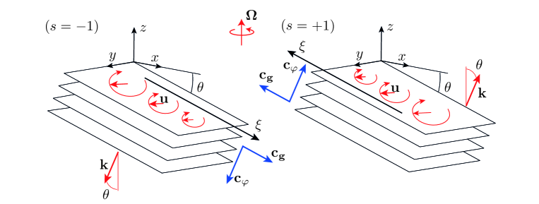
Figure 1: Sketch of a plane inertial wave of wavevector ${\bf k}$ with a polarity $s=-1$ (left) and $s=+1$ (right). The wave is invariant in the horizontal $y$-direction ($k_{y}=0$). The fluid motions consist in an anticyclonic circular translation in the planes of constant phase, normal to ${\bf k}$, which are tilted by an angle $\theta=\cos^{-1}(\sigma^{*})=\cos^{-1}(k_{z}/k)$ with respect to the horizontal. The phase of the wave propagates normally to these constant phase planes, but the energy of the wave propagates parallel to these planes along the group velocity. The vectors ${\bf c_{g}}$ and ${\bf c_{\varphi}}$ indicate the direction of the group and phase velocities, respectively. The amplitude of the fluid motions is damped along the energy propagation direction ${\bf c_{g}}$ at a rate $\nu k^{2}$.

The structure of a plane inertial wave of wavevector ${\bf k}$ is sketched in Fig. 1, for the two possible polarities $s=-1$ and $s=+1$. The fluid motions in the wave consist in an anticyclonic circular translation at frequency $\sigma=s2\Omega\,k_{z}/k$ in the planes of constant phase, which are normal to ${\bf k}$ and therefore tilted by an angle $\theta=\cos^{-1}(\sigma^{*})=\cos^{-1}(k_{z}/k)$ with respect to the horizontal ($k_{z}={\bf k}\cdot\hat{\bf z}$). The phase shift of the motion between close parallel planes of constant phase involves a shear and finally leads to a vorticity $\nabla\times{\bf u}$ that is parallel to the local velocity ${\bf u}$. The energy of the wave propagates parallel to the slope of the planes of constant phase at the group velocity $|{\bf c_{g}}|=2\Omega\sin\theta/k$. The energy goes upwards (with respect to $\hat{\bf z}$) when $s=+1$ and downwards when $s=-1$. The phase of the wave propagates at the phase velocity ${\bf c_{\varphi}}=\sigma{\bf k}/k^{2}$ which is normal to the planes of constant phase and therefore to the group velocity ${\bf c_{g}}$. Viscosity damps the wave amplitude as

$$\exp\left(-\frac{\nu k^{2}}{|{\bf c_{g}}|}\xi\right)=\exp\left(-\frac{\nu k^{3}}{2\Omega\sin\theta}\xi\right)$$ (3)

in the direction of the group velocity ${\bf c_{g}}$ at which the energy of the wave propagates Lighthill1967 ; Sutherland2010 ($\xi$ is the spatial coordinate in the direction of the group velocity, see Fig. 1).

II.2 The helical basis decomposition

Following Smith & Waleffe Smith1999 , we can decompose any divergence-free velocity field ${\bf u}({\bf x},t)$ on the basis of helical modes as

$${\bf u}({\bf x},t)=\sum_{\bf k}\sum_{s_{\bf k}=\pm 1}b_{s_{\bf k}}({\bf k},t){\bf h}_{s_{\bf k}}({\bf k})\,e^{i[{\bf k}\cdot{\bf x}-\sigma_{s_{\bf k}}({\bf k})t]}\,,$$ (4)

where $\sigma_{s_{\bf k}}({\bf k})$ is the angular frequency of the mode with wavevector ${\bf k}$, amplitude $b_{s_{\bf k}}({\bf k},t)$ and polarity $s_{\bf k}=\pm 1$. The helical base vectors ${\bf h}_{s_{\bf k}}({\bf k})$ are defined as

$${\bf h}_{s_{\bf k}}=\frac{\bf k}{|{\bf k}|}\times\frac{{\bf k}\times\hat{\bf z}}{|{\bf k}\times\hat{\bf z}|}+i\,s_{\bf k}\frac{{\bf k}\times\hat{\bf z}}{|{\bf k}\times\hat{\bf z}|}\,.$$ (5)

Inserting the decomposition (4) into the Navier-Stokes equation (1) yields a set of equations for the evolution of the amplitude $b_{s_{\bf k}}$ of the modes $({\bf k},s_{\bf k},\sigma_{s_{\bf k}})$

$$\left(\frac{\partial}{\partial t}+\nu k^{2}\right)b_{s_{\bf k}}=\frac{1}{2}\sum_{{\bf k}+{\bf p}+{\bf q}=\boldsymbol{0}}C_{{\bf k}{\bf p}{\bf q}}^{s_{\bf k}s_{\bf p}s_{\bf q}}\overline{b}_{s_{\bf p}}\,\overline{b}_{s_{\bf q}}e^{i(\sigma_{s_{\bf k}}+\sigma_{s_{\bf p}}+\sigma_{s_{\bf q}})t}\,,$$ (6)

due to non-linear interactions with couples of modes $({\bf p},s_{\bf p},\sigma_{s_{\bf p}})$ and $({\bf q},s_{\bf q},\sigma_{s_{\bf q}})$ (the overline indicates complex conjugate). In Eq. (6), the sum is taken over all wavevectors ${\bf p}$ and ${\bf q}$ such that ${\bf k}+{\bf p}+{\bf q}=\boldsymbol{0}$, and over the polarities $s_{\bf p}=\pm 1$, $s_{\bf q}=\pm 1$. The triadic interaction coefficients are defined as

$$C_{{\bf k}{\bf p}{\bf q}}^{s_{\bf k}s_{\bf p}s_{\bf q}}=\frac{s_{q}q-s_{p}p}{2}\,[{\overline{\bf h}}_{s_{p}}({\bf p})\times{\overline{\bf h}}_{s_{q}}({\bf q})]\cdot{\overline{\bf h}}_{s_{k}}({\bf k})\,,$$ (7)

where $p=|{\bf p}|$ and $q=|{\bf q}|$.

II.3 Triadic resonance of inertial waves

In Eqs. (4) and (6), if the frequency $\sigma_{s_{\bf k}}({\bf k})$ of a mode with wavevector ${\bf k}$ obeys the dispersion relation of inertial waves,

$$\sigma_{s_{\bf k}}({\bf k})=2\Omega\,s_{\bf k}\,\frac{k_{z}}{k}\,,$$ (8)

the resulting helical mode corresponds exactly to a plane inertial wave Smith1999 . To describe the triadic resonance instability of a plane inertial wave, we therefore restrict the system of equations (6) to three waves defined by $({\bf k_{0}},s_{0},\sigma_{0})$, $({\bf k_{1}},s_{1},\sigma_{1})$ and $({\bf k_{2}},s_{2},\sigma_{2})$. These three waves have frequencies that follow the dispersion relation (8) and that fulfill the triadic resonance conditions

$$\sigma_{0}+\sigma_{1}+\sigma_{2} = 0\,,$$ (9)

$${\bf k_{0}}+{\bf k_{1}}+{\bf k_{2}} = {\bf 0}\,.$$ (10)

The spatial resonance condition (10) was already included in Eq. (6). Then, writing the temporal resonance condition (9) amounts to assume that the flow is weakly non-linear, i.e., that the wave period $1/\sigma_{i}$ is much shorter than the non-linear time $1/(k_{i}b_{i})$, where $b_{i}$ is the amplitude of wave $i$ and $k_{i}=|{\bf k_{i}}|$. This weak non-linearity condition is achieved when the Rossby number of the waves, $Ro_{i}=b_{i}k_{i}/(4\pi\Omega)$, is small compared to the normalized wave period $\sigma_{i}^{*}=\sigma_{i}/2\Omega$, which implies that non-linear processes driving the evolution of the amplitudes $b_{i}(t)$ are slow compared to the wave oscillations. Under this weak non-linearity assumption, the dominant contributions to the right hand side term of Eq. (6) come from waves that meet the temporal resonance condition such that $e^{i(\sigma_{s_{\bf k}}+\sigma_{s_{\bf p}}+\sigma_{s_{\bf q}})t}=1$ Smith1999 ; Monsalve2020 . For non-resonant triads, the contribution of the complex exponential tends toward zero when integrated over times longer than $1/(\sigma_{s_{\bf k}}+\sigma_{s_{\bf p}}+\sigma_{s_{\bf q}})$, strongly reducing the efficiency of the energy exchanges within the triad Galtier2003 ; Nazarenko2011 . Although these arguments suggest that only resonant triads are of interest, this is strictly true only at vanishing Rossby number and recent works have shown that near-resonant LeReun2020 and even non-resonant Brunet2020 triads can trigger instabilities of inertial waves toward 2D vertically invariant modes at finite Rossby number, these instabilities having however growth rates $Ro$ times smaller than of the triadic resonance instability.

II.4 Instability growth rate

In the following, we consider that the flow is composed of a plane inertial wave (labelled $0$), as the base flow, and two secondary plane inertial waves (labelled $1$ and $2$) that result from the instability. Without loss of generality, we choose the primary wave $0$ to be invariant in the $y$-direction, i.e., that ${\bf k_{0}}=(k_{x,0},0,k_{z,0}$), to have a positive angular frequency $\sigma_{0}$, and a negative polarity $s_{0}=-1$. We also consider the case (corresponding to the experiments presented later) where $k_{x,0}<0$, $k_{z,0}$ being negative as a consequence of the dispersion relation. We restrict our analysis to the early development of the instability, assuming that the primary wave amplitude $b_{0}$ remains constant and the amplitudes of the secondary waves, $b_{1}$ and $b_{2}$, remain small compared to $b_{0}$, a situation sometimes called the “pump-wave approximation” Craik1978 ; Gururaj2020 . Following (6), the evolution of the amplitudes of the secondary waves is described by

$$\frac{db_{1}}{dt}=C_{1}\overline{b}_{0}\overline{b}_{2}-\nu k_{1}^{2}b_{1}\,,$$ (11)

$$\frac{db_{2}}{dt}=C_{2}\overline{b}_{0}\overline{b}_{1}-\nu k_{2}^{2}b_{2}\,,$$ (12)

where $k_{1}=|{\bf k_{1}}|$, $k_{2}=|{\bf k_{2}}|$, $C_{1}=C_{{\bf k_{1}}{\bf k_{0}}{\bf k_{2}}}^{s_{\bf k_{1}}s_{\bf k_{0}}s_{\bf k_{2}}}$ and $C_{2}=C_{{\bf k_{2}}{\bf k_{1}}{\bf k_{0}}}^{s_{\bf k_{2}}s_{\bf k_{1}}s_{\bf k_{0}}}$. Solving this system of equations leads to an exponential growth (or decay) of $b_{1}$ and $b_{2}$ at a rate

$$\gamma=\frac{-\nu(k_{1}^{2}+k_{2}^{2})}{2}+\sqrt{\frac{\nu^{2}(k_{1}^{2}-k_{2}^{2})^{2}}{4}+C_{1}\overline{C_{2}}|b_{0}|^{2}}\,,$$ (13)

the product $C_{1}\overline{C_{2}}$ being real. We first note that the instability growth rate $\gamma$ does not depend on the rotation rate of the fluid $\Omega$. Thus, $\gamma$ will depend on the primary wave Reynolds number $Re_{0}=b_{0}2\pi/(k_{0}\nu)$ and on its non-dimensional frequency $\sigma_{0}^{*}$ but not on the primary wave Rossby number $Ro_{0}=b_{0}k_{0}/(4\pi\Omega)$.

In the inviscid limit where the primary wave Reynolds number tends to infinity, the expression of the instability growth rate reduces to $\gamma=|b_{0}|\sqrt{C_{1}\overline{C_{2}}}$. In this situation, and in the 2D case where secondary waves propagates in the same vertical plane as the primary wave (i.e. $k_{y,1}=k_{y,2}=0$), the maximum growth rate is found for secondary wavenumbers much larger than the primary wavenumber such that ${\bf k_{1}}\simeq-{\bf k_{2}}$ Staquet2002 ; Koudella2006 ; Bordes2012 . As a consequence, the secondary waves are found at degenerated frequencies $|\sigma_{1}|\simeq|\sigma_{2}|$ equal to half the primary wave frequency $\sigma_{0}/2$ and the TRI is often called parametric subharmonic instability (PSI) Staquet2002 ; Koudella2006 ; Bordes2012 .

Building on several identities pointed out in Waleffe1992 ; Smith1999 (see Appendix A), the inviscid growth rate can in the general 3D case be rewritten as

$$\gamma=|b_{0}|\left[\frac{\sin^{2}\alpha_{2}}{4k_{2}^{2}}\left(s_{0}k_{0}+s_{1}k_{1}+s_{2}k_{2}\right)^{2}\frac{\sigma_{1}\sigma_{2}}{\sigma_{0}^{2}}\left(s_{2}k_{2}-s_{1}k_{1}\right)^{2}\right]^{1/2}\,,$$ (14)

where $\alpha_{2}$ is the angle opposite to the side ${\bf k_{2}}$ in the closed triangle formed by the resonant triads $({\bf k_{0}},{\bf k_{1}},{\bf k_{2}})$.

We assume in the following of this subsection II.4 that, in the inviscid 3D case, the secondary wavenumbers associated to the maximum growth rate are also much larger than the primary wavenumber such that $|\sigma_{1}|=|\sigma_{2}|=\sigma_{0}/2$ and $k_{1}\simeq k_{2}\gg k_{0}$ (this assumption will be validated in the next subsection). Focusing on the combination of wave polarities $(s_{0}=-1,s_{1}=+1,s_{2}=-1)$, an asymptotic expansion of the growth rate to the first order in $k_{0}/k_{1}\simeq k_{0}/k_{2}$ leads to a simple expression for the growth rate depending only on the angle $\alpha_{2}$ (see Appendix A)

$$\frac{\gamma}{k_{0}|b_{0}|}\simeq\frac{1}{2}\sin\alpha_{2}\left(1-\cos\alpha_{2}\right)\,.$$ (15)

Maximizing this expression with respect to the angle $\alpha_{2}$, the maximum growth rate $\gamma^{(\rm max)}/(k_{0}|b_{0}|)\simeq 0.6495$ is found for the specific angle $\alpha_{2}=2\pi/3$ (120^∘) independently of the primary wave frequency $\sigma_{0}^{*}$.

Remarkably, this angle $\alpha_{2}=2\pi/3$ can only be found for 3D resonant triads with the secondary waves propagating in other vertical planes than the one of the primary wave, i.e., with a non-zero $y$-component of their wavevectors $k_{y,1}=-k_{y,2}$. More precisely, we show in Appendix A that

$$\frac{k_{y,1}}{k_{x,1}}=\pm\left(\frac{3}{1-{\sigma^{*}_{0}}^{2}}\right)^{1/2}\,.$$ (16)

For the primary wave non-dimensional frequency that will further be considered in our experiments, $\sigma_{0}^{*}=0.84$, this corresponds to an angle

$$\phi_{1}=\tan^{-1}\left(\frac{3}{1-{\sigma^{*}_{0}}^{2}}\right)^{1/2}\simeq 73^{\circ}$$ (17)

between the vertical plane of propagation of the primary wave and the one of secondary wave $1$ (and secondary wave $2$ actually). For $\sigma_{0}^{*}$ ranging from $0$ to $1$, the angle $\phi_{1}$ ranges from $60^{\circ}$ to $90^{\circ}$. This result is remarkable: It demonstrates that, in the inviscid limit, the most unstable triad is always three dimensional with secondary waves propagating in vertical planes making an angle between $60^{\circ}$ and $90^{\circ}$ with the primary wave vertical plane of propagation.

In the following, we come back to the general 3D case with viscosity and identify numerically the maximum growth rate of the instability.

II.5 Instability growth rate in the viscous case

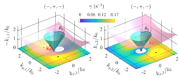
Figure 2: Resonance surfaces of ${\bf k_{1}}$ (left) and ${\bf k_{2}}$ (right) for the combination of wave polarities $(-,+,-)$ and a primary wave defined by ($k_{0}=0.83$ rad/cm, $s_{0}=-1$, $\sigma_{0}^{*}=0.84$, $b_{0}=0.39$ cm/s). In the left panel, the vertical axis shows $-k_{z,1}$ for sake of clarity. The two 3D plots also show the cone of apex at ${\bf k_{i}}={\bf 0}$ and of semi-angle $\theta_{0}=\cos^{-1}(\sigma_{0}^{*})$. This cone represents the waves at the forcing frequency according to the dispersion relation. Below each resonance surface, we also report the map of the growth rate $\gamma$ of the instability in the plane ($k_{x,i},k_{y,i}$) in which the locations of the maximum growth rate are shown by black dots. The value $\nu=1.20\times 10^{-6}$ m²/s is used for the kinematic viscosity in order to match the experimental value in the next section.

In Fig. 2, we report in the coordinate system ($k_{x}/k_{0},k_{y}/k_{0},k_{z}/k_{0}$) the “resonance surfaces” defined by all the wavevectors ${\bf k_{1}}$ (left) and ${\bf k_{2}}$ (right) which are solutions of the triadic resonance conditions (9-10). These surfaces are computed for a primary wave defined by ($k_{0}=0.83$ rad/cm, $s_{0}=-1$, $\sigma_{0}^{*}=0.84$, $b_{0}=0.39$ cm/s), and for a combination of wave polarities $(s_{0}=-1,s_{1}=+1,s_{2}=-1)$ denoted in the following by the short-hand $(-,+,-)$. These resonance surfaces illustrate all the possible couples of secondary waves (${\bf k_{1}},{\bf k_{2}=\bf k_{0}-\bf k_{1}}$) in triadic resonance with the primary wave for the case $(-,+,-)$. These resonance surfaces are the three-dimensional extensions of the 2D classical resonance curves, reported in several works Smith1999 ; Koudella2006 ; Joubaud2012 ; Bordes2012 , which are restricted to secondary waves invariant in the $y$-direction ($k_{y}=0$), as the primary wave. Below each resonance surface, we report the map of the corresponding growth rate $\gamma$ of the instability (13) in the plane ($k_{x,i},k_{y,i}$). The primary wave Reynolds number is $Re_{0}=b_{0}2\pi/(k_{0}\nu)\simeq 245$ where the value $\nu=1.20\times 10^{-6}$ m²/s is used for the kinematic viscosity in order to match the experimental value in the next section. The rotation rate $\Omega=18$ rpm is the same as the one of the experiments presented later in the article. It yields a primary wave Rossby number of $Ro_{0}=b_{0}k_{0}/(4\pi\Omega)\simeq 0.014$.

The left panel of Fig. 2 shows the resonance surface for the wavevector ${\bf k_{1}}$ (note that the vertical axis reports $-k_{z,1}$ for sake of clarity). This resonance surface (in pink) extends up to infinity, with any choice of the wavevector components ($k_{x,1},k_{y,1}$) having a resonant solution. The resonance surface uniformly lies below the cyan cone of apex at ${\bf k_{1}}={\bf 0}$ [a point also included in the resonance surface] and semi-angle $\theta_{0}=\cos^{-1}(\sigma_{0}^{*})$ corresponding to wavevectors ${\bf k_{1}}$ of waves at the forcing frequency according to the dispersion relation. This observation means that the resonant secondary waves $1$ always have a wavevector ${\bf k_{1}}$ which is more horizontal than the primary wavevector ${\bf k_{0}}$ (shown in the figure). According to the dispersion relation (2), it implies that $|\sigma_{1}|<|\sigma_{0}|$. We also note that a small portion of the ${\bf k_{1}}$ resonance surface associated to positive values of $k_{z,1}$ and small values of ($k_{x,1},k_{y,1}$) is not shown. One can however see that this range of secondary wavevectors ${\bf k_{1}}$ is associated with a negative growth rate $\gamma$ and is therefore not to be further considered.

The right panel of Fig. 2 shows the resonance surface for the wavevector ${\bf k_{2}}={\bf k_{0}}-{\bf k_{1}}$. Although this information is equivalent to the one found on the left panel, the ${\bf k_{2}}$ resonance surface highlights interesting features. For instance, contrary to the case of ${\bf k_{1}}$, the ${\bf k_{2}}$ resonance surface does not intersect the $k_{z}=0$ plane since $k_{z,2}$ is always strictly positive. In addition, a portion of the resonance surface at small ($k_{x,2},k_{y,2}$) lies inside the cone of semi-angle $\theta_{0}=\cos^{-1}(\sigma_{0}^{*})$. One can see in the map of $\gamma$ reported in the plane ($k_{x,2},k_{y,2}$) that the corresponding values of ${\bf k_{2}}$ are however associated with the regime of negative growth rate already noticed in the left panel for the wavevector ${\bf k_{1}}$. Again, if we restrict our analysis to positive growth rates $\gamma$, the secondary wavevectors ${\bf k_{2}}$ are more horizontal than the primary wavevector ${\bf k_{0}}$. In summary, the resonant secondary waves $1$ and $2$ have frequencies that are always smaller in absolute value than the one of the primary wave, $|\sigma_{1,2}|<|\sigma_{0}|$, i.e., the secondary wavevectors ${\bf k_{1}}$ and ${\bf k_{2}}$ are always more horizontal than the primary wavevector Smith1999 . Considering that in the present conventions frequencies can be negative, a resonant triad with a primary wave of positive frequency $\sigma_{0}$ will have negative frequencies for both secondary waves obeying the relation $|\sigma_{1}|+|\sigma_{2}|=|\sigma_{0}|$.

We now come to the most important conclusion of this section: the growth rate of the instability $\gamma$ is maximum for secondary waves which are not propagating in the same plane as the primary wave, i.e., for secondary waves that are not invariant in the $y$-direction ($k_{y}\neq 0$). The triadic resonance instability of a plane inertial wave is therefore expected to be a three-dimensional instability transferring energy to secondary waves with a wavevector component $k_{y}$ of the same order as $k_{x}$. This can be observed in Fig. 2, where the two locations of the maximum growth rate in the ($k_{x,i},k_{y,i}$)-planes are indicated by black dots. There are actually two couples of secondary waves that maximize the growth rate with symmetric wavevectors ${\bf k_{i}}$ with respect to the primary wave vertical plane $k_{y,i}=0$. In the sequel, we will show that this three-dimensionality is in agreement with the experiments.

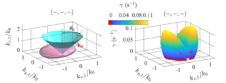
Figure 3: Resonance surface of ${\bf k_{1}}$ (left, in pink) and 3D view of the instability growth rate $\gamma$ (right) for the combination of polarities $(-,-,-)$. In the left panel, we also show the cone of apex at ${\bf k_{1}}={\bf 0}$ and of semi-angle $\theta_{0}=\cos^{-1}(\sigma_{0}^{*})$. The surfaces are computed for a primary wave defined by ($k_{0}=0.83$ rad/cm, $s_{0}=-1$, $\sigma_{0}^{*}=0.84$, $b_{0}=0.39$ cm/s) in a rotating fluid of kinematic viscosity $\nu=1.20\times 10^{-6}$ m²/s.

For the sake of completeness, we also consider the combinations of polarities $(-,-,+)$ and $(-,-,-)$. The first combination, $(-,-,+)$ is actually the same case as $(-,+,-)$ where the roles of the waves $1$ and $2$ have been exchanged. For the polarities combination $(-,-,-)$, Fig. 3 shows the resonance surface for ${\bf k_{1}}$ on the left and a 3D view of the corresponding growth rate $\gamma$ as a function of ($k_{x,1},k_{y,1}$) on the right. This representation is necessary since the resonance surface is a closed surface with values of $k_{1}$ of the order of $k_{0}$. This implies that for a given couple of wavevector components ($k_{x,1},k_{y,1}$) there are either two resonant solutions for $k_{z,1}$ at small ($k_{x,1},k_{y,1}$) or no solution at large ($k_{x,1},k_{y,1}$). Then, $\gamma$ takes also two values when $k_{z,1}$ does. As for the $(-,+,-)$ instability, when the instability growth rate $\gamma$ is positive, the secondary waves are subharmonic with $|\sigma_{1}|$ and $|\sigma_{2}|$ smaller than $|\sigma_{0}|$. On the contrary, the maximum growth rate of the instability is this time found for secondary waves with $k_{y}=0$, invariant along the $y$-direction. At the considered non-dimensional frequency $\sigma_{0}^{*}=0.84$, the $(-,-,-)$ instability is therefore 2D to the first order, i.e., if one considers only its maximum growth rate.

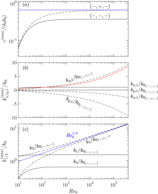
Figure 4: (a) Maximum normalized instability growth rate $\gamma^{\rm(max)}/(k_{0}b_{0})$ for polarities combinations $(-,+,-)$ and $(-,-,-)$ as a function of the primary wave Reynolds number $Re_{0}=b_{0}2\pi/(\nu k_{0})$ for $\sigma_{0}^{*}=0.84$. The horizontal blue straight line reports the value $\gamma^{\rm(max)}/(k_{0}b_{0})$ predicted analytically in the inviscid limit in the previous section II.4 (see Eq. 15). (b) Wavevector components $k_{x,1}^{\rm(max)}$ and $k_{y,1}^{\rm(max)}$ corresponding to the maximum growth rate for each mode as a function of $Re_{0}$ (again for $\sigma_{0}^{*}=0.84$). The red curve shows the wavenumber $\sqrt{3/(1-{\sigma_{0}^{*}}^{2})}\,|k_{x,1}^{\rm(max)}|$ which is predicted in the inviscid limit (see section II.4) to match the wavevector component $k_{y,1}^{\rm(max)}$ for the instability mode $(-,+,-)$. (c) Corresponding wavenumbers. The blue straight line shows a power law $Re_{0}^{1/4}$.

To conclude this section, we report in Fig. 4(a) the evolution of the maximum instability growth rate $\gamma^{\rm(max)}$ for combinations $(-,+,-)$ and $(-,-,-)$ as a function of the primary wave Reynolds number $Re_{0}=b_{0}2\pi/(\nu k_{0})$ for $\sigma_{0}^{*}=0.84$. This maximum growth rate is actually shown normalized by the non-linear frequency of the primary wave as $\gamma^{\rm(max)}/(k_{0}b_{0})$. The normalized maximum growth rate naturally grows with $Re_{0}$ for both modes starting from vanishing and asymptotically equal values at small $Re_{0}$. At large $Re_{0}$, the normalized growth rate $\gamma^{\rm(max)}/(k_{0}b_{0})$ tends toward order $1$ asymptotic values, the growth rate for the $(-,+,-)$ mode being typically twice larger than for the $(-,-,-)$ mode. Moreover, in the $(-,+,-)$ case, the maximum normalized growth rate tends toward the inviscid value $\gamma^{(\rm max)}/(k_{0}b_{0})\simeq 0.6495$ predicted analytically in the previous section II.4 (see Eq. 15). In Fig. 4(b), we show the wavevector components $k_{x,1}^{\rm(max)}$ and $k_{y,1}^{\rm(max)}$ corresponding to the maximum growth rate for each mode and as a function of $Re_{0}$ (again for $\sigma_{0}^{*}=0.84$). For the instability mode $(-,+,-)$, $k_{x,1}^{\rm(max)}$ is negative and slowly grows in absolute value from $\sim k_{0}/10$ at $Re_{0}\simeq 10$ up to $\sim 2.7\,k_{0}$ at $Re_{0}\simeq 4\times 10^{5}$ whereas $k_{y,1}^{\rm(max)}$ can take two opposite values that grow in absolute value from $\sim k_{0}/10$ at $Re_{0}\simeq 10$ to $\sim 9.3\,k_{0}$ at $Re_{0}\simeq 4\times 10^{5}$, in agreement with the symmetry found in Fig. 2. We also report in Fig. 4(b) as a red curve the wavenumber $|k_{x,1}^{\rm(max)}|\,\sqrt{3/(1-{\sigma_{0}^{*}}^{2})}$ which is predicted in the inviscid limit (see section II.4) to match the wavevector component $k_{y,1}^{\rm(max)}$. One can observe that the value of $k_{y,1}^{\rm(max)}$ numerically obtained from the full set of viscous equations is actually already close to its inviscid prediction at moderate $Re_{0}$. The behavior of the mode $(-,-,-)$ is very different. The maximum-growth-rate instability is 2D, with $k_{y,1}^{\rm(max)}=0$ for all $Re_{0}$, and $k_{x,1}^{\rm(max)}$ positive, of order $k_{0}$ and slowly increasing with $Re_{0}$. Figure 4(c) finally shows that for the $(-,+,-)$ mode the norm of the subharmonic wavenumbers, $k_{1}$ and $k_{2}$, continuously grows from values of the order of $\sim 0.3\,k_{0}$ and $\sim 1.4\,k_{0}$ at $Re_{0}\simeq 10$, respectively, up to values of the order of $\sim 13\,k_{0}$ at $Re_{0}\simeq 4\times 10^{5}$. At large $Re_{0}$, $k_{1}/k_{0}$ and $k_{2}/k_{0}$ increase following power laws $Re_{0}^{1/4}$. In parallel, for the $(-,-,-)$ mode, $k_{1}$ and $k_{2}$ slowly grow over the considered range of Reynolds number while remaining in the range between $0.3\,k_{0}$ and $1.5\,k_{0}$.

The previous theoretical developments demonstrate the 3D character of the TRI of a plane inertial wave. In the sequel, we explore this question from an experimental point of view before we finally compare the two approaches quantitatively.

III Experimental setup

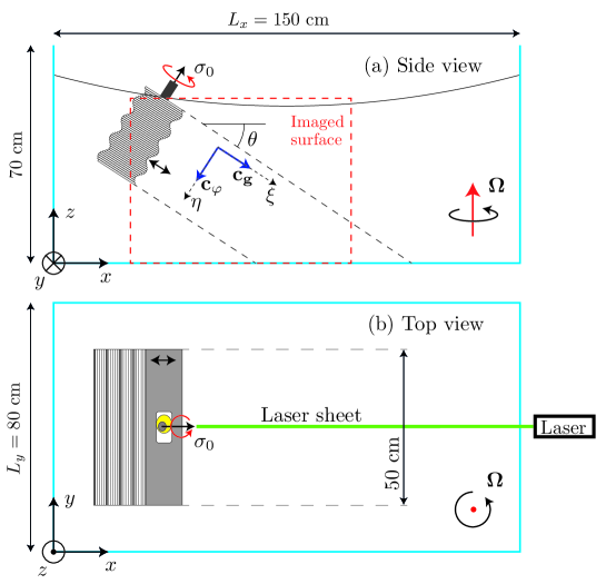
Figure 5: Sketch of the experimental setup seen from the side (a) and from the top (b).

The flow is generated in a parallelepipedic glass tank of $L_{x}\times L_{y}=150\times 80$ cm² rectangular base and $70$ cm height filled with $55$ cm of water as sketched in Fig. 5. A plane inertial wave is forced in the tank by an immerged wave maker which has already been implemented in several studies of internal gravity waves in stratified fluids Joubaud2012 ; Scolan2013 ; Bourget2013 ; Brouzet2017 and in a previous study of the instability of a plane inertial wave Bordes2012 . A major difference with these previous experiments has nevertheless been introduced : the wake maker produces here a plane wave with a large spatial extension in the horizontal direction $y$ (in which the forced wave is supposed to be invariant) normal to the wave propagation plane ($x,z$). More precisely, the wave maker extent in the $y$-direction is of $50$ cm whereas it was of $14$ cm in the previous studies, these lengths being to be compared to the forced wavelength of $7.6$ cm.

The wave maker is composed of a stack of $48$ plates which are $6.33$ mm thick and $50$ cm wide (see Fig. 5). The plates are fitted with a rectangular hole at their center through which a camshaft is inserted, each cam being a circular plate adjusted to the hole with a rotation point shifted from its center by an eccentricity $A$ (scotch yoke mechanism). A constant angular shift of $30$ degrees is introduced between adjacent cams leading the surface drawn by the plate edges to approximate a sinusoidal shape of wavelength $\lambda_{f}=7.6$ cm. The profile contains four wavelengths such that the produced wave beam will have a $4\lambda_{f}=30.4$ cm width. A brushless motor coupled to a reducer is driving the camshaft in a constant rotation at an angular frequency $\sigma_{0}$ such that each plate is finally subject to an oscillating linear translation motion in the direction normal to its width and to the camshaft axis (the plates are guided laterally). The wave maker surface eventually describes a sinus profile

$$\xi_{\rm wm}(\eta,t)=A\sin(\sigma_{0}t-k_{0}\eta)\,,$$ (18)

with a phase propagating downward, parallel to the camshaft axis. In Eq. (18), $k_{0}=2\pi/\lambda_{f}$ is the wavenumber, $\eta$ is the coordinate along the phase propagation direction and $\xi$ the coordinate along the energy propagation direction (see Fig. 5).

The whole system is mounted on a $2$-m diameter platform rotating at a rate $\Omega=18$ rpm. The angular frequency of the wave maker is set to $\sigma_{0}=0.84\times 2\Omega\simeq 3.17$ rad/s. Following the inertial wave dispersion relation, the wave maker is tilted at an angle $\theta_{0}=\cos^{-1}(\sigma_{0}/2\Omega)\simeq 32.9^{\circ}$ with its deforming surface pointing downwards. With this tilt, the motion of the wave maker surface matches the velocity boundary condition of a plane inertial wave at frequency $\sigma_{0}$ and propagating downwards (polarity $s_{0}=-1$). More precisely, the wave maker drives inertially the velocity component of the plane wave along its energy propagation direction (axis $\xi$ in Fig. 5) without however forcing the velocity component along the wave invariance direction $y$. Given the location of the wave maker in the tank (Fig. 5), the forced wave will propagate over a distance of about $60$ cm before the reflection on the bottom of the tank takes place. In our study, we use cams with eccentricity $A$ equal to either $1$, $1.5$ or $2$ mm, leading to forcing Reynolds numbers $Re_{f}=A\sigma_{0}\lambda_{f}/\nu$ in the range $230\leq Re_{f}\leq 420$ and forcing Rossby numbers $Ro_{f}=A\sigma_{0}/(2\Omega\lambda_{f})$ in the range $0.011\leq Ro_{f}\leq 0.022$.

The two components $(u_{x},u_{z})$ of the velocity field are measured in the vertical plane $y=y_{0}=L_{y}/2$ using a particle image velocimetry (PIV) system mounted in the rotating frame ($y=0$ is the front side of the tank). The water is seeded with $10$ $\mu$m tracer particles and illuminated by a laser sheet generated by a corotating 140 mJ Nd:YAG pulsed laser. For each experiment, $7\,920$ images of particles are acquired using a $2\,360\times 1\,776$ pixels camera at a frequency of $24$ images per wave maker period $T=2\pi/\sigma_{0}$. The acquisition, which is started $30$ forcing periods before the start of the wave maker, covers $330$ periods in total. The imaged region has a surface of $71\times 53$ cm² (see the dashed rectangle in Fig. 5). PIV cross-correlation is finally performed between successive images using $32\times 32$ pixels interrogation windows with a $50\%$ overlap and provides velocity fields with a spatial resolution of $4.8$ mm. The rotation of the platform is always started at least $30$ min before the start of the wave maker in order for the spin-up of the fluid to be completed.

IV Experimental results

IV.1 Subharmonic instability

In order to explore the temporal content of the flow produced by the wave maker, we compute the temporal power spectral density of the measured velocity field as

$$E(\sigma,t,\Delta T)=\frac{4\pi}{\Delta T}\langle|\widetilde{\mathbf{u}}(x,z,\sigma,t,\Delta T)|^{2}\rangle$$ (19)

where the components of $\widetilde{\mathbf{u}}$ are given by

$$\widetilde{u}_{j}(x,z,\sigma,t,\Delta T)=\frac{1}{2\pi}\int_{t-\Delta T/2}^{t+\Delta T/2}u_{j}(x,y_{0},z,t^{\prime})e^{-i\sigma t^{\prime}}dt^{\prime}\,,$$ (20)

the temporal Fourier transform of the velocity component $u_{j}(x,y_{0},z,t)$ with $j=(x,z)$ and the angular brackets denote the spatial average over the measurement area in the plane $y_{0}=L_{y}/2$.

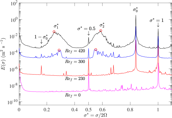
Figure 6: Temporal power spectral density $E(\sigma,t=150\,T,\Delta T=300\,T)$ as a function of the normalized frequency $\sigma^{*}=\sigma/2\Omega$ for experiments at $\sigma_{0}^{*}=0.84$ and $\Omega=18\leavevmode\nobreak\$rpm for a forcing wavelength $\lambda_{f}=7.6$ cm and four forcing Reynolds numbers, $Re_{f}=0$ (pink curve), $Re_{f}=230$ (red), $300$ (blue) and $420$ (black). The spectrum at $Re_{f}=0$ corresponds to an experiment with the wave generator off. A vertical shift by a factor of $20$ has been introduced between successive spectra.

In Fig. 6, we report the temporal spectra $E(\sigma,t,\Delta T)$ as a function of the normalized frequency $\sigma^{*}=\sigma/2\Omega$ for the three experiments at forcing amplitudes $A=1,1.5$ and $2$ mm. The Fourier transform (20) is computed over the whole experimental duration from the start of the wave maker ($\Delta T=300\,T$, $t=\Delta T/2$, $T=2\pi/\sigma_{0}$ being the period of the forcing). As a reference, we also report a spectrum measured with the wave generator off ($A=0$ and $Re_{f}=0$). All the spectra (with the wave generator on) exhibit an energetically dominant peak at the driving frequency $\sigma_{0}^{*}=0.84$. The spectrum at the lowest (non-zero) forcing amplitude (Reynolds number $Re_{f}=230$) corresponds to a flow in the linear regime, below the onset of the triadic resonance instability. Nevertheless, secondary peaks at frequencies $\sigma=\Omega$ ($\sigma^{*}=0.5$), $\sigma=2\Omega$ ($\sigma^{*}=1$) and $\sigma=2\Omega-\sigma_{0}$ ($\sigma^{*}=0.16$) are observed. One can note that the energy peaks at $\sigma=\Omega$ ($\sigma^{*}=0.5$) and $\sigma=2\Omega$ ($\sigma^{*}=1$) are already present, with the same amplitude, in the spectrum without forcing ($Re_{f}=0$). The peak at $\sigma=\Omega$ ($\sigma^{*}=0.5$) has actually been shown to correspond mainly to a flow created by the rotating platform’s precession induced by the Earth’s rotation (see Boisson2012 ; Triana2012 ). Nevertheless, we cannot exclude that part of the energy in this peak is related to mechanical perturbations of the system rotation at the frequency $\sigma=\Omega$ inducing inertial waves in the flow. The peak at $\sigma^{*}=1$ is the result of a perturbation of the platform rotation inducing waves at $\sigma=2\Omega$ in the water tank. The peak at $\sigma=2\Omega-\sigma_{0}$ ($\sigma^{*}=0.16$) can be interpreted as the result of the interaction between the mode at $\sigma=2\Omega$ and the forcing. We also observe a peak at $\sigma^{*}=0$ with a tail extending up to $\sigma^{*}\simeq 0.05$. This peak, already present with a similar amplitude in the spectrum without forcing, has already been discussed in Refs. Bordes2012 ; Brunet2019 and is due to the presence of thermal convection columns drifting horizontally in the water tank. Finally, other even weakly energetic peaks are present in the spectrum at $Re_{f}=230$ corresponding to direct combinations (sums and differences) of the frequencies of the leading energetic modes at $\sigma=\sigma_{0}$, $\sigma=\Omega$, $\sigma=2\Omega$. As one can see, these modes are progressively drowned in the spectral noise for the experiments conducted at larger forcing amplitudes.

When increasing the forcing Reynolds number to $Re_{f}=300$, two spectral bumps at subharmonic frequencies emerge. These bumps are almost perfectly symmetric with respect to half the forcing frequency $\sigma_{0}/2$, which indicates that the frequencies associated with these two bumps are in triadic resonance with the primary wave frequency $\sigma_{0}$. This observation is the classical signature of the triadic resonance instability of an inertial wave, and it has been widely reported in experimental Bordes2012 ; LeReun2019 ; Brunet2019 ; Brunet2020 ; Monsalve2020 and numerical works Jouve2014 ; LeReun2020 . As the forcing Reynolds number increases to $420$, the subharmonic bumps are spreading in frequency in agreement with previous experimental works Brunet2019 ; Brunet2020 . This latter feature is at odds with the subharmonic peaks observed in numerical simulations of a 2D inertial wave attractor by Jouve and Ogilvie Jouve2014 where the flow is strictly invariant in the transverse horizontal direction $y$. A possible explanation is that the large frequency width observed here for the subharmonic bumps produced by the TRI is a consequence of the three-dimensionality of the TRI allowed in the experiments but forbidden in the 2D simulations. Nevertheless, one cannot exclude that part of the spreading of the TRI subharmonic bumps observed here at $Re_{f}=420$ is the consequence of the emergence of secondary triadic resonant interactions in the flow, which could stand as the premises of a transition toward an inertial wave turbulence following the scenario reported in Monsalve2020 .

To further explore the characteristics of the secondary waves produced by the triadic resonance instability, we select, for each couple of subharmonic bumps, the angular frequency $\sigma_{1}^{*}$ associated to the maximum spectral density of the lowest-frequency bump in the spectra of Fig. 6. We report these values in Table 1 and highlight them in Fig. 6. Then, we select the frequency $\sigma_{2}^{*}=\sigma_{0}^{*}-\sigma_{1}^{*}$ in triadic resonance with $\sigma_{1}^{*}$. For each couple of bumps, we can see in Fig. 6 that the computed value $\sigma_{2}^{*}$ is very close to the frequency associated to the maximum of the second spectral bump ($\sigma_{1}^{*}$ and $\sigma_{2}^{*}$ are shown in Fig. 6 by red circles).

	Experiment #1	Experiment #2	Experiment #3
$Re_{f}$	230	300	420
$Ro_{f}$	0.011	0.017	0.022
$A$ (mm)	1	1.5	2.0
$\nu$ (m${}^{2}/$s)	$1.05\times 10^{-6}$	$1.20\times 10^{-6}$	$1.15\times 10^{-6}$
$\sigma_{1}^{*}$	no TRI	0.285	0.252
$\sigma_{2}^{*}=\sigma_{0}^{*}-\sigma_{1}^{*}$	no TRI	0.555	0.588
$k_{x,1}$ (rad/cm)	no TRI	$0.640\pm 0.104$	$0.625\pm 0.110$
$k_{y,1}$ (rad/cm)	no TRI	$1.314\pm 0.313$	$0.794\pm 0.125$
$k_{z,1}$ (rad/cm)	no TRI	$0.435\pm 0.097$	$0.263\pm 0.043$
$k_{x,2}$ (rad/cm)	no TRI	$-1.124\pm 0.145$	$-1.057\pm 0.120$
$k_{y,2}$ (rad/cm)	no TRI	$-1.188\pm 0.125$	$-0.729\pm 0.070$
$k_{z,2}$ (rad/cm)	no TRI	$-1.091\pm 0.127$	$-0.934\pm 0.058$

Table 1: Table reporting for each experiment the normalized frequency $\sigma_{1}^{*}$ associated to the maximum of the bump at the lowest frequency in each subharmonic couple and the associated resonant frequency $\sigma_{2}^{*}=\sigma_{0}^{*}-\sigma_{1}^{*}$ ($\sigma_{0}^{*}=\sigma_{0}/2\Omega=0.84$). These frequencies are highlighted by red circles in Fig. 6. The table also report for each subharmonic mode the values computed in section IV.2 of the wavevector components with the corresponding error bars. The forcing Reynolds and Rossby numbers are defined as $Re_{f}=A\sigma_{0}\lambda_{f}/\nu$ and $Ro_{f}=A\sigma_{0}/(2\Omega\lambda_{f})$, respectively. $\nu$ is the experimental kinematic viscosity of water (derived from temperature measurements), $\Omega=18$ rpm is the global rotation rate, $\sigma_{0}$ the forcing frequency, $A$ the forcing amplitude, and $\lambda_{f}=7.6$ cm the forcing wavelength.

In the following, we use a Hilbert filtering procedure to extract the velocity field associated with the modes at frequencies $\sigma_{1}$ and $\sigma_{2}$. This procedure consists in a band-pass Fourier filter of the velocity field at the frequency of interest $\sigma_{i}$ (with a band width equal to the spectral resolution) in conjunction with a filtering in the wavevector space retaining only the energy present in one (judiciously chosen) quadrant of the wavevector space ($k_{x},k_{z}$). Compared to a simple temporal Fourier filtering, this procedure allows us to remove other wave beams at the frequency of interest coming from reflections on the water tank boundaries, which have wavevectors components in the other three quadrants of the wavevector space. Moreover, the temporal filtering retains only the energy at the selected frequency $\sigma_{i}>0$ without including the corresponding negative frequency. This procedure leads to a complex velocity field whose real part is the physical field (once multiplied by $2$ to compensate the discarded negative frequency and enforce energy conservation) and whose argument $\varphi({\bf x})$ is the phase field of the wave of interest at the frequency $\sigma_{i}$. Details on this filtering procedure can be found in Refs. Bordes2012 ; Brunet2019 ; Mercier2008 .

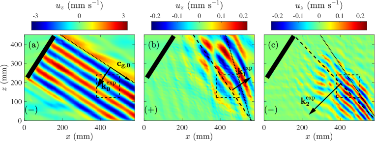
Figure 7: Snapshots of the vertical velocity component computed with the Hilbert filtering procedure for the experiment at $Re_{f}=300$ for frequencies $\sigma_{0}^{*}$, $\sigma_{1}^{*}$ and $\sigma_{2}^{*}$, respectively. (a) Temporal filter at $\sigma_{0}^{*}=0.84$ and spatial filter keeping the wavevector quadrant ($k_{x}<0,k_{z}<0$); (b) $\sigma_{1}^{*}=0.285$ and ($k_{x}>0,k_{z}>0$); (c) $\sigma_{2}^{*}=0.555$ and ($k_{x}<0,k_{z}<0$). In each panel, the dotted line indicates the theoretical tilt angle $\theta_{i}=\cos^{-1}(\sigma_{i}^{*})$ with the horizontal predicted for the constant phase planes for a wave at the considered frequency $\sigma_{i}^{*}$ and propagating in the vertical measurement plane ($x,z$), i.e. with $k_{y}=0$. The black rectangle (more precisely its underside) indicates the mean position of the wave generator surface. In (b) and (c), the dashed line indicates the direction normal to the projection in the measurement plane of the wavevectors computed in Sec. IV.2 for the modes at $\sigma_{1}^{*}$ and $\sigma_{2}^{*}$ in the instability region (dashed rectangle).

For the experiment at $Re_{f}=300$, the panels of Fig. 7 show snapshots of the vertical velocity field computed via the Hilbert filtering procedure for the three frequencies $\sigma_{0}^{*}$, $\sigma_{1}^{*}$ and $\sigma_{2}^{*}$. In panel (a), we observe a plane primary wave having a wavebeam width of four wavelengths, as expected from the wavemaker geometry shown in Fig. 5. The amplitude of the velocity oscillations $u_{\xi}$ of the primary wave measured experimentally along the energy propagation direction ${\bf c_{g,0}}$ is $4.0\pm 0.3$ mm/s (Fig. 7(a) reports the velocity component $u_{z}$ which is equal to $(1-{\sigma_{0}^{*}}^{2})^{1/2}\,u_{\xi}\simeq 0.54\,u_{\xi}$ for an in-plane wave at frequency $\sigma_{0}^{*}=0.84$). This value is consistent with the forcing velocity amplitude $A_{f}\sigma_{0}\simeq 4.75$ mm/s. Figures 7 (b) and (c) show snapshots of the vertical velocity obtained from Hilbert filtering at the frequencies $\sigma_{1}^{*}$ and $\sigma_{2}^{*}$ (see Table 1), respectively. In the measurement plane, the wavelengths of the secondary waves are of the same order as the primary wavelength. Besides, the secondary waves velocity oscillation amplitude is of the order of $0.5$ mm/s, one order of magnitude smaller than the amplitude of the primary wave. The characteristic Rossby number of the secondary waves is therefore of the order of $10^{-3}$.

In Figs. 7(b) and (c), we note that the triadic resonance instability emerges only after the primary wave has traveled a distance between $20$ and $30$ cm from the wavemaker. The region, where the instability develops, is identified by a dashed rectangle in the fields of Fig. 7. The reason why the TRI does not occur closer to the wavemaker remains an open question. After analyzing the direction of propagation of the phase for each of the subharmonic waves, we conclude that the wave at $\sigma_{1}$ has a $s=+1$ polarity (upward phase propagation), whereas the wave at $\sigma_{2}$ has a $s=-1$ polarity (downward phase propagation): the instability observed here has a polarity combination $(-,+,-)$, in line with the theory presented in Sec. II which predicts that this polarity combination is associated with the maximum instability growth rate. Consistent with the directions of their respective group velocities (upward for $s=+1$ waves and downward for $s=-1$ waves), the wave at $\sigma_{1}$ spreads out upwards with respect to the instability region (the dashed rectangle), whereas the wave at $\sigma_{2}$ spreads out downwards with respect the instability region (see Fig. 1).

Remarkably, we observe in Fig. 7 that the apparent planes of constant phase of the subharmonic waves at frequencies $\sigma_{1}^{*}$ and $\sigma_{2}^{*}$ (dashed line) are more horizontal than the theoretical tilt angle $\theta_{i}=\cos^{-1}(\sigma_{i}^{*})=\cos^{-1}(k_{z,i}/k_{i})$ (dotted line) expected for waves at the considered frequencies and propagating in the plane $(x,z)$ as the primary wave, i.e., invariant in the $y$-direction. This observation is an evidence that the subharmonic waves have a non-zero wavevector component along the $y$-direction, and therefore, that they are propagating out of the primary wave (and measurement) plane. This out-of-plane propagation explains that the apparent tilt angle $\cos^{-1}(k_{z,i}/(k_{x,i}^{2}+k_{z,i}^{2})^{1/2})$ of the constant phase planes observed in the measurement plane is lower than the actual angle of the out-of-plane waves $\cos^{-1}(k_{z,i}/(k_{x,i}^{2}+k_{y,i}^{2}+k_{z,i}^{2})^{1/2})$. The experimental triadic resonance instability is three-dimensional, in agreement with the theoretical prediction of Sec. II.

At this point, it is important to highlight that because we only measure the cut of the velocity field in a vertical plane ($y=y_{0}$), we are unable to directly measure the component of the subharmonic modes wavevectors along the horizontal direction $y$ normal to the measurement plane. As a consequence, we are not able to demonstrate that the subharmonic modes verify the dispersion relation of inertial waves (which involves measuring $k_{y}$ for waves propagating out of the measurement plane). Nevertheless, given the low Rossby number of the subharmonic modes ($\sim 10^{-3}$) and of the primary wave ($\sim 10^{-2}$), it is reasonable to assume that the subharmonic modes are indeed inertial waves. Thus, instead of showing that the subharmonic modes verify the dispersion relation, we will use the dispersion relation to compute the out-of-plane component of their wavevectors. In the next section IV.2, we compute the wavevectors of the subharmonic waves at frequencies $\sigma_{1}^{*}$ and $\sigma_{2}^{*}$ and compare them with the theoretical predictions for the 3D TRI described in section II. The excellent agreement that we find between the theory and the experiments strongly supports a posteriori the validity of the assumption that the subharmonic modes are inertial waves.

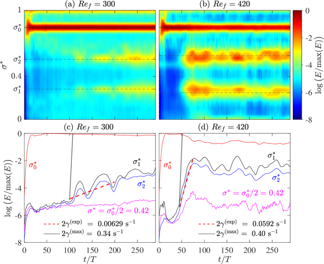
Figure 8: (a-b) Natural logarithm of the temporal energy spectra $E(\sigma,t,\Delta T)$ normalized by its maximum as a function of time $t$ and of the normalized frequency $\sigma^{*}=\sigma/2\Omega$ for the experiments at $Re_{f}=300$ (a) and $Re_{f}=420$ (b), computed using a sliding time window of $\Delta T=15\,T$. (c-d) Corresponding time evolution of the temporal energy spectra $E(\sigma,t,\Delta T)$ normalized by its maximum for four specific frequencies, $\sigma_{0}^{*}=0.84$, $\sigma_{1}^{*}$, $\sigma_{2}^{*}$ (reported in Table 1) and $\sigma^{*}=\sigma_{0}^{*}/2$, for the experiments at $Re_{f}=300$ (c) and $Re_{f}=420$ (d).

Before, it is important to uncover the time evolution of the flow from the start of the forcing. For this study, we focus on the region where the instability takes place (dashed rectangle in Fig. 7). We report in the top panels of Fig. 8 the natural logarithm of the temporal energy spectrum $E(\sigma,t,\Delta T)$ normalized by its maximum as a function of time $t$ and of the normalized frequency $\sigma^{*}=\sigma/2\Omega$ for the experiments at $Re_{f}=300$ and $Re_{f}=420$. These time-frequency spectra are computed using a short sliding time window of $\Delta T=15\,T$ in order to preserve the time resolution as much as possible while accessing a reasonably fine frequency resolution (although coarse obviously). In Fig. 8(a), for the experiment at $Re_{f}=300$, the subharmonic energy bumps start to be detectable after typically 100 forcing periods $T$. The amplitude of the subharmonic bumps then appear to slowly grow during the rest of the experiment. To have a more quantitative view, we report in Fig. 8(c) the time evolution of the energy density $E(\sigma,t,\Delta T)$ for four specific frequencies: the forcing frequency $\sigma_{0}^{*}=0.84$, the subharmonic frequencies $\sigma_{1}^{*}$ and $\sigma_{2}^{*}$ (reported in Table 1) and the frequency $\sigma^{*}=\sigma_{0}^{*}/2$ which is shown as a tracer of the spectral noise level (see Fig. 6). In Fig. 8(c), we observe that the initial increase of the amplitude of the primary wave typically takes $15$ forcing periods $T$. Using the theoretical value of the group velocity $|{\bf c_{g}}|=2\Omega\sin\theta/k_{0}\simeq 2.47$ cm/s of the primary wave, we can estimate the duration of the initial propagation of the primary wave through the studied region of $10\times 12$ cm² area to be of about $2$ to $3$ forcing periods $T$. The apparent duration of $15\,T$ of the growth in amplitude of the forced wave in Fig. 8(c) results from the time width of the sliding window used for the computation of the time-frequency spectra: processes taking place over a duration much shorter than $\Delta T$ have their duration artificially increased up to typically $\Delta T=15\,T$. This artificial spreading in time also explains the fact that we already observe the growth of the amplitude of the primary wave at $t=0$ while it is expected to start only after about $6\,T$ after the start of the forcing (the dashed rectangle is at a distance of about $30$ cm from the wave maker).

In Fig. 8(c), the amplitudes of the two subharmonic waves, which have a similar behavior, emerge from the spectral noise level around $t=100\,T$ after the start of the forcing, before they slowly grow until the end of the experiment at $t=300\,T$. By fitting the increase with time of the amplitude of the subharmonic bumps with the exponential behavior $E\sim\exp(2\gamma^{\rm(exp)}t)$ over the time period $100\,T<t<200\,T$, we estimate an experimental growth rate (for the velocity) of the subharmonic modes of $\gamma^{\rm(exp)}\simeq 3.1\,10^{-3}$ s^-1. This value is about fifty times smaller than the theoretical growth rate, of about $\gamma^{\rm(max)}\simeq 0.17$ s^-1, computed in the theoretical section II for a primary wave with features matching those of the experiment at $Re_{f}=300$ (details will be given in section IV.2 regarding this point). This discrepancy most probably reveals that the exponential growth of the subharmonic waves predicted at the onset of the TRI is restricted to earlier times in the experiment, before $t<100\,T$, for which unfortunately the subharmonic waves amplitude is too weak to be resolved by the PIV measurements. A natural interpretation for the low growth rate observed here for the subharmonic modes over the time period $100\,T<t<200\,T$ is that the saturation processes are already in action even if the saturation is not yet completed. Also, it is worth to note that we do not observe a significant broadening of the subharmonic bumps during their observable growth phase. This implies that the spreading in frequency of the subharmonic modes produced by the TRI does not necessarily result from the saturation processes of the instability.

For the experiment at $Re_{f}=420$ reported in Figs. 8(b) and (d), the scenario of the instability takes place much faster: the subharmonic bumps become detectable beyond $t\simeq 45\,T$ and then saturate in amplitude around $t\simeq 75\,T$. The experimental growth rate for the velocity amplitude of the modes at $\sigma_{1}^{*}$ and $\sigma_{2}^{*}$ during the period $45\,T<t<75\,T$ is here of about $\gamma^{\rm(exp)}\simeq 0.030$ s^-1. This value, much larger than the one measured for the experiment at $Re_{f}=300$, is still significantly smaller (seven times smaller) than the maximum theoretical growth rate, of about $\gamma^{\rm(max)}\simeq 0.20$ s^-1, that can be computed theoretically for a primary wave with features matching the ones of the experiment at $Re_{f}=420$. The observable growth of the subharmonic modes proceeds over a relatively short duration of about $30\,T$, of the same order as the width of the sliding window used to compute the spectra. Contrary to the experiment at $Re_{f}=300$, it is therefore here most likely that the measured growth rate is significantly biased (reduced) by the temporal spectrum computation and it is possible that the actual growth rate is not that far from the theoretical one. A final remark worth to be done regarding Fig. 8 is the fact that the forced wave, after its initial propagation through the studied area, experiences a slow decrease in amplitude during the stage where the secondary waves are increasing in amplitude, before finally reaching a stable state when the secondary waves saturate.

IV.2 Comparison of the experimental data to the theory

In this section, we focus on the region of the flow where the instability develops (the dashed rectangle in Fig. 7), where the three waves at $\sigma_{0}^{*}$, $\sigma_{1}^{*}$ and $\sigma_{2}^{*}$ are all energetic. We measure for each subharmonic mode the wavevector components in the measurement plane, $k_{x,i}^{\rm exp}$ and $k_{z,i}^{\rm exp}$, by spatially averaging the phase field gradient $\nabla\varphi$ over that region (the dashed rectangle). The corresponding measurement errors are computed as the standard deviation of the phase field gradient $\nabla\varphi$ over the same area.

Considering the observations of the previous section, the subharmonic waves are propagating out of the measurement plane ($x,z$) and should therefore have a non-zero wavevector component along the $y$-direction. We estimate this component by means of the dispersion relation of inertial waves (2) as

$$k_{y,i}^{\rm exp}=\pm\sqrt{\left(k_{z,i}^{\rm exp}\right)^{2}\left(\frac{1}{{\sigma_{i}^{*}}^{2}}-1\right)-\left(k_{x,i}^{\rm exp}\right)^{2}}\,.$$ (21)

For the secondary waves, we estimate $k_{y,i}^{\rm exp}$ by spatially averaging (21) over the instability region (the dashed rectangle in Fig. 7). We compute the corresponding error as the standard deviation of (21) over the same region. As a test, we apply this procedure to the primary wave of the experiment at $Re_{f}=300$ which leads to a negligible out-of-plane wavevector component $|k_{y,0}^{\rm exp}|=0.017$ rad/cm (computed as the root of the spatial mean of $|{k_{y,0}^{\rm exp}}|^{2}$ over the instability region) and a wavenumber $k_{0}^{\rm exp}=0.83\pm 0.02$ rad/cm in excellent agreement with the expected value $2\pi/(7.6$ cm$)\simeq 0.83$ rad/cm. The computed values of the wavevector components for the waves at $\sigma_{1}^{*}$ and $\sigma_{2}^{*}$ with the corresponding errors are reported in Table 1 for the experiments at $Re_{f}=300$ and $Re_{f}=420$, for which the TRI is observed.

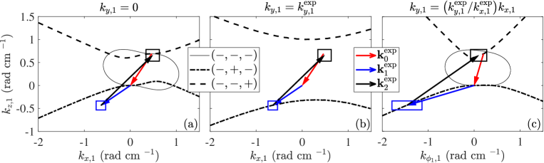
Figure 9: Cuts of the theoretical resonance surfaces for ${\bf k_{1}}$ computed for a primary wave of frequency $\sigma_{0}^{*}=0.84$, wavelength $\lambda_{f}=7.6\leavevmode\nobreak\$cm and amplitude $b_{0}=3.9$ mm/s matching the features of the experimental primary wave at $Re_{f}=300$ in its unstable region (dashed rectangle in Fig. 7). Superimposed on the resonance curves, we show the projection on the considered plane of the wavevectors ${\bf k_{0}^{\rm exp}}$, ${\bf k_{1}^{\rm exp}}$ and ${\bf k_{2}^{\rm exp}}$ experimentally estimated for the experiment at $Re_{f}=300$. We also report the measurement error corresponding to each wavevector component via a rectangle around each wavevector tip. (a) Cut in the vertical plane $k_{y,1}=0$. (b) Cut in the vertical plane $k_{y,1}=k_{y,1}^{\rm exp}$. (c) Cut in the vertical plane $k_{y,1}/k_{y,1}^{\rm exp}=k_{x,1}/k_{x,1}^{\rm exp}$ ($k_{\phi_{1},1}=\sqrt{k_{x,1}^{2}+k_{y,1}^{2}}=k_{x,1}\sqrt{1+(k_{y,1}^{\rm exp}/k_{x,1}^{\rm exp})^{2}}).$

In Fig. 9, we report three different cuts of the resonance surfaces for ${\bf k_{1}}$ computed theoretically for a primary wave of frequency $\sigma_{0}^{*}=0.84$, wavelength $\lambda_{f}=7.6\leavevmode\nobreak\$cm, and amplitude $b_{0}=3.9$ mm/s. These values match the features of the experimental primary wave at $Re_{f}=300$ in its unstable region (dashed rectangle in Fig. 7). For each cutting plane, the resulting curves for the three possible polarities combinations are shown. In panel (a), we report the classical resonance curves for ${\bf k_{1}}$ in the plane ($k_{x},k_{z}$) of the primary wave ($k_{y,1}=0$). We superimpose on this figure the projections of the experimentally computed wavevectors ${\bf k_{1}^{\rm exp}}$ and ${\bf k_{2}^{\rm exp}}$ and of the primary wavevector ${\bf k_{0}^{\rm exp}}$ on the ($k_{x},k_{z}$) plane. We also report the measurement error of each wavevector component via a rectangle around each wavevector tip. We recall that the frequencies $\sigma_{1}$ and $\sigma_{2}$ are predicted negative by the theory (see Sec. II). In parallel, they are definite positive in the experimental data processing. In order to compare the experimental data to the theory, in the following, we therefore systematically multiply by $-1$ the experimentally measured wavevectors ${\bf k_{1}^{\rm exp}}$ and ${\bf k_{2}^{\rm exp}}$ before superimposing them on the theoretical curves, starting with Fig. 9 [note that waves with ($\sigma,{\bf k}$) and ($-\sigma,-{\bf k}$) are the same]. In Fig. 9(a), we observe that the three wavevectors form an almost closed triangle in the vertical plane ($k_{x},k_{z}$), i.e., $\mathbf{k}_{0}^{\rm exp}+\mathbf{k}_{1}^{\rm exp}+\mathbf{k}_{2}^{\rm exp}\simeq{\bf 0}$: this confirms the spatial resonance of the three waves involved in the instability, at least in the vertical plane ($k_{x},k_{z}$). Nevertheless, it is clear that the tip of the experimentally measured wavevector $(k_{x,1}^{\rm exp},k_{z,1}^{\rm exp})$ does not fall on one of the ${\bf k_{1}}$ resonance curves of the in-plane triadic resonance instability. In panel (b), we show the theoretical resonance curves for ${\bf k_{1}}$ in the plane $k_{y,1}=k_{y,1}^{\rm exp}$ on which we again superimpose the projection of the experimentally measured wavevectors ${\bf k_{0}^{\rm exp}}$, ${\bf k_{1}^{\rm exp}}$ and ${\bf k_{2}^{\rm exp}}$ on the ($k_{x},k_{z}$) plane. This time the nearly closed wavevectors triad has its ${\bf k_{1}^{\rm exp}}$ tip almost exactly on the ($-,+,-$) resonance curve. In the last panel (c), we show the theoretical ${\bf k_{1}}$ resonance curves in the plane $k_{y,1}/k_{y,1}^{\rm exp}=k_{x,1}/k_{x,1}^{\rm exp}$. In this plane, the projection of the experimental wavevectors triad is again almost closed and its ${\bf k_{1}}$ tip lies almost exactly on the ($-,+,-$) resonance curve. Altogether Fig. 9 confirms, in agreement with the theoretical arguments of Sec. II, the experimental observation of a three-dimensional triadic resonance instability of type ($-,+,-$) driving the primary wave energy toward two subharmonic waves not propagating in the same vertical plane as the primary wave.

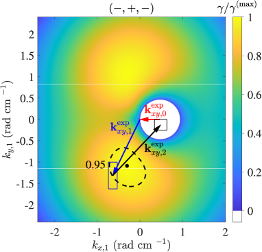
Figure 10: Map of the growth rate $\gamma$ normalized by its maximum $\gamma^{\rm(max)}$ as a function of $(k_{x,1},k_{y,1})$ for the ($-,+,-$) instability computed theoretically for a primary wave with features [$\sigma_{0}^{*}=0.84$, $\lambda_{f}=7.6\leavevmode\nobreak\$cm, $b_{0}=3.9$ mm/s] matching the experimental primary wave at $Re_{f}=300$ (same map as in Fig. 2). Superimposed on the $\gamma/\gamma^{\rm(max)}$ map, we show the projection in the $(k_{x},k_{y})$ plane of the experimental wavevectors ${\bf k_{0}^{\rm exp}}$, ${\bf k_{1}^{\rm exp}}$ and ${\bf k_{2}^{\rm exp}}$. As in Fig. 9, the measurement errors on the wavevectors are reported via a rectangle around each wavevector tip.

To further compare the experimental data with the theoretical predictions, we report in Fig. 10 the map of the growth rate $\gamma$ as a function of $(k_{x,1},k_{y,1})$ for the ($-,+,-$) instability. This map is computed for a primary wave with features [$\sigma_{0}^{*}=0.84$, $\lambda_{f}=7.6\leavevmode\nobreak\$cm, $b_{0}=3.9$ mm/s] matching the experimental primary wave characteristics at $Re_{f}=300$ (same parameters as in Fig. 2). We superimpose to the map of $\gamma$ the projection on the $(k_{x},k_{y})$ plane of the experimental wavevectors ${\bf k_{0}^{\rm exp}}$, ${\bf k_{1}^{\rm exp}}$ and ${\bf k_{2}^{\rm exp}}$ at $Re_{f}=300$. First, we observe that the experimental triad in the ($k_{x},k_{y}$) plane is also close to spatial resonance with the wavevectors tending to form a closed triangle. Moreover, the tip of the ${\bf k_{1}^{\rm exp}}$ wavevector is near the location of the maximum of the theoretical instability growth rate: it is included in the region where $\gamma$ is larger than $95\%$ of its maximum. The latter observation shows that the features of the triadic resonance instability observed in the experiment at $Re_{f}=300$ are consistent with the theoretical predictions based on the selection of the maximum growth rate.

We recall here that the theory presented in Sec. II focuses on the early times of the instability during which the amplitudes of the subharmonic secondary waves grow exponentially from low values. In parallel, as already discussed, we are not able to study experimentally the initial exponential growth of the subharmonic waves because during this stage the subharmonic waves amplitude is smaller than the resolution of our PIV measurements. Therefore, the experimental characterization of the subharmonic waves is conducted over the whole experiment duration. The growing influence of the saturation processes observed during the experiment at $Re_{f}=300$ can possibly lead to discrepancies between the maximum growth rate modes expected to be dominant at the early stages of the instability and the dominant modes present in the experimentally studied stage where the subharmonic waves are detectable. It is therefore even more remarkable to observe such an excellent agreement between the theoretical predictions of the 3D TRI at early times and our measurements. Finally, recalling that the map of the theoretical growth rate $\gamma(k_{x,1},k_{y,1})$ is symmetric with respect to the $k_{y,1}=0$ axis with two symmetric maxima, we should mention that in Fig. 10 when computing $k_{y,1}^{\rm exp}$ from Eq. (21), we arbitrarily choose the sign of the $y$ wavevector component, the most probable situation being that both signs are present in reality. Another remark is worth to be done: References Bourget2014 and Karimi2014 have shown that refinements to the model of the triadic resonance instability can be done in order to account for the finite size of the wave beam, i.e., for the finite number of wavelengths contained in the beam width. In Appendix B, we show that, after including to the theory the finite size corrections proposed by Bourget et al. Bourget2014 , the map of the theoretical growth rate is only slightly modified by the finite size effects and that the good agreement between the experimental triad and the most unstable theoretical triad is preserved.

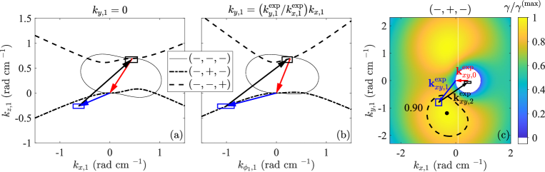
Figure 11: (a-b) Cuts of the theoretical resonance surfaces for ${\bf k_{1}}$ computed for a primary wave of frequency $\sigma_{0}^{*}=0.84$, wavelength $\lambda_{f}=7.6\leavevmode\nobreak\$cm and amplitude $b_{0}=5.1$ mm/s matching the features of the experimental primary wave at $Re_{f}=420$. Superimposed on the resonance curves, we show the projection on the considered plane of the wavevectors ${\bf k_{0}^{\rm exp}}$, ${\bf k_{1}^{\rm exp}}$ and ${\bf k_{2}^{\rm exp}}$ measured for the experiment at $Re_{f}=420$. (a) Cut in the vertical plane $k_{y,1}=0$. (b) Cut in the vertical plane $k_{y,1}/k_{y,1}^{\rm exp}=k_{x,1}/k_{x,1}^{\rm exp}$. (c) Map of the growth rate $\gamma$ normalized by its maximum $\gamma^{\rm(max)}$ as a function of $(k_{x,1},k_{y,1})$ for the ($-,+,-$) instability computed theoretically for a primary wave matching the features of the experimental primary wave at $Re_{f}=420$. Superimposed on the $\gamma/\gamma^{\rm(max)}$ map, we show the projection in the $(k_{x},k_{y})$ plane of the experimental wavevectors ${\bf k_{0}^{\rm exp}}$, ${\bf k_{1}^{\rm exp}}$ and ${\bf k_{2}^{\rm exp}}$.

In the following we reproduce the same analysis for the experiment at $Re_{f}=420$. In Fig. 11, we report the cut of the theoretical resonance surface for ${\bf k_{1}}$ in the planes $k_{y,1}=0$ (panel a) and $k_{y,1}/k_{y,1}^{\rm exp}=k_{x,1}/k_{x,1}^{\rm exp}$ (panel b) on which we superimpose the projection of the experimental wavevectors triad corresponding to the maximum of energy in the first subharmonic bump of the temporal energy spectrum (Fig. 6). In Fig. 11(c), we show the map of the theoretical growth rate $\gamma$ as a function of $(k_{x,1},k_{y,1})$ for the ($-,+,-$) instability. This map is computed for a primary wave with features [$\sigma_{0}^{*}=0.84$, $\lambda_{f}=7.6\leavevmode\nobreak\$cm, $b_{0}=5.1$ mm/s] matching the experimental primary wave characteristics at $Re_{f}\simeq 420$. We also superimpose to the map of $\gamma$ the projection on the $(k_{x},k_{y})$ plane of the experimental wavevectors triad at $Re_{f}=420$. In all panels of Fig. 11, we verify the fact that the experimental triad is nearly closed confirming the spatial resonance of the temporally resonant waves. In panel (b), the tip of the ${\bf k_{1}}$ experimental wavevector again falls very well on the $(-,+,-)$ theoretical resonance curve whereas it is at a significant distance from the 2D resonance curve in the $k_{y,1}=0$ plane (panel a). Finally, in panel (c), we observe that the tip of the ${\bf k_{1}}$ experimental wavevector is significantly remote from the maximum of the growth rate map. It is however found within the region where the theoretical growth rate $\gamma$ is larger than $90\%$ of its maximum which is rather satisfactory considering that, for this experiment at $Re_{f}=420$, the analysis is dominated by the saturated regime of the TRI which is not the case for the previously studied experiment at $Re_{f}=300$ which is closer to the instability onset.

V Conclusion

In this article, we report PIV measurements of the velocity field produced in a rotating fluid by a wave generator. The wave maker is designed to produce a wave beam approaching the structure of a plane inertial wave. In practice, the wave beam contains four wavelengths in its width. Besides, the wave generator is particularly large in the horizontal direction $y$ in which the plane wave is supposed to be invariant: the generator extension in the $y$-direction corresponds to nearly seven wavelengths. This last feature is radically different from previous experiments aiming to produce plane inertial (or internal gravity) waves where the wave maker extension in the $y$-direction was (slightly) smaller than two wavelengths Bordes2012 ; Joubaud2012 ; Bourget2013 ; Bourget2014 . Starting from the linear regime, we increase the forcing amplitude in order to explore the emergence of the non-linear effects affecting the forced inertial wave. Above a given threshold in amplitude, the forced wave is subject to an instability transferring some of its energy toward two subharmonic inertial waves in temporal and spatial triadic resonance with the primary wave. We nevertheless show that the secondary waves are not propagating in the same vertical plane as the primary wave: they are non-invariant in the horizontal direction $y$ along which the primary wave is invariant. This spontaneous breaking of the symmetry of the base flow shows that the triadic resonance instability of the forced inertial wave is three-dimensional.

In parallel, by building on the classical inertial wave triadic interaction coefficients, we compute numerically the growth rate of the triadic resonance instability (TRI) of a plane inertial wave in the three-dimensional case. We show that the maximum growth rate is associated with a three-dimensional instability producing two secondary waves propagating out of the primary wave vertical plane. We also show that this result can be demonstrated analytically in the inviscid case where the TRI becomes a Parametric Subharmonic Instability (PSI) Staquet2002 ; Dauxois2018 with two secondary waves at vanishing scale and at frequencies equal to half the primary wave frequency. Finally, we demonstrate that the secondary wavevectors observed in our experiments agree well with the triad predicted theoretically by the maximization of the theoretical instability growth rate. This agreement with the theory for a plane wave confirms that the three-dimensionality of the TRI observed experimentally is intrinsic and unrelated to deviations of the experimental primary wave from an exact plane wave (due to friction on the water tank walls, finite size effects …).

An important consequence of our results concerns flows in the wave turbulence regime (at larger Reynolds number than the ones considered here) Monsalve2020 ; LeReun2021 . One of the key assumptions made when deriving the scaling laws for the spatial energy spectrum from the kinetic equations in weak inertial-wave turbulence theory Galtier2003 is the statistical axisymmetry of the flow around the rotation axis. We have shown in the present article that the triadic resonant interactions between inertial waves are very efficient at redistributing the energy in the horizontal plane, normal to rotation. This feature should contribute to drive flows in the inertial wave turbulence regime toward statistical axisymmetry and to make them fulfill the assumption made in the derivation of the wave turbulence theory Galtier2003 .

At this point, an interesting question concerns the triadic resonance instability of an internal gravity wave: is it two or three-dimensional ? In the 2D case (invariant in horizontal direction $y$), the expression of the triadic interaction coefficients and of the growth rate of the TRI for internal gravity waves are analogous to those for inertial waves Maurer2016 . However, this similarity seems not to hold when considering 3D triadic interactions of waves propagating in different vertical planes Remmel2014 and only a dedicated study will provide answers in the case of internal gravity waves. The question of the three-dimensionality of the TRI for an internal gravity wave has been recently tackled by Ghaemsaidi and Mathur Ghaemsaidi2019 who implemented a local stability analysis for a plane internal gravity wave. Their analysis, restricted to the inviscid limit and to small scale perturbations —i.e., the Parametric Subharmonic Instability case— shows that a three-dimensional PSI is possible for an internal gravity wave. However, the instability associated with the maximum growth rate is shown to remain two-dimensional with secondary waves propagating in the same vertical plane as the primary wave. The local stability analysis of Ghaemsaidi and Mathur predicts that the internal wave instability starts to be dominated by three-dimensional processes when the primary wave becomes strongly non-linear, i.e. with a Froude number (equivalent to the Rossby number in stratified fluids) larger than $1$. In this situation, the instability growth rate is shown to be larger than the internal wave frequencies: the flow is completely out of the weakly non-linear framework of the triadic resonance instability.

The three-dimensionality of the TRI of an internal gravity wave toward two subharmonic waves of finite wavelengths remains an open question, to be investigated theoretically and experimentally. More generally, the question of the energy redistribution in the horizontal plane normal to gravity by internal gravity wave triadic interactions remains open with important stakes regarding the conditions under which the wave turbulence formalism for stratified fluids Caillol2000 ; Lvov2001 ; Lvov2004 could be relevant.

Appendix A Asymptotic expression of the growth rate in the inviscid limit

Using Eq. (13), the growth rate of the triadic resonance instability of a plane inertial wave is given by

$$\gamma=\frac{-\nu(k_{1}^{2}+k_{2}^{2})}{2}+\sqrt{\frac{\nu^{2}(k_{1}^{2}-k_{2}^{2})^{2}}{4}+C_{1}\overline{C_{2}}|b_{0}|^{2}}\,,$$ (22)

where, according to Waleffe Waleffe1992 ,

$$C_{1}\overline{C_{2}}=\frac{\sin^{2}\alpha_{2}}{4k_{2}^{2}}\left(s_{0}k_{0}+s_{1}k_{1}+s_{2}k_{2}\right)^{2}\left(s_{0}k_{0}-s_{2}k_{2}\right)\left(s_{1}k_{1}-s_{0}k_{0}\right)\,.$$ (23)

Following Eq. (8) of Smith and Waleffe Smith1999 (which is the direct consequence of the dispersion relation combined to the triadic resonance conditions (9-10)), one can show that

$$\left(s_{0}k_{0}-s_{2}k_{2}\right)=\frac{\sigma_{1}}{\sigma_{0}}\left(s_{2}k_{2}-s_{1}k_{1}\right)\quad{\rm and}\quad\left(s_{0}k_{0}-s_{1}k_{1}\right)=\frac{\sigma_{2}}{\sigma_{0}}\left(s_{1}k_{1}-s_{2}k_{2}\right)\,,$$ (24)

such that

$$C_{1}\overline{C_{2}}=\frac{\sin^{2}\alpha_{2}}{4k_{2}^{2}}\left(s_{0}k_{0}+s_{1}k_{1}+s_{2}k_{2}\right)^{2}\frac{\sigma_{1}\sigma_{2}}{\sigma_{0}^{2}}\left(s_{1}k_{1}-s_{2}k_{2}\right)^{2}\,.$$ (25)

In the following, we conduct an asymptotic expansion of the inviscid growth rate $\gamma=|b_{0}|\sqrt{C_{1}\overline{C_{2}}}$ to the first order in $k_{0}/k_{1}\simeq k_{0}/k_{2}$ assuming that the secondary wavenumbers associated to the maximum growth rate are much larger than the primary wavenumber such that $|\sigma_{1}|=|\sigma_{2}|=\sigma_{0}/2$ and $k_{1}\simeq k_{2}\gg k_{0}$. Focusing on the combination of wave polarities $(s_{0}=-1,s_{1}=+1,s_{2}=-1)$, the growth rate can be written

$$\gamma \simeq \frac{|b_{0}|}{4k_{2}}\sin\alpha_{2}\sqrt{\left(k_{0}-k_{1}+k_{2}\right)^{2}\left(k_{2}+k_{1}\right)^{2}}\,,$$ (26)

$$\simeq \frac{|b_{0}|}{4k_{2}}\sin\alpha_{2}\sqrt{\left(k_{0}(k_{1}+k_{2})+k_{2}^{2}-k_{1}^{2}\right)^{2}}\,.$$ (27)

Using the law of cosines

$$\cos\alpha_{2}=\frac{k_{0}^{2}+k_{1}^{2}-k_{2}^{2}}{2k_{1}k_{0}},$$ (28)

Eq. (27) gives, to the first order in $k_{0}/k_{1}\simeq k_{0}/k_{2}$,

$$\frac{\gamma}{|b_{0}|k_{0}} \simeq \frac{1}{2}\sin\alpha_{2}(1-\cos\alpha_{2})\,.$$ (29)

Maximizing equation (29) with respect to $\alpha_{2}$ yields

$$\cos\alpha_{2}=-1/2$$ (30)

corresponding to an angle $\alpha_{2}=2\pi/3$ rad ($=120^{\circ}$) and to a growth rate equal to

$$\gamma^{\rm(max)}\simeq 0.6495\,|b_{0}|k_{0}.$$ (31)

Injecting this specific value $\alpha_{2}=2\pi/3$ rad in the law (28), one gets

$$k_{2}^{2}=k_{1}^{2}+k_{0}^{2}+k_{0}k_{1}\,.$$ (32)

Retaining the sign conventions used in Sec. II, the primary wave vector can be written ${\bf k_{0}}=(k_{x,0},0,k_{z,0})=(-k_{0}\sin\theta_{0},0,-k_{0}\cos\theta_{0})$ with $\theta_{0}=\cos^{-1}(\sigma_{0}^{*})$. Besides, we note ${\bf k_{1}}=(k_{x,1},k_{y,1},k_{z,1})=(-k_{1}\sin\theta_{1}\cos\phi_{1},-k_{1}\sin\theta_{1}\sin\phi_{1},-k_{1}\cos\theta_{1})$ the components of the wave vector of secondary wave $1$ with $\theta_{1}=\cos^{-1}(|\sigma_{1}^{*}|)$. Using the spatial resonance condition

$$k_{2}^{2}=(k_{x,1}+k_{x,0})^{2}+k_{y,1}^{2}+(k_{z,1}+k_{z,0})^{2}\,,$$ (33)

one gets

$$k_{0}\,k_{1} = 2\,{\bf k_{0}}\cdot{\bf k_{1}}\,,$$ (34)

$$= k_{0}\,k_{1}\left(2\sin\theta_{0}\sin\theta_{1}\cos\phi_{1}+2\cos\theta_{0}\cos\theta_{1}\right)\,.$$ (35)

Using now the fact that the secondary wave $1$ maximizing the growth rate verifies $|\sigma_{1}^{*}|=\cos\theta_{1}=\sigma_{0}^{*}/2=\cos\theta_{0}/2$ in the inviscid limit, we obtain

$$\sin\theta_{0}=2\sin\theta_{1}\cos\phi_{1}\,,$$ (36)

which finally leads to

$$\cos^{2}\phi_{1}=\frac{1-{\sigma^{*}_{0}}^{2}}{4-{\sigma^{*}_{0}}^{2}}\,,$$ (37)

and to

$$\frac{k_{y,1}}{k_{x,1}}=\tan\phi_{1}=\pm\sqrt{\frac{3}{1-{\sigma^{*}_{0}}^{2}}}\,.$$ (38)

Appendix B Accounting for finite size effects

In Ref. Bourget2014 , Bourget et al. propose a refined theoretical description of the triadic resonance instability of an internal gravity wave accounting for the finite size of the wave beam (see also Ref. Karimi2014 on this topic). They consider the instability of a monochromatic wave beam modulated in its transverse direction by a rectangular function of width $W$. Their description is based on an energy budget realized inside a control volume matching the beam width $W$ where the TRI takes place. In the following, we reproduce this model for an inertial wave and modify it accordingly: the viscous dissipation rate for an inertial wave of wavenumber $k$ is $\nu k^{2}$ Machicoane2018 whereas it is $\nu k^{2}/2$ for an internal gravity wave Sutherland2010 . Then, in the equations of evolution of the secondary wave amplitudes (Eqs. 11-12), the dissipation rate $\nu k_{i}^{2}$ for the secondary wave $i$ must be replaced by $\chi_{i}=\nu k_{i}^{2}+|{\bf c_{g,i}}\cdot{\bf{\hat{k}_{0}}}|/2W$ with ${\bf c_{g,i}}$ the group velocity of wave $i$ and $\bf{\hat{k}_{0}}$ the unit vector parallel to the primary wave vector. The additional term $|{\bf c_{g,i}}\cdot{\bf{\hat{k}_{0}}}|/2W$ actually accounts for the rate at which the energy of the secondary wave $i$ is leaving the control volume where the instability takes place. Finally, the TRI growth rate for an inertial wave beam of transverse width $W$ becomes

$$\gamma=-\frac{\chi_{1}+\chi_{2}}{2}+\sqrt{\frac{(\chi_{1}-\chi_{2})^{2}}{4}+{\color[rgb]{0,0,0}C_{1}\overline{C_{2}}}|b_{0}|^{2}}\,.$$ (39)

The contribution of the additional damping term $|{\bf c_{g,i}}\cdot{\bf{\hat{k}_{0}}}|/2W$ due to the beam finite size will reduce the growth rate and stabilize certain triads that were unstable for an “infinite” plane wave.

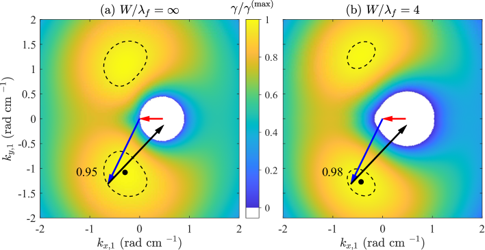
Figure 12: Map of the growth rate $\gamma$ normalized by its maximum $\gamma^{\rm(max)}$ as a function of $(k_{x,1},k_{y,1})$ for the ($-,+,-$) instability computed theoretically for a primary wave with features [$\sigma_{0}^{*}=0.84$, $\lambda_{f}=7.6\leavevmode\nobreak\$cm, $b_{0}=3.9$ mm/s] matching the experimental primary wave at $Re_{f}=300$. Superimposed on the $\gamma/\gamma^{\rm(max)}$ map, we show the projection in the $(k_{x},k_{y})$ plane of the wavevectors ${\bf k_{0}^{\rm exp}}$, ${\bf k_{1}^{\rm exp}}$ and ${\bf k_{2}^{\rm exp}}$ estimated experimentally. (a) Growth rate map for an (infinite) plane wave (same map as in Fig. 10). (b) Growth rate map for a wave beam with four wavelengths in its width $W=4\lambda_{f}$ following Eq. (39).

It is interesting to analyze to what extent including these finite size effects modifies the theoretical prediction for the most unstable triad, and its agreement with the experimental triad reported in the present article. Focusing on the primary wave parameters of the experiment at $Re_{f}=300$ (analyzed in Figs. 7-10), we report in Fig. 12 the map of the theoretical growth rate for a primary plane wave on the left and for a wave beam of width $W=4\lambda_{f}$ on the right, corresponding to the experimental wave beam containing four wavelengths in its width. As in Fig. 10, we superimpose on these maps the experimental wavevectors triad projected on the plane ($k_{x,1},k_{y,1}$) (Fig. 12(a) is identical to Fig. 10).

Overall, the map of the growth rate is only slightly modified by the finite size effects. For instance, in the plane ($k_{x,1},k_{y,1}$) the tip of the theoretical wavevector ${\bf k_{1}}$ associated with the maximum growth rate is shifted of a relative distance of $20\%$ (compared to the value of $\sqrt{k_{x,1}^{2}+k_{y,1}^{2}}$). Besides, there is a better agreement between the experimental wavevectors triad and the theoretical triad with the maximum growth rate: the tip of the experimental vector ${\bf k_{1}}$ is now included in the region where the theoretical growth rate is larger than $98\%$ of its maximum whereas it was $95\%$ when finite size effects where not accounted for. We realize that the conclusions put forward in the present article are not modified by the finite size of the primary wave beam: the refined model does still predict that the TRI is tridimensional and the agreement between the experimental TRI and the theory is conserved (and even slightly improved).

References

- (1) H.P. Greenspan, The Theory of Rotating Fluids (Cambridge University Press, Cambridge, UK, 1968).
- (2) J. Lighthill, Waves in Fluids (Cambridge University Press, Cambridge, UK, 1978).
- (3) B.R. Sutherland, Internal Gravity Waves (Cambridge University Press, Cambridge, UK, 2010).
- (4) M. Brunet, T. Dauxois, and P.-P. Cortet, Linear and non linear regimes of an inertial wave attractor, Phys. Rev. Fluids. 4, 034801 (2019).
- (5) D.E. Mowbray and B.S.H. Rarity, A theoretical and experimental investigation of the phase configuration of internal waves of small amplitude in a density stratified liquid, J. Fluid Mech. 28, 1 (1967).
- (6) N.H. Thomas and T.N. Stevenson, A similarity solution for viscous internal waves, J. Fluid Mech. 54, 495 (1972).
- (7) M. R. Flynn, K. Onu, and B. R. Sutherland, Internal wave excitation by a vertically oscillating sphere, J. Fluid Mech. 494, 65 (2003).
- (8) P.-P. Cortet, C. Lamriben, and F. Moisy, Viscous spreading of an inertial wave beam in a rotating fluid, Phys. Fluids 22, 086603 (2010).
- (9) N. Machicoane, P.-P. Cortet, B. Voisin, and F. Moisy, Influence of the multipole order of the source on the decay of an inertial wave beam in a rotating fluid, Phys. Fluids 27, 066602 (2015).
- (10) M. Mercier, D. Martinand, M. Mathur, L. Gostiaux, T. Peacock, and T. Dauxois, New wave generation, J. Fluid Mech. 657, 310 (2010).
- (11) G. Bordes, F. Moisy, T. Dauxois, and P.-P. Cortet, Experimental evidence of a triadic resonance of plane inertial waves in a rotating fluid, Phys. Fluids 24, 014105 (2012).
- (12) B. Bourget, T. Dauxois, S. Joubaud and P. Odier, Experimental study of parametric subharmonic instability for internal plane waves, J. Fluid Mech. 723, 1 (2013).
- (13) K.D. Aldridge and A. Toomre, Axisymmetric inertial oscillations of a fluid in a rotating spherical container, J. Fluid Mech. 37, 307 (1969).
- (14) A.D. McEwan, Inertial oscillations in a rotating fluid cylinder, J. Fluid Mech. 40, 603 (1970).
- (15) L.R.M. Maas, On the amphidromic structure of inertial waves in rectangular parallelepiped, Fluid Dyn. Res. 33, 373 (2003).
- (16) J. Boisson, C. Lamriben, L.R.M. Maas, P.-P. Cortet, and F. Moisy, Inertial waves and modes excited by the libration of a rotating cube, Phys. Fluids 24, 076602 (2012).
- (17) J. Boisson, D. Cébron, F. Moisy, and P.-P. Cortet, Earth rotation prevents exact solid-body rotation of fluids in the laboratory, EPL 98, 59002 (2012).
- (18) L.R.M. Maas, D. Benielli, J. Sommeria, and F.-P. A. Lam, Observation of an internal wave attractor in a confined, stably stratified fluid, Nature 388, 557 (1997).
- (19) M. Rieutord, B. Georgeot, and L. Valdettaro, Inertial waves in a rotating spherical shell: attractors and asymptotic spectrum, J. Fluid Mech. 435, 103 (2001).
- (20) A.M.M. Manders and L.R.M. Maas, Observations of inertial waves in a rectangular basin with one sloping boundary, J. Fluid Mech. 493, 39 (2003).
- (21) N. Grisouard, C. Staquet, and I. Pairaud, Numerical simulation of a two-dimensional internal wave attractor, J. Fluid Mech. 614, 1 (2008).
- (22) M. Klein, T. Seelig, M.V. Kurgansky, A. Ghasemi, I.D. Borcia, A. Will, E. Schaller, C. Egbers and U. Harlander, Inertial wave excitation and focusing in a liquid bounded by a frustum and a cylinder, J. Fluid Mech. 751, 255 (2014).
- (23) J. Pedlosky, Geophysical Fluid Dynamics (Springer-Verlag, New York, 1987).
- (24) V.E. Zakharov, V.S. L’vov, and G. Falkovich, Kolmogorov Spectra of Turbulence (Springer, Berlin, 1992).
- (25) A.C. Newell and B. Rumpf, Wave Turbulence, Annu. Rev. Fluid Mech. 43, 59 (2011).
- (26) S. Nazarenko, Wave Turbulence (Springer, Berlin, 2011).
- (27) M.C. Gregg, E.A. D’Asaro, J.J. Riley, and E. Kunze, Mixing efficiency in the ocean, Ann. Rev. Mar. Sci. 10, 443 (2018).
- (28) E. Monsalve, M. Brunet, B. Gallet, P.-P. Cortet, Quantitative Experimental Observation of Weak Inertial-Wave Turbulence, Phys. Rev. Lett. 125, 254502 (2020).
- (29) N. Yokoyama and M. Takaoka, Energy-flux vector in anisotropic turbulence: Application to rotating turbulence, J. Fluid Mech. 908, A17 (2021).
- (30) T. Le Reun, B. Favier, and M. Le Bar, Evidence of the Zakharov-Kolmogorov spectrum in numerical simulations of inertial wave turbulence, Europhys. Lett. 132, 64002 (2020).
- (31) C. Savaro, A. Campagne, M. Calpe Linares, P. Augier, J. Sommeria, T. Valran, S. Viboud, and N. Mordant, Generation of weakly nonlinear turbulence of internal gravity waves in the Coriolis facility, Phys. Rev. Fluids 5, 073801 (2020).
- (32) G. Davis, T. Jamin, J. Deleuze, S. Joubaud, and T. Dauxois, Succession of Resonances to Achieve Internal Wave Turbulence, Phys. Rev. Lett. 124, 204502 (2020).
- (33) S. Galtier, Weak inertial-wave turbulence theory, Phys. Rev. E 68, 015301 (2003).
- (34) C. Cambon, R. Rubinstein, and F.S. Godeferd, Advances in wave turbulence: rapidly rotating flows, New J. Phys. 6, 73 (2004).
- (35) Y.V. Lvov, K.L. Polzin, and E.G. Tabak, Energy Spectra of the Ocean’s Internal Wave Field: Theory and Observations, Phys. Rev. Lett. 92, 128501 (2004).
- (36) S.V. Nazarenko and A.A. Schekochihin, Critical balance in magnetohydrodynamic, rotating and stratified turbulence: towards a universal scaling conjecture, J. Fluid Mech. 677, 134 (2011).
- (37) L.M. Smith and F. Waleffe, Transfer of energy to two-dimensional large scales in forced, rotating three-dimensional turbulence, Phys. Fluids 11, 1608 (1999).
- (38) C. Staquet and J. Sommeria, Internal gravity waves: From instabilities to turbulence, Annu. Rev. Fluid Mech. 34, 559 (2002).
- (39) C. R. Koudella and C. Staquet, Instability mechanisms of a two-dimensional progressive internal gravity wave, J. Fluid Mech. 548, 165 (2006).
- (40) S. Joubaud, J. Munroe, P. Odier, and T. Dauxois, Experimental parametric subharmonic instability in stratified fluids, Phys. Fluids 24, 041703 (2012).
- (41) B. Bourget, H. Scolan, T. Dauxois, M. Le Bars, P. Odier, and S. Joubaud, Finite-size effects in parametric subharmonic instability, J. Fluid Mech. 759, 739 (2014).
- (42) L. Jouve and G. I. Ogilvie, Direct numerical simulations of an inertial wave attractor in linear and nonlinear regimes, J. Fluid Mech. 745, 223 (2014).
- (43) H. Scolan, E. Ermanyuk, and T. Dauxois, Nonlinear fate of internal waves attractors, Phys. Rev. Letters 110, 234501 (2013).
- (44) C. Brouzet, E. Ermanyuk, S. Joubaud, G. Pillet, and T. Dauxois, Internal wave attractors: different scenarios of instability, J. Fluid Mech. 811, 544 (2017).
- (45) H.H. Karimi and T.R. Akylas, Parametric subharmonic instability of internal waves: Locally confined beams versus monochromatic wave trains, J. Fluid Mech. 757, 381 (2014).
- (46) N. Machicoane, V. Labarre, B. Voisin, F. Moisy, and P.-P. Cortet, Wake of inertial waves of a horizontal cylinder in horizontal translation, Phys. Rev. Fluids 3, 034801 (2018).
- (47) M.J. Lighthill, On waves generated in dispersive systems by travelling forcing effects, with applications to the dynamics of rotating fluids, J. Fluid Mech. 27, 725 (1967).
- (48) T. Le Reun, B. Gallet, B. Favier, and M. Le Bars, Near-resonant instability of geostrophic modes: beyond Greenspan’s theorem, J. Fluid Mech. 900, R2 (2020).
- (49) M. Brunet, B. Gallet, and P.-P. Cortet, Shortcut to Geostrophy in Wave-Driven Rotating Turbulence: The Quartetic Instability, Phys. Rev. Lett. 124, 124501 (2020).
- (50) A.D.D. Craik and J.A. Adam, Evolution in space and time of resonant wave triads-I. The ‘pump-wave approximation’, Proc. R. Soc. Lond. A. 363, 243 (1978).
- (51) S. Gururaj and A. Guha, Energy transfer in resonant and near-resonant internal wave triads for weakly non-uniform stratifications. Part 1. Unbounded domain, J. Fluid Mech. 899, A6 (2020).
- (52) F. Waleffe, The nature of triad interactions in homogeneous turbulence, Phys. Fluids A 4, 350 (1992).
- (53) F. Waleffe, Inertial transfers in the helical decomposition, Phys. Fluids A 5, 677 (1993).
- (54) S.A. Triana, D.S. Zimmerman, and D.P. Lathrop, Precessional states in a laboratory model of the Earth’s core, J. Geophys. Res. 117, B04103 (2012).
- (55) T. Le Reun, B. Favier, and M. Le Bars, Experimental study of the nonlinear saturation of the elliptical instability: inertial wave turbulence versus geostrophic turbulence, J. Fluid Mech. 879, 296 (2019).
- (56) M.J. Mercier, N.B. Garnier, and T. Dauxois, Reflection and diffraction of internal waves analyzed with the Hilbert transform, Phys. Fluids 20, 086601 (2008).
- (57) T. Dauxois, S. Joubaud, P. Odier, and A. Venaille, Instabilities of Internal Gravity Wave Beams, Annu. Rev. Fluid Mech. 50, 131 (2018).
- (58) P. Maurer, S. Joubaud, and P. Odier, Generation and stability of inertial gravity waves, J. Fluid Mech. 808, 539 (2016).
- (59) M. Remmel, J. Sukhatme, and L.M. Smith, Nonlinear gravity-wave interactions in stratified turbulence, Theor. Comput. Fluid Dyn. 28, 131 (2014).
- (60) S. Ghaemsaidi and M. Mathur, Three-dimensional small-scale instabilities of plane internal gravity waves, J. Fluid Mech. 863, 702 (2019).
- (61) Y.V. Lvov and E.G. Tabak, Hamiltonian Formalism and the Garrett-Munk Spectrum of Internal Waves in the Ocean, Phys. Rev. Lett. 87, 168501 (2001).
- (62) P. Caillol and V. Zeitlin, Kinetic equations and stationary energy spectra of weakly nonlinear internal gravity waves, Dyn. Atmos. Oceans 32, 81 (2000).