Monotone Comparative Statics in the Calvert-Wittman Model

Abstract

In this paper, we show that when policy-motivated parties can commit to a particular platform during a uni-dimensional electoral contest where valence issues do not arise there must be a positive association between the policies preferred by candidates and the policies adopted in expectation in the lowest and the highest equilibria of the electoral contest. We also show that this need not be so if the parties cannot commit to a particular policy. The implication is that evidence of a negative relationship between enacted and preferred policies is suggestive of parties that hold positions from which they would like to move from yet are unable to do so.

Keywords: Credibility and commitment, political competition.

JEL Classification: D72, D78

1 Introduction

The Downsian model of politics assumes that candidates can commit to keep their policy promises once they reach office.  Their ability to commit allows them to manipulate policy proposals so as to garner the fraction of votes that maximizes their probability of winning. Political competition thus leads to convergence of proposed policies to the median voter’s ideal point.  A number of refinements of this model have been proposed in the literature since Downs’s 1957 contribution, many of which have attempted to reverse the problematic hypothesis of complete convergence in policy proposals implied by Downsian competition.  Until the late nineties, most of this literature generally took as given the underlying assumption of a perfect capacity of candidates to make credible commitments.

Besley and Coate (1997) and Osborne and Slivinsky (1996), however, showed that some of the key results of the Downsian model no longer hold in a model of citizen-candidates in which policymakers are not bound to keep to their campaign promises. In particular, electoral competition need not lead to full or even partial convergence in policy platforms once candidates lose their ability to make credible promises.  Indeed, a multiplicity of equilibria become feasible, some of which entail very extreme policies being proposed in equilibrium.

An extensive literature has developed in the past two decades addressing the issue of how the citizen-candidate assumptions can be reconciled with the intuition of the spatial competition model. These contributions typically model repeated game interactions in which politicians who deviate from their promises are punished in future elections and thus gain an incentive to hold to their campaign promises. (Alesina, 1988; Dixit, Grossman and Gul, 2000; Aragonès, Palfrey and Postlewaite, 2007; Panova, 2017). In some settings, politicians may decide to maintain ambiguity about their preferences either because they do not know the true preferences of the median voter (Glazer, 1990), wish to provide a signal of their character or avoid reputational risks (Kartik and McAfee, 2007; Kartik and van Weelden, 2019). Empirical tests of the credibility hypothesis include comparisons of campaign promises and legislative votes (Sulkin, 2009; Bidwell, Casey and Glennerster 2020), assessments of the effect of term limits on observed policies (Besley and Case, 1995, 2003; Ferraz and Finan, 2011) or testing for opportunistic policy cycles (Alesina et al., 1997; Shi and Svennson, 2006).

The intuition for our result is simple. There are policy platforms that are so extreme that it makes no sense for a rational politician to adopt them. This is because extreme positions can drive away so many voters to both make their proponents less likely to win an election and drive the probability-weighted policy further from their ideal point. It follows that if we observe politicians adopting such platforms, it must reflect their inability to credibly commit to more moderate policy platforms.

To derive testable hypotheses from this intuition, we study the shape of the expected policy function, which maps candidates’ platforms into expected policies. We argue that candidates who can make credible commitments will never position themselves on the downwards-sloping segment of the expected policy function, where further moderation would lead expected policies closer to their ideal points. If we find candidates adopting platforms that fall in this segment, that is a good reason to conclude that they are constrained from further moderation by the inability to make credible promises. This idea is conceptually like the notion that a profit maximizing monopolist would not produce in the decreasing region of its revenue function where reducing output would simultaneously increase its revenues and decrease its costs.

When politicians can make credible commitments, platforms are endogenous variables. This makes it difficult to empirically evaluate hypotheses about the relationship between platforms and policies. To address this issue, we show that the equilibrium indirect expected policy function, which maps candidate preferences into equilibrium expected policies, is also always increasing in the ideal policies of the candidates and can thus be used to investigate whether credibility problems can arise in practice, even in the presence of multiple equilibria. We illustrate how this result can be used to empirically evaluate credibility theories, for example by studying the correlation between changes in constituent or political leaders’ preferences as measured by opinion surveys, and enacted policies.

The rest of the paper is organized as follows. Section 2 presents the main results of the paper in detail. Section 3 concludes.

2 Setting

The policy space is the interval $T=\left[0,1\right].$ Voters have ideal policies represented by a point in $T$. When faced with two policies to choose from, the voter chooses the policy that is closest in distance to the voter’s ideal policy.

Candidate preferences are described by a continuous real-valued payoff function $u:T^{2}\rightarrow\mathbb{R}$: where, for each ideal policy $t\in T,$ $u\left(x,t\right)$ is strictly concave in platform $x\in T$, with $u\left(t,t\right)>u\left(x,t\right)$ for all $x\neq t$. There are two candidates, $l$ and $r$ with ideal policies $0\leq t_{l}<t_{r}\leq 1$ who respectively choose platforms $x_{l}$ and $x_{r}$.

Voters’ ideal policies are distributed over the policy space $T$ according to a density which is unknown to the candidates. Because of this uncertainty, the policy, $\mathbf{m},$ preferred by the median voter is uncertain and the candidates form beliefs about $\mathbf{m}$ according to a continuous distribution $F$ with full support. Given the profile of platforms $\left(x_{l},x_{r}\right)$ proposed by the candidates, the probability of candidate $l$ winning the election is given by:

$$P\left(x_{l},x_{r}\right)=\left\{\begin{array}[]{ccc}F\left(\frac{x_{l}+x_{r}}{2}\right)&&\text{if $x_{l}<x_{r}$}\\ \frac{1}{2}&&\text{if $x_{l}=x_{r}$}\\ 1-F\left(\frac{x_{l}+x_{r}}{2}\right)&&\text{if }x_{l}>x_{r}\end{array}\right.$$

with the probability of $r$ winning the election simply being $1-P\left(x_{l},x_{r}\right)$.

In what follows we sometimes make additional assumptions about the preferences and beliefs of the candidates. We will make it explicit when those additional assumptions are called for.

For $i=l,r$, let $U_{t_{i}}\left(x_{l},x_{r}\right)$ denote the expected payoff function for candidate $i$ with ideal policy $t_{i}$, that is,

$$U_{t_{i}}\left(x_{l},x_{r}\right)=P\left(x_{l},x_{r}\right)u\left(x_{l},t_{i}\right)+\left(1-P\left(x_{l},x_{r}\right)\right)u\left(x_{r},t_{i}\right).$$

Assumption (Strict Single Crossing Property).

If $t\leq x<x^{\prime}<y<y^{\prime}\leq t^{\prime}$ we have that

$$U_{t}\left(x^{\prime},y\right)\geq U_{t}\left(x,y\right)\Rightarrow U_{t}\left(x^{\prime},y^{\prime}\right)>U_{t}\left(x,y^{\prime}\right)$$

and

$$U_{t^{\prime}}\left(x^{\prime},y\right)\geq U_{t^{\prime}}\left(x^{\prime},y^{\prime}\right)\Rightarrow U_{t^{\prime}}\left(x,y\right)>U_{t^{\prime}}\left(x,y^{\prime}\right).$$

To motivate the Strict Single Crossing Property (SSCP) assumption, it helps to understand why candidate $i$ would want to adopt a platform other than $t_{i}$. The answer is: in order to decrease the chance that $i$’s opponent wins (which would force candidate $i$ to endure an enacted policy that is far from $i$’s ideal policy, $t_{i}$). According to SSCP, if it (weakly) pays for candidate $i$ to moderate their platform when the opponent’s platform is ‘nearby’, it definitely pays for candidate $i$ to moderate their platform when the opponent’s platform is ‘far.’ This is so because when the opponent’s platform is ‘far’, it is more painful for candidate $i$ to lose the election.

Assumption (Strict Log Supermodularity).

For every $t,t^{\prime},x,x^{\prime},y$$\in T$ with $t<t^{\prime}\leq x<x^{\prime}<y$ or $y<x<x^{\prime}\leq t<t^{\prime}$

$$\frac{u\left(x^{\prime},t^{\prime}\right)-u\left(y,t^{\prime}\right)}{u\left(x,t^{\prime}\right)-u\left(y,t^{\prime}\right)}>\frac{u\left(x^{\prime},t\right)-u\left(y,t\right)}{u\left(x,t\right)-u\left(y,t\right)}.$$

The Strict Log Supermodularity (SLS) assumption pertains the strict log supermodularity in $\left(x,t\right)$ of the payoff difference function, $u\left(x,t\right)-u\left(y,t\right)$ over the set of platforms uniformly to the left, or uniformly to the right, of the platform chosen by the opponent. This says that the relative change in the difference in payoff between winning and losing for a candidate that follows a certain increase in their platform is greater when the candidate’s ideal policy is high than when the candidate’s ideal policy is low. Examples of functions $u$ that satisfy SLS include commonly used functions in the literature such as the quadratic, $u\left(x,t\right)=-\left(x-t\right)^{2},$ the exponential $u\left(x,t\right)=-e^{\left(x-t\right)}+x$, and their positive, affine transformations. See, e.g., Duggan and Martinelli (2017).

In what follows, these assumptions will be employed as in the literature on supermodular games: Assumption SSCP will be used to show that the best responses of each candidate are increasing in the platform chosen by their opponent, to show that the set of Nash equilibria is non-empty, and to show that this set has a smallest and a largest element. Assumption SLS in turn will be used to show that the best responses of each candidate are increasing in their respective ideal policies. Together, both assumptions, and the general structure of our model, imply that the lowest and highest equilibria are increasing in the ideal policies of the candidates, and that therefore the equilibrium indirect expected policy functions associated with the lowest and highest equilibria are increasing in these ideal policies as well. The reader interested in learning more about these techniques work can consult Amir (2005).

2.1 A model with commitment

In this model, as in Calvert (1985) and Wittman (1977), candidate $l$ sets their platform $x_{l}$ to solve

$$\max_{x_{l}}U_{t_{l}}\left(x_{l},x_{r}\right),$$

taking $x_{r}$ as given.

Candidate $r$ sets their platform $x_{r}$ to solve

$$\max_{x_{r}}U_{t_{r}}\left(x_{l},x_{r}\right),$$

taking $x_{l}$ as given.

In what follows we investigate the characteristics of the Nash equilibria of the game described above.

2.1.1 The best responses of the candidates and their properties

Let $\varphi_{i}:T\rightrightarrows T$ be the best response correspondence for candidate $i$ $=l,r$.

Lemma 1.

The best response correspondence $\varphi_{i}$ for candidate i with ideal policy $t_{i}$ and platform, $x$, chosen by i’s opponent has the following properties:

$$\left\{\begin{array}[]{ccc}\varphi_{t_{i}}\left(x\right)\subset(x,t_{i}]&&\text{if $x<t_{i}$}\\ \varphi_{t_{i}}\left(x\right)=\{t_{i}\}&&\text{if $x=t_{i}$}\\ \varphi_{t_{i}}\left(x\right)\subset[t_{i},x)&&\text{if }x>t_{i}\end{array}\right.$$

All proofs are in the Online Appendix.

The interpretation is that candidate $i$’s best responses are always ‘sandwiched’ between $t_{i}$ and the platform chosen by $i$’s opponent, $x$.

Let $\overline{\varphi}_{t_{l}}\left(x\right)$ and $\underline{\varphi}_{t_{l}}\left(x\right)$ be, respectively, the largest and smallest elements of $\varphi_{t_{l}}\left(x\right)$.

Proposition 1.

Assume that SSCP holds. Then if $t_{l}\leq x_{r}<x_{r}^{\prime}\leq t_{r}$, then we have that $\underline{\varphi}_{t_{l}}\left(x_{r}^{\prime}\right)\geq\overline{\varphi}_{t_{l}}\left(x_{r}\right),$ and if $t_{r}\geq x_{l}^{\prime}>x_{l}\geq t_{l}$, then we have that $\underline{\varphi}_{t_{r}}\left(x_{l}^{\prime}\right)\geq\overline{\varphi}_{t_{r}}\left(x_{l}\right).$

The implication is that every selection of the best response correspondence of each candidate is non-decreasing in the platform of their opponent over the set of policies in $\left[t_{l},t_{r}\right].$

2.1.2 The Nash equilibria of the game and their properties

Proposition 2.

Assume that SSCP holds. Then the set $E$ of Nash equilibria is non-empty and it has (coordinatewise) largest and smallest elements $\left(\overline{x}_{l}^{*},\overline{x}_{r}^{*}\right)$ and $\left(\underline{x}_{l}^{*},\underline{x}_{r}^{*}\right)$.

Lemma 2.

In every equilibrium $(x_{l}^{\ast},x_{r}^{\ast})$, $t_{l}\leq x_{l}^{\ast}<x_{r}^{\ast}\leq t_{r}.$

This is the usual ‘partial convergence’ result one obtains in the Calvert-Wittman model. See, e.g, Roemer (1997), section 4.

2.1.3 Equilibrium Comparative Statics

Theorem 1.

Assume that SSCP and SLS hold. Let $t_{l}<t_{l}^{\prime}<t_{r}<t_{r}^{\prime}$. Then

• $\overline{x}_{l}^{*}\left(t_{l}^{\prime},t_{r}\right)\geq\overline{x}_{l}^{*}\left(t_{l},t_{r}\right)$ and $\overline{x}_{r}^{*}\left(t_{l},t_{r}^{\prime}\right)\geq\overline{x}_{r}^{*}\left(t_{l},t_{r}\right)$

• $\underline{x}_{l}^{*}\left(t_{l}^{\prime},t_{r}\right)\geq\underline{x}_{l}^{*}\left(t_{l},t_{r}\right)$ and $\underline{x}_{r}^{*}\left(t_{l},t_{r}^{\prime}\right)\geq\underline{x}_{r}^{*}\left(t_{l},t_{r}\right)$

To show this result we first establish that the best responses of each candidate are increasing in $t_{l}$ and $t_{r}$. This is illustrated in Figure 1, which is drawn in $\left[t_{l},t_{r}\right]\times\left[t_{l},t_{r}\right]$ space under the assumption that $\left(t_{l}^{\prime},t_{r}^{\prime}\right)>\left(t_{l},t_{r}\right),$ and with the best response correspondences being single-valued. The dashed blue line represents $\varphi_{t_{l}^{{}^{\prime}}}$, and it is to the right of the solid blue line, which represents $\varphi_{t_{l}}$. The dashed gray line represents $\varphi_{t_{r}^{{}^{\prime}}}$ and is above the solid gray line, which represents $\varphi_{t_{r}}$. Figure 1 also illustrates the content of Theorem 1: the smallest equilibria of the model parametrized by $\left(t_{l},t_{r}\right)$ is smaller than the smallest equilibria of the model parametrized by $\left(t_{l}^{\prime},t_{r}^{\prime}\right).$ Similarly for the largest equilibria of the models. Figure 1 makes it clear that comparison of the rest of the equilibria may not even be meaningful, since the model parametrized by $\left(t_{l},t_{r}\right)$ has an “intermediate” equilibrium but the model parametrized by $\left(t_{l}^{\prime},t_{r}^{\prime}\right)$ does not.

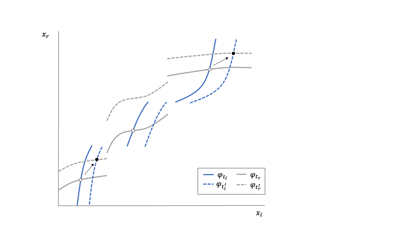
Figure 1: Multiple equilibria comparative statics

Consider now the expected policy function,

$$\pi\left(x_{l},x_{r}\right):=P\left(x_{l},x_{r}\right)x_{l}+\left(1-P\left(x_{l},x_{r}\right)\right)x_{r}.$$

The expected policy function estimates, before the resolution of uncertainty about the electoral outcome, the platform that will ultimately be adopted as policy. The left panel of Figure 2 plots the expected policy as a function of the platform, $x_{i},$ chosen by candidate $i$, given the platform, $x$, chosen by $i$’s opponent. When $x_{i}=0$, $i$’s platform is too extreme to entail a substantial probability of the candidate winning the election, and the expected policy is therefore close to the platform chosen by $i$’s opponent, $x$. As candidate $i$ moderates their platform, starting from zero, $i$’s probability of winning increases, and the expected policy therefore moves away from $x$. Eventually, as $x_{i}$ gets close to $x$, so does the expected policy. Similarly, if $x_{i}=1$ and this platform is too extreme to entail any substantial probability of candidate $i$ winning the election, the expected policy is close to the platform chosen by $i$’s opponent, $x$. As candidate $i$ moderates their platform, starting from one, $i$’s probability of winning grows, and the expected policy then begins to move away from $x$.

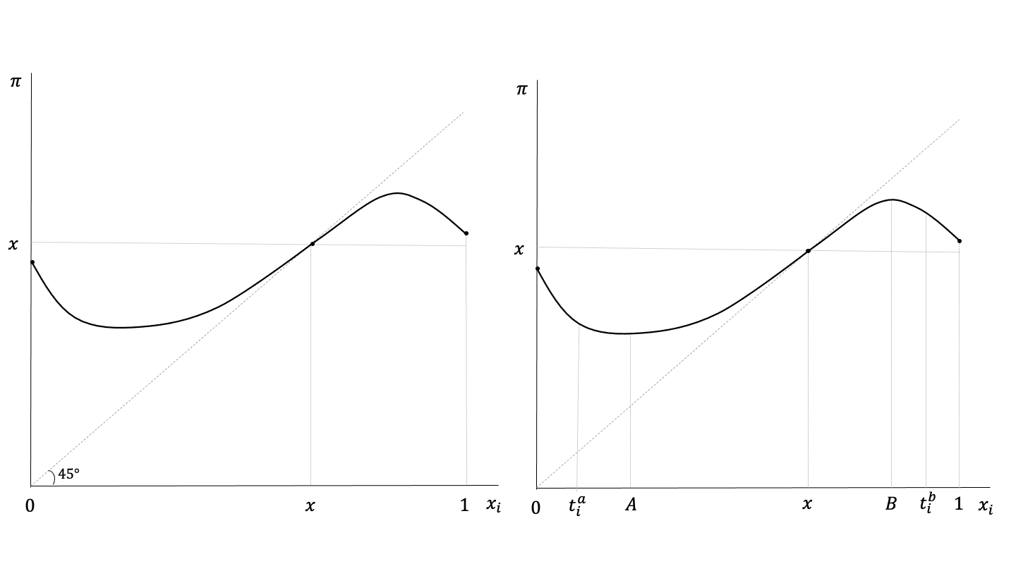
Figure 2: The Expected Policy Function

Theorem 2.

Let $x_{r}>t_{l}$, $x_{l}\in\varphi_{t_{l}}\left(x_{r}\right)$ and $x_{l}^{\prime}>x_{l}$. Then $\pi\left(x_{l}^{\prime},x_{r}\right)>\pi\left(x_{l},x_{r}\right).$ Let $x_{l}<t_{r}$, $x_{r}\in\varphi_{t_{r}}\left(x_{l}\right)$ and $x_{r}^{\prime}<x_{r}$. Then $\pi\left(x_{l},x_{r}^{\prime}\right)<\pi\left(x_{l},x_{r}\right).$

Theorem 2 contains the main insight of the paper: a rational candidate would select a platform that is in the increasing region of the expected policy function. The right panel of Figure 2 illustrates this. If $t_{i}$ is in the increasing region of the expected policy function, the result follows since Lemma 1 shows that $\varphi_{t_{i}}\left(x\right)$is between $t_{i}$ and $x$. Now suppose that candidate $i$’s ideal policy is, say $t_{i}^{a}$ (resp. $t_{i}^{b}$). Then selecting a platform between $t_{i}^{a}$ and $A$ (resp. between $B$ and $t_{i}^{b}$) would leave unexploited the possibility of increasing the expected payoff for the candidate by moderating their platform, as this would drive the expected policy closer to candidate $i$’s ideal point policy while at the same increasing the candidate’s probability of winning the election.

Since the platforms chosen by candidates in equilibrium are endogenous, hypotheses testing that relies on direct estimation of the shape of the expected policy function may be riddled with simultaneity bias. In order to address this issue, we note that the equilibrium indirect expected policy function, which maps candidate preferences into expected policies for a given equilibrium, shares the same comparative statics implications of the expected policy function and can thus be used to investigate whether credibility problems can arise in practice, even in the presence of multiple equilibria.

The equilibrium indirect expected policy function can be computed as follows:

If $\left(x_{l}^{*},x_{r}^{*}\right)\in E$, then

$$\pi^{*}\left(t_{l},t_{r};x_{l}^{*},x_{r}^{*}\right):=\pi\left(x_{l}^{*}\left(t_{l},t_{r}\right),x_{r}^{*}\left(t_{l},t_{r}\right)\right).$$

Let $\overline{\pi}^{*}\left(t_{l},t_{r}\right)$ and $\underline{\pi}^{*}\left(t_{l},t_{r}\right)$ be the equilibrium indirect expected policy corresponding to the largest and smallest equilibrium in $E$, respectively. That is, $\overline{\pi}^{*}\left(t_{l},t_{r}\right)=\pi^{*}\left(t_{l},t_{r};\overline{x}_{l}^{*},\overline{x}_{r}^{*}\right)$ and $\underline{\pi}^{*}\left(t_{l},t_{r}\right)=\pi^{*}\left(t_{l},t_{r};\underline{x}_{l}^{*},\underline{x}_{r}^{*}\right)$

We know from Theorem 2 that in equilibrium the expected policy is increasing in $x_{l}$ and $x_{r}$. From Theorem 1 we know that the largest and smallest Nash equilibria of the game, $\left(\overline{x}_{l},\overline{x}_{r}\right)$ and $\left(\underline{x}_{l},\underline{x}_{r}\right)$, are increasing in $t_{l}$ and $t_{r}.$ It thus follows that the equilibrium indirect expected policy functions associated with the largest and smallest equilibria are also increasing in $t_{l}$ and $t_{r}$. This is the main comparative statics result of the paper, which we summarize below.

Corollary 1.

Assume that SSCP and SLS hold. If $t_{l}^{\prime}>t_{l}$ then $\overline{\pi}^{*}\left(t_{l}^{\prime},t_{r}\right)\geq\overline{\pi}^{*}\left(t_{l},t_{r}\right)$ and $\underline{\pi}^{*}\left(t_{l}^{\prime},t_{r}\right)\geq\underline{\pi}^{*}\left(t_{l},t_{r}\right).$ If $t_{r}^{\prime}<t_{r}$ then $\overline{\pi}^{*}\left(t_{l},t_{r}^{\prime}\right)\leq\overline{\pi}^{*}\left(t_{l},t_{r}\right)$ and $\underline{\pi}^{*}\left(t_{l},t_{r}^{\prime}\right)\leq\underline{\pi}^{*}\left(t_{l},t_{r}\right).$

2.2 A model without commitment

When candidates cannot precommit to adopt a particular platform, voters expect that, if elected, a candidate will implement their most preferred policy once in office. Therefore, the candidates cannot affect the probabilities of being elected and in the unique equilibrium, $x_{l}^{\ast}=t_{l}$ and $x_{r}^{\ast}=t_{r}.$ Because of this, the adopted platforms are trivially increasing in $t_{l}$ and $t_{r}.$

It turns out, however, that in the model without commitment, Theorem 2 fails and hence the indirect expected policy function need not be increasing in the ideal policies of the politicians, as in the model with commitment. We illustrate that this is the case with an example.

Consider a situation where candidates form beliefs about the policy preferred by the median voter, $\mathbf{m},$ as follows: $\mathbf{m}$ is a random variable that is distributed according to a triangular distribution in the [0,1] interval, with mode 0.5. We also let $u\left(x,t\right)=-\left(x-t\right)^{2}$ with $x_{r}>0.5,$ although nothing in the example depends on these choices. We then investigate the behavior of $P\left(x_{l},x_{r}\right)$ as $x_{l}$ varies given a fixed value of $x_{r}$, and of $\pi^{*}\left(t_{l},t_{r}\right)$ as $t_{l}$ varies given a fixed value of $t_{r}$. We obtain that

$$P\left(x_{l},x_{r}\right)=\left\{\begin{array}[]{ccc}2\left(\frac{x_{l}+x_{r}}{2}\right)^{2}&\text{if}&\text{ $x_{l}\leq 1-x_{r}$}\\ 1-2\left(1-\frac{x_{l}+x_{r}}{2}\right)^{2}&\text{if}&\text{}1-x_{r}<x_{l}<x_{r}\\ \frac{1}{2}&\text{if}&x_{l}=x_{r}\\ 2\left(1-\frac{x_{l}+x_{r}}{2}\right)^{2}&\text{if}&x_{l}>x_{r}\end{array}.\right.$$

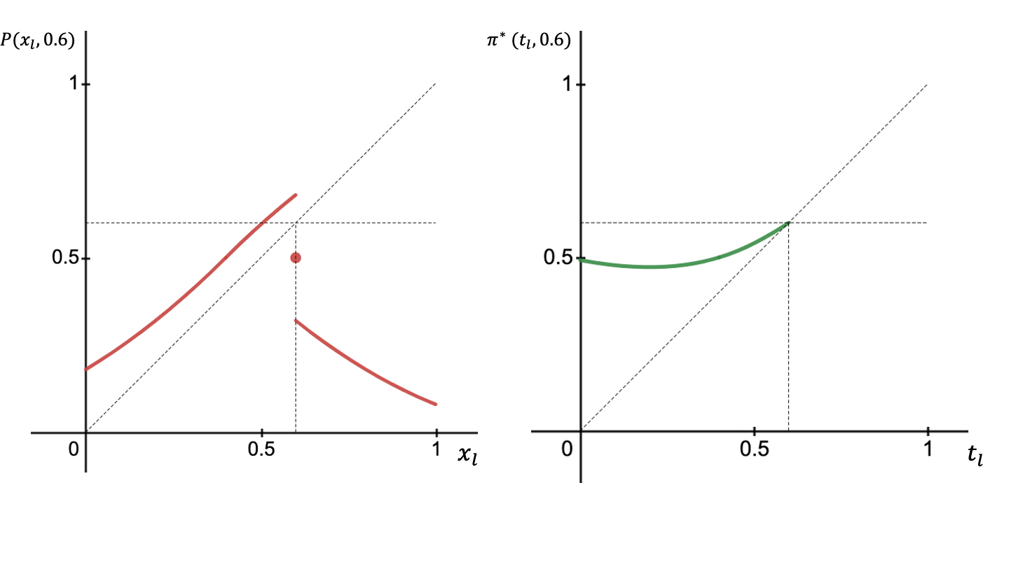
Figure 3: The Model Without Commitment

The left panel of Figure 3 represents the behavior of $P\left(x_{l},x_{r}\right)$ given $x_{r}=0.6,$ and as $x_{l}$ varies from zero to one. As expected, the probability of candidate $l$ winning the election grows as the candidate’s ideal policy approaches $x_{r}=0.6$ from either side, and this probability jumps to $0.5$ when both candidates have the same ideal policies.

The equilibrium indirect expected policy function in this case, when $x_{l}^{\ast}=t_{l}$ and $x_{r}^{\ast}=t_{r},$ can be more simply written as $\pi^{*}\left(t_{l},t_{r};t_{l},t_{r}\right)=\pi^{*}\left(t_{l},t_{r}\right)$, where

$$\pi^{*}\left(t_{l},t_{r}\right)=\left\{\begin{array}[]{ccc}2\left(\frac{t_{l}+t_{r}}{2}\right)^{2}\cdot t_{l}+\left[1-2\left(\frac{t_{l}+t_{r}}{2}\right)^{2}\right]\cdot t_{r}&&\text{if $t_{l}\leq 1-t_{r}$}\\ \left[1-2\left(1-\frac{t_{l}+t_{r}}{2}\right)^{2}\right]\cdot t_{l}+2\left(1-\frac{t_{l}+t_{r}}{2}\right)^{2}\cdot t_{r}&&\text{if }1-t_{r}<t_{l}<t_{r}\\ t_{r}&&\text{if $t_{l}=t_{r}$}\\ 2\left(1-\frac{t_{l}+t_{r}}{2}\right)^{2}\cdot t_{l}+\left[1-2\left(1-\frac{t_{l}+t_{r}}{2}\right)^{2}\right]\cdot t_{r}&&\text{if }t_{l}>t_{r}\end{array},\right.$$

which is a decreasing function of $t_{l}$ when evaluating the function at any $t_{l}<\frac{t_{r}}{3}.$ To see this, notice that, when $t_{l}<1-t_{r},$

$$\frac{d\pi^{*}\left(t_{l},t_{r}\right)}{dt_{l}}=\frac{1}{2}\left(3t_{l}^{2}+2t_{l}t_{r}-t_{r}^{2}\right).$$

We obtain that $\frac{d\pi^{*}\left(0,t_{r}\right)}{dt_{l}}=-t_{r}^{2}<0,$and $\frac{d^{2}\pi^{*}\left(t_{l},t_{r}\right)}{dt_{l}^{2}}=3t_{l}+t_{r}>0$. Therefore, as $t_{l}$ grows from zero, $\frac{d\pi^{*}\left(t_{l},t_{r}\right)}{dt_{l}}$ becomes less negative, until it reaches zero, when $t_{l}=\frac{t_{r}}{3}$, which is the only positive root of $3t_{l}^{2}+2t_{l}t_{r}-t_{r}^{2}$.

Hence, if the ideal point for candidate $l$ happens to be to the left of $\frac{t_{r}}{3},$ the indirect expected policy function will be decreasing in $t_{l}\$ at that point. The right panel of Figure 3 represents the behavior of $\pi^{*}\left(t_{l},t_{r}\right)$ given $t_{r}=0.6,$ and as $t_{l}$ varies from zero to 0.6. The expected policy drops as candidate $l$’s ideal policy approaches 0.2, as explained above, and subsequently rises as candidate l’s ideal policy grows beyond 0.2, and all the way up to 0.6.

As this example shows, it is not hard to find cases in which candidates who cannot make credible commitments will have policy positions that fall on the downward-sloping segment of the indirect expected policy function. This follows from the fact that without a commitment technology, policy platforms will simply reflect candidate preferences. Some candidates have preferences that are so extreme that it would be in their interest to credibly commit to being more moderate if they could do so. That they do not do so is thus good evidence of their inability to credibly make such promises.

This marks an important difference from the commitment case, in which candidates can and do make such promises. In the presence of a commitment technology, extreme candidates will simply decide to moderate their policy platform to the level at which moderation drives the expected policy as close as possible to their ideal point. Therefore, extreme policy positions (in the precise sense of being so extreme that they drive expected policy away from the politician’s ideal point) are inconsistent with rational politicians being able to make credible commitments.

3 Conclusions

We have shown that when candidates can commit to a particular platform during a uni-dimensional electoral contest where valence issues do not arise there must be a positive association between the policies we can expect will be adopted in (the smallest and the largest) equilibrium and the preferred policies held by the candidates. We have also shown that this need not be so if the candidates cannot commit to a particular policy. The implication is that evidence of a negative relationship between enacted and preferred policies in the data is suggestive of candidates that hold positions from which they would like to move from yet are unable to do so. This is the main result of the paper.

This approach can be extended to other models of policy location. For example, Groseclose (2001) proposed a model in which a difference in valence can lead candidates to assume extreme positions. Non-trivial valence differences would violate our symmetry and – under the Groseclose conditions – our monotonicity assumptions, so the approach taken in Section 2 is not directly suitable for testing a valence model. Future research could then focus on (i) allowing for valence and multidimensional issues to play a role, and (ii) understanding what assumptions on the beliefs held by the candidates about the distribution of voter preferences, in lieu of SSCP and SLS, would allow our approach to equilibrium existence and comparative statics to be applicable in these cases.

Our results suggest that empirical work on testing for the existence of credibility problems in politics could advance through direct estimation of the direct and indirect expected policy functions. A regression of enacted policies on policy platforms could shed light on whether the observed correlation between these is positive, as suggested by models of commitment, or negative, as would be the case in citizen-candidate environments. In order to address simultaneity problems in the estimation of the expected policy function, platforms could be instrumented on measures of policymaker or constituent preferences drawn from public opinion surveys, in effect helping us recover the indirect expected policy function.

Anectodally, examples of candidates whose platforms around a single issue were simply too extreme for their own good abound (e.g., George McGovern in 1972 against Richard Nixon and Mario Vargas Llosa in 1990 against Alberto Fujimori). A conventional analysis of the behavior of these politicians would characterize the behavior as relying on gross miscalculations, based on mistaken beliefs about what voters’ actual preferences really were.  Under the alternative interpretation that we espouse, there is nothing irrational about these policy platforms.  It wasn’t the policy platforms of these politicians that cost them the elections: it was their preferences.  Had they proposed more moderate platforms, voters would not have bought it. The presumption that these politicians do not understand the political environment in which they operate is not needed to explain how we see these politicians behaving during election time.

4 References

Alesina, Alberto (1988), “Credibility and Policy Convergence in a Two-candidate System with Rational Voters,” American Economic Review 78, 796-806.

Alesina, Alberto; Nouriel Roubini and Gerald Cohen (1997). Political Cycles and the Macroeconomy. Berkeley: University of California Press.

Enriqueta Aragonès, Andrew Postlewaite, Thomas Palfrey (2007), Political Reputations and Campaign Promises, Journal of the European Economic Association 5(4), 846-884.

Amir, Rabah (2005), “Supermodularity and complementarity in Economics: An Elementary Survey,” Southern Economic Journal 71 (3), 636-660.

Ashworth, Scott and Ethan Bueno de Mesquita (2006), “Monotone Comparative Statics and Models of Politics,” American Journal of Political Science 50, 214-231.

Bagnoli, Mark and Ted Bergstrom (2005), “Log-concave probability and its applications,” Economic Theory 26, 445-469.

Besley, Timothy and Anne Case (1995), “Does Electoral Accountability Affect Economic Policy Choices? Evidence from Gubernatorial Term Limits.” Quarterly Journal of Economics 110 (3), 769-798.

Besley, Timothy and Anne Case (2003), “Political Institutions and Policy Choices: Evidence from the United States.” Journal of Economic Literature 41(1), 7-73.

Besley, Timothy and Stephen Coate (1997), “An Economic Model of Representative Democracy,” Quarterly Journal of Economics 112, 85-114.

Bidwell, Kelly, Katherine Casey and Rachel Glennerster (2020), “Debates: Voting and Expenditure Responses to Political Communication.” Journal of Political Economy 128(8), 2880-2924.

Calvert, Randall (1985), “Robustness of the Multidimensional Voting Model: Candidate Motivations, Uncertainty, and Convergence,” American Journal of Political Science 29, 69-95.

Crain, Mark. (2004), “Dynamic Inconsistency,” in C. Rowley and F. Schneider (eds.), Encyclopaedia of Public Choice, 481-484.

Chattopadhyay, Raghabendra and Esther Duflo (2004), “Women as Policy Makers: Evidence from a Randomized Policy Experiment in India,” Econometrica 72(5), 1409-1443.

Dixit, Avinash, et al. (2000) “The Dynamics of Political Compromise.” Journal of Political Economy 108(3), 531-568.

Duggan, John and César Martinelli (2017), “The Political Economy of Dynamic Elections: Accountability, Commitment and Responsiveness,” Journal of Economic Literature 55, 916-984.

Ferraz, Claudio, and Frederico Finan (2011), “Electoral Accountability and Corruption: Evidence from the Audits of Local Governments,” American Economic Review 101(4), 1274-1311.

Glazer, Amihai (1990), “The Strategy of Candidate Ambiguity,” The American Political Science Review 84(1), 237-241.

Groseclose, Tim (2001), “A Model of Candidate Location When One Candidate Has a Valence Advantage,” American Journal of Political Science 45(4), 862-886.

Hinich, Melvin J. and Michael C. Munger (1997), Analytical Politics. Cambridge: Cambridge University Press.

Kartik, Navin and Preston McAfee, R. P. (2007), “Signaling Character in Electoral Competition”, American Economic Review 97, 852-870.

Navin Kartik and Richard Van Weelden (2018), “Informative Cheap Talk in Elections,” The Review of Economic Studies 86 (2),755-784.

Lee, David. S., Enrico Moretti and Butler, M. J. (2004), “Do Voters Affect or Elect Policies? Evidence from the U.S. House,” Quarterly Journal of Economics 119(3), 807-859.

Mueller, Dennis (2003), Public Choice III. Cambridge: Cambridge University Press.

Osborne, Martin and Al Slivinsky (1996), “A model of Political Competition with Citizen-Candidates,” Quarterly Journal of Economics 111, 64-96.

Panova, Elena (2016), Partially Revealing Campaign Promises. Journal of Public Economic Theory 19(2), 312-330.

Roemer, John (1997), “Political Economic Equilibrium When Parties Represent Constituents: The Unidimensional Case,” Social Choice and Welfare 14, 479-502.

Roemer, John (2001), Political Competition, Cambridge: Harvard University Press.

Shi, Min, and Svensson, Jakob (2006), “Political budget cycles: Do they differ across countries and why?,” Journal of Public Economics 90, 1367-1389.

Sulkin, Tracy (2009), “Campaign Appeals and Legislative Action”, Journal of Politics 71, 1093–1108.

Vives, Xavier (2001), Oligopoly Pricing: Old Ideas and New Tools, MIT Press.

Wittman, Donald (1977), “Candidates with Policy Preferences: A Dynamic Model,” Journal of Economic Theory 14, 180-189.

5 Proofs

Claim 1.

The function $P\left(\pi_{l},\pi_{r}\right)$ satisfies the following properties:

Property $(S)$: For every $x_{l},x_{r}\in T$, $P\left(x_{l},x_{r}\right)=1-P\left(x_{r},x_{l}\right)$.

Property $(M)$: For every $x_{l},x_{l}^{\prime},x_{r}\in T$ with $x_{l}<x_{l}^{\prime}<x_{r}$ , $P\left(x_{l},x_{r}\right)<P\left(x_{l}^{\prime},x_{r}\right)$ and for every $x_{l},x_{l}^{\prime},x_{r}\in T$ with $x_{r}<x_{l}<x_{l}^{\prime}$ , $P\left(x_{l},x_{r}\right)>P\left(x_{l}^{\prime},x_{r}\right).$

Property $(Po)$: For every $x_{l},x_{r}\in T$ , $0<P\left(x_{l},x_{r}\right)<1$.

Proof.

First consider property $(S)$. Let $x_{l},x_{r}\in T$. Then

$$1-P\left(x_{l},x_{r}\right)=\left\{\begin{array}[]{ccc}1-F\left(\frac{x_{l}+x_{r}}{2}\right)&&\text{if }x_{l}<x_{r}\\ \frac{1}{2}&&\text{if $x_{l}=x_{r}$}\\ F\left(\frac{x_{l}+x_{r}}{2}\right)&&\text{if $x_{l}>x_{r}$}\end{array}\right.$$

$$=P\left(x_{r},x_{l}\right),$$

which is what we wanted to show.

Now consider Property $(M)$.

Let $x_{l},x_{l}^{\prime},x_{r}\in T$ with $x_{l}<x_{l}^{\prime}<x_{r}$. Then $P\left(x_{l}^{\prime},x_{r}\right)=F\left(\frac{x_{l}^{\prime}+x_{r}}{2}\right)>F\left(\frac{x_{l}+x_{r}}{2}\right)=P\left(x_{l},x_{r}\right)$, since $F$ is increasing. Now let $x_{l},x_{l}^{\prime},x_{r}\in T$ with $x_{r}<x_{l}<x_{l}^{\prime}$. Again, since $F$ is increasing,

$$P\left(x_{l}^{\prime},x_{r}\right)=1-F\left(\frac{x_{l}^{\prime}+x_{r}}{2}\right)<1-F\left(\frac{x_{l}+x_{r}}{2}\right)=P\left(x_{l},x_{r}\right).$$

Now consider Property $(Po)$. If $x_{l}=x_{r}$, then the result follows, since $P\left(x_{r},x_{l}\right)=1/2$. Now let $x_{l}\neq x_{r}$. Then the result follows since $F$ has full support, which means that, no matter the values of $x_{l}$ and $x_{r}$, there is a positive probability that $\mathbf{m}$ lies in the interval $\left(0,\frac{x_{l}+x_{r}}{2}\right)$ and in the interval $\left(\frac{x_{l}+x_{r}}{2},1\right)$. ∎

Lemma 3.

The best response correspondence $\varphi_{i}$ for candidate i with ideal policy $t_{i}$ and platform, $x$, chosen by i’s opponent has the following properties:

$$\left\{\begin{array}[]{ccc}\varphi_{t_{i}}\left(x\right)\subset(x,t_{i}]&&\text{if $x<t_{i}$}\\ \varphi_{t_{i}}\left(x\right)=\{t_{i}\}&&\text{if $x=t_{i}$}\\ \varphi_{t_{i}}\left(x\right)\subset[t_{i},x)&&\text{if }x>t_{i}\end{array}\right.$$

Proof.

After rearranging terms and eliminating constants that do not depend on candidate $l$’s choice, the candidate’s decision problem simplifies to:

$$\underset{x_{l}}{\max}\hskip 2.84544ptP\left(x_{l},x_{r}\right)\left(u\left(x_{l},t_{l}\right)-u\left(x_{r},t_{l}\right)\right).$$

This function is discontinuous at $x_{l}=x_{r}$, except when $F(x_{r})=0.5$.

Let $x<t_{l}$.

First, notice that, for every $x_{l}\in\left[0,x\right)$, $P\left(x_{l},x\right)\left(u\left(x_{l},t_{l}\right)-u\left(x,t_{l}\right)\right)<0=P\left(x,x\right)\left(u\left(x,t_{l}\right)-u\left(x,t_{l}\right)\right)$. This shows that $\varphi_{t_{l}}\left(x\right)\subset[x,1]$. Next, notice that for any $x_{l}\in\left(x,t_{l}\right]$, we have that

$$P\left(x_{l},x\right)\left(u\left(x_{l},t_{l}\right)-u\left(x,t_{l}\right)\right)>0=P\left(x,x\right)\left(u\left(x,t_{l}\right)-u\left(x,t_{l}\right)\right).$$

This shows that $\varphi_{t_{l}}\left(x\right)\subset(x,1]$. Now notice that, for every $x_{l}\in\left(t_{l},1\right]$,

$$P\left(t_{l},x\right)\left(u\left(t_{l},t_{l}\right)-u\left(x,t_{l}\right)\right)>P\left(x_{l},x\right)\left(u\left(x_{l},t_{l}\right)-u\left(x,t_{l}\right)\right).$$

This is so because, by Property $(M)$, $P\left(t_{l},x\right)>P\left(x_{l},x\right)$ and $u\left(t_{l},t_{l}\right)>u\left(x_{l},t_{l}\right)$. This shows that $\varphi_{t_{l}}\left(x\right)\subset[0,t_{l}]$. We have thus shown that if $x<t_{l}$ then $\varphi_{t_{l}}\left(x\right)\subset(x,t_{l}]$.

Let $x=t_{l}$.

Then clearly $\varphi_{t_{l}}\left(x\right)=\{t_{l}\}$.

Now let $x>t_{l}$.

As before, notice that, for every $x_{l}\in\left(x,1\right]$,

$$P\left(x_{l},x\right)\left(u\left(x_{l},t_{l}\right)-u\left(x,t_{l}\right)\right)<0=P\left(x,x\right)\left(u\left(x,t_{l}\right)-u\left(x,t_{l}\right)\right).$$

This shows that $\varphi_{t_{l}}\left(x\right)\subset[0,x]$. Next, notice that for any $x_{l}\in\left[t_{l},x\right)$ we have that $P\left(x_{l},x\right)\left(u\left(x_{l},t_{l}\right)-u\left(x,t_{l}\right)\right)>0=P\left(x,x\right)\left(u\left(x,t_{l}\right)-u\left(x,t_{l}\right)\right)$. This shows that $\varphi_{t_{l}}\left(x\right)\subset[0,x)$. Now notice that, for every $x_{l}\in\left[0,t_{l}\right)$,

$$P\left(t_{l},x\right)\left(u\left(t_{l},t_{l}\right)-u\left(x,t_{l}\right)\right)>P\left(x_{l},x\right)\left(u\left(x_{l},t_{l}\right)-u\left(x,t_{l}\right)\right).$$

This is so because, by Property $(M)$, $P\left(t_{l},x\right)>P\left(x_{l},x\right)$ and $u\left(t_{l},t_{l}\right)>u\left(x_{l},t_{l}\right)$. This shows that $\varphi_{t_{l}}\left(x\right)\subset[t_{l},1]$. We have thus shown that if $x>t_{l}$ then $\varphi_{t_{l}}\left(x\right)\subset[t_{l},x)$. This completes the proof for $\varphi_{t_{l}}$.

The proof for $\varphi_{t_{r}}$ is similar and we omit it here. ∎

Proposition 3.

Assume that SSCP holds. Then if $t_{l}\leq x_{r}<x_{r}^{\prime}\leq t_{r}$, then we have that $\underline{\varphi}_{t_{l}}\left(x_{r}^{\prime}\right)\geq\overline{\varphi}_{t_{l}}\left(x_{r}\right),$ and if $t_{r}\geq x_{l}^{\prime}>x_{l}\geq t_{l}$, then we have that $\underline{\varphi}_{t_{r}}\left(x_{l}^{\prime}\right)\geq\overline{\varphi}_{t_{r}}\left(x_{l}\right).$

Proof.

Let $t_{l}\leq x_{r}<x_{r}^{\prime}\leq t_{r}$. Let $x_{l}=\overline{\varphi}_{t_{l}}\left(x_{r}\right)\,$ and $x_{l}^{\prime}=\underline{\varphi}_{t_{l}}\left(x_{r}^{\prime}\right).$ By definition of $\overline{\varphi}_{t_{l}}$,

$$U_{t_{l}}\left(x_{l},x_{r}\right)\geq U_{t_{l}}\left(x_{l}^{\prime},x_{r}\right).$$

We want to show that $x_{l}^{\prime}\geq x_{l}.$

If $x_{r}=t_{l}$ then Lemma 1 implies that $x_{l}=t_{l}$ and $x_{l}^{\prime}\in\left[t_{l},x_{r}^{\prime}\right)$, and hence $x_{l}^{\prime}\geq x_{l}.$

If $x_{r}>t_{l},$ then $x_{l}^{\prime}\geq x_{l}$ follows because, if $x_{l}>x_{l}^{\prime}$, Lemma 1 implies that

$$t_{l}\leq x_{l}^{\prime}<x_{l}<x_{r}<x_{r}^{\prime}\leq t_{r}$$

Then, by $SSCP$,

$$U_{t_{l}}\left(x_{l},x_{r}^{\prime}\right)>U_{t_{l}}\left(x_{l}^{\prime},x_{r}^{\prime}\right)$$

which contradicts the fact that $x_{l}^{\prime}\,$ is optimal given $x_{r}^{\prime}$ for a candidate with ideal policy $t_{l}.$ Hence, $x_{l}^{\prime}\geq x_{l}.$

Combining these implications, we obtain that $\underline{\varphi}_{t_{l}}\left(x_{r}^{\prime}\right)\geq\overline{\varphi}_{t_{l}}\left(x_{r}\right)$ when $t_{r}\geq x_{r}^{\prime}>x_{r}\geq t_{l}$.

Now let $t_{l}\leq x_{l}<x_{l}^{\prime}\leq t_{r}$. Let $x_{r}=\overline{\varphi}_{t_{r}}\left(x_{l}\right)\,$ and $x_{r}^{\prime}=\underline{\varphi}_{t_{r}}\left(x_{l}^{\prime}\right).$ By definition of $\overline{\varphi}_{t_{r}}$,

$$U_{t_{r}}\left(x_{l}^{\prime},x_{r}^{\prime}\right)\geq U_{t_{r}}\left(x_{l}^{\prime},x_{r}\right).$$

We want to show that $x_{r}^{\prime}\geq x_{r}.$ If $x_{l}^{\prime}=t_{r}$ then Lemma 1 implies that $x_{r}^{\prime}=t_{r}$ and also that $x_{r}\in\left(x_{l},t_{r}\right]$, and hence $x_{r}\leq x_{r}^{\prime}.$ If $x_{l}^{\prime}<t_{r},$ then $x_{r}^{\prime}\geq x_{r}$ follows because, if $x_{r}>x_{r}^{\prime}$, Lemma 1 implies that

$$t_{l}\leq x_{l}<x_{l}^{\prime}<x_{r}^{\prime}<x_{r}\leq t_{r}$$

Then, by $SSCP$,

$$U_{t_{r}}\left(x_{l},x_{r}^{\prime}\right)>U_{t_{r}}\left(x_{l},x_{r}\right)$$

which contradicts the fact that $x_{r}$ is optimal given $x_{l}$ for a candidate with ideal policy $t_{r}.$ Hence, $x_{r}^{\prime}\geq x_{r}.$

Combining these implications, we obtain that $\underline{\varphi}_{t_{r}}\left(x_{l}^{\prime}\right)\geq\overline{\varphi}_{t_{r}}\left(x_{l}\right)$ when $t_{r}\geq x_{l}^{\prime}>x_{l}\geq t_{l}$. ∎

Proposition 4.

Assume that SSCP holds. Then the set $E$ of Nash equilibria is non-empty and it has (coordinatewise) largest and smallest elements $\left(\overline{x}_{l}^{*},\overline{x}_{r}^{*}\right)$ and $\left(\underline{x}_{l}^{*},\underline{x}_{r}^{*}\right)$.

Proof.

From Lemma 1 we know that that the map $\left(x_{l},x_{r}\right)\mapsto\left[\overline{\varphi}_{t_{l}}\left(x_{r}\right),\overline{\varphi}_{t_{r}}\left(x_{l}\right)\right]$ takes points in $\left[t_{l},t_{r}\right]\times\left[t_{l},t_{r}\right]$ and maps them to $\left[t_{l},t_{r}\right]\times\left[t_{l},t_{r}\right]$, and from Proposition 1 we know the map is non-decreasing in $\left[t_{l},t_{r}\right]\times\left[t_{l},t_{r}\right]$. It follows from Tarski’s fixed point theorem that the set

$$\overline{E}=\left\{\left(x_{l},x_{r}\right):\left(\overline{\varphi}_{t_{l}}\left(x_{r}\right),\overline{\varphi}_{t_{r}}\left(x_{l}\right)\right)\geq\left(x_{l},x_{r}\right)\right\}$$

is non-empty. Since every Nash equilibrium satisfies

$$\left(\overline{\varphi}_{t_{l}}\left(x_{r}\right),\overline{\varphi}_{t_{r}}\left(x_{l}\right)\right)\geq\left(x_{l},x_{r}\right)),$$

then the set of Nash equlibria is non-empty and the greatest element $\left(\overline{x}_{l},\overline{x}_{r}\right)$ of $\overline{E}$ is the greatest Nash equilibrium of the game. The proof for the least element $\left(\underline{x}_{l},\underline{x}_{r}\right)$ is similar and we omit it here. ∎

Lemma 4.

In every equilibrium $(x_{l}^{\ast},x_{r}^{\ast})$, $t_{l}\leq x_{l}^{\ast}<x_{r}^{\ast}\leq t_{r}.$

Proof.

The proof follows from combining the logical implications of the properties of the best responses $\varphi_{t_{l}}$ and $\varphi_{t_{r}}$ as identified in Lemma 1.

First, notice there is no equilibrium $\left(x_{l},x_{r}\right)$ with $x_{r}\leq t_{l}$ or with $x_{l}<t_{l}$. To see this, notice that if $x_{r}\leq t_{l}$ then $x_{r}<x_{l}\leq t_{l}$ since $x_{l}\in\varphi_{t_{l}}\left(x_{r}\right)$ but then $x_{l}<x_{r}\leq t_{r}$ since $x_{r}\in\varphi_{t_{r}}\left(x_{l}\right)$. On the other hand, $x_{l}<t_{l}$ is only a best response for $l$ if $x_{r}<t_{l}$, which we just showed cannot arise in equilibrium. Therefore, $x_{l}<t_{l}$ also cannot arise in equilibrium.

Similarly, notice there is no equilibrium $\left(x_{l},x_{r}\right)$ with $x_{l}\geq t_{l}$ or with $x_{r}>t_{r}$. To see this, notice that if $x_{l}\geq t_{r}$ then $t_{r}\leq x_{r}<x_{l}$ since $x_{r}\in\varphi_{t_{r}}\left(x_{l}\right)$ but then $t_{l}\leq x_{l}<x_{r}$ since $x_{l}\in\varphi_{t_{l}}\left(x_{r}\right)$. On the other hand, $x_{r}>t_{r}$ is only a best response for $r$ if $x_{l}>t_{r}$, which we just showed cannot arise in equilibrium. Therefore, $x_{r}>t_{r}$ also cannot arise in equilibrium.

Then, in equilibrium, $t_{l}\leq x_{l}<t_{r}$ and $t_{l}<x_{r}\leq t_{r}$. It then follows that $t_{l}\leq x_{l}<x_{r}$ since $x_{l}\in\varphi_{t_{l}}\left(x_{r}\right)$.

We have thus established that, in equilibrium, $t_{l}\leq x_{l}^{\ast}<x_{r}^{\ast}\leq t_{r}$. ∎

Claim 2.

Assume that $SLS$ holds. If $t_{l}<t_{l}^{\prime}\leq x_{l}<x_{l}^{\prime}<x_{r}$ then

$$U_{t_{l}}\left(x_{l}^{\prime},x_{r}\right)\geq U_{t_{l}}\left(x_{l},x_{r}\right)\Rightarrow U_{t_{l}^{\prime}}\left(x_{l}^{\prime},x_{r}\right)>U_{t_{l}^{\prime}}\left(x_{l},x_{r}\right),$$

and if $x_{l}<x_{r}<x_{r}^{\prime}\leq t_{r}<t_{r}^{\prime}$ then

$$U_{t_{r}}\left(x_{l},x_{r}^{\prime}\right)\geq U_{t_{r}}\left(x_{l},x_{r}\right)\Rightarrow U_{t_{r}^{\prime}}\left(x_{l},x_{r}^{\prime}\right)>U_{t_{r}^{\prime}}\left(x_{l},x_{r}\right).$$

Proof.

Let $t_{l}<t_{l}^{\prime}\leq x_{l}<x_{l}^{\prime}<x_{r}$.

Assume that $U_{t_{l}}\left(x_{l}^{\prime},x_{r}\right)\geq U_{t_{l}}\left(x_{l},x_{r}\right)$. By the definition of $U$,

$$P\left(x_{l}^{\prime},x_{r}\right)u\left(x_{l}^{\prime},t_{l}\right)+\left(1-P\left(x_{l}^{\prime},x_{r}\right)\right)u\left(x_{r},t_{l}\right)\geq$$

$$P\left(x_{l},x_{r}\right)u\left(x_{l},t_{l}\right)+\left(1-P_{l}\left(x_{l},x_{r}\right)\right)u\left(x_{r},t_{l}\right),$$

which boils down to

$$\frac{P\left(x_{l}^{\prime},x_{r}\right)}{P\left(x_{l},x_{r}\right)}\frac{\left[u\left(x_{l}^{\prime},t_{l}\right)-u\left(x_{r},t_{l}\right)\right]}{\left[u\left(x_{l},t_{l}\right)-u\left(x_{r},t_{l}\right)\right]}\geq 1.$$

By $SLS$, we have that

$$\frac{u\left(x_{l}^{\prime},t_{l}^{\prime}\right)-u\left(x_{r},t_{l}^{\prime}\right)}{u\left(x_{l},t_{l}^{\prime}\right)-u\left(x_{r},t_{l}^{\prime}\right)}>\frac{u\left(x_{l}^{\prime},t_{l}\right)-u\left(x_{r},t_{l}\right)}{u\left(x_{l},t_{l}\right)-u\left(x_{r},t_{l}\right)},$$

therefore

$$\frac{P\left(x_{l}^{\prime},x_{r}\right)}{P\left(x_{l},x_{r}\right)}\frac{\left[u\left(x_{l}^{\prime},t_{l}^{\prime}\right)-u\left(x_{r},t_{l}^{\prime}\right)\right]}{\left[u\left(x_{l},t_{l}^{\prime}\right)-u\left(x_{r},t_{l}^{\prime}\right)\right]}>\frac{P\left(x_{l}^{\prime},x_{r}\right)}{P\left(x_{l},x_{r}\right)}\frac{\left[u\left(x_{l}^{\prime},t_{l}\right)-u\left(x_{r},t_{l}\right)\right]}{\left[u\left(x_{l},t_{l}\right)-u\left(x_{r},t_{l}\right)\right]},$$

which means that

$$\frac{P\left(x_{l}^{\prime},x_{r}\right)}{P\left(x_{l},x_{r}\right)}\frac{\left[u\left(x_{l}^{\prime},t_{l}^{\prime}\right)-u\left(x_{r},t_{l}^{\prime}\right)\right]}{\left[u\left(x_{l},t_{l}^{\prime}\right)-u\left(x_{r},t_{l}^{\prime}\right)\right]}>1,$$

from where it follows that

$$U_{t_{l}^{\prime}}\left(x_{l}^{\prime},x_{r}\right)>U_{t_{l}^{\prime}}\left(x_{l},x_{r}\right).$$

Now let $x_{l}<x_{r}<x_{r}^{\prime}\leq t_{r}<t_{r}^{\prime}$.

Assume that $U_{t_{r}}\left(x_{l},x_{r}^{\prime}\right)\geq U_{t_{r}}\left(x_{l},x_{r}\right)$. By the definition of $U$,

$$P\left(x_{l},x_{r}^{\prime}\right)u\left(x_{l},t_{r}\right)+\left(1-P\left(x_{l},x_{r}^{\prime}\right)\right)u\left(x_{r}^{\prime},t_{r}\right)\geq$$

$$P\left(x_{l},x_{r}\right)u\left(x_{l},t_{r}\right)+\left(1-P_{l}\left(x_{l},x_{r}\right)\right)u\left(x_{r},t_{r}\right),$$

which boils down to

$$\frac{\left[1-P\left(x_{l},x_{r}^{\prime}\right)\right]}{\left[1-P\left(x_{l},x_{r}\right)\right]}\frac{u\left(x_{r}^{\prime},t_{r}\right)-u\left(x_{l},t_{r}\right)}{u\left(x_{r},t_{r}\right)-u\left(x_{l},t_{r}\right)}\geq 1.$$

By $SLS$, we have that

$$\frac{u\left(x_{r}^{\prime},t_{r}^{\prime}\right)-u\left(x_{l},t_{r}^{\prime}\right)}{u\left(x_{r},t_{r}^{\prime}\right)-u\left(x_{l},t_{r}^{\prime}\right)}>\frac{u\left(x_{r}^{\prime},t_{r}\right)-u\left(x_{l},t_{r}\right)}{u\left(x_{r},t_{r}\right)-u\left(x_{l},t_{r}\right)},$$

therefore

$$\frac{\left[1-P\left(x_{l},x_{r}^{\prime}\right)\right]}{\left[1-P\left(x_{l},x_{r}\right)\right]}\frac{u\left(x_{r}^{\prime},t_{r}^{\prime}\right)-u\left(x_{l},t_{r}^{\prime}\right)}{u\left(x_{r},t_{r}^{\prime}\right)-u\left(x_{l},t_{r}^{\prime}\right)}>\frac{\left[1-P\left(x_{l},x_{r}^{\prime}\right)\right]}{\left[1-P\left(x_{l},x_{r}\right)\right]}\frac{u\left(x_{r}^{\prime},t_{r}\right)-u\left(x_{l},t_{r}\right)}{u\left(x_{r},t_{r}\right)-u\left(x_{l},t_{r}\right)},$$

which means that

$$\frac{\left[1-P\left(x_{l},x_{r}^{\prime}\right)\right]}{\left[1-P\left(x_{l},x_{r}\right)\right]}\frac{u\left(x_{r}^{\prime},t_{r}^{\prime}\right)-u\left(x_{l},t_{r}^{\prime}\right)}{u\left(x_{r},t_{r}^{\prime}\right)-u\left(x_{l},t_{r}^{\prime}\right)}>1,$$

from where it follows that

$$U_{t_{r}^{\prime}}\left(x_{l},x_{r}^{\prime}\right)>U_{t_{r}^{\prime}}\left(x_{l},x_{r}\right).$$

∎

Theorem 3.

Assume that SSCP and SLS hold. Let $t_{l}<t_{l}^{\prime}<t_{r}<t_{r}^{\prime}$. Then

• $\overline{x}_{l}^{*}\left(t_{l}^{\prime},t_{r}\right)\geq\overline{x}_{l}^{*}\left(t_{l},t_{r}\right)$ and $\overline{x}_{r}^{*}\left(t_{l},t_{r}^{\prime}\right)\geq\overline{x}_{r}^{*}\left(t_{l},t_{r}\right)$

• $\underline{x}_{l}^{*}\left(t_{l}^{\prime},t_{r}\right)\geq\underline{x}_{l}^{*}\left(t_{l},t_{r}\right)$ and $\underline{x}_{r}^{*}\left(t_{l},t_{r}^{\prime}\right)\geq\underline{x}_{r}^{*}\left(t_{l},t_{r}\right)$

Proof.

Let $t_{l}<t_{l}^{\prime}.$ Fix $x_{r}>t_{l}$, and let $x_{l}\in\varphi_{t_{l}}\left(x_{r}\right)$. Notice that, by Lemma 1, $x_{l}\in\left[t_{l},x_{r}\right)$. Let $x_{l}^{\prime}\in\varphi_{t_{l}^{\prime}}\left(x_{r}\right).$ We want to show that $x_{l}^{\prime}\geq x_{l}$.

If $t_{l}^{\prime}\geq x_{l}$, then Lemma 1 implies that either $x_{l}^{\prime}\in\left[t_{l}^{\prime},x_{r}\right)$ or $x_{l}^{\prime}\in\left(x_{r},t_{l}^{\prime}\right]$, and either way $x_{l}^{\prime}\geq x_{l}$.

Now assume that $t_{l}^{\prime}\in\left(t_{l},x_{l}\right)$. By definition of $\varphi_{t_{l}}$,

$$U_{t_{l}}\left(x_{l},x_{r}\right)\geq U_{t_{l}}\left(x_{l}^{\prime},x_{r}\right).$$

We argue that $x_{l}^{\prime}\geq x_{l}.$ Assume not, that is, assume that $x_{l}^{\prime}<x_{l}$. Then we obtain that $t_{l}<t_{l}^{\prime}\leq x_{l}^{\prime}<x_{l}<x_{r}$ and, by Claim 2,

$$U_{t_{l}^{\prime}}\left(x_{l},x_{r}\right)>U_{t_{l}^{\prime}}\left(x_{l}^{\prime},x_{r}\right)$$

which contradicts the fact that $x_{l}^{\prime}\,$ is optimal given $x_{r}\$ for a candidate with ideal policy $t_{l}^{\prime}.$ Hence, $x_{l}^{\prime}\geq x_{l}$ (and, in particular, $\overline{\varphi}_{t_{l}^{\prime}}\left(x_{r}\right)\geq\overline{\varphi}_{t_{l}}\left(x_{r}\right)$ and $\underline{\varphi}_{t_{l}^{\prime}}\left(x_{r}\right)\geq\underline{\varphi}_{t_{l}}\left(x_{r}\right)$) when $x_{r}>t_{l}$.

Let $t_{r}<t_{r}^{\prime}$. Fix $x_{l}<t_{r}^{\prime}$ and let $x_{r}^{\prime}\in\varphi_{t_{r}^{\prime}}\left(x_{l}\right)$. By Lemma 1, $x_{r}^{\prime}\in\left(x_{l},t_{r}^{\prime}\right]$. Let $x_{r}\in\varphi_{t_{r}}\left(x_{l}\right).$ We now want to show that $x_{r}^{\prime}\geq x_{r}.$

If $t_{r}\leq x_{r}^{\prime}$, then Lemma 1 implies that either $x_{r}\in\left[t_{r},x_{l}\right)$ or $x_{r}\in\left(x_{l},t_{r}\right]$, and either way $x_{r}^{\prime}\geq x_{r}$.

Now assume that $t_{r}\in\left(x_{r}^{\prime},t_{r}^{\prime}\right)$. By definition of $\varphi_{t_{r}^{\prime}}$,

$$U_{t_{r}^{\prime}}\left(x_{l},x_{r}^{\prime}\right)\geq U_{t_{r}^{\prime}}\left(x_{l},x_{r}\right)$$

We argue that $x_{r}^{\prime}\geq x_{r}.$ Assume not, that is, assume that $x_{r}^{\prime}<x_{r}$. We then obtain that $x_{l}<x_{r}^{\prime}<x_{r}\leq t_{r}<t_{r}^{\prime}$ and, by Claim 2,

$$U_{t_{r}}\left(x_{l},x_{r}^{\prime}\right)>U_{t_{r}}\left(x_{l},x_{r}\right)$$

which contradicts the fact that $x_{r}$ is optimal given $x_{l}\$ for a candidate with ideal policy $t_{r}.$ Hence, $x_{r}^{\prime}\geq x_{r}$ (and, in particular, $\overline{\varphi}_{t_{r}^{\prime}}\left(x_{l}\right)\geq\overline{\varphi}_{t_{r}}\left(x_{l}\right)$ and $\underline{\varphi}_{t_{r}^{\prime}}\left(x_{l}\right)\geq\underline{\varphi}_{t_{r}}\left(x_{l}\right)$) for $t_{r}^{\prime}>x_{l}$.

Let $\overline{x}^{*}\left(t_{l},t_{r}\right)=\sup\left\{\left(x_{l},x_{r}\right):\left(\overline{\varphi}_{t_{l}}\left(x_{r}\right),\overline{\varphi}_{t_{r}}\left(x_{l}\right)\right)\geq\left(x_{l},x_{r}\right)\right\}$ be the largest fixed point of $\left(x_{l},x_{r}\right)\mapsto\left[\overline{\varphi}_{t_{l}}\left(x_{r}\right),\overline{\varphi}_{t_{r}}\left(x_{l}\right)\right]$, and therefore the largest Nash equilibrium of the game. This equilibrium exists, by Proposition 2.

By Lemma 2, $t_{l}\leq\overline{x}_{l}^{*}\left(t_{l},t_{r}\right)<\overline{x}_{r}^{*}\left(t_{l},t_{r}\right)\leq t_{r}.$

We obtain that $\overline{x}_{r}^{*}\left(t_{l},t_{r}\right)>t_{l}$ and therefore $\overline{x}_{l}^{*}\left(t_{l}^{\prime},t_{r}\right)\geq\overline{x}_{l}^{*}\left(t_{l},t_{r}\right)$. Similarly, we obtain that $t_{r}^{\prime}>\overline{x}_{l}^{*}\left(t_{l},t_{r}\right)$ and therefore $\overline{x}_{r}^{*}\left(t_{l},t_{r}^{\prime}\right)\geq\overline{x}_{r}^{*}\left(t_{l},t_{r}\right)$ since we just showed that $\overline{\varphi}_{t_{l}^{\prime}}\left(x_{r}\right)\geq\overline{\varphi}_{t_{l}}\left(x_{r}\right)$ when $x_{r}>t_{l}$, and $\overline{\varphi}_{t_{r}^{\prime}}\left(x_{l}\right)\geq\overline{\varphi}_{t_{r}}\left(x_{l}\right)$ when $t_{r}^{\prime}>x_{l}.$ The case of the smallest equilibrium is analogous. ∎

Theorem 4.

Let $x_{r}>t_{l}$, $x_{l}\in\varphi_{t_{l}}\left(x_{r}\right)$ and $x_{l}^{\prime}>x_{l}$. Then $\pi\left(x_{l}^{\prime},x_{r}\right)>\pi\left(x_{l},x_{r}\right).$ Let $x_{l}<t_{r}$, $x_{r}\in\varphi_{t_{r}}\left(x_{l}\right)$ and $x_{r}^{\prime}<x_{r}$. Then $\pi\left(x_{l},x_{r}^{\prime}\right)<\pi\left(x_{l},x_{r}\right).$

Proof.

We first establish the result for changes in $x_{l}$ while keeping $x_{r}$ fixed. Let $x_{r}>t_{l}$ and $x_{l}\in\varphi_{t_{l}}\left(x_{r}\right).$ From Lemma 1 we know that $t_{l}\leq x_{l}<x_{r}$. If $x_{l}^{\prime}\geq x_{r}$ the result follows immediately since

$$P\left(x_{l}^{\prime},x_{r}\right)x_{l}^{\prime}+\left(1-P\left(x_{l}^{\prime},x_{r}\right)\right)x_{r}>P\left(x_{l},x_{r}\right)x_{l}+\left(1-P\left(x_{l},x_{r}\right)\right)x_{r}$$

regardless of the value of $P\left(x_{l}^{\prime},x_{r}\right)$ and $P\left(x_{l},x_{r}\right)$, which are always positive.

Now let $x_{l}^{\prime}\in\left(x_{l},x_{r}\right).$ We want to show that $\pi\left(x_{l}^{\prime},x_{r}\right)>\pi\left(x_{l},x_{r}\right).$

Assume not, that is, assume that

$$P\left(x_{l}^{\prime},x_{r}\right)x_{l}^{\prime}+\left(1-P\left(x_{l}^{\prime},x_{r}\right)\right)x_{r}\leq P\left(x_{l},x_{r}\right)x_{l}+\left(1-P\left(x_{l},x_{r}\right)\right)x_{r}.$$

Cancelling and rearranging terms yields

$$\frac{P\left(x_{l}^{\prime},x_{r}\right)}{P\left(x_{l},x_{r}\right)}\geq\frac{x_{r}-x_{l}}{x_{r}-x_{l}^{\prime}}.$$

Since $x_{l}\in\varphi_{t_{l}}\left(x_{r}\right)$, it follows that

$$P\left(x_{l},x_{r}\right)u\left(x_{l},t_{l}\right)+\left(1-P\left(x_{l},x_{r}\right)\right)u\left(x_{r},t_{l}\right)\geq$$

$$P\left(x_{l}^{\prime},x_{r}\right)u\left(x_{l}^{\prime},t_{l}\right)+\left(1-P\left(x_{l}^{\prime},x_{r}\right)\right)u\left(x_{r},t_{l}\right).$$

We obtain that

$$\frac{P\left(x_{l}^{\prime},x_{r}\right)}{P\left(x_{l},x_{r}\right)}\leq\frac{u\left(x_{r},t_{l}\right)-u\left(x_{l},t_{l}\right)}{u\left(x_{r},t_{l}\right)-u\left(x_{l}^{\prime},t_{l}\right)}.$$

Putting these expressions together yields

$$\frac{u\left(x_{r},t_{l}\right)-u\left(x_{l},t_{l}\right)}{u\left(x_{r},t_{l}\right)-u\left(x_{l}^{\prime},t_{l}\right)}\geq\frac{x_{r}-x_{l}}{x_{r}-x_{l}^{\prime}},$$

which is equivalent to

$$u\left(x_{l}^{\prime},t_{l}\right)\leq\frac{x_{r}-x_{l}^{\prime}}{x_{r}-x_{l}}u\left(x_{l},t_{l}\right)+\left(1-\frac{x_{r}-x_{l}^{\prime}}{x_{r}-x_{l}}\right)u\left(x_{r},t_{l}\right).$$ (1)

But $\frac{x_{r}-x_{l}^{\prime}}{x_{r}-x_{l}}x_{l}+\left(1-\frac{x_{r}-x_{l}^{\prime}}{x_{r}-x_{l}}\right)x_{r}=x_{l}^{\prime}$ and $\frac{x_{r}-x_{l}^{\prime}}{x_{r}-x_{l}}\in\left(0,1\right)$. Therefore, strict concavity requires that

$$u\left(x_{l}^{\prime},t_{l}\right)>\frac{x_{r}-x_{l}^{\prime}}{x_{r}-x_{l}}u\left(x_{l},t_{l}\right)+\left(1-\frac{x_{r}-x_{l}^{\prime}}{x_{r}-x_{l}}\right)u\left(x_{r},t_{l}\right).$$ (2)

The contradiction between equations (1) and (2) establishes the first result.

Now we establish the result for changes in $x_{r}$ while keeping $x_{l}$ fixed.

Let $x_{l}<t_{r}$, $x_{r}\in\varphi_{t_{r}}\left(x_{l}\right)$ and $x_{r}^{\prime}<x_{r}$. From Lemma 1 we know that $x_{l}<x_{r}\leq t_{r}$. If $x_{r}^{\prime}\leq x_{l}$ the result follows immediately since

$$P\left(x_{l},x_{r}^{\prime}\right)x_{l}+\left(1-P\left(x_{l},x_{r}^{\prime}\right)\right)x_{r}^{\prime}<P\left(x_{l},x_{r}\right)x_{l}+\left(1-P\left(x_{l},x_{r}\right)\right)x_{r}$$

regardless of the value of the probabilities $P\left(x_{l},x_{r}^{\prime}\right)$ and $P\left(x_{l},x_{r}\right)$, which are always positive.

Now let $x_{r}^{\prime}\in\left(x_{l},x_{r}\right).$ We want to show that $\pi\left(x_{l},x_{r}^{\prime}\right)<\pi\left(x_{l},x_{r}\right).$

Assume not, that is, assume that

$$P\left(x_{l},x_{r}^{\prime}\right)x_{l}+\left(1-P\left(x_{l},x_{r}^{\prime}\right)\right)x_{r}^{\prime}\geq P\left(x_{l},x_{r}\right)x_{l}+\left(1-P\left(x_{l},x_{r}\right)\right)x_{r}.$$

Cancelling and rearranging terms yields

$$\frac{1-P\left(x_{l},x_{r}^{\prime}\right)}{1-P\left(x_{l},x_{r}\right)}\geq\frac{x_{r}-x_{l}}{x_{r}^{\prime}-x_{l}}.$$

Since $x_{r}\in\varphi_{t_{r}}\left(x_{l}\right)$, it follows that

$$P\left(x_{l},x_{r}\right)u\left(x_{l},t_{r}\right)+\left(1-P\left(x_{l},x_{r}\right)\right)u\left(x_{r},t_{r}\right)\geq$$

$$P\left(x_{l},x_{r}^{\prime}\right)u\left(x_{l},t_{l}\right)+\left(1-P\left(x_{l},x_{r}^{\prime}\right)\right)u\left(x_{r}^{\prime},t_{l}\right).$$

We obtain that

$$\frac{1-P\left(x_{l},x_{r}^{\prime}\right)}{1-P\left(x_{l},x_{r}\right)}\leq\frac{u\left(x_{r},t_{r}\right)-u\left(x_{l},t_{r}\right)}{u\left(x_{r}^{\prime},t_{r}\right)-u\left(x_{l},t_{r}\right)}.$$

Putting these expressions together yields

$$\frac{u\left(x_{r},t_{r}\right)-u\left(x_{l},t_{r}\right)}{u\left(x_{r}^{\prime},t_{r}\right)-u\left(x_{l},t_{r}\right)}\geq\frac{x_{r}-x_{l}}{x_{r}^{\prime}-x_{l}},$$

which is equivalent to

$$u\left(x_{r}^{\prime},t_{r}\right)\leq\frac{x_{r}^{\prime}-x_{l}}{x_{r}-x_{l}}u\left(x_{r},t_{r}\right)+\left(1-\frac{x_{r}^{\prime}-x_{l}}{x_{r}-x_{l}}\right)u\left(x_{l},t_{r}\right).$$ (3)

But $\frac{x_{r}^{\prime}-x_{l}}{x_{r}-x_{l}}x_{r}^{\prime}+\left(1-\frac{x_{r}^{\prime}-x_{l}}{x_{r}-x_{l}}\right)x_{l}=x_{r}^{\prime}$ and $\frac{x_{r}^{\prime}-x_{l}}{x_{r}-x_{l}}\in\left(0,1\right)$. Therefore, strict concavity requires that

$$u\left(x_{r}^{\prime},t_{r}\right)>\frac{x_{r}^{\prime}-x_{l}}{x_{r}-x_{l}}u\left(x_{r},t_{r}\right)+\left(1-\frac{x_{r}^{\prime}-x_{l}}{x_{r}-x_{l}}\right)u\left(x_{l},t_{r}\right).$$ (4)

The contradiction between equations (3) and (4) establishes the second result. ∎