Relaxation-speed crossover in anharmonic potentials

Abstract

In a recent Letter [A. Lapolla and A. Godec, Phys. Rev. Lett. 125, 110602 (2020)], thermal relaxation was observed to occur faster from cold to hot (heating) than from hot to cold (cooling). Here we show that overdamped diffusion in anharmonic potentials generically exhibits both faster heating and faster cooling, depending on the initial temperatures and on the potential’s degree of anharmonicity. We draw a relaxation-speed phase diagram that localises the different behaviours in parameter space. In addition to faster-heating and faster-cooling regions, we identify a crossover region in the phase diagram, where heating is initially slower but asymptotically faster than cooling. The structure of the phase diagram is robust against the inclusion of a confining, harmonic term in the potential as well as moderate changes of the measure used to define initially equidistant temperatures.

Many thermal relaxation processes in nature and industry occur out of equilibrium, and thus outside of the realm of the quasistatic approximation. As a consequence, nonequilibrium thermal relaxation gives rise to anomalous effects, such as ergodicity breaking Bray (2002) or the Mpemba effect Mpemba and Osborne (1969). The latter describes the surprising observation that some systems cool down faster, when relaxing from a higher initial temperature. A better understanding of such anomalous relaxation effects in out-of-equilibrium systems is important, because it may allow us to use these phenomena to our advantage, for instance, for increasing the rate of heating and cooling.

Although a complete understanding of anomalous relaxation in macroscopic systems appears elusive at present, much progress has been made recently in reproducing anomalous relaxation phenomena on mesoscopic scales. This has led to several important results such as new theoretical Lu and Raz (2017); Klich et al. (2019); Walker and Vucelja (2021); Chétrite et al. (2021) and experimental Kumar and Bechhoefer (2020); Kumar et al. (2021) insights into the Mpemba effect, strategies to increase the rate at which systems can be cooled Gal and Raz (2020); Prados (2021); Carollo et al. (2021), and an information-theoretic bound on the speed of relaxation to equilibrium Shiraishi and Saito (2019).

Within a setup closely related to, yet slightly different from, the Mpemba effect, a recent study Lapolla and Godec (2020) reported an asymmetry in the rate at which systems heat up and cool down. According to this study, and subsequent works by other authors, heating occurs faster than cooling for diffusive systems with harmonic potentials Lapolla and Godec (2020) and for discrete-state two-level systems Manikandan (2021); Van Vu and Hasegawa (2021). On the other hand, it was shown that this relaxation asymmetry is non-generic for diffusion in potentials with multiple minima Lapolla and Godec (2020) or in discrete-state systems with more than two states Manikandan (2021); Van Vu and Hasegawa (2021). However, it appears to be widely believed that the described effect is a general property of overdamped, diffusive systems with stable single-well potentials Lapolla and Godec (2020); Manikandan (2021); Van Vu and Hasegawa (2021).

In this Letter, we study the relaxation asymmetry for overdamped diffusion in anharmonic potentials. Opposing common belief, we show that these systems exhibit both behaviours, faster heating and faster cooling, even for stable single-well potentials. Based on these results, we draw a phase diagram locating the different regions of “faster heating” and “faster cooling” in parameter space. These two regions are separated by a crossover region where cooling occurs faster at first, but heating overtakes at a finite time. Our results suggest that the relative speed of thermal relaxation to equilibrium can be substantially increased by varying the anharmonicity of the potential. This should be testable in experiments and has potential applications in the optimisation of cooling strategies for small-scale systems Gal and Raz (2020).

To specify the problem, consider two equilibrium systems, otherwise identical, but at different temperatures $T_{c}<T_{h}$. We call the system at temperature $T_{c}$ cold and that at temperature $T_{h}$ hot. At time $t=0$, both systems experience an instantaneous temperature quench to the same final temperature $T_{f}$, where $T_{c}<T_{f}<T_{h}$. The relaxation of the two systems toward equilibrium is monitored by their nonequilibrium free-energy difference Lapolla and Godec (2020),

$$\mathcal{F}_{i}(t)= \left\langle\Delta E_{i}(t)\right\rangle-T_{f}\left\langle\Delta S_{i}(t)\right\rangle\,,$$

$$= k_{\text{B}}T_{f}\int_{-\infty}^{\infty}\!\!\text{d}x\,p_{i}(x,t)\ln\left[\frac{p_{i}(x,t)}{p_{f}(x)}\right]\,,$$ (1)

with respect to the equilibrium distribution $p_{f}$ at final temperature $T_{f}$. Here, $\left\langle\Delta E_{i}(t)\right\rangle$ and $\left\langle\Delta S_{i}(t)\right\rangle$ are the average differences in the energy and entropy of the (cold or hot) system at time $t$ and its equilibrium state at temperature $T_{f}$; $k_{\text{B}}$ denotes the Boltzmann constant. The index $i$ in Eq. (Relaxation-speed crossover in anharmonic potentials) takes the values $c$ and $h$, and $p_{c}$ and $p_{h}$ denote the probability densities of the initially cold and hot system, respectively.

In order to quantitatively compare the distances $\mathcal{F}_{i}(t)$ from equilibrium, the temperatures $T_{c}$ and $T_{h}$ at $t=0$ are chosen so that $\mathcal{F}_{c}(0)=\mathcal{F}_{h}(0)$ Lapolla and Godec (2020). We call such a temperature quench “$\mathcal{F}$-equidistant,” i.e., at equal distance with respect to the temperature measure (Relaxation-speed crossover in anharmonic potentials). A comparison between this setup and the Markovian Mpemba effect Lu and Raz (2017); Klich et al. (2019) is made in Sec. I of the Supplemental Material (SM) SM .

The specific measure (Relaxation-speed crossover in anharmonic potentials) is used for two reasons. First, $\mathcal{F}_{i}$ is a thermodynamic quantity for systems at equilibrium and hence for $t<0$ and in the limit $t\to\infty$. Second, it remains well defined out of equilibrium and thus for all finite times $t$.

In the long-time limit, both the cold and the hot system relax to equilibrium so that $\mathcal{F}_{c}(t)$ and $\mathcal{F}_{h}(t)$ tend to zero asymptotically. The relative distance from equilibrium of the two systems is conveniently measured by the logarithmic ratio

$$\mathcal{R}(t)\equiv\ln\left[\frac{\mathcal{F}_{h}(t)}{\mathcal{F}_{c}(t)}\right]\,.$$ (2)

For overdamped diffusion in a harmonic potential, one can prove that $\mathcal{R}(t)>0$, i.e., $\mathcal{F}_{h}(t)>\mathcal{F}_{c}(t)$ during the relaxation Lapolla and Godec (2020), i.e., heating occurs faster than cooling; $\mathcal{R}(t)<0$ corresponds to the opposite case, that of faster cooling. Note also that $\mathcal{R}(0)=0$ by definition of $\mathcal{F}$ equidistance, $\mathcal{F}_{c}(0)=\mathcal{F}_{h}(0)$. Hence, the momentary, relative distance from equilibrium is determined by the sign of $\mathcal{R}(t)$.

We study the evolution of $\mathcal{R}(t)$ for overdamped diffusion in an anharmonic potential $V(x)$. For simplicity, we analyse the case of one spatial dimension and assume $V(x)$ to be of the form $V(x)=\lambda x^{2}+k|x|^{\alpha}$, where we consider parameter values $\lambda$, $k$ and $\alpha$ for which $V$ is confining, $V(x)\to\infty$ as $x\to\pm\infty$. We move to a dimensionless formulation by defining a timescale $\tau$ and a length scale $\ell$ as

$$\tau=\frac{1}{\mu k_{\text{B}}T_{f}}\left(\frac{k}{k_{\text{B}}T_{f}}\right)^{-2/\alpha}\,,\quad\ell=\left(\frac{k}{k_{\text{B}}T_{f}}\right)^{-1/\alpha}\,.$$ (3)

Here, $\mu$ is the mobility. In the dimensionless coordinates, times are measured in units of $\tau$, lengths in units of $\ell$, and energies in units of $k_{\text{B}}T_{f}$. In particular, the transformation $t\to\tilde{t}=t/\tau,x\to\tilde{x}=x/\ell$, $V(x)\to\tilde{V}=V/(k_{B}T_{f})$, to dimensionless coordinates yields, after dropping the tildes, the potential

$$V(x)=\sigma x^{2}+|x|^{\alpha}\,,$$ (4)

with the dimensionless parameter $\sigma=\lambda k^{-2/\alpha}(k_{\text{B}}T_{f})^{2/\alpha-1}$. The parameter $\sigma$ quantifies the importance of the harmonic term $x^{2}$ compared to the anharmonic term $|x|^{\alpha}$. We focus here on either monomial potentials with $\sigma=0$, or on the case where $\sigma$ is small. Small $\sigma$ occurs whenever (1) $\lambda$ is small, i.e, the harmonic coupling is weak, or (2) $k$ is large, corresponding to strong anharmonic coupling. In addition, one has the cases (3) $0<\alpha<2$ and small $T_{f}$, where the behaviour is dominated by the (anharmonic) shape of the potential close to the origin, and (4) $\alpha>2$ and large $T_{f}$, i.e., the dynamics takes place in the anharmonic wings of the potential $V(x)$.

The Fokker-Planck equation Risken (1996) that determines the evolution of the probability density during the relaxation reads, in the new coordinates, $\partial_{t}p_{i}(x,t)=\mathcal{L}p_{i}(x,t)$ with

$$\mathcal{L}=\partial_{x}\left[V^{\prime}(x)+\partial_{x}\right]\,,$$ (5)

and initial conditions,

$$p_{i}(x,0)=\frac{\exp[-V(x)/{\mathcal{T}_{i}}]}{Z_{\mathcal{T}_{i}}}\,.$$ (6)

Here, we introduced the dimensionless temperature ratios $\mathcal{T}_{i}$ that are either $\mathcal{T}_{h}\equiv T_{h}/T_{f}$ or $\mathcal{T}_{c}\equiv T_{c}/T_{f}$, depending on whether the initial temperature before the quench is $T_{h}$ or $T_{c}$. Note that for the final-temperature ratio $\mathcal{T}_{f}\equiv T_{f}/T_{f}=1$. The constants $Z_{\mathcal{T}_{i}}$ in Eq. (6) are obtained from normalising the probability density.

In the limit $t\to\infty$, the densities $p_{i}(x,t)$ relax to the equilibrium distribution, $p_{f}(x)=\exp[-V(x)]/Z_{1}$. Hence, after the $\mathcal{F}$-equidistant temperature quench at $t=0$, the evolution of the relative distance from equilibrium, measured by $\mathcal{R}(t)$ [Eq. (Relaxation-speed crossover in anharmonic potentials)], is a function of the parameters $\sigma$, and $\alpha$ of the potential $V(x)$ [Eq. (4)] and of the temperature ratios $\mathcal{T}_{i}$ that enter in the initial conditions (6).

Prior to the temperature quench, the hot and cold systems are prepared at $\mathcal{F}$ equidistance so that their free-energy differences match. This condition implicitly relates the hot and cold temperature ratios, so that we can write $\mathcal{T}_{c}(\mathcal{T}_{h})$, with

$$\mathcal{F}_{h}(0)=\mathcal{F}_{c}(0)\big{|}_{\mathcal{T}_{c}(\mathcal{T}_{h})}\equiv\mathcal{F}_{0}\,.$$ (7)

Because $\mathcal{F}$ has a single minimum at equilibrium where $\mathcal{T}=\mathcal{T}_{f}=1$ and $\mathcal{F}=0$, there is always exactly one solution to Eq. (7) for which $\mathcal{T}_{c}(\mathcal{T}_{h})<1<\mathcal{T}_{h}$. Figure 1(a) shows schematically how the free-energy difference relates the different temperatures.

At $t=0$, the formula for the dimensionless free energy difference $\mathcal{F}_{0}$ at equidistance [Eq. (Relaxation-speed crossover in anharmonic potentials) in units of $k_{\text{B}}T_{f}$] can be conveniently written as

$$\mathcal{F}_{0}= \left[1+(1-\mathcal{T})\partial_{\mathcal{T}^{-1}}\right]\ln\left(\frac{Z_{\mathcal{T}}}{Z_{1}}\right)\,,$$ (8)

where $\mathcal{T}=\mathcal{T}_{h}$ when $\mathcal{T}>1$ and $\mathcal{T}=\mathcal{T}_{c}$ when $\mathcal{T}<1$. Hence, in order to obtain the required $\mathcal{F}$-equidistant temperatures, we need to solve and invert Eq. (8). This can be done analytically for $\sigma=0$, where we find

$$\mathcal{F}_{0}=\frac{1}{\alpha}\left[\mathcal{T}-(1+\ln\mathcal{T})\right]\,,$$ (9)

and by taking the inverse

$$\mathcal{T}_{h}=-W_{-1}\left(-\mathcal{T}_{c}e^{-\mathcal{T}_{c}}\right)\,,\quad\mathcal{T}_{c}=-W_{0}\left(-\mathcal{T}_{h}e^{-\mathcal{T}_{h}}\right)\,.$$ (10)

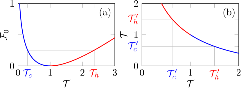
Figure 1: (a) Free-energy difference $\mathcal{F}_{0}$ at time $t=0$ for hot (red line) and cold (blue line) temperatures, $\mathcal{T}_{h}$ and $\mathcal{T}_{c}$, respectively. The $\mathcal{F}$-equidistance relation (7) is represented by the grey lines. (b) $\mathcal{T}_{h}(\mathcal{T}_{c})$ (red line) and $\mathcal{T}_{c}(\mathcal{T}_{h})$ (blue line) for $\sigma=0$, Eqs. (10). The grey lines and coloured labels indicate a temperature pair $(\mathcal{T}^{\prime}_{c},\mathcal{T}^{\prime}_{h})$, related by $\mathcal{F}$ equidistance.

Here, $W_{n}(x)$, $n=-1,0$ denotes Lambert (or product-log) function DLMF . Figure 1(b) shows $\mathcal{T}_{h}(\mathcal{T}_{c})$ (red line) and $\mathcal{T}_{c}(\mathcal{T}_{h})$ (blue line) from Eqs. (10). For $\sigma\neq 0$ the implicit condition (7) must to be inverted numerically but the curves remain almost unchanged (not shown).

After preparing the hot and cold systems at $\mathcal{F}$-equidistant temperatures, both systems are put in contact with the same heat bath with $\mathcal{T}_{f}=1$. At finite time $t>0$, the probability densities $p_{i}(x,t)$ that enter $\mathcal{F}_{i}(t)$ and thus $\mathcal{R}(t)$ are obtained from the Fokker-Planck equation by

$$p_{i}(x,t)=e^{\mathcal{L}t}p_{i}(x,0)\,.$$ (11)

In other words, in order to compute $\mathcal{R}(t)$ we must evaluate the operator exponential in Eq. (11). This can be done in the short- and long-time limits, leading to precise asymptotic results for $\mathcal{R}(t)$. As we show below, the asymptotics of $\mathcal{R}(t)$ provide an excellent characterisation of the dynamics, also at finite $t$.

For short times $t\ll 1$, the logarithmic ratio (2) reads

$$\mathcal{R}(t)\sim\mathcal{\dot{R}}(0)t=\frac{\mathcal{\dot{F}}_{h}(0)-\mathcal{\dot{F}}_{c}(0)}{\mathcal{F}_{0}}t\,,$$ (12)

where the dot denotes a time derivative and $\mathcal{F}_{0}$ is the initial free-energy difference given in Eq. (8). Through $\mathcal{\dot{F}}_{i}(0)=\int_{-\infty}^{\infty}\!\!\text{d}x\partial_{t}\,p_{i}(x,0)\ln[p_{i}(x,0)/p_{f}(x)]$, the short-time evaluation of $\mathcal{R}(t)$ depends on the time derivative $\partial_{t}p(x,0)$, evaluated at $t=0$. By expanding the exponential in Eq. (11) for $t\ll 1$, we obtain $\partial_{t}p_{i}(x,0)=(1-\mathcal{T}_{i})\partial_{x}^{2}p_{i}(x,0)$, leading us, after integration by parts, to the following integral expression for $\mathcal{\dot{F}}_{i}(0)$:

$$\mathcal{\dot{F}}_{i}(0)=-\frac{(1-\mathcal{T}_{i})^{2}}{\mathcal{T}_{i}}\int_{-\infty}^{\infty}\text{d}x\,p_{i}(x,0)V^{\prime\prime}(x)\,.$$ (13)

Evaluating Eqs. (13) and (8) for $i=h,c$, we obtain $\mathcal{R}(t)$ in the short-time limit; see Eq. (12). For $\sigma=0$ we solve Eq. (13) explicitly, which gives

$$\mathcal{\dot{F}}_{i}(0)=(1-\alpha)\frac{(\mathcal{T}_{i}-1)^{2}}{\mathcal{T}_{i}^{2/\alpha}}\frac{\Gamma(1-1/\alpha)}{\Gamma(1+1/\alpha)}\,,$$ (14)

where $\Gamma(x)$ denotes the gamma function DLMF . According to Eq. (12), whether the hot or the cold system relaxes faster at short times is determined by the sign of $\mathcal{\dot{R}}(0)$. As a function of $\alpha$ and $\mathcal{T}_{h}$, where $\mathcal{T}_{c}$ follows from $\mathcal{F}$ equidistance, it is therefore instructive to draw a “phase diagram,” marking the different regions in parameter space of initially faster heating [$\mathcal{\dot{R}}(0)>0$] and initially faster cooling [$\mathcal{\dot{R}}(0)<0$].

Figure 2(a) shows the short-time phase diagram for $\sigma=0$, spanned by $\mathcal{T}_{h}$ and $\alpha$. It separates into an upper and a lower part with different short-time behaviours. In the lower part, $\mathcal{\dot{R}}(0)>0$ so that $\mathcal{R}(t)$ is initially positive for all pairs $\mathcal{T}_{i}$; heating is faster than cooling. In the upper part, cooling is initially faster than heating. The two parts are separated by a critical line (red, dash-dotted line) where $\mathcal{\dot{R}}(0)=0$ so that $\mathcal{R}(t)$ vanishes to first order in time, $\mathcal{R}(t)\sim\mathcal{O}(t^{2})$. For $\sigma=0$, the critical line is obtained by equating $\mathcal{\dot{F}}_{c}(0)=\mathcal{\dot{F}}_{h}(0)$, and solving for $\alpha$. The smallest critical $\alpha$ value is found to be $\alpha=3$, approached for infinitesimal temperature quenches, $\mathcal{T}_{i}\to 1$. We note that this value, and the location of the critical line in general, depends on the choice of temperature measure $\mathcal{F}$. However, the existence of the critical line is robust against moderate changes of $\mathcal{F}$; see Sec. II of the SM SM .

Similarly, small variations of $\sigma$ away from zero leave the the topology of the short-time phase diagram unchanged. The generic effect of $\sigma>0$ on the critical line is shown by the green, dashed lines and black arrows in Fig. 2(a), for values of $\sigma$ up to unity. We observe that slightly increasing $\sigma$ moves the critical line to higher values but does not change the phase diagram qualitatively.

When $\sigma$ is decreased to negative values, a more complex behaviour emerges, shown by the blue, dotted lines and white arrows in Fig. 2(a): For initial temperatures close to equilibrium $\mathcal{T}_{i}\approx 1$, the critical line decreases slightly, to $\alpha$ values below $3$. For quenches far from equilibrium, on the other hand, the critical line shifts to higher $\alpha$.

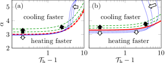
Figure 2: Relaxation-speed phase diagram for short and long times. (a) Short-time phase diagram, calculated from Eq. (13). Critical line for $\sigma=0$ (dash-dotted line), $\sigma=0.5$ and $1$ (dashed lines), and $\sigma=-0.1$, $-0.15$, and $-0.2$ (dotted lines). The black and white arrows indicate how the critical line changes as $\sigma$ is increased and decreased, respectively, from zero. (b) Long-time phase diagram, calculated using the eigenvalue decomposition (17). Critical line for $\sigma=0$ (solid line), $\sigma=0.2$ and $0.4$ (dashed lines), and $\sigma=-0.1$, $-0.15$, and $-0.2$ (dotted lines). As in Fig. 2(a), the black and white arrows indicate how the critical line changes.

We now turn to the analysis of the long-time limit $t\gg 1$ which requires different methods. When the spectrum of $\mathcal{L}$ is discrete, the relaxation of the probability densities $p_{i}$ to $p_{f}$ is exponential in the long-time limit. As a result, the densities $p_{i}$ are determined by the leading right eigenfunctions of $\mathcal{L}$ and their corresponding eigenvalues Lu and Raz (2017), obtained from the non-Hermitian eigenvalue problem

$$\mathcal{L}r_{\mu}=\lambda_{\mu}r_{\mu}\,,\qquad\mathcal{L}^{\dagger}l_{\mu}=\lambda_{\mu}l_{\mu}\,,$$ (15)

where $l_{\mu}$ and $r_{\mu}$ are the left and right eigenfunctions, respectively, and $\lambda_{\mu}$ with $\lambda_{0}=0>\lambda_{1}>\lambda_{2}>\ldots$ are the associated eigenvalues. Note that the right eigenfunction $r_{0}$ with eigenvalue $\lambda_{0}=0$ is given by the steady-state distribution $r_{0}=p_{f}$ and $l_{0}=1$. The eigenfunctions form a complete biorthogonal basis with orthonormality relations

$$\langle l_{\mu}|r_{\nu}\rangle=\int_{-\infty}^{\infty}\!\!\text{d}x\,l_{\mu}(x)r_{\nu}(x)=\delta_{\mu\nu}\,.$$ (16)

Expanding $p_{i}$ in Eq. (11) in the right eigenbasis of $\mathcal{L}$ we obtain in the long-time limit $t\gg 1$,

$$p_{i}(x,t)\sim p_{f}(x)+c_{i,\mu}e^{\lambda_{\mu}t}r_{\mu}(x)\,,$$ (17)

where $\mu$ is the lowest number for which $c_{i,\mu}\equiv\langle l_{\mu}|p_{i}(0)\rangle\neq 0$. Because our problem is symmetric with respect to the parity operation $x\to-x$, $c_{i,1}$ vanishes, so that $\mu=2$; see Sec. III in the SM SM for the case of a harmonic potential. All higher-order terms in Eq. (17) that play a role at finite times are exponentially suppressed in the long-time limit considered here. Using Eqs. (2) and (17) we find that $\mathcal{R}(t)$ approaches a constant $\mathcal{R}_{\infty}$ for $t\gg 1$ that depends only on the coefficients $c_{i,2}$:

$$\mathcal{R}(t)\sim 2\ln\left(\left|\frac{c_{h,2}}{c_{c,2}}\right|\right)\equiv\mathcal{R}_{\infty}\,.$$ (18)

Hence, the relative magnitude of the free-energy differences is determined by the initial overlap between the left eigenvector $l_{2}$ of $\mathcal{L}$ and the initial distributions $p_{i}(x,0)$ before the temperature quench Lu and Raz (2017).

We determine $c_{i,2}$ by solving the eigenvalue problem (15) numerically, discretising it on an evenly spaced, finite lattice with small lattice spacing. Equations (15) then become matrix eigenvalue problems involving large, non-symmetric matrices, whose left and right eigenvectors are approximations of the left and right eigenfunctions $r_{\mu}$ and $l_{\mu}$.

Figure 2(b) shows the long-time phase diagram for $\sigma=0$ obtained from numerically computing $c_{i,2}$ and evaluating $\mathcal{R}_{\infty}$ in Eq. (18). The general structure of the long-time phase diagram is qualitatively similar to that of the short-time phase diagram in Fig. 2(a), featuring regions of faster heating ($\mathcal{R}_{\infty}>0$) and faster cooling ($\mathcal{R}_{\infty}<0$). For long times, however, the critical line [solid line in Fig. 2(b)] is located at slightly higher values. Consequently, the minimum of the critical line, attained for close-to-equilibrium quenches, takes the slightly larger value $\alpha\approx 3.31$. As in the short-time limit, the long-time critical line is only weakly perturbed by moderate changes of the temperature measure $\mathcal{F}$; see Sec. II of the SM SM for details.

Upon increasing $\sigma$, we again observe no qualitative change of the phase diagram; the critical line is merely pushed to larger $\alpha$ values [green, dashed lines in Fig. 2(b)]. Negative $\sigma$, on the other hand, leads to a qualitative change: For $\sigma<0$, the region of asymptotically faster cooling becomes finite and is completely enclosed by the critical line [blue, dotted lines in Fig. 2(b)]. The sensitive dependence of the relaxation dynamics on negative values of $\sigma$, observed both in the short- and long-time limits, must be due to the emergence of bistability of the potential $V(x)$, Eq. (4). The existence of two potential minima gives rise to multiple relaxation timescales associated with the relaxation within the same minimum and across the two minima.

From the general structure of the phase diagrams we conclude that asymptotically steep potentials (large $\alpha$) lead to faster cooling, compared to $\mathcal{F}$-equidistant heating, when the initial temperature differences are not too large. For small $\alpha$, the opposite is true. Intuitively, this may be explained by noting that for an initially hot system, more probability is located in the tails of the distribution. The steeper the potential, the faster this tail probability is advectively transported toward the potential minimum, leading to faster cooling. For small $\alpha$, this advection effect is weaker, so that it is outperformed by the diffusive broadening of the bulk of the distribution of the cold system, thus resulting in faster heating.

Our analysis reveals the existence of distinct critical lines in the short- and long-time limits. This results in an overlap between the faster-heating and faster-cooling regions at short and long times, giving rise to a crossover region in the phase diagram. In the crossover region, the hot system initially relaxes faster [$\mathcal{R}(t)<0$], but is eventually overtaken by the initially colder system [$\mathcal{R}(t)>0$]. Hence, there must be at least one finite time $t_{c}>0$ where $\mathcal{R}(t_{c})=0$, i.e., the system crosses over from faster cooling to faster heating.

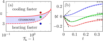
Figure 3: (a) Superimposed short- and long-time phase diagrams for $\sigma=0$, featuring the critical lines in the short-time (dash-dotted line) and long-time (solid line) limits. The crossover region is shown by the cross-hatched region. The coloured dots correspond to the parameter values for the plots in Fig. 3(b). (b) $\mathcal{R}(t)$ from different numerical methods for $\mathcal{T}_{h}=3$ and $\alpha=3$, $3.3$ and $3.5$, in blue, green and red, respectively. The dash-dotted lines show results obtained from Eq. (11), by numerically calculating the spectrum of $\mathcal{L}$. The solid lines are computed from numerical simulations of the Langevin equation. The black, dashed lines correspond to the short- and long-time asymptotics.

Figure 3(a) shows the superimposed short- and long-time phase diagrams for $\sigma=0$ featuring the crossover region (cross-hatched area). The dash-dotted and solid lines show the critical lines from Figs. 2(a) and (b), respectively.

In order to study the behaviour of $\mathcal{R}(t)$ in the crossover region, and to validate our previous results, we perform a numerical analysis of the finite-time evolution of $\mathcal{R}(t)$. We focus on a few points in the phase diagram, shown as the differently coloured dots in Fig. 3(a), where we expect qualitatively different behaviours: For the parameter sets represented by the blue and red dots, we expect heating and cooling, respectively, to be faster, both for short and for long times. By contrast, for the parameters of the green dot we expect at least one finite-time crossover from faster cooling to faster heating.

For the finite-time analysis we use two different numerical methods. First, we obtain an approximation of $p_{i}(x,t)$ by using the discretised analogue of Eq. (11) obtained with the discretisation scheme discussed earlier.

The second method approximates the probability density $p_{i}(x,t)$ by means of a Langevin approach Van Kampen (1992): We simulate a large number of trajectories $x_{i}(t)$, $i=h,c$, following the dynamics $\dot{x}_{i}(t)=-V^{\prime}(x)+\xi(t)$, where $\xi(t)$ is a Gaussian white-noise signal with correlation function $\langle\xi(t)\xi(t^{\prime})\rangle=2\delta(t-t^{\prime})$. The initial values $x_{i}(0)$ are sampled from the equilibrium distributions $p_{i}(x,0)$ prior to the temperature quench. The Langevin equation is solved numerically using an Euler-Maruyama scheme Kloeden and Platen (1992) with a small time step. The probability densities $p_{i}(x,t)$ are then computed by generating histograms over all locations $x_{i}(t)$ at discrete times $t$.

These methods, whose parameters are summarised in Sec. IV of the SM SM , yield two independent numerical approximations $p_{i}(x,t)$ from which we then calculate $\mathcal{R}(t)$. Figure 3(b) shows the so-obtained $\mathcal{R}(t)$, where the colours of the curves correspond to the colours of the dots in Fig. 3(a). The dash-dotted lines show $\mathcal{R}(t)$ calculated from the discretised operator $\mathcal{L}$. The lighter, solid lines show the corresponding results from the Langevin approach. Also shown are the short- and long-time asymptotes (dashed lines). We observe that the asymptotes represent a good characterisation of the dynamics of $\mathcal{R}(t)$ for all times. In particular, there are no finite-time crossings $\mathcal{R}(t_{c})=0$ for the parameter values outside of the crossover region in Fig. 3(a), i.e., for the blue and red curves. Inside the crossover region [see green curve in Fig. 3(b)] we observe only a single crossing.

Furthermore, there is good agreement between the results from the different numerical methods and the asymptotic results. Note that the deviations between the equally coloured curves become larger for longer times. The reason is that for long times, the individual free-energy differences $\mathcal{F}_{i}(t)$ in Eq. (2) become exponentially small, so that the relative errors increase as $t$ becomes large. Due to this numerical difficulty, we were unable to evaluate $\mathcal{R}(t)$ until convergence, as can be seen by the discrepancy between our numerical results and the long-time asymptotics [horizontal, dashed lines in Fig. 3(b)].

Finally, we note that far from equilibrium, for $\mathcal{T}_{c}\approx 0.0229$ and $\mathcal{T}_{h}\approx 5.50$, the short- and long-time critical lines cross [see Fig. 3(a)] which implies the existence of an inverted crossover region very far from equilibrium where heating is initially faster but asymptotically slower than cooling.

In conclusion, $\mathcal{F}$-equidistant thermal relaxation of overdamped diffusions in anharmonic potentials $V(x)$ allows for both faster heating and faster cooling, even when $V(x)$ has a single minimum. As a consequence, the short- and long-time phase diagrams [Figs. 2(a) and (b)], spanned by the $(\mathcal{T}_{h},\alpha)$-parameter space, are nontrivial, exhibiting regions of faster heating and faster cooling. Both for short and for long times, we found that cooling is faster than heating for sufficiently large $\alpha$, and heating is faster than cooling for small $\alpha$. This can be explained in terms of a competition between the advective relaxation of the tail probability of the hot system, and the diffusive broadening of the bulk-probability in the cold system. Despite the similarities between the short- and long-time phase diagrams, we found that their critical lines are different, and that the faster-heating and faster-cooling regions overlap. Superimposing the two, we localised a crossover region [Fig. 3(a)] where cooling is initially faster but the rate of heating eventually overtakes. Outside of the crossover region, we found no crossings, suggesting that the short- and long-time asymptotics faithfully characterise the relative relaxation speeds. The critical lines separating the parameter regions with different behaviours are only weakly perturbed by moderate changes of the temperature measure $\mathcal{F}$ or by an additional harmonic term in the potential $V(x)$, as long as the latter remains single-well, i.e., $\sigma>0$.

It would be interesting to test the relaxation-speed crossover in experiments and thus to reproduce our phase diagram under experimental conditions. This requires tracking the changes in energy and entropy of the system throughout the experiment which is possible in state-of-the-art setups Kumar and Bechhoefer (2020); Ciliberto (2017). On the theoretical side, it would be desirable to understand the precise dynamical origin of the different relaxation behaviours . This might lead to optimisation methods for the potential to achieve faster heating or cooling, perhaps in the spirit of first-passage time optimisation Palyulin and Metzler (2012); Chupeau et al. (2020).