A Penalized Shared-parameter Algorithm for Estimating Optimal Dynamic Treatment Regimens

Abstract

[Abstract]A dynamic treatment regimen (DTR) is a set of decision rules to personalize treatments for an individual using their medical history. The Q-learning based Q-shared algorithm has been used to develop DTRs that involve decision rules shared across multiple stages of intervention. We show that the existing Q-shared algorithm can suffer from non-convergence due to the use of linear models in the Q-learning setup, and identify the condition in which Q-shared fails. Leveraging properties from expansion-constrained ordinary least-squares, we give a penalized Q-shared algorithm that not only converges in settings that violate the condition, but can outperform the original Q-shared algorithm even when the condition is satisfied. We give evidence for the proposed method in a real-world application and several synthetic simulations.

1 Introduction

A dynamic treatment regimen (DTR) refers to a set of decision rules for developing personalized multistage treatment using the patient’s covariate and treatment history ¹³, ¹⁶, ⁵, ⁹. At each stage of the disease, a DTR can recommend the best treatment for an individual based on their medical history up to that time. In recent times, DTRs have been used in various domains of medical and social sciences to leverage the data-driven personalized medicine; for example, in mental health ¹⁵, ⁷, ¹⁹, cancer ²³, ¹¹, autism ¹, weight loss ², education ²² and others.

In dynamic treatment regimens, a shared decision rule is a common function of the time-varying covariate(s) across stages. For instance, a patient suffering from depression is medicated when the depression score (e.g., Quick Inventory of Depressive Symptomatology (QIDS)) crosses a threshold independent of the duration of diagnosis or treatment ¹⁸. In HIV patients, Interleukin 7 (IL-7) injections are given when the CD4 count falls below a threshold ²¹. Treatments are given to diabetic patients when the HbA1c (Hemoglobin A1c) crosses a threshold ⁶. Note that in all the three examples, a treatment or intervention is offered based on a specific threshold which does not change over time or stages of diseases. This means the decision rule to offer a treatment is shared across different stages.

The Q-shared algorithm, proposed by ³, is a Q-learning-based procedure for estimating shared-parameter DTRs, where the Q-function is modelled via linear regression. Some of the parameters in the stage-specific linear regression models remain the same across the stages to capture the sharing property of the decision rules. However, ¹⁶ in his work on simultaneous g-estimation, and ³ pointed out that the use of a linear model may lead to the failure of the convergence of the estimated parameters to their true values. This drawback of the Q-shared algorithm can limit its use. We explore the issue of the non-convergence under the Q-shared setup and find examples when the Q-shared method fails. Finally, we propose a shrinkage based penalized Q-shared algorithm that avoids the non-convergence issue. ²⁰ previously used shrinkage methods in Q-learning. However, that was in the context of unshared Q-learning. Recently, ²⁴ proposed two methods called the censored shared-Q-learning and the censored shared-O-learning for censored data. But, their approaches are not based on shrinkage methods, even though they mentioned the lasso penalty.

In this work, our main contributions are: a) to demonstrate at least two instances where linear models, as Q-functions in the Q-shared algorithm, fail to converge; and, b) to propose a penalized Q-shared algorithm that avoids the non-convergence problem and gives better treatment allocation matching compared to the original Q-shared algorithm. Therefore, penalized Q-shared algorithm is a better option compared to Q-shared, irrespective of the non-convergence issue. The proposed algorithm can be easily implemented in a shared-parameter estimation problem.

2 Optimal DTR with Shared Parameter: Q-shared Algorithm

Let us consider a study with $J$ stages. In this study, longitudinal data for a patient is given as $(O_{1},A_{1},...,O_{J},A_{J},O_{J+1})$ where $O_{j}$ are the covariates measured prior to the treatment at the $j^{\text{th}}$ stage and $A_{j}$ is the treatment assigned at the $j^{\text{th}}$ stage, for $j=1,\cdots,J$. The $O_{J+1}$ denotes the end-of-study observation at the end of the $J^{th}$ stage ⁵, ³. The binary treatment options available at each stage, coded $\{t_{1},t_{2}\}$, are randomly assigned with known probabilities (e.g., even-randomization). The primary outcome is defined as a function of the patient’s history as follows $Y=g(H_{J+1})$, where $g(\cdot)$ is a real-valued function and history $H_{j}=(O_{1},A_{1},\dots,O_{j})$ for $j\ =\ 1,2,\dots,J+1$. The objective functions, also known as Q-functions ¹⁴, are given by

$$Q_{J}(H_{J},A_{J}) = \mathbb{E}[Y|H_{J},A_{J}]$$

$$Q_{j}(H_{j},A_{j}) = \mathbb{E}[\max_{a_{j+1}}Q_{j+1}(H_{j+1},A_{j+1})|H_{j},A_{j}]\text{ for }j=J-1,\dots,1$$

The optimal DTR is $d_{j}(h_{j})=arg\ max_{a_{j}}\ Q_{j}(h_{j},a_{j})$. The Q-functions can be estimated by linear regression as $Q_{j}(H_{j},A_{j};\beta_{j},\psi_{j})={\beta_{j}}^{T}H_{j0}+\ ({\psi_{j}}^{T}H_{j1})A_{j}$ where $H_{j0}$ is the “main effect of history” and $H_{j1}$is the “interaction effect of history”. Hence, the optimal DTR can be expressed as $d_{j}(h_{j})=arg\ max_{a_{\text{j\ }}}Q_{j}(h_{j},a_{j};\beta_{j},\psi_{j})$. An optimal DTR, defined as the vector of decision rules $(d_{1},...,d_{J})$, when estimated using standard Q-learning, is calculated by recursively moving backwards through stages. This setup can be called Q-unshared. Let us look at the Q-shared algorithm where the decision rule parameters are shared across different stages ³. Here, we have $\psi_{1}=\dots=\psi_{J}=\psi$. The Q-functions can be estimated as

$$Q_{j}(H_{j},A_{j})=\mathbb{E}[Y_{j}(\theta_{j+1})|H_{j},A_{j}]\text{ for }j=1,2,...,J-1,$$

where ${\theta_{j}}^{T}=({\beta_{j}}^{T},{\psi^{T}})$, $\beta_{j}$s are unshared parameters while $\psi$ is the shared parameter, and

$$Y_{j}(\theta_{j+1})={\beta^{T}_{j+1}}H_{j+1,0}+\max\{t_{1}\times{\psi^{T}_{j+1}}H_{j+1,1},t_{2}\times{\psi^{T}_{j+1}}H_{j+1,1}\}$$

is the population-level $j^{\text{th}}$ stage pseudo-outcome. For $\{t_{1},t_{2}\}=\{-1,1\}$, $\max\{t_{1}\times{\psi^{T}_{j+1}}H_{j+1,1},t_{2}\times{\psi^{T}_{j+1}}H_{j+1,1}\}=|\psi^{T}_{j+1}H_{j+1,1}|$. The Q-function for the $J^{th}$ stage remains the same. $J$ regression equations can be written as $Q_{j}=\mathbf{Z}_{j}\theta_{j}$ for $j\ =\ 1,\dots,J$ where $\mathbf{Z}_{j}=({H_{j0}}^{T},{H_{j1}}^{T}A_{j})$ and ${\theta_{j}}^{T}=({\beta_{j}}^{T},{\psi^{T}})$. Combining data from J stages, we get,

$$\begin{pmatrix}Y\\ Y_{J-1}(\theta_{J})\\ \vdots\\ Y_{1}(\theta_{2})\\ \ \end{pmatrix}\ =\ \begin{pmatrix}\mathbf{Z}_{J}^{(\beta_{J})}&\mathbf{0}&\cdots&\mathbf{0}&\mathbf{Z}_{J}^{\psi}\\ \mathbf{0}&\mathbf{Z}_{J-1}^{\beta_{J-1}}&\cdots&\mathbf{0}&\mathbf{Z}_{J-1}^{\psi}\\ \vdots&\vdots&&\vdots&\vdots\\ \mathbf{0}&\mathbf{0}&\cdots&\mathbf{Z}_{1}^{\beta_{1}}&\mathbf{Z}_{1}^{\psi}\end{pmatrix}\times\begin{pmatrix}\beta_{J}\\ \beta_{J-1}\\ \vdots\\ \beta_{1}\\ \psi\end{pmatrix}+\varepsilon$$

which can be written as $Y^{*}(\theta)=\mathbf{Z}\theta+\varepsilon$ with $\theta^{T}=({\beta_{J}}^{T},...,{\beta_{1}}^{T},\psi^{T})$ and $\varepsilon$ as the error term. To estimate $\theta$, we wish to minimize

$$J(\theta)\ =\ ||Y^{*}(\theta)-\mathbf{Z}\theta||^{2}.$$

This poses a problem because $Y^{*}(\theta)$ involves the unknown $\theta$ term that includes shared parameters. In the absence of closed-form solution, ³ proposed an iterative Q-shared algorithm by using the Bellman residual, $Y^{*}(\theta)-\mathbf{Z}\theta$, instead of directly minimizing $J(\theta)$. They took the score function as $S_{\theta}(\mathbf{Z})=\frac{\partial}{\partial\theta\ }((\mathbf{Z}\theta)^{T})=\mathbf{Z}^{T}$, and formulated the estimating equation as $S_{\theta}(\mathbf{Z})\ \times(Y^{*}(\theta)-\mathbf{Z}\theta)\ =0$. The algorithm 1 describes the steps to estimate parameters using the Q-shared algorithm.

Algorithm 1 Q-shared algorithm:

1. Set starting value of $\theta$ (one can estimate from data, or guess); define it as ${\hat{\theta}}^{(0)^{T}}=({{\hat{\beta}}_{J}}^{(0)^{T}},\dots,{{\hat{\beta}}_{1}}^{(0)^{T}},{\hat{\psi}}^{(0)^{T}})$

2. For $k=0,1,2,\dots$, at the $(k+1)^{\text{th}}$ iteration:

   1. Formulate the vector $Y^{*}({\widehat{\theta}}^{(k)})$.

   2. To obtain ${\hat{\theta}}^{(k+1)}$, solve the estimating equation $\mathbf{Z}^{T}(Y^{*}({\hat{\theta}}^{(k)})-\mathbf{Z}{\theta})=0$ for $\theta$.

3. Repeat (2a) and (2b) until convergence. Specifically, for a prespecified value of $\varepsilon$ and for some $k$, continue till $||{\hat{\theta}}^{(k+1)}-{\hat{\theta}}^{(k)}||<\varepsilon$.

3 Non-convergence of Q-shared algorithm

The Q-shared algorithm shares similarities with the ubiquitous least squares regression, and we can better ground our understanding of Q-shared through the intuition of least squares. The ordinary least squares estimate for the model $Y\sim{\mathbf{X}}\beta$, is $\hat{\beta}=arg\min_{\beta}||{\mathbf{X}}\beta\ -\ Y||_{2}=({\mathbf{X}}^{T}\mathbf{X})^{-1}{\mathbf{X}}^{T}Y$. Let $\hat{Y}$ be the predicted value for $Y$, then $\hat{Y}={\mathbf{X}}\widehat{\beta}={\mathbf{X}}({\mathbf{X}}^{T}{\mathbf{X}})^{-1}{\mathbf{X}}^{T}Y=\mathbf{H}Y$, where $\mathbf{H}$ is the hat matrix. Assuming $({\mathbf{X}}^{T}{\mathbf{X}})^{-1}$ exists (and thus implying $\mathbf{H}$ exists) and based on the discussion by ¹², we can say that Q-shared may fail when the corresponding hat matrix $\mathbf{H}$ is not an $\infty$-norm non-expansion. Note that $\mathbf{H}$ will be $\infty$-norm non-expansion if

$$||\mathbf{H}||_{op(\infty)}=\text{max}_{i}{\ \Sigma_{j}\ |\mathbf{H}}_{\text{ij}}|\ \leq 1,$$ (1)

where $\mathbf{H}_{\text{ij}}$ is the $(i,j)^{\text{th}}$ element of the hat matrix $\mathbf{H}$. Therefore, the convergence of the Q-shared algorithm is not guaranteed during the estimation of parameters if (1) is violated. ¹⁶ also discussed the non-convergence due to the use of linear models in the context of simultaneous g-estimation. We show two examples where the above Q-shared algorithm fails to converge, indicating a limitation of its applicability.

Consider a three-stage ($J=3$) SMART design where responders enter the follow-up phase and exit the study and non-responders are re-randomized again in the next stage. We use a simulated data set given in ³ to show that the Q-shared algorithm fails to converge after a slight modification in the covariates in the same data. The first few rows of the data is given in Table 1, where $Y_{1},Y_{2}$ and $Y_{3}$ are intermediate stage-specific outcomes corresponding to stages 1, 2 and 3, respectively. The primary outcome is defined as $Y_{Primary}=R_{1}Y_{1}+(1-R_{1})R_{2}((Y_{1}+Y_{2})/2)+(1-R_{1})(1-R_{2})((Y_{1}+Y_{2}+Y_{3})/3)$, where $R_{1}$ and $R_{2}$ are responder indicators corresponding to stages 1 and 2, respectively (0: non-responder and 1: responder). The stage specific treatments $A_{j},j=1,2,3$ and covariates $O_{j},j=1,2,3$ are all binary, coded $\{-1,1\}$. The total sample size (number of rows) of the data is 300. To apply the Q-shared algorithm, we consider the initial estimates of all the parameters as zeros, i.e., ${{\hat{\theta}}}^{(0)}=({{\hat{\beta}}_{J}}^{(0)^{T}},...,{{\hat{\beta}}_{1}}^{(0)^{T}},{\hat{\psi}}^{(0)^{T}})=(0^{T},{...,0}^{T},0^{T})$. Note that, in the Q-shared algorithm, for a specific iteration ($Y^{*}(\theta)$ is known), $X=Z$. In the above data, the Q-shared algorithm converged in 8 iterations. However, we observed that the corresponding $H$ matrix is not an $\infty$-norm non-expansion using (1). We see the norm of Hat ($\mathbf{H}$) matrix as $||\mathbf{H}||_{op(\infty)}=||\mathbf{X}({\mathbf{X}}^{T}{\mathbf{X}})^{-1}{\mathbf{X}}^{T}||_{op(\infty)}=4.52$. The estimated parameters, along with $m$-out-of-$n$ bootstrap variances and 95% confidence interval (CI), are presented in Table 2. Note that, we have used the $m$-out-of-$n$ bootstrap to restore bootstrap consistency in the presence of non-regularity ⁴, ³.

Table 1: First few rows of the data set used by ³.

	$Y_{1}$	$Y_{2}$	$Y_{3}$	$Y_{Primary}$	$A_{1}$	$A_{2}$	$A_{3}$	$O_{1}$	$O_{2}$	$O_{3}$	$R_{1}$	$R_{2}$
1	1.5448	2.857	2.230	1.544	-1	-1	-1	-1	-1	-1	1	1
2	-0.4734	-0.688	-0.724	-0.580	1	1	1	1	1	1	0	1
3	0.4853	-0.327	-0.741	0.485	1	1	-1	-1	-1	1	1	1
4	-0.4224	0.547	-0.377	-0.084	1	-1	1	-1	1	-1	0	0
:	:	:	:	:	:	:	:	:	:	:	:	:

Table 2: Estimated parameters using Q-shared algorithm.

		Using $m$-out-of-$n$ bootstrap
Shared Parameter	Estimate	Variance	CI
$\psi_{0}$	-0.0974	0.0061	(-0.2156, 0.1040)
$\psi_{1}$	0.0802	0.0024	(-0.0192, 0.1710)
$\psi_{2}$	0.0876	0.0055	(-0.0522, 0.2366)
$\psi_{3}$	-0.0409	0.0101	(-0.2365, 0.1616)

Example 1:

In the above simulated example, the binary treatment $A_{i}$ is coded as $\{-1,1\}$. However, there is no specific reason behind it except for easy calculation. Now, we code the binary $A_{i}$ in the same data as $\{-0.1,0.1\}$ in place of $\{-1,1\}$, respectively. In this modified data, we applied the Q-shared algorithm and observed that it fails to converge to one particular value in most of the 1000 $m$-out-of-$n$ bootstrap replications. From different iterations, we notice that most of the iterations converge to different values, which result in the high variances of parameter estimates as shown in the table. We notice that $||\mathbf{H}||_{op(\infty)}=||\mathbf{X}({\mathbf{X}}^{T}{\mathbf{X}})^{-1}{\mathbf{X}}^{T}||_{op(\infty)}=4.52$ is greater than 1, and hence convergence is not guaranteed, which we observe in our case. Table 3 shows the estimated parameters along with $m$-out-of-$n$ bootstrap variances and 95% confidence interval (CI). Such high variances, for the last two parameters in Table 3, are not useful. They do not provide information about the precise value of the estimates, and hence we need alternative methods to solve the problem with this particular setting.

Table 3: Example 1: Estimated parameters using Q-shared algorithm from modified data.

		Using $m$-out-of-$n$ bootstrap
Shared Parameter	Estimate	Variance	CI
$\psi_{0}$	-0.98	0.64	(-2.13, 0.95)
$\psi_{1}$	0.80	0.23	(-0.24, 1.59)
$\psi_{2}$	8.75	39.99	(-4.28, 19.76)
$\psi_{3}$	-41.04	10652.00	(-196.89, 156.35)

Example 2:

We now again modify the data used in example 1 by considering $A_{1},A_{2},A_{3}\in\{0.250,0.248\}$ and $O_{1},O_{2},O_{3}\in\{-0.01,0.01\}$. The close values of $A_{i}$ could indicate two different doses of a highly sensitive medicine, and hence such a set up could be relevant in understanding how DTRs work in such a near-continuous treatment setting. Following the same procedure as in example 1, we once again notice that the shared parameters converge to different values in most of the 1000 $m$-out-of-$n$ bootstrap replications and result in a high variance, which is a sign of non-convergence. We notice that $||\mathbf{H}||_{op(\infty)}=||\mathbf{X}({\mathbf{X}}^{T}{\mathbf{X}})^{-1}{\mathbf{X}}^{T}||_{op(\infty)}=4.04$. Table 4 shows the estimated parameters along with $m$-out-of-$n$ bootstrap variances and 95% confidence interval (CI). We observe high variances for all the estimated parameters. The above two examples show that the Q-shared algorithm may not convergence always. Therefore, we need an algorithm that can address the non-convergence issue.

Table 4: Example 2: Estimated parameters using Q-shared algorithm from modified data.

		Using $m$-out-of-$n$ bootstrap
Shared Parameter	Estimate	Variance	CI
$\psi_{0}$	76.11	5155.40	(-48.54, 195.80)
$\psi_{1}$	-9012.76	17754686.40	(-15209.08, 1366.60)
$\psi_{2}$	356.14	263149.90	(-425.29, 1495.40)
$\psi_{3}$	-2997.56	4700155.70	(-7240.85, 1291.90)

4 Penalized Q-shared Algorithm

We have demonstrated that the Q-shared algorithm fails to converge in at least two concrete examples. Moreover, from the $m$-out-of-$n$ bootstrap replicates, we observe high variances for estimates of the shared parameters. It prompts us to think about shrinkage methods inside the Q-shared algorithm instead of the linear regression model to control the high variability ¹⁰. In algorithm 2, we propose the penalized Q-shared algorithm that uses ridge regression as the shrinkage method.

Algorithm 2 Penalized Q-shared algorithm:

1. Set starting value of $\theta$ (one can estimate from data, or guess); define it as ${\hat{\theta}}^{(0)^{T}}=({{\hat{\beta}}_{J}}^{(0)^{T}},\dots,{{\hat{\beta}}_{1}}^{(0)^{T}},{\hat{\psi}}^{(0)^{T}})$

2. For $k=0,1,2,\dots$, at the $(k+1)^{\text{th}}$ iteration:

   1. Formulate the vector $Y^{*}({\widehat{\theta}}^{(k)})$.

   2. Get, ${\hat{\theta}}^{(k+1)}\ =\ arg\ min{}_{\theta}(||{\mathbf{Z}}{{\theta}}-Y^{*}({\hat{\theta}}^{(k)})||_{2}+\lambda||{{\theta}}||_{2})$

3. Repeat (2a) and (2b) until convergence. Specifically, for a prespecified value of $\varepsilon$ and for some $k$, continue till $||{\hat{\theta}}^{(k+1)}-{\hat{\theta}}^{(k)}||<\varepsilon$.

Here, note that, we do not have to use an approximate estimating equation involving the Bellman residual instead of minimizing the squared Bellman error to obtain the $\hat{\theta}^{(k+1)}$. ³ used the approximate estimating equation involving the Bellman residual to avoid instability or non-convergence during the estimation process. Here, the ridge regression takes care of those issues in the form of the penalty parameter $\lambda$. The $\lambda\geq 0$ controls the extent of shrinkage. A larger value of $\lambda$ indicates a higher amount of shrinkage. The optimal value of $\lambda$ in the above algorithm (step 2(b)) can be obtained by minimizing the 10-fold cross validation error ⁸ as

$$\hat{\lambda}=\ arg\ min{}_{\lambda}\biggl{[}\frac{1}{10}\sum_{v=1}^{10}\frac{1}{n_{S_{v}}}\sum_{u\in S_{v}}(Y_{obs,u}(\lambda)-\hat{Y}_{Pred,u}(\lambda))^{2}\biggr{]},$$

where $(S_{1},S_{2},\cdots,S_{10})$ denote the 10 partitions of the data with corresponding number of subjects as $(n_{S_{1}},n_{S_{2}},\cdots,n_{S_{10}})$, respectively. $Y_{obs,u}(\lambda)$ = $Y_{u}^{*}({\hat{\theta}}^{(K)})$ and $\hat{Y}_{Pred,u}(\lambda)=\mathbf{Z}_{u}{\hat{\theta}}^{(K)}$ denote the observed and the predicted values of the primary outcome for the $u^{th}$ subject in a partition based on the final iterative stage $K$ of the penalized Q-shared algorithm, respectively. Note that $\hat{\theta}^{(K)}$ is a function of $\lambda$ and known for a given value of $\lambda$.

It is natural to also consider $L_{1}$ regularization. However, $L_{1}$ regularized regression, or the lasso ¹⁰, is generally applied for the purposes of variable selection or denoising; in the context of Q-shared, we are simply attempting to improve variability in parameter estimates at the cost of bias. This is a task best suited for $L_{2}$ regularization, and so we leave $L_{1}$ regularization to future work.

5 Simulation Studies

The objective of the following simulation study is to show that the proposed penalized Q-shared algorithm performs better than the existing Q-shared algorithm in two aspects. First, the penalized Q-shared algorithm does converge when Q-shared does not. Secondly, when there are no issues of non-convergence, the performance of the penalized Q-shared algorithm is better than the Q-shared with respect to allocating appropriate treatments to patients. In other words, there is no reason not to employ penalized Q-shared over the original Q-shared.

In section 3, we have provided two examples where the existing Q-shared algorithm fails to converge. Here, we use the penalized Q-shared algorithm for the same data used for two examples. Tables 5 and 6 show the estimated parameters along with corresponding $m$-out-of-$n$ bootstrap variances and 95% confidence interval (CI) using penalized Q-shared for the examples 1 and 2, respectively. In both examples, we have used 1000 $m$-out-of-$n$ bootstrap iterations. We can see that in both the examples, the estimated parameters have small variances. In other words, when the difference between the two values of the binary treatment is small, the Q-shared method may not give satisfactory results. It could be a significant issue in SMART when the difference between two administered doses of the same medicine is very close. In figure 1, we have shown the convergence patterns of the Q-shared and the penalized Q-shared algorithms based on 50 $m$-out-of-$n$ bootstrap samples related to example 2 for all the four parameters $\psi_{0},\psi_{1},\psi_{2}$ and $\psi_{3}$. It is evident from the top row of figure 1 that the Q-shared algorithm fails to converge and exhibits high variability for all four parameters. In contrast, the bottom row of figure 1 indicates a convergence of the penalized Q-shared algorithm with extremely low variances for all four parameters.

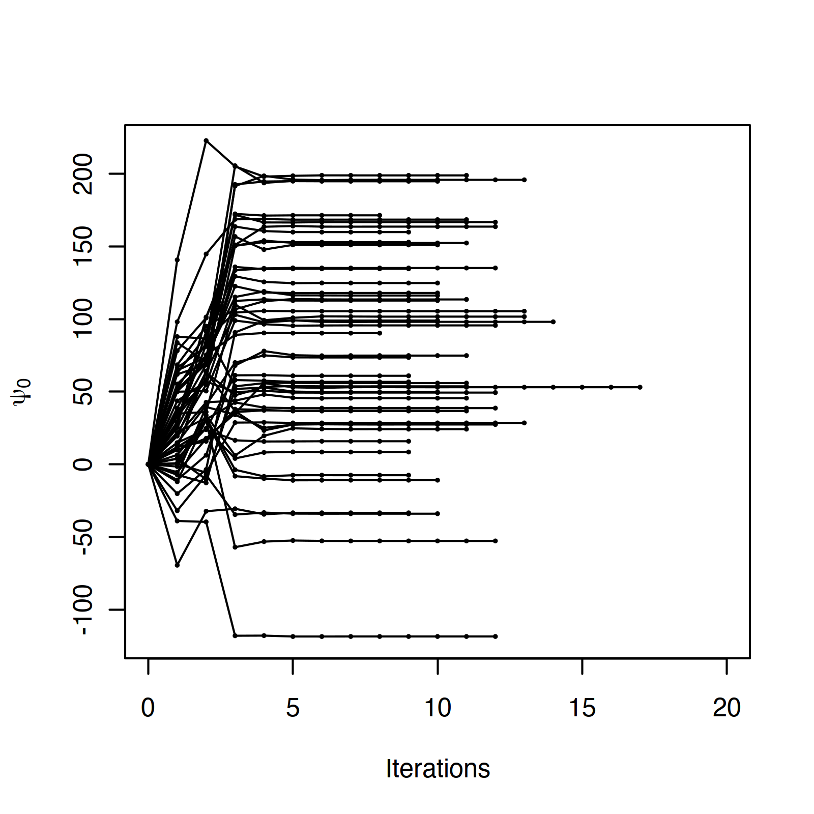
((a)) Q-shared: $\psi_{0}$

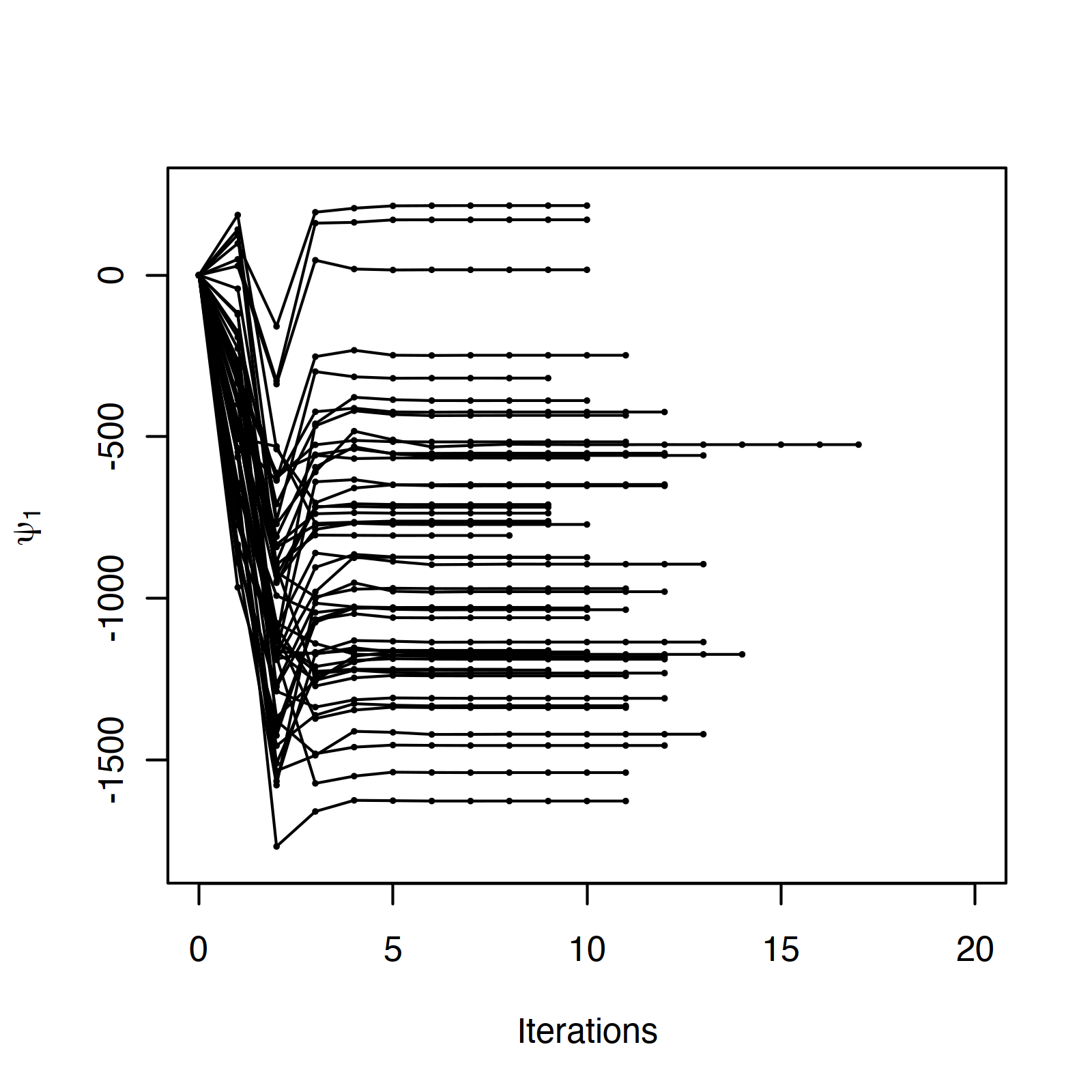
((b)) Q-shared: $\psi_{1}$

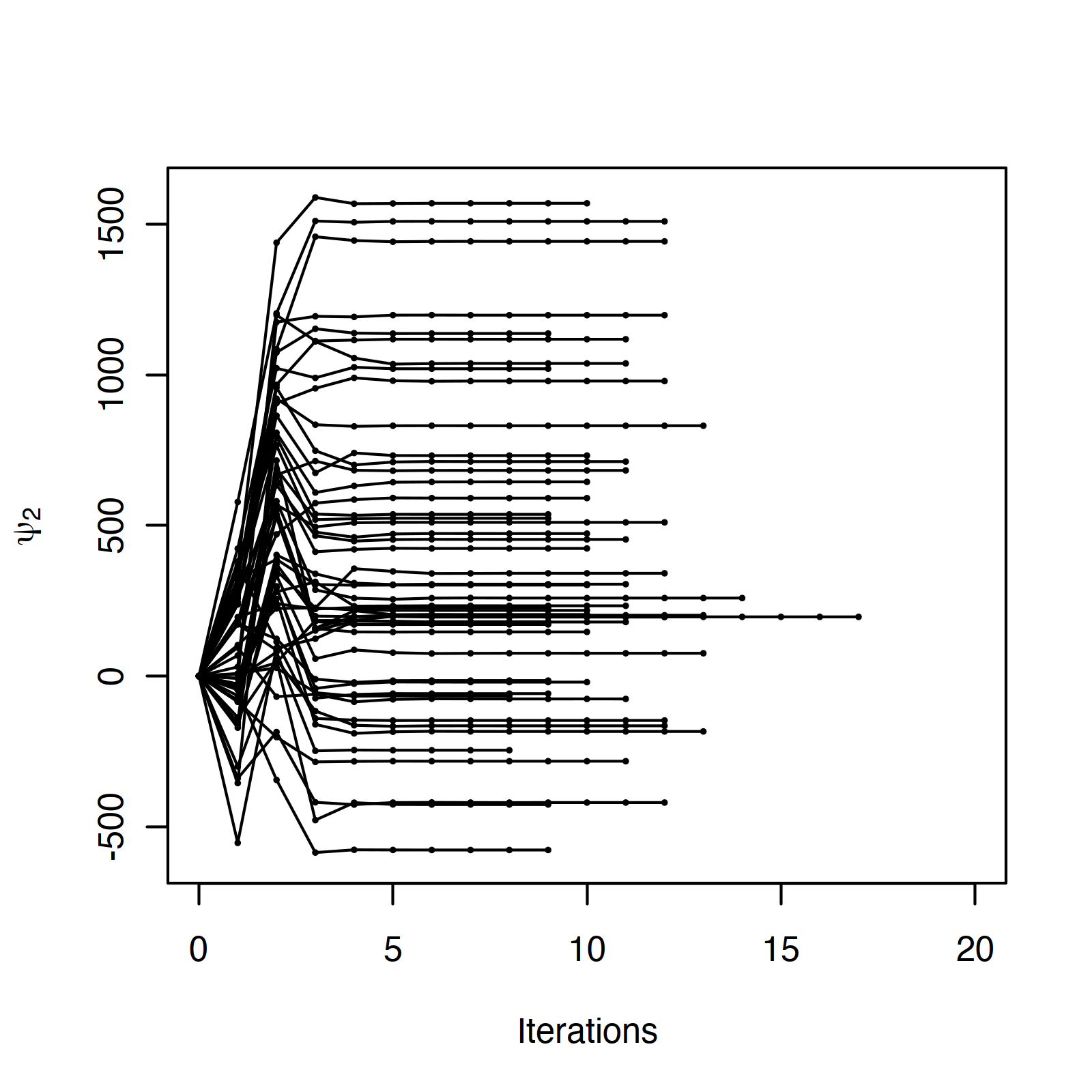
((c)) Q-shared: $\psi_{2}$

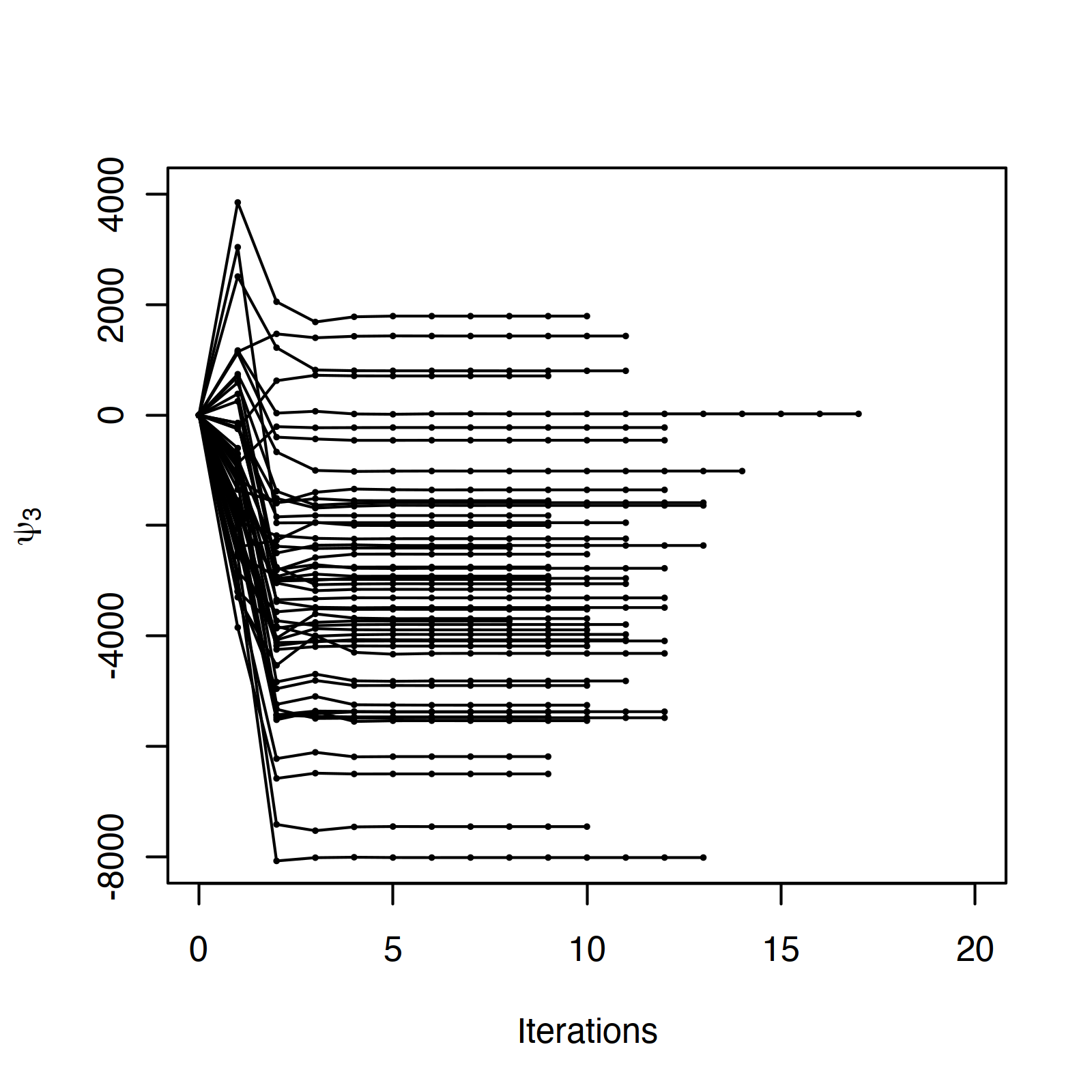
((d)) Q-shared: $\psi_{3}$

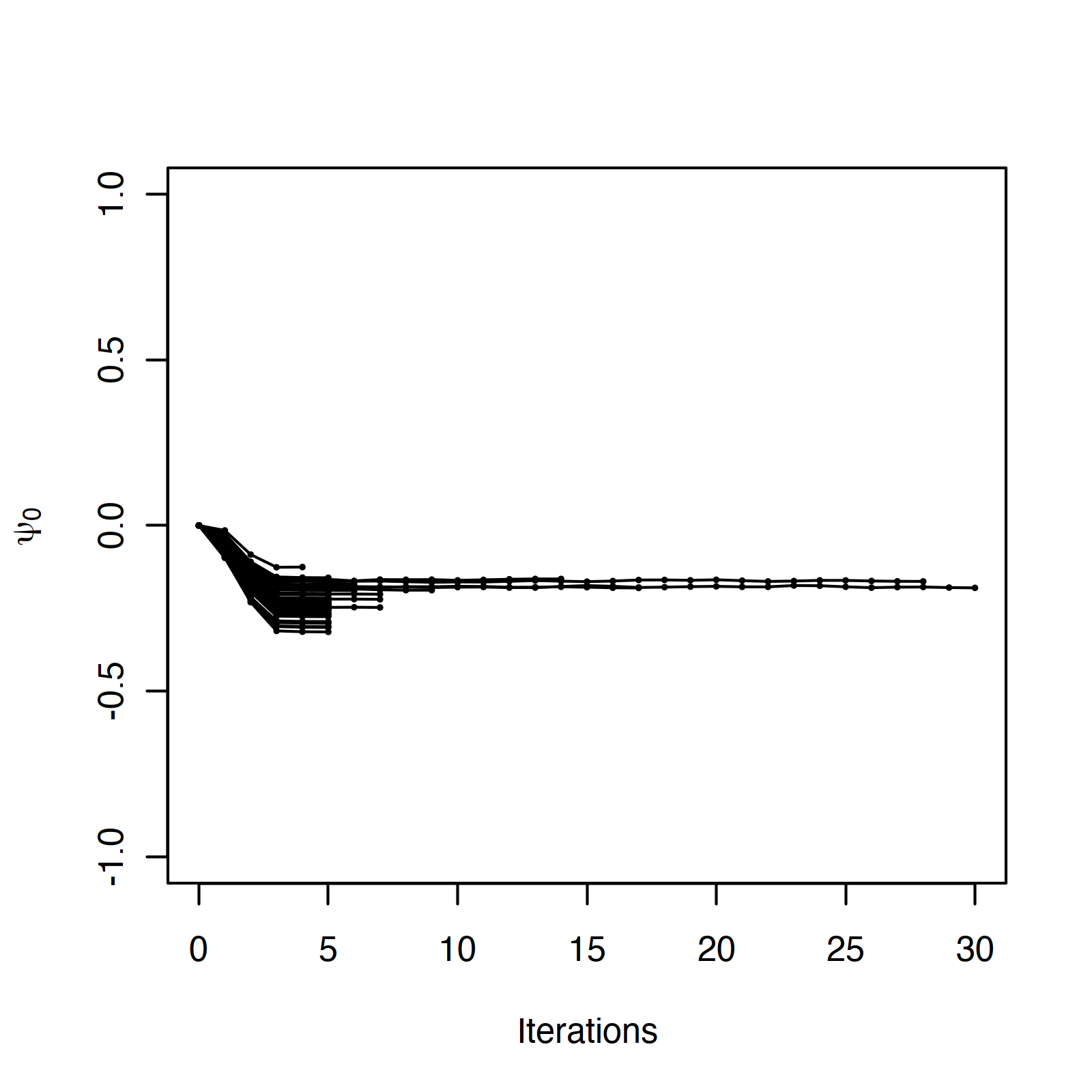
((e)) Penalized Q-shared: $\psi_{0}$

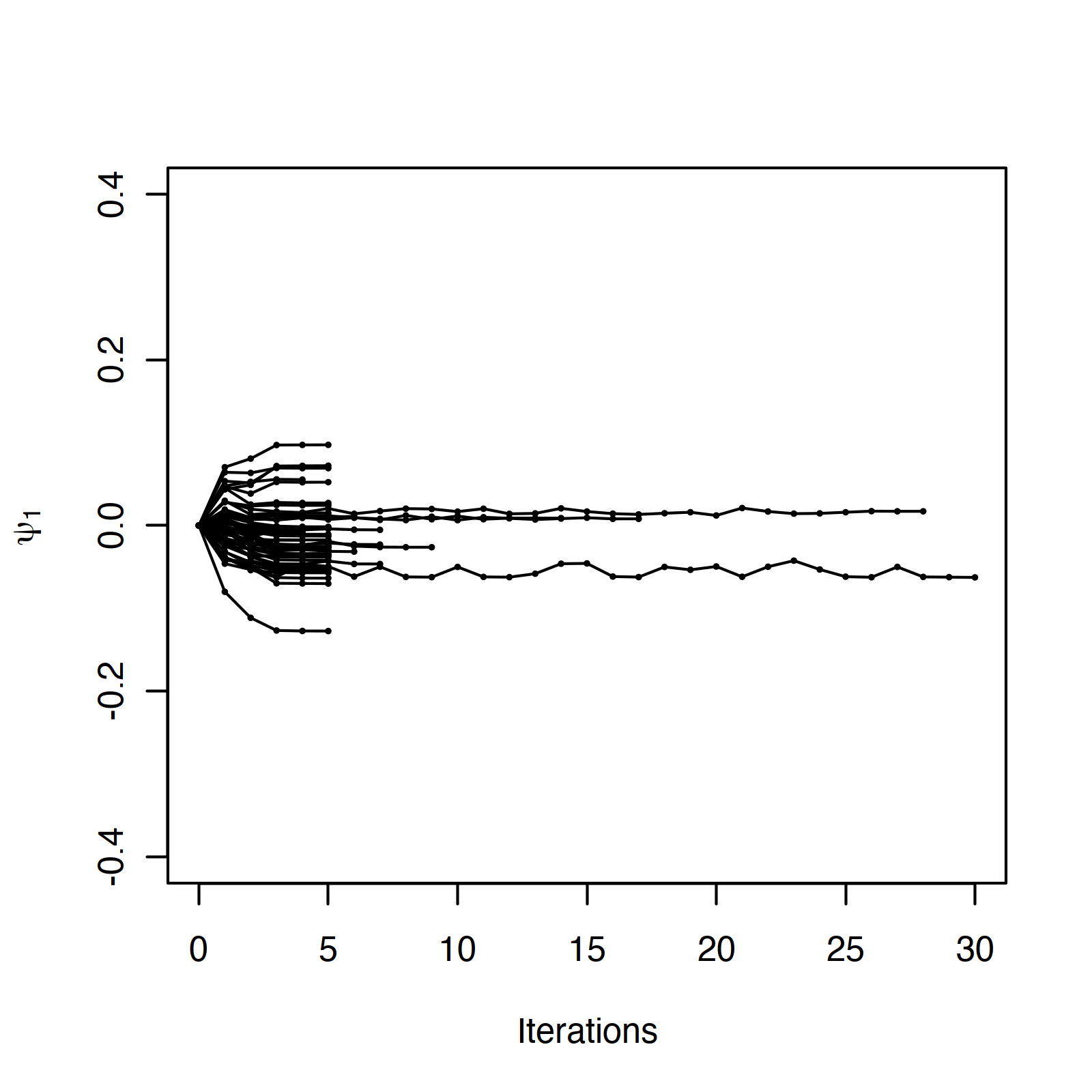
((f)) Penalized Q-shared: $\psi_{1}$

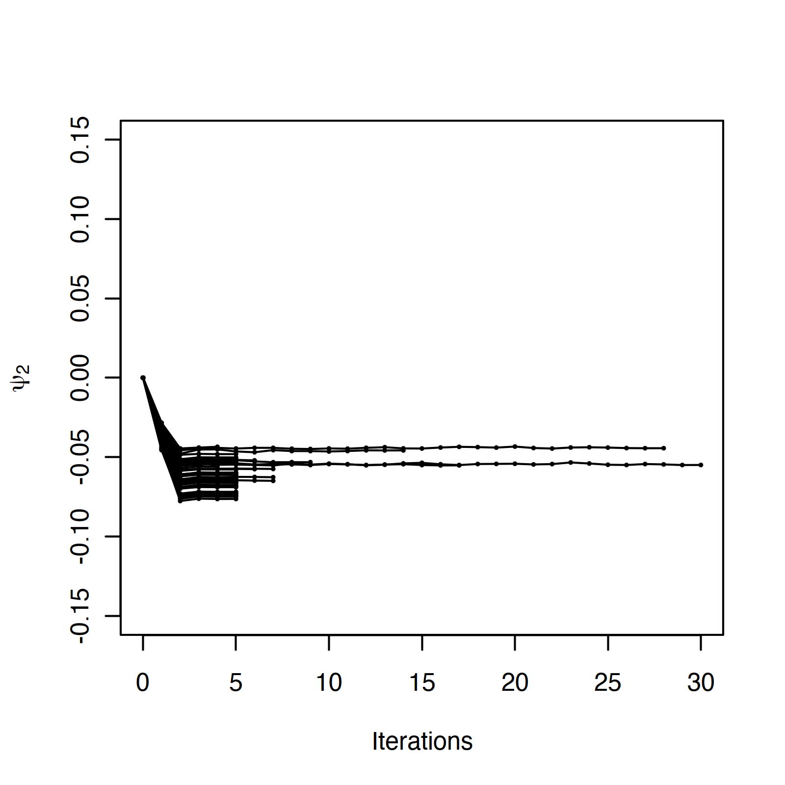
((g)) Penalized Q-shared: $\psi_{2}$

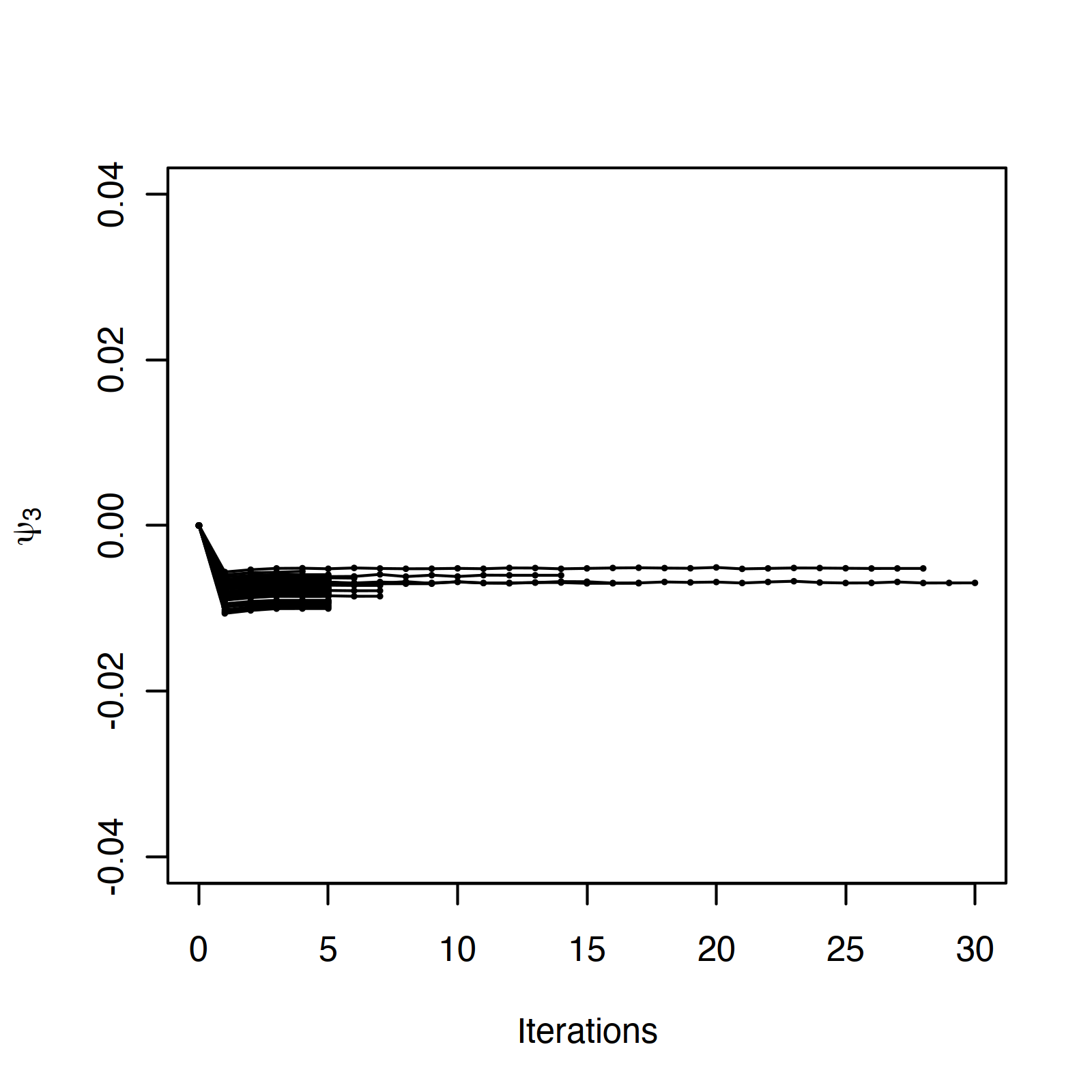
((h)) Penalized Q-shared: $\psi_{3}$

Figure 1: Showing the convergence pattern of Q-shared (top row) and penalized Q-shared (bottom row) based on 50 $m$-out-of-$n$ bootstrap samples. The initial values for all the cases have been set to zero.

Table 5: Estimates of the shared parameters along with their $m$-out-of-$n$ bootstrap variances and confidence intervals generated by the penalized Q-shared algorithm using the same data as in example 1.

		Using $m$-out-of-$n$ bootstrap
Shared Parameter	Estimate	Variance	CI
$\psi_{0}$	-0.1031	1.4471e-02	(-0.3357, 0.1298)
$\psi_{1}$	0.1890	1.3396e-02	(0.0322, 0.4395)
$\psi_{2}$	0.0096	1.2605e-04	(-0.0047, 0.0322)
$\psi_{3}$	-0.0004	1.4735e-06	(-0.0030, 0.0011)

Table 6: Estimates of the shared parameters along with their $m$-out-of-$n$ bootstrap variances and confidence intervals generated by the penalized Q-shared algorithm using the same data as in example 2.

		Using $m$-out-of-$n$ bootstrap
Shared Parameter	Estimate	Variance	CI
$\psi_{0}$	-0.2322	2.1751e-03	(-0.3170, -0.1560)
$\psi_{1}$	-0.0006	2.5419e-05	(-0.0093, 0.0079)
$\psi_{2}$	-0.0618	8.6451e-05	(-0.0777, -0.0444)
$\psi_{3}$	-0.0078	1.5672e-06	(-0.0097, -0.0055)

In a shared parameter DTR problem, ³ showed that the Q-shared algorithm works better than Q-unshared using simulation. In Table LABEL:Tab:_allocation-match, our objective is to illustrate that the penalized Q-shared algorithm performs better than the original Q-shared algorithm. We use the same set of examples and the same metrics for comparison, as in ³ to show the differences between two methods. As mentioned in section 4, the penalized Q-shared algorithm requires initial values of the parameters to start the algorithm. In Table LABEL:Tab:_allocation-match, we have considered five different choices of initial values of parameters. First, we have used Q-unshared to estimate $\theta_{j}^{T}=(\beta_{j}^{T},{\psi_{j}^{T}})$ as $\hat{\theta}_{j}^{(0)T}=(\hat{\beta}_{j}^{(0)T},{\hat{\psi}_{j}^{(0)T}}),j=1,\cdots,J$. Five different choices of the initial values of each of the shared parameter are: Simple Average (SA): $(1/J)\sum_{j=1}^{J}\hat{\psi}_{j}^{(0)}$; Inverse Variance Weighted Average (IVWA): $(\sum_{j=1}^{J}\frac{\hat{\psi}_{j}^{(0)}}{\hat{\sigma}_{j}^{2}})/(\sum_{j=1}^{J}\frac{1}{\hat{\sigma}_{j}^{2}})$, where the estimated large sample variance of $\hat{\psi}_{j}^{(0)}$ is $\hat{\sigma}_{j}^{2}$; MAX: $\max\{\hat{\psi}_{1}^{(0)},\cdots,\hat{\psi}_{J}^{(0)}\}$; MIN: $\min\{\hat{\psi}_{1}^{(0)},\cdots,\hat{\psi}_{J}^{(0)}\}$; ZERO: all the initial values of the parameters are taken as zero. Note that the initial values of the intercept parameter $\psi_{0}$ are calculated in similar ways for all the five different choices.

We consider two metrics: the weighted average of the stage-specific allocation matching ($M$) and overall allocation matching ($\tilde{M}$) over all the stages of the study. By matching, we mean the matching of treatment allocation between the method under consideration and an “oracle” method. The oracle method assumes that the Q-functions are correctly specified and the true values of the model parameters are known. Thus, the oracle DTR $d^{\psi_{oracle}}$ can allocate the best treatments over all the stages. To balance the different number of subjects across the different stages, the weighted average of the stage-specific allocation matching is defined as, $M=\frac{\sum_{j=1}^{J}n_{j}M_{j}}{\sum_{j=1}^{J}n_{j}}$, where $n_{j}$ denotes the number of patients at the $j^{th}$ stage, $M_{j}=P[d_{j}^{\hat{\psi}}(H_{j})=d_{j}^{\psi_{oracle}}(H_{j})]$ is the probability of allocation matching with the oracle at stage $j$ and $d_{j}^{\hat{\psi}}$ is the estimated DTR from the method under consideration. Similarly, the overall allocation matching is defined as, $\tilde{M}=P[d^{\hat{\psi}}=d^{\psi_{oracle}}]$ which denotes the probability of allocation matching over all the stages of the study for a subject.

Table 7: Comparison of Q-shared and penalized Q-shared algorithms with respect to bias of $\psi_{0}$ and allocation matching with the oracle (%) for sample size 300. The numbers for Q-shared have been recalculated and are same as in ³.

			Q-Shared			Penalized Q-Shared
7-9				Allocation Matching			Allocation Matching
Ex	$(\psi_{0},p_{3},p_{2})$	Method	Bias ($\psi_{0}$)	$\mathbf{M(\%)}$	$\mathbf{\tilde{M}(\%)}$	Bias ($\psi_{0}$)	$\mathbf{M(\%)}$	$\mathbf{\tilde{M}(\%)}$
1	(0.01,0,0)	Q-Shared.SA	0.0158	58.78	43.47	0.0269	62.73	49.00
		Q-Shared.IVWA	0.0154	59.08	43.74	0.0265	62.60	49.22
		Q-Shared.MAX	0.0156	59.23	43.90	0.0267	62.66	49.24
		Q-Shared.MIN	0.0154	59.14	43.80	0.0265	62.63	49.14
		Q-Shared.ZERO	0.0154	59.13	43.80	0.0266	62.71	49.28
2	(-0.05,0.5,0.5)	Q-Shared.SA	-0.0062	75.64	67.21	0.0016	75.22	66.76
		Q-Shared.IVWA	-0.0063	75.57	67.11	0.0014	75.89	67.85
		Q-Shared.MAX	-0.0061	75.52	67.15	0.0015	75.70	67.68
		Q-Shared.MIN	-0.0063	75.64	67.20	0.0013	75.87	67.84
		Q-Shared.ZERO	-0.0063	75.60	67.17	0.0014	75.73	67.67
3	(0.05,0.5,0)	Q-Shared.SA	-0.0134	67.42	51.45	-0.0139	70.26	55.45
		Q-Shared.IVWA	-0.0132	67.86	51.91	-0.0139	70.58	55.49
		Q-Shared.MAX	-0.0129	67.96	52.07	-0.0138	70.65	55.52
		Q-Shared.MIN	-0.0132	67.82	51.88	-0.0139	70.24	55.08
		Q-Shared.ZERO	-0.0132	67.83	51.94	-0.0138	70.61	55.51
4	(0.05,0,0)	Q-Shared.SA	-0.0119	69.53	54.13	-0.0175	69.02	53.62
		Q-Shared.IVWA	-0.0119	69.25	54.17	-0.0172	68.37	52.89
		Q-Shared.MAX	-0.0117	69.30	54.27	-0.0171	68.36	52.85
		Q-Shared.MIN	-0.0120	69.23	54.21	-0.0173	68.34	52.86
		Q-Shared.ZERO	-0.0119	69.17	54.21	-0.0172	68.24	52.63
5	(0.1,0.25,0)	Q-Shared.SA	0.0196	93.06	88.56	0.0069	94.67	91.01
		Q-Shared.IVWA	0.0199	93.29	88.96	0.0069	94.28	90.50
		Q-Shared.MAX	0.0201	93.38	89.08	0.0070	94.27	90.51
		Q-Shared.MIN	0.0199	93.27	88.97	0.0069	94.30	90.50
		Q-Shared.ZERO	0.0199	93.29	88.95	0.0069	94.28	90.48
6	(0.1,0.25,0.25)	Q-Shared.SA	0.0046	87.12	80.52	-0.0050	88.04	81.94
		Q-Shared.IVWA	0.0063	90.32	85.12	-0.0037	91.27	86.44
		Q-Shared.MAX	0.0064	90.46	85.30	-0.0036	91.29	86.45
		Q-Shared.MIN	0.0063	90.43	85.25	-0.0036	91.17	86.25
		Q-Shared.ZERO	0.0063	90.46	85.25	-0.0036	91.32	86.47
7	(-0.1,0,0)	Q-Shared.SA	-0.0055	89.26	79.65	0.0032	89.93	80.99
		Q-Shared.IVWA	-0.0053	88.55	78.75	0.0029	90.07	81.23
		Q-Shared.MAX	-0.0052	88.60	78.80	0.0030	90.04	81.20
		Q-Shared.MIN	-0.0053	88.62	78.77	0.0029	90.06	81.23
		Q-Shared.ZERO	-0.0052	88.65	78.81	0.0030	90.05	81.16

In this simulation study, we consider a three-stage ($J=3$) SMART design with 300 patients. At the end of each stage, those who are not doing well (called nonresponders) proceed to the next stage ($j$ to $j+1$), others who are doing well (called responders) proceed to a followup phase and exit the main study. Define $R_{1}$ and $R_{2}$ as the response indicators which takes 0 for nonresponder and 1 for responder at the end of first and second stages, respectively. Here, we generate $R_{1}$ and $R_{2}$ using a Bernoulli distribution with success probability 0.38 and 0.18, respectively. These values are obtained from the sequenced treatment alternatives to relieve depression (STAR*D) trial; our simulation study follow the same structure of this trial ¹⁷.

The stage-specific outcomes are generated as ³,

$$Y_{1}=\gamma_{1}+\gamma_{2}O_{1}+\gamma_{3}A_{1}+\gamma_{4}O_{1}A_{1}+\epsilon_{1},$$

$$Y_{2}=Y_{1}+\frac{3}{2}[\gamma_{5}O_{2}+\gamma_{6}A_{2}+\gamma_{7}O_{2}A_{2}+\gamma_{8}A_{1}A_{2}]+\epsilon_{2},$$

$$Y_{3}=Y_{2}+3[\gamma_{9}O_{3}+\gamma_{10}A_{3}+\gamma_{11}O_{3}A_{3}+\gamma_{12}A_{2}A_{3}+\gamma_{13}A_{1}A_{2}A_{3}]+\epsilon_{3},$$

where for $j=1,2,3$, the error terms $\epsilon_{i}\sim N(0,1)$, $A_{j}$ takes values 1 or -1 with equal probability (0.5); the covariate $O_{1}$ also takes values 1 or -1 with equal probability, $P(O_{2}=1|O_{1},A_{1})=1-P(O_{2}=-1|O_{1},A_{1})=\exp(\delta_{21}O_{1}+\delta_{22}A_{1})/(1+\exp(\delta_{21}O_{1}+\delta_{22}A_{1}))$ and $P(O_{3}=1|O_{1},A_{1},O_{2},A_{2})=1-P(O_{3}=-1|O_{1},A_{1},O_{2},A_{2})=\exp(\delta_{31}O_{2}+\delta_{32}A_{2}+\delta_{33}A_{1}A_{2})/(1+\exp(\delta_{31}O_{2}+\delta_{32}A_{2}+\delta_{33}A_{1}A_{2}))$. Note that, the primary outcome is defined as $Y_{Primary}=R_{1}Y_{1}+(1-R_{1})R_{2}((Y_{1}+Y_{2})/2)+(1-R_{1})(1-R_{2})((Y_{1}+Y_{2}+Y_{3})/3)$. Therefore, above expressions for $Y_{1},Y_{2}$ and $Y_{3}$ ensure that the final outcome for those who remain till the end ($R_{1}=R_{2}=0$) of third stage is $Y=\gamma_{1}+\gamma_{2}O_{1}+\gamma_{3}A_{1}+\gamma_{4}O_{1}A_{1}+\gamma_{5}O_{2}+\gamma_{6}A_{2}+\gamma_{7}O_{2}A_{2}+\gamma_{8}A_{1}A_{2}+\gamma_{9}O_{3}+\gamma_{10}A_{3}+\gamma_{11}O_{3}A_{3}+\gamma_{12}A_{2}A_{3}+\gamma_{13}A_{1}A_{2}A_{3}+\epsilon$, where $\epsilon=(\epsilon_{1}+\epsilon_{2}+\epsilon_{3})/3$. Given the $\gamma$-parameters, the above generative models generate a 3-stage SMART data for the simulation study. From this data, we develop DTRs using the following Q-functions:

$$Q_{3} = \beta_{30}+\beta_{31}O_{1}+\beta_{32}A_{1}+\beta_{33}O_{1}A_{1}+\beta_{34}O_{2}+\beta_{35}A_{2}+\beta_{36}O_{2}A_{2}+\beta_{37}A_{1}A_{2}+\beta_{38}O_{3}+(\psi_{0}+\psi_{1}O_{3}+\psi_{2}A_{2}+\psi_{3}A_{1}A_{2})A_{3},$$

$$Q_{2} = \beta_{20}+\beta_{21}O_{1}+\beta_{22}A_{1}+\beta_{23}O_{1}A_{1}+\beta_{24}O_{2}+(\psi_{0}+\psi_{1}O_{2}+\psi_{2}A_{1})A_{2},$$

$$Q_{1} = \beta_{10}+\beta_{11}O_{1}+(\psi_{0}+\psi_{1}O_{1})A_{1}.$$

Note that $\psi_{0}$ and $\psi_{1}$ are the shared parameters across all the three stages whereas $\psi_{2}$ is shared only between stages 2 and 3. To calculate the bias of different parameters, the relationship between $\gamma$s and $\beta$s are given in ³. In Table LABEL:Tab:_allocation-match, the extent of nonregularity (due to non-smooth maximization) is given by $p_{3}=P(\psi^{T}H_{31}=0)$ and $p_{2}=P(\psi^{T}H_{21}=0)$ corresponding to stages 3 and 2 which can cause bias in parameter estimation in stages 2 and 1, respectively.

We can observe from Table LABEL:Tab:_allocation-match that penalized Q-shared algorithm performs better in all the examples except in example 4 and for the simple average (SA) version of the algorithms in example 2 with respect to both metrics $M$ and $\tilde{M}$. In some cases, the gain in allocation matching is high. For example, in example 3, there is around 3 to 4% increase in allocation matching with respect to both the metrics. Overall, we notice that the allocation matching does not depend on the choice of initial values for both the Q-shared and the penalized Q-shared algorithms. Interestingly, both the algorithms perform well based on initial values of all the parameter set to zero. Based on these observations, we can say that the developed penalized Q-shared algorithm is quite robust to the choice of initial values of the parameters. We have reported the bias of only $\psi_{0}$ as it represents the ‘main effect’ of treatment $A_{j}$ at the $j^{th}$ stage. In examples 2, 6 and 7, the estimated biases of $\psi_{0}$ are of opposite signs corresponding to each set of initial values. Also, the ‘sign’ of the estimated biases from the penalized Q-shared method are in the opposite direction of the true ‘sign’ of $\psi_{0}$ parameter values in those examples. However, in all those cases, the penalized Q-shared performs well compared to Q-shared. Note that, the sign of the contrast function ($\psi^{T}H_{j1},j=1,2,3$) decides the treatment allocation. Therefore, sometimes a little bias may help to decide the sign in a way to do better treatment allocation. This phenomenon is also observed in classification. For example, a support vector machine that can constitute “high margin classifiers" gives better allocation performance because of moving the margin a little far from the decision boundary. It also supports the idea of putting more emphasis on allocation matching performance than the bias of the estimated parameters.

6 Application to Real data

We have applied the penalized Q-shared algorithm to the three-stage STAR*D data to estimate the optimal shared-parameter DTR in the context of a major depressive disorder. A detailed description of the STAR*D trial that consists of 4041 patients is available from ¹⁷. For simplicity, here we consider binary treatment ($A_{j}$) at each stage ($j=1,2,3$) as mono therapy (coded as 1) and combination therapy (coded as -1), and other setup is also the same as ³. The primary outcome ($Y_{primary}$) is the same as defined in section 3 as a function of stage specific outcomes $Y_{1},Y_{2}$ and $Y_{3}$ and response indicators ($R_{1},R_{2}$). Here, $Y_{j},j=1,2,3$ denotes -QIDS (rated by clinician). The negative sign before QIDS makes the outcome such that the higher is the better, since a lower QIDS score indicates an improvement of a patient outcome. Therefore, $Y_{primary}$ denotes an average -QIDS score of an individual during their stay in the trial. We consider four tailoring variables (covariates), initial QIDS score at the start of a stage ($start.QIDS_{j}$), observed slope of the QIDS score from the previous stage ($slope.QIDS_{j}$), presence or absence of side effect from the earlier stage ($side.effect_{j}$) and earlier stage binary treatment ($A_{j-1}\in\{-1,1\}$, j=2,3). We consider the following Q-functions ³:

$$Q_{3}(H_{3},A_{3}) = \beta_{03}+\beta_{13}\times start.QIDS_{3}+\beta_{23}\times slope.QIDS_{3}+\beta_{33}\times side.effect_{3}+\beta_{43}\times A_{2}$$

$$+(\psi_{0}+\psi_{1}\times start.QIDS_{3}+\psi_{2}\times slope.QIDS_{3}+\psi_{3}\times side.effect_{3}+\psi_{4}\times A_{2})\times A_{3}$$

$$Q_{2}(H_{2},A_{2}) = \beta_{02}+\beta_{12}\times start.QIDS_{2}+\beta_{22}\times slope.QIDS_{2}+\beta_{32}\times side.effect_{2}+\beta_{42}\times A_{1}$$

$$+(\psi_{0}+\psi_{1}\times start.QIDS_{2}+\psi_{2}\times slope.QIDS_{2}+\psi_{3}\times side.effect_{2}+\psi_{4}\times A_{1})\times A_{2}$$

$$Q_{2}(H_{1},A_{1}) = \beta_{01}+\beta_{11}\times start.QIDS_{1}+\beta_{21}\times slope.QIDS_{1}$$

$$+(\psi_{0}+\psi_{1}\times start.QIDS_{1}+\psi_{2}\times slope.QIDS_{1})\times A_{1}$$

Note that, the side effect from the previous stage for stage 1 is not considered as everyone obtained the same treatment (citalopram) before entering stage 1. Table 8 shows the estimated shared parameters using penalized Q-shared algorithm along with $m$-out-of-$n$ bootstrap variances and 95% confidence intervals. Observe that the only significant shared parameter is $\psi_{2}$. This finding from STAR*D data is consistent with that using Q-shared algorithm mentioned in ³. Using the estimated values of shared parameters, the stage-specific optimal DTR are

$$d_{3}(H_{3}) = sign(-0.0298+0.0052\times start.QIDS_{3}-0.0700\times slope.QIDS_{3}+0.0086\times side.effect_{3}+0.0060\times A_{2}),$$

$$d_{2}(H_{2}) = sign(-0.0298+0.0052\times start.QIDS_{2}-0.0700\times slope.QIDS_{2}+0.0086\times side.effect_{2}+0.0060\times A_{1}),$$

$$d_{1}(H_{1}) = sign(-0.0298+0.0052\times start.QIDS_{1}-0.0700\times slope.QIDS_{1}).$$

In practice, we will know the stage-specific values of $start.QIDS$, $slope.QIDS$, $side.effect$ and the previous stage treatment for a patient. Therefore using the above DTRs, one can decide whether to give mono therapy (1) or combination therapy (-1) to that patient in a particular stage.

Table 8: Estimates of the shared parameters along with their $m$-out-of-$n$ bootstrap variances and confidence intervals generated by penalized Q-shared algorithm using the STAR*D data. Here the binary treatment is coded as {-1, 1}.

		Using $m$-out-of-$n$ bootstrap
Shared Parameter	Estimate	Variance	CI
$\psi_{0}$	-0.0298	0.0010	(-0.0901, 0.0290)
$\psi_{1}$	0.0052	8.6309	(-0.0141, 0.0220)
$\psi_{2}$	-0.0700	0.0014	(-0.1378, -0.0001)
$\psi_{3}$	0.0086	0.0007	(-0.0436, 0.0584)
$\psi_{4}$	0.0060	0.0017	(-0.0786, 0.0876)

7 Conclusion

In this work, we have shown that the penalized Q-shared algorithm is a better algorithm than the original Q-shared algorithm. The Q-shared algorithm needs to estimate fewer parameters than a Q-learning algorithm to develop DTRs for the same data with shared decision rules. We have demonstrated that penalized Q-shared outperforms Q-shared even in settings where there are no convergence issues. Thus, researchers may use the penalized Q-shared method over Q-shared in all the cases. Our work demonstrates empirical improvements through regularization. Critical work remains to establish theoretical guarantees of convergence.

8 Acknowledgements

Trikay Nalamada and Shruti Agarwal acknowledge support from Samsung Fellowship. Bibhas Chakraborty acknowledges support from the Duke-NUS Medical School, Singapore. Palash Ghosh acknowledges support from the Start-up Grant (PG001), Indian Institute of Technology Guwahati. This manuscript reflects the views of the authors only.

9 DATA AVAILABILITY STATEMENT

We used the limited access datasets distributed from the National Institute of Mental Health (NIMH), USA.

References

- Almirall \BOthers. \APACyear2016 \APACinsertmetastaralmirall2016Autism{APACrefauthors}Almirall, D., DiStefano, C., Chang, Y\BHBIC., Shire, S., Kaiser, A., Lu, X.\BDBLKasari, C. \APACrefYearMonthDay2016. \BBOQ\APACrefatitleLongitudinal effects of adaptive interventions with a speech-generating device in minimally verbal children with ASD Longitudinal effects of adaptive interventions with a speech-generating device in minimally verbal children with asd.\BBCQ \APACjournalVolNumPagesJournal of Clinical Child & Adolescent Psychology454442–456. \PrintBackRefs\CurrentBib
- Almirall \BOthers. \APACyear2014 \APACinsertmetastarAlmirall2014{APACrefauthors}Almirall, D., Nahum-Shani, I., Sherwood, N\BPBIE.\BCBL \BBA Murphy, S\BPBIA. \APACrefYearMonthDay2014Sep01. \BBOQ\APACrefatitleIntroduction to SMART designs for the development of adaptive interventions: with application to weight loss research Introduction to SMART designs for the development of adaptive interventions: with application to weight loss research.\BBCQ \APACjournalVolNumPagesTranslational Behavioral Medicine43260–274. {APACrefURL} https://doi.org/10.1007/s13142-014-0265-0 {APACrefDOI} 10.1007/s13142-014-0265-0 \PrintBackRefs\CurrentBib
- Chakraborty \BOthers. \APACyear2016 \APACinsertmetastarChak_2016{APACrefauthors}Chakraborty, B., Ghosh, P., Moodie, E\BPBIE\BPBIM.\BCBL \BBA Rush, A\BPBIJ. \APACrefYearMonthDay2016. \BBOQ\APACrefatitleEstimating optimal shared-parameter dynamic regimens with application to a multistage depression clinical trial Estimating optimal shared-parameter dynamic regimens with application to a multistage depression clinical trial.\BBCQ \APACjournalVolNumPagesBiometrics723865-876. {APACrefURL} http://dx.doi.org/10.1111/biom.12493 {APACrefDOI} 10.1111/biom.12493 \PrintBackRefs\CurrentBib
- Chakraborty \BOthers. \APACyear2013 \APACinsertmetastarchak_laber12{APACrefauthors}Chakraborty, B., Laber, E.\BCBL \BBA Zhao, Y. \APACrefYearMonthDay2013. \BBOQ\APACrefatitleInference for optimal dynamic treatment regimes using an adaptive -out-of- bootstrap scheme Inference for optimal dynamic treatment regimes using an adaptive -out-of- bootstrap scheme.\BBCQ \APACjournalVolNumPagesBiometrics69714 - 723. \PrintBackRefs\CurrentBib
- Chakraborty \BBA Moodie \APACyear2013 \APACinsertmetastarChak_book{APACrefauthors}Chakraborty, B.\BCBT \BBA Moodie, E. \APACrefYear2013. \APACrefbtitleStatistical Methods for Dynamic Treatment Regimes: Reinforcement Learning, Causal Inference, and Personalized Medicine Statistical methods for dynamic treatment regimes: Reinforcement learning, causal inference, and personalized medicine. \APACaddressPublisherNew YorkSpringer. \PrintBackRefs\CurrentBib
- Committee \BOthers. \APACyear2009 \APACinsertmetastarinternational2009international{APACrefauthors}Committee, I\BPBIE.\BCBT \BOthersPeriod. \APACrefYearMonthDay2009. \BBOQ\APACrefatitleInternational Expert Committee report on the role of the A1C assay in the diagnosis of diabetes International expert committee report on the role of the a1c assay in the diagnosis of diabetes.\BBCQ \APACjournalVolNumPagesDiabetes Care3271327–1334. \PrintBackRefs\CurrentBib
- Eden \APACyear2017 \APACinsertmetastareden2017field{APACrefauthors}Eden, D. \APACrefYearMonthDay2017. \BBOQ\APACrefatitleField experiments in organizations Field experiments in organizations.\BBCQ \APACjournalVolNumPagesAnnual Review of Organizational Psychology and Organizational Behavior491–122. \PrintBackRefs\CurrentBib
- Friedman \BOthers. \APACyear2010 \APACinsertmetastarfriedman2010regularization{APACrefauthors}Friedman, J., Hastie, T.\BCBL \BBA Tibshirani, R. \APACrefYearMonthDay2010. \BBOQ\APACrefatitleRegularization paths for generalized linear models via coordinate descent Regularization paths for generalized linear models via coordinate descent.\BBCQ \APACjournalVolNumPagesJournal of Statistical Software3311. \PrintBackRefs\CurrentBib
- Ghosh \BOthers. \APACyear2020 \APACinsertmetastarGhosh2020noninfi{APACrefauthors}Ghosh, P., Nahum-Shani, I., Spring, B.\BCBL \BBA Chakraborty, B. \APACrefYearMonthDay2020. \BBOQ\APACrefatitleNoninferiority and equivalence tests in sequential, multiple assignment, randomized trials (SMARTs). Noninferiority and equivalence tests in sequential, multiple assignment, randomized trials (SMARTs).\BBCQ \APACjournalVolNumPagesPsychological Methods252182. \PrintBackRefs\CurrentBib
- Hastie \BOthers. \APACyear2009 \APACinsertmetastarhastie2009elements{APACrefauthors}Hastie, T., Tibshirani, R.\BCBL \BBA Friedman, J. \APACrefYear2009. \APACrefbtitleThe elements of statistical learning: data mining, inference, and prediction The elements of statistical learning: data mining, inference, and prediction. \APACaddressPublisherSpringer Science & Business Media. \PrintBackRefs\CurrentBib
- Kidwell \APACyear2014 \APACinsertmetastarkidwell2014smart{APACrefauthors}Kidwell, K\BPBIM. \APACrefYearMonthDay2014. \BBOQ\APACrefatitleSMART designs in cancer research: past, present, and future SMART designs in cancer research: past, present, and future.\BBCQ \APACjournalVolNumPagesClinical trials114445–456. \PrintBackRefs\CurrentBib
- Lizotte \APACyear2011 \APACinsertmetastarlizotte2011convergent{APACrefauthors}Lizotte, D. \APACrefYearMonthDay2011. \BBOQ\APACrefatitleConvergent fitted value iteration with linear function approximation Convergent fitted value iteration with linear function approximation.\BBCQ \APACjournalVolNumPagesAdvances in Neural Information Processing Systems242537–2545. \PrintBackRefs\CurrentBib
- Murphy \APACyear2003 \APACinsertmetastarmurphy03{APACrefauthors}Murphy, S. \APACrefYearMonthDay2003. \BBOQ\APACrefatitleOptimal dynamic treatment regimes (with discussions) Optimal dynamic treatment regimes (with discussions).\BBCQ \APACjournalVolNumPagesJournal of the Royal Statistical Society, Series B65331 - 366. \PrintBackRefs\CurrentBib
- Murphy \APACyear2005 \APACinsertmetastarmurphy05b{APACrefauthors}Murphy, S. \APACrefYearMonthDay2005. \BBOQ\APACrefatitleA generalization error for Q-learning A generalization error for Q-learning.\BBCQ \APACjournalVolNumPagesJournal of Machine Learning Research61073 - 1097. \PrintBackRefs\CurrentBib
- Nahum-Shani \BOthers. \APACyear2015 \APACinsertmetastarnahum2015Health_psycho{APACrefauthors}Nahum-Shani, I., Hekler, E\BPBIB.\BCBL \BBA Spruijt-Metz, D. \APACrefYearMonthDay2015. \BBOQ\APACrefatitleBuilding health behavior models to guide the development of just-in-time adaptive interventions: A pragmatic framework. Building health behavior models to guide the development of just-in-time adaptive interventions: A pragmatic framework.\BBCQ \APACjournalVolNumPagesHealth Psychology34S1209. \PrintBackRefs\CurrentBib
- Robins \APACyear2004 \APACinsertmetastarrobins04{APACrefauthors}Robins, J. \APACrefYearMonthDay2004. \BBOQ\APACrefatitleOptimal structural nested models for optimal sequential decisions Optimal structural nested models for optimal sequential decisions.\BBCQ \BIn D. Lin \BBA P. Heagerty (\BEDS), \APACrefbtitleProceedings of the Second Seattle Symposium on Biostatistics Proceedings of the second seattle symposium on biostatistics (\BPG 189 - 326). \APACaddressPublisherNew YorkSpringer. \PrintBackRefs\CurrentBib
- Rush \BOthers. \APACyear2004 \APACinsertmetastarrush04{APACrefauthors}Rush, A\BPBIJ., Fava, M., Wisniewski, S., Lavori, P., Trivedi, M., Sackeim, H.\BDBLNiederehe, G. \APACrefYearMonthDay2004. \BBOQ\APACrefatitleSequenced treatment alternatives to relieve depression (STAR*D): Rationale and design Sequenced treatment alternatives to relieve depression (STAR*D): Rationale and design.\BBCQ \APACjournalVolNumPagesControlled Clinical Trials25119 - 142. \PrintBackRefs\CurrentBib
- Rush \BOthers. \APACyear2003 \APACinsertmetastarrush2003QUID{APACrefauthors}Rush, A\BPBIJ., Trivedi, M\BPBIH., Ibrahim, H\BPBIM., Carmody, T\BPBIJ., Arnow, B., Klein, D\BPBIN.\BDBLothers \APACrefYearMonthDay2003. \BBOQ\APACrefatitleThe 16-Item Quick Inventory of Depressive Symptomatology (QIDS), clinician rating (QIDS-C), and self-report (QIDS-SR): a psychometric evaluation in patients with chronic major depression The 16-item quick inventory of depressive symptomatology (qids), clinician rating (qids-c), and self-report (qids-sr): a psychometric evaluation in patients with chronic major depression.\BBCQ \APACjournalVolNumPagesBiological Psychiatry545573–583. \PrintBackRefs\CurrentBib
- Song, Kosorok\BCBL \BOthers. \APACyear2015 \APACinsertmetastarsong2015sparse{APACrefauthors}Song, R., Kosorok, M., Zeng, D., Zhao, Y., Laber, E.\BCBL \BBA Yuan, M. \APACrefYearMonthDay2015. \BBOQ\APACrefatitleOn sparse representation for optimal individualized treatment selection with penalized outcome weighted learning On sparse representation for optimal individualized treatment selection with penalized outcome weighted learning.\BBCQ \APACjournalVolNumPagesSTAT4159–68. \PrintBackRefs\CurrentBib
- Song, Wang\BCBL \BOthers. \APACyear2015 \APACinsertmetastarRuiSong2015{APACrefauthors}Song, R., Wang, W., Zeng, D.\BCBL \BBA Kosorok, M\BPBIR. \APACrefYearMonthDay2015. \BBOQ\APACrefatitlePENALIZED Q-LEARNING FOR DYNAMIC TREATMENT REGIMENS Penalized Q-learning for dynamic treatment regimens.\BBCQ \APACjournalVolNumPagesStatistica Sinica253901–920. {APACrefURL} http://www.jstor.org/stable/24721213 \PrintBackRefs\CurrentBib
- Villain \BOthers. \APACyear2019 \APACinsertmetastarvillain2019adaptive{APACrefauthors}Villain, L., Commenges, D., Pasin, C., Prague, M.\BCBL \BBA Thiébaut, R. \APACrefYearMonthDay2019. \BBOQ\APACrefatitleAdaptive protocols based on predictions from a mechanistic model of the effect of IL7 on CD4 counts Adaptive protocols based on predictions from a mechanistic model of the effect of IL7 on CD4 counts.\BBCQ \APACjournalVolNumPagesStatistics in Medicine382221–235. \PrintBackRefs\CurrentBib
- Walkington \APACyear2013 \APACinsertmetastarWalkington2013Education{APACrefauthors}Walkington, C\BPBIA. \APACrefYearMonthDay2013. \BBOQ\APACrefatitleUsing adaptive learning technologies to personalize instruction to student interests: The impact of relevant contexts on performance and learning outcomes. Using adaptive learning technologies to personalize instruction to student interests: The impact of relevant contexts on performance and learning outcomes.\BBCQ \APACjournalVolNumPagesJournal of Educational Psychology1054932. \PrintBackRefs\CurrentBib
- Zhang \BOthers. \APACyear2012 \APACinsertmetastarZhang12a{APACrefauthors}Zhang, B., Tsiatis, A., Davidian, M., Zhang, M.\BCBL \BBA Laber, E. \APACrefYearMonthDay2012. \BBOQ\APACrefatitleEstimating optimal treatment regimes from a classification perspective Estimating optimal treatment regimes from a classification perspective.\BBCQ \APACjournalVolNumPagesSTAT1103-114. \PrintBackRefs\CurrentBib
- Zhao \BOthers. \APACyear2020 \APACinsertmetastarzhao2020Shared_Censored{APACrefauthors}Zhao, Y\BHBIQ., Zhu, R., Chen, G.\BCBL \BBA Zheng, Y. \APACrefYearMonthDay2020. \BBOQ\APACrefatitleConstructing dynamic treatment regimes with shared parameters for censored data Constructing dynamic treatment regimes with shared parameters for censored data.\BBCQ \APACjournalVolNumPagesStatistics in Medicine3991250–1263. \PrintBackRefs\CurrentBib