Turbulence-immune computational ghost imaging based on a multi-scale generative adversarial network

Abstract

There is a consensus that turbulence-free images cannot be obtained by conventional computational ghost imaging (CGI) because the CGI is only a classic simulation, which does not satisfy the conditions of turbulence-free imaging. In this article, we first report a turbulence-immune CGI method based on a multi-scale generative adversarial network (MsGAN). Here, the conventional CGI framework is not changed, but the conventional CGI coincidence measurement algorithm is optimized by an MsGAN. Thus, the satisfactory turbulence-free ghost image can be reconstructed by training the network, and the visual effect can be significantly improved.

Key words: computational ghost imaging; atmospheric turbulence; multi-scale generative adversarial network

PACS codes: 42.30.Va, 42.30.-d, 42.25.Kb

Ghost imaging (GI) can be traced to the pioneering work initiated by Shih et.al. [1], who exploited biphotons generated via spontaneous parametric down-conversion to realize the first entanglement-based ghost image, following the original proposals by Klyshko [2]. The framework of quantum entangled light source determines that the initial GI requires two light paths [1]. One of the beams is the reference beam, which never illuminates the object and is directly measured by a detector with spatial resolution. The other beam is the object beam, which, after illuminating the object, is measured by a bucket detector with no spatial resolution. By correlating the photocurrents from the two detectors, one retrieves the “ghost” image. In the debate of the physical essence of GI [3], pseudothermal ghost imaging [4,5] and pure thermal ghost imaging [6] have been successively confirmed, which is great progress for GI. However, the conventional GI is not suitable for practical applications because the structure of the two optical paths limits the flexibility of the optical system. Fortunately, Shapiro proposed a single optical path GI scheme: computational ghost imaging (CGI) [7,8]. Because it has only one optical path, the imaging frame is closer to classical optical imaging. Consequently, it has important potential applications in remote sensing [9-11], lidar [12-16] and night vision imaging [17,18].

Atmospheric turbulence is a serious problem for satellite remote sensing and aircraft-to-ground-based classical imaging. Surprisingly, Meyers et. al. found that a turbulence-free image could be obtained by conventional dual-path GI in 2011 [19-21]. This unique and practical property is an important milestone for optical imaging because any fluctuation index disturbance introduced in the optical path will not affect the image quality. Shih et. al. revealed that the turbulence-free effect was due to the two-photon interference [21,22]. Li et. al. summarized the necessary conditions for turbulence-free imaging [23]. However, CGI is a classical simulation of GI, so it does not satisfy the conditions of turbulence-free imaging [22]. At present, this conclusion is generally accepted. Even to this day, it is a challenge work to realize turbulence-free CGI. Fortunately, generative adversarial network provides a promising solution for this [24,25].

In this article, we demonstrate that turbulence-immune CGI can be realized by a multi-scale generative adversarial network (MsGAN). In this scheme, the basic framework of conventional CGI is not changed. Correspondingly, we optimize the coincidence measurement algorithm of CGI by an MsGAN. In atmospheric turbulence environment, the satisfactory ghost images can be reconstructed by training the network. In the following, we theoretically and experimentally illustrate this method.

We depict the scheme in Fig. 1. A quasi-monochromatic laser illuminates an object $T\left(\rho\right)$; then, the reflected light carrying the object’s information is received and modulated by a spatial light modulator (SLM). A photomultiplier tube (PMT) collects the light intensity $E_{di}\left(\rho,t\right)$. Correspondingly, the calculated light $E_{ci}\left(\rho^{{}^{\prime}},t\right)$ can be obtained by diffraction theory. By processing the two light signals with a conventional CGI algorithm, the object’s image can be reconstructed, i.e.,

$$G(\rho,\rho^{{}^{\prime}}) =\frac{1}{n}{\displaystyle\sum\limits_{i=1}^{n}}\left(\left\langle\left|E_{di}(\rho,t)\right|^{2}\left|E_{ci}(\rho,t)\right|^{2}\right\rangle\right.$$

$$-\left.\left\langle\left|E_{di}(\rho,t)\right|^{2}\right\rangle\left\langle\left|E_{ci}(\rho,t)\right|^{2}\right\rangle\right),$$ (1)

where $\left\langle\cdot\right\rangle$ is an ensemble average. The subscript $i=1,2,...n$ denotes the $i$th measurement, and $n$ is the total number of measurements.

The flow chart of the MsGAN is shown in Fig. 2. The scheme mainly consists of three parts: (i) a conventional CGI algorithm to obtain distorted images; (ii) a generator G of MsGAN to generate random data into sample images through continuous training; (iii) a discriminator D of MsGAN to distinguish generated samples from real images.

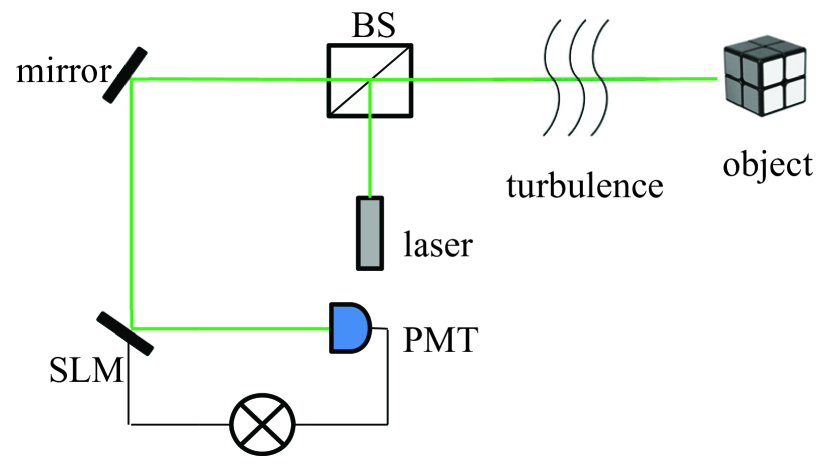
Figure 1: Setup of the computational ghost imaging. BS: beam splitter, SLM: spatial light modulator, PMT: photomultiplier tube.

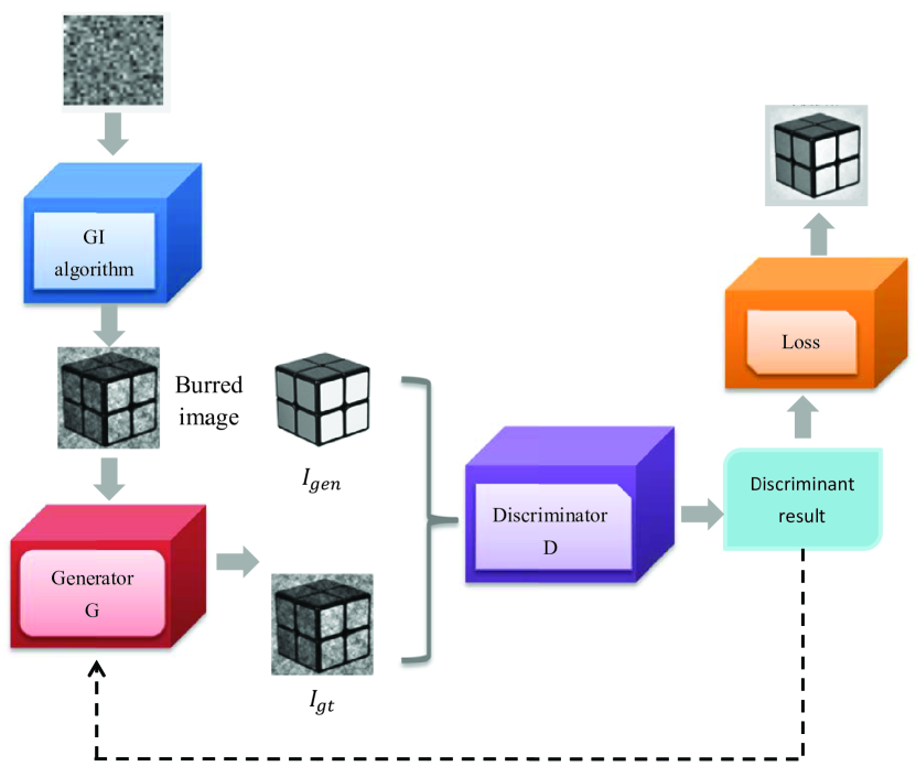
Figure 2: Network structure of the MsGAN.

The network structure of generator G is shown in Fig. 3. The basic framework is a symmetric U-Net architecture. On this basis, multi-scale attention feature extraction units and a multi-level feature dynamic fusion unit are added to the U-Net architecture. The multi-scale attention feature extraction units use convolution kernels of different sizes to extract multi-scale feature information in larger receptive fields. The multi-level feature fusion unit can dynamically fuse feature images with different proportions by adjusting the weight and excavating the semantic information of different levels. Since U-Net will lose detailed features of the images in the process of encoding and decoding, the visual detail features of the reconstructed image can be improved by adding skip connections as hierarchical semantic guidance. The network mainly consists of a full convolution part and an up-sampling part. The full convolution part of the U-Net consists of a pre-training convolution module and multi-scale attention feature extraction units. The pre-trained convolution module uses the convolution layer and max-pooling layer of the Inception-ResNet-v2 backbone network.

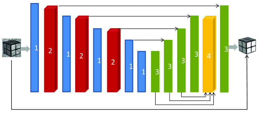
Figure 3: Network structure of the generator G. 1 represents the pre-trained convolution module; 2 represents a multi-scale attention feature extraction unit; 3 represents an up-sampling layer and 4 represents a multi-level feature dynamic fusion unit.

The multi-scale attention feature extraction units are composed of multi-branch convolution layers and an attention layer (Fig. 4). The multi-branch convolution layers are composed of different sizes of juxtaposed dilated convolutions, which correspond to different sizes of receptive fields, to extract various features. Three branches with receptive fields of $3\times 3$, $5\times 5$, and $7\times 7$ simultaneously extract features of the input images. After the information feature graphs of different scales are obtained, the cascaded feature graphs are readjusted to the input size through the convolution operation.

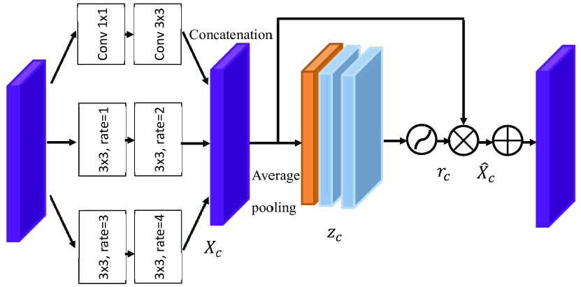
Figure 4: Structure of multi-scale attention feature extraction units.

In feature extraction, an attention mechanism is introduced to generate different attention for each channel feature to distinguish between low-frequency parts (smooth or flat areas) and high-frequency parts (such as lines, edges, and textures) of images to pay attention to and learn the key content of the image. First, the global context information of each channel is used to compress the spatial information of each channel by global average pooling. The expression is

$$z_{c}=G_{p}\left(X_{c}\right)=\frac{1}{H\times W}{\displaystyle\sum\limits_{i=1}^{H}}{\displaystyle\sum\limits_{j=1}^{W}}X_{c}\left(i,j\right)$$ (2)

where $X_{c}$ is the aggregation convolution feature graph with the size of $H\times W\times C$, and $Z_{c}$ is the compressed global pooling layer with the size of $1\times 1\times C$. ReLU and Sigmoid activation functions are used to implement the gating principle to learn the nonlinear synergistic effect and mutual exclusion relationship between channels, and the attention mechanism can be expressed as

$$r_{c} =\sigma\left\{Conv\left[\delta\left(Conv\left(z_{c}\right)\right)\right]\right\},$$ (3)

$$\overset{\char 94\relax}{X_{c}} =r_{c}\times X_{c},$$ (4)

where $\delta$ and $\sigma$ are the activation functions of ReLU and sigmoid, respectively, $r_{c}$ is the weight of excitation, $\overset{\char 94\relax}{X_{c}}$ is the feature graph after the adjustment of the attention mechanism. The global pooling layer $z_{c}$ goes through the down-sampling convolutional layer and ReLU activation function, and the channel number is recovered through the up-sampling convolutional layer. Finally, it is activated by the sigmoid function to obtain the channel excitation weight $r_{c}$. The value of the aggregation convolution layer $X_{c}$ channel is multiplied by different weights to obtain the output $\overset{\char 94\relax}{X_{c}}$ of the adaptive adjustment channel attention.

The up-sampling part of the U-Net architecture includes up-sampling layers and a multi-level feature dynamic fusion unit. In the up-sampling part of the generator network, the feature graphs at different levels contain different instance information. A multi-level feature fusion unit is proposed to enhance the information transfer among feature maps at different levels. In addition, we propose a dynamic fusion network structure to solve the problem of feature conflict at different levels. The method assigns different weights to the spatial position of the feature map to screen the valid features and filter out contradictory information through learning. First, the feature images of different scales are adjusted to the same size by up-sampling, and spatial weights are set for feature images of different levels during fusion to find the optimal fusion strategy. It can be specifically expressed as:

$$F^{\ast}=\omega_{1}\times F^{1\uparrow}+\omega_{2}\times F^{2\uparrow}+\omega_{3}\times F^{3\uparrow}+\omega_{4}\times F^{4\uparrow},$$ (5)

where $\omega_{i}$ is the weight corresponding to feature graphs of different levels, $F^{i\uparrow}$ is the standard feature graph of the $i$th feature graph adjusted to a uniform size after up-sampling, $F^{\ast}$ is the final feature graph output by dynamic fusion of all levels of features through adaptive weight allocation. In the end, generator G introduces a skip connection directly from the input to the output, which forces the model to focus on learning residuals.

We input the feature images generated by generator G and the real images into discriminator D for discrimination. Discriminator D adopts the PatchGAN structure and consists of four convolution layers with $4\times 4$ convolution kernels.

$$L_{adv}=E\left[\left\|\lg\left(D\left(I_{gt}\right)\right)\right\|_{2}^{2}\right]+E\left[\left\|\lg\left(D\left(I_{gen}\right)\right)\right\|_{2}^{2}\right],$$ (6)

where $I_{gt}$ denotes real images, and $I_{gen}$ denotes generated images, respectively. On the content loss of image reconstruction, the mean square error loss of generated images and target images is selected to obtain a higher peak signal-to-noise ratio (PSNR). The mean square error loss is

$$L_{MSE}=\frac{1}{M\times N}{\displaystyle\sum\limits_{i=1}^{m}}{\displaystyle\sum\limits_{j=1}^{n}}\left\|I_{gt,ij}-I_{gen,ij}\right\|^{2},$$ (7)

Simultaneously, to eliminate artifacts and restore high-frequency details of images, the reconstructed images have high visual fidelity, and the visual loss is introduced as follows

$$L_{perc}={\displaystyle\sum\limits_{i=1}^{L}}\frac{1}{H_{i}W_{i}C_{i}}\left\|\phi_{i}\left(I_{gt}\right)-\phi_{i}\left(I_{gen}\right)\right\|_{2}^{2}.$$ (8)

Thus, the total loss function is defined as

$$L=\alpha L_{MSE}+\beta L_{perc}+\gamma L_{adv}.$$ (9)

The experimental setup is schematically shown in Fig. 1. A standard monochromatic laser (30 mW, Changchun New Industries Optoelectronics Technology Co., Ltd. MGL-III-532) with wavelength $\lambda=532$nm illuminates a $50:50$ beam splitter. The reflected light illuminates an object. The light reflected by the object passes through the beam splitter, and the transmitted light is modulated by a two-dimensional amplitude-only ferroelectric liquid crystal spatial light modulator (Meadowlark Optics A512-450-850) with $512\times 512$ addressable $15\mu m\times 15\mu m$ pixels. Finally, a photomultiplier tube (PMT) collects the modulated light and outputs photocurrent signals. Correspondingly, the reference signal can be obtained through software. Atmospheric turbulence is introduced by adding heating elements, which are from an electric furnace placed in the optical path. Turbulence with different intensities can be obtained by adjusting the temperature.

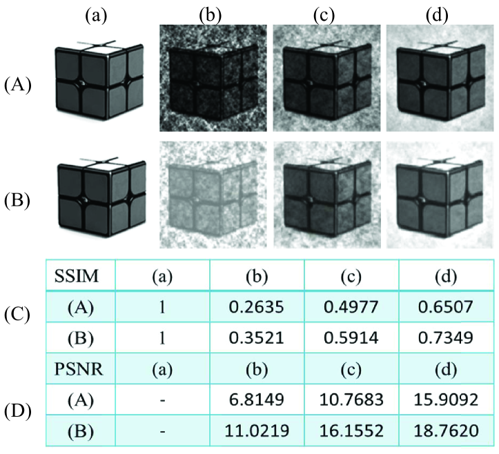
Figure 5: (A) The burred classical images caused by atmospheric turbulence, (B) Computational ghost images reconstructed by MsGAN method, (C) and (D) The SSIM and PSNR values of the images with different intensities of atmospheric turbulence. (a) classical images without atmospheric turbulence, (b), (c) and (d) show the burred images caused by different intensities of atmospheric turbulence.

In data processing, the superparameter of the loss function is set to $\alpha=0.5$, $\beta=0.01$, $\gamma=0.01$. Adam is used for parameter optimization in the training process, and batch_size is set to 1. In the data set, 173 and 35 real object images are collected as the training set and test set, respectively.

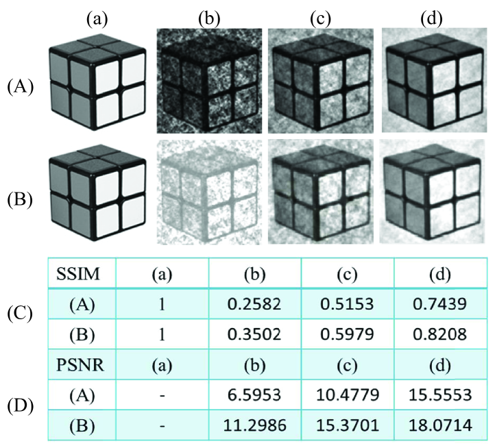
Figure 6: (A) The burred classical images caused by atmospheric turbulence, (B) Computational ghost images reconstructed by MsGAN method. SSIM and PSNR show that this method is effective for different objects, and the effect is almost the same.

The effect of turbulence on a classical image is easily observed in Figs. 5A(b-d), where three classical images were taken by a conventional CCD camera. Experimental results show that classical images are significantly blurred by turbulence. Moreover, with increasing turbulence intensity, the image distortion becomes more obvious. Figs. 5B(f-h) show the experimental results of this method. From the human vision, the reconstructed computational ghost images have better image quality than the turbulence blurred images and are similar to the images without turbulence. To quantitatively evaluate the effect of this method, we use the structural similarity (SSIM) and peak signal-to-noise ratio (PSNR) to measure the image quality. Figs. 5C and 5D show that the SSIM and PSNR of the reconstructed images are significantly better than the burred classical images. Indeed, SSIM and PSNR show that there is still a certain gap between the image obtained by this method and the complete turbulence-free image. However, from the perspective of human visual effect, the difference between the image obtained by this method and the turbulence-free image is acceptable. Consequently, this method is called turbulence-immune CGI. To prove the effectiveness of this method, we choose the other Rubik’s cubes as the object to experiment. The experimental results (Fig. 6) are almost identical to above one.

In summary, the first turbulence-immune computational ghost imaging experiment was demonstrated in this article. Although CGI framework does not satisfy the conditions of turbulence-free imaging, the satisfactory ghost image can be reconstructed using the MsGAN method in atmospheric turbulence environment. We hope that this method can provide a promising solution to overcome atmospheric turbulence in applications of CGI and single-pixel imaging.

National Natural Science Foundation of China (11704221, 11574178, 61675115), Taishan Scholar Project of Shandong Province (tsqn201812059).

The authors declare that there are no conflicts of interest related to this article.

Data underlying the results presented in this paper are not publicly available at this time but may be obtained from the authors upon reasonable request.

References

- (1) T. B. Pittman, Y. H. Shih, D. V. Strekalov, and A. V. Sergienko, Optical imaging by means of two-photon quantum entanglement, Phys. Rev. A 52, R3429 (1995).
- (2) D. Klyshko, Combine EPR and two-slit experiments: Interference of advanced waves, Phys. Lett. A 132, 299 (1988).
- (3) B. I. Erkmen and J. H. Shapiro, Ghost imaging: From quantum to classical to computational, Adv. Opt. Photon. 2, 405 (2010).
- (4) A. Valencia, G. Scarcelli, M. D’Angelo, and Y. Shih. Two-photon imaging with thermal light. Phys. Rev. Lett. 94, 063601 (2005).
- (5) R. S. Bennink, S. J. Bentley, and R. W. Boyd, Two-Photon Coincidence Imaging with a Classical Source, Phys. Rev. Lett. 89, 113601 (2002).
- (6) X. H. Chen, Q. Liu, K. H. Luo, L. A. Wu, Lensless ghost imaging with true thermal light, Opt. Lett. 34, 695-697 (2009).
- (7) J. H. Shapiro, Computational ghost imaging, Phys. Rev. A, 78, 061802(R) (2008).
- (8) Y. Bromberg, O. Katz, and Y. Silberberg, Ghost imaging with a single detector, Phys. Rev. A, 79, 053840 (2009).
- (9) B. I. Erkmen, Computational ghost imaging for remote sensing, J. Opt. Soc. Am A 29, 782-789, (2012).
- (10) M. Y. Chen, H. Wu, R. Z. Wang, Z. Y. He, H. Li, J. Q. Gan, G. P. Zhao, Computational ghost imaging with uncertain imaging distance, Opt. Commun. 445 (15) 106-110 (2019).
- (11) D. Y. Duan, Z. X. Man, and Y. J. Xia, Non-degenerate wavelength computational ghost imaging with thermal light, Opt. Express 27, 25187-25195 (2019).
- (12) N. D. Hardy and J. H. Shapiro, Computational ghost imaging versus imaging laser radar for three-dimensional imaging, Phys. Rev. A 87, 023820 (2013).
- (13) W. L. Gong, C. Q. Zhao, H. Yu, M. L. Chen, W. D. Xu, S. S. Han, Three-dimensional ghost imaging lidar via sparsity constraint, Sci. Rep. 6, 26133 (2016).
- (14) C. L. Wang, X. D. Mei, L. Pan, P. W. Wang, W. Li, X. Gao, Z. W. Bo, M. L. Chen, W. L. Gong S. S. Han, Airborne Near Infrared Three-Dimensional Ghost Imaging LiDAR via Sparsity Constraint, Remote Sens 10, 732 (2018).
- (15) W. L. Gong, H. Yu, C. Q. Zhao, Z. W. Bo, M . L. Chen, W. D. Xu, Improving the Imaging Quality of Ghost Imaging Lidar via Sparsity Constraint by Time-Resolved Technique, Remote Sens 8, 991 (2016).
- (16) C. J. Deng, L. Pan, C. L. Wang, X. Gao, W. L. Gong, and S. S. Han, Performance analysis of ghost imaging lidar in background light environment, Photon. Res. 5, 431-435 (2017).
- (17) H. C. Liu, S. Zhang, Computational ghost imaging of hot objects in long-wave infrared range, Appl. Phys. Lett. 111, 031110 (2017).
- (18) D. Y. Duan and Y. J. Xia, Pseudo color night vision correlated imaging without an infrared focal plane array, Opt. Express 29(4), 4978-4985 (2021).
- (19) R. E. Meyers, K. S. Deacon, and Y. Shih, Turbulence-free ghost imaging, Appl. Phys. Lett. 98(11), 111115 (2011).
- (20) R. E. Meyers, K. S. Deacon, and Y. H. Shi, Positive-negative turbulence-free ghost imaging, App. Phys. Lett. 100, 131114 (2012).
- (21) Y. H. Shih, The physics of turbulence-free ghost imaging, Technologies 4, 39 (2016).
- (22) Y. Shih, An Introduction to Quantum Optics: Photon and Biphoton Physics (Series in Optics and Optoelectronics), 1st ed. (Taylor & Francis, London, 2011).
- (23) M. F. Li, L. Yan, R. Yang, J. Kou, and Y. S. Liu, Turbulence-free intensity fluctuation self-correlation imaging with sunlight, Acta Phys. Sin. 68(9), 094204 (2019).
- (24) C. Zhen, Y. S. Yang, Y. X. Li, and J. J. Zhong, Atmospheric turbulence image restoration based on multi-scale generative adversarial network, Computer Engineering (to be published).
- (25) C. P. Lau, H. Souri, and R. Chellappa, ATFaceFAN: single face image restoration and recognition from atmospheric turbulence, arXiv:1910.03119 (2020).