Deep Learning Beam Optimization in
Millimeter-Wave Communication Systems

Abstract

We propose a method that combines fixed point algorithms with a neural network to optimize jointly discrete and continuous variables in millimeter-wave communication systems, so that the users’ rates are allocated fairly in a well-defined sense. In more detail, the discrete variables include user-access point assignments and the beam configurations, while the continuous variables refer to the power allocation. The beam configuration is predicted from user-related information using a neural network. Given the predicted beam configuration, a fixed point algorithm allocates power and assigns users to access points so that the users achieve the maximum fraction of their interference-free rates. The proposed method predicts the beam configuration in a “one-shot” manner, which significantly reduces the complexity of the beam search procedure. Moreover, even if the predicted beam configurations are not optimal, the fixed point algorithm still provides the optimal power allocation and user-access point assignments for the given beam configuration.

Index Terms—  Interference management, millimeter-wave communication, beamforming, deep learning, fixed point algorithm

1 Introduction

Communication over millimeter-wave (mmWave) bands is a key enabler to support increasing data rate demands [1]. Small wavelengths allow the exploitation of large antenna arrays in the current size of radio chips, which results in a substantial gain in the link budget using beamforming. Such a gain can largely compensate for the high path-loss in the mmWave band, without increasing the transmit power. Achieving higher gain, however, requires narrow beams both at the user equipment (UE) and at the access point (AP). The latter, in turn, needs to deal with difficult problems associated with the establishment and maintenance of a robust communication links with directional beams. Thus, resource management in mmWave systems becomes more difficult owing to additional system parameters such as beam width and beam direction, in comparison with conventional communication technologies with the omni- or semi-directional transmission. More specifically, in addition to the power allocation and UE-AP assignment problems in conventional communication systems, the network operating with directional beams further requires to find the optimal beam configurations to improve system performance with respect to network coverage, spectral efficiency, etc.

In practical mmWave communication systems, some transceivers are implemented with discrete beam configurations selected from a predefined finite set [2]. As a result, joint optimization of all discrete and continuous variables becomes difficult. For example, existing methods in the literature for power allocation [3, 4], beam configuration optimization [5, 6, 7] and UE-AP assignment [8, 9] cope with some of the continuous or the discrete variables, but the joint optimization of all these parameters is difficult and requires heuristics. For example, in a previous study [10], a method that jointly optimizes the transmit power of UEs, receive beam configurations of APs, and UE-AP assignments has been proposed. In that method, for fixed beam configurations of APs, the problem is formulated as a weighted rate allocation problem, where each UE maximizes the same portion of its maximum achievable rate that it would have in interference-free conditions. The solution to the aforementioned problem is obtained with an iterative fixed point algorithm that allocates power and assigns UEs to APs. However, the algorithm is unable to include the beam configurations in the optimization framework while guaranteeing optimality. As a result, the study in [10] combines fixed point algorithms with heuristics based on simulated annealing (SA) to cope with all optimization variables. Despite the high performance of the method in [10], from a practicality perspective, one of the challenges is to alleviate the complexity of the heuristic based on simulated annealing, which scales exponentially with the number of discrete beam configurations and the number of APs.

In this work, we propose a method that combines fixed point algorithms with a neural network, with the intent of jointly optimizing all discrete and continuous variables. To this end, we propose an architecture based on a deep neural network that is able to predict the beam configurations from UE related information. More precisely, we use a neural network for supervised multitask learning where each AP learns its best beam configuration in the sense of maximizing the common fraction of the maximum achievable rates of the UEs. Given the predicted beam configurations, the fixed point algorithm provides the solution for optimal transmit power allocation and the UE-AP assignments. With such a combination of a neural network with a fixed point algorithm, we have the following advantages. First, compared to the iterative SA, the neural network can predict the beam configuration in a “one-shot” manner, which results in a significant complexity reduction. Second, if the beam configurations produced by the neural network are suboptimal, then the fixed point algorithm is still optimal in the sense of maximizing the common fraction of interference-free rates for the given beam configurations. Third, with the settings considered here, the neural network can produce robust predictions under environmental changes (e.g., different distributions of UE positions).

2 System Model and Problem Statement

2.1 System Model

In this study, we use the following standard notations. By ${\left\|{\cdot}\right\|}_{\infty}$, we denote the standard $l-\infty$ norm. Sets of non-negative and strictly positive reals are denoted by $\mathbb{R}_{+}$ and $\mathbb{R}_{++}$, respectively.

We consider a wireless network with a set ${\mathcal{N}}={\left\{{1,...,N}\right\}}$ of transmitters, called UEs, and a set ${\mathcal{M}}={\left\{{1,...,M}\right\}}$ of receivers, called APs. The UE transmit beam configurations are denoted by ${\left({\forall n\in\mathcal{N}}\right)}\hskip 2.0pt\theta^{\text{Tx}}_{n}$ and $\beta^{\text{Tx}}_{n}$, where $\theta^{\text{Tx}}_{n}$ and $\beta^{\text{Tx}}_{n}$ are the $\text{UE}_{n}$ transmit beam width and direction, respectively. We assume that the transmit beam widths of UEs are identical and fixed ${\left({\forall n\in\mathcal{N}}\right)}\hskip 2.0pt\theta_{n}^{\text{Tx}}=\mkern 2.6mu\overline{\mkern-1.5mu\theta\mkern-1.5mu}\mkern 1.5mu^{\text{Tx}}$, while UE beam directions are uniformly distributed with ${\left({\forall n\in\mathcal{N}}\right)}\hskip 2.0pt\beta_{n}^{\text{Tx}}\sim\mathcal{U}{\left({\beta^{\text{Tx}}_{\text{min}},\beta^{\text{Tx}}_{\text{max}}}\right)}$. In contrast to the UEs, each AP beam width and direction can be adjusted by the respective AP, i.e. $\boldsymbol{\theta}^{\text{Rx}}={\left({\theta_{1}^{\text{Rx}},...,\theta_{M}^{\text{Rx}}}\right)}\in\mathbb{D}^{M}_{\theta}\subseteq\mathbb{R}^{M}_{++}$ and $\boldsymbol{\beta}^{\text{Rx}}={\left({\beta_{1}^{\text{Rx}},...,\beta_{M}^{\text{Rx}}}\right)}\in\mathbb{D}^{M}_{\beta}\subseteq\mathbb{R}^{M}$ are vectors to be optimized. Note that $\mathbb{D}_{\theta}$ and $\mathbb{D}_{\beta}$ denote the discrete sets of receive beam widths and directions, respectively. The transmit power vector of UEs is defined by ${\boldsymbol{p}}:={\left({p_{1},...,p_{N}}\right)}\in\mathbb{R}^{N}_{+}$, and the elements of this vector take values in the interval ${\left({\forall n\in\mathcal{N}}\right)}\hskip 2.0pt0<p_{n}\leq\mkern 2.6mu\overline{\mkern-1.5muP\mkern-1.5mu}\mkern 1.5mu$, where $\mkern 2.6mu\overline{\mkern-1.5muP\mkern-1.5mu}\mkern 1.5mu$ is the maximum allowed transmit power. In this work, we assume that multiple UEs may simultaneously connect to an AP.

For given ${\boldsymbol{p}},\boldsymbol{\theta}^{\text{Rx}}$, and $\boldsymbol{\beta}^{\text{Rx}}$, the achievable rate of UE _n in the uplink to its best serving AP (i.e. the UE-AP assignment) is expressed by

where $W$ is the system bandwidth, and

denotes the signal-to-interference-plus-noise ratio (SINR) for UE_n. The variable $\sigma^{2}>0$ is the noise power, and ${\left({\forall m\in\mathcal{M}}\right)}$ ${\left({\forall n\in\mathcal{N}}\right)}$ ${\left({\forall{\left({\boldsymbol{\theta}^{\text{Rx}},\boldsymbol{\beta}^{\text{Rx}}}\right)}\in\mathcal{Q}}\right)}$ $h_{m,n}{\left({\boldsymbol{\theta}^{\text{Rx}},\boldsymbol{\beta}^{\text{Rx}}}\right)}>0$ denotes the channel power gain between UE_n and serving AP_m given beam configuration ${\left({\boldsymbol{\theta}^{\text{Rx}},\boldsymbol{\beta}^{\text{Rx}}}\right)}\in\mathcal{Q}$, as defined in [10, Sect. II.C]. By fixing ${\left({\forall n\in\mathcal{N}}\right)}\hskip 2.0ptp_{n}=\mkern 2.6mu\overline{\mkern-1.5muP\mkern-1.5mu}\mkern 1.5mu$, the maximum achievable rate, also called interference-free rate, of UE _n is given by

$$\mkern 2.6mu\overline{\mkern-1.5muR\mkern-1.5mu}\mkern 1.5mu_{n}={\underset{m\in{\mathcal{M}},{\left({\boldsymbol{\theta}^{\text{Rx}},\boldsymbol{\beta}^{\text{Rx}}}\right)}\in\mathcal{Q}}{\text{max}}}W\log_{2}{\left({1+\dfrac{\mkern 2.6mu\overline{\mkern-1.5muP\mkern-1.5mu}\mkern 1.5muh_{m,n}{\left({\boldsymbol{\theta}^{\text{Rx}},\boldsymbol{\beta}^{\text{Rx}}}\right)}}{\sigma^{2}}}\right)}.$$ (3)

The rate $\mkern 2.6mu\overline{\mkern-1.5muR\mkern-1.5mu}\mkern 1.5mu_{n}$ corresponds to the case when UE _n transmits alone in the network with full power to its best serving AP.

2.2 Problem Statement

The problem in this study is defined as fair allocation of the UE rates ${\left({\forall n\in{\mathcal{N}}}\right)}\hskip 2.0ptR_{n}$, in the sense that every UE achieves the maximum common fraction $c\in{\left[{0,1}\right]}$ of its interference-free rates $\mkern 2.6mu\overline{\mkern-1.5muR\mkern-1.5mu}\mkern 1.5mu_{n}$. Formally, the optimization problem is stated as follows:

$$\underset{{\boldsymbol{p}},\boldsymbol{\theta}^{\text{Rx}},\boldsymbol{\beta}^{\text{Rx}},c}{\text{maximize}} \quad c$$ (4)

subject to $$\quad{\left({\forall n\in{\mathcal{N}}}\right)}\hskip 2.0ptc\mkern 2.6mu\overline{\mkern-1.5muR\mkern-1.5mu}\mkern 1.5mu_{n}=R_{n}{\left({{\boldsymbol{p}},\boldsymbol{\theta}^{\text{Rx}},\boldsymbol{\beta}^{\text{Rx}}}\right)}$$ (4a)

$$\quad{\left\|{{\boldsymbol{p}}}\right\|}_{\infty}\leq\mkern 2.6mu\overline{\mkern-1.5muP\mkern-1.5mu}\mkern 1.5mu$$ (4b)

$$\quad{\boldsymbol{p}}\in\mathbb{R}^{N}_{+},{\left({\boldsymbol{\theta}^{\text{Rx}},\boldsymbol{\beta}^{\text{Rx}}}\right)}\in{\mathcal{Q}},c\in\mathbb{R}_{++},$$ (4c)

where ${\mathcal{Q}}={\left\{{{\left({\boldsymbol{\theta}^{\text{Rx}}_{k},\boldsymbol{\beta}^{\text{Rx}}_{l}}\right)}}\right\}}_{k\in{\left({1,...,{\left|{\mathbb{D}_{\theta}}\right|}^{M}}\right)},\hskip 2.0ptl\in{\left({1,...,{\left|{\mathbb{D}_{\beta}}\right|}^{M}}\right)}}$ is a set of all receive beam configurations of the APs. The joint optimization of the parameters in (4) is challenging due to a mixture of discrete and continuous parameters.

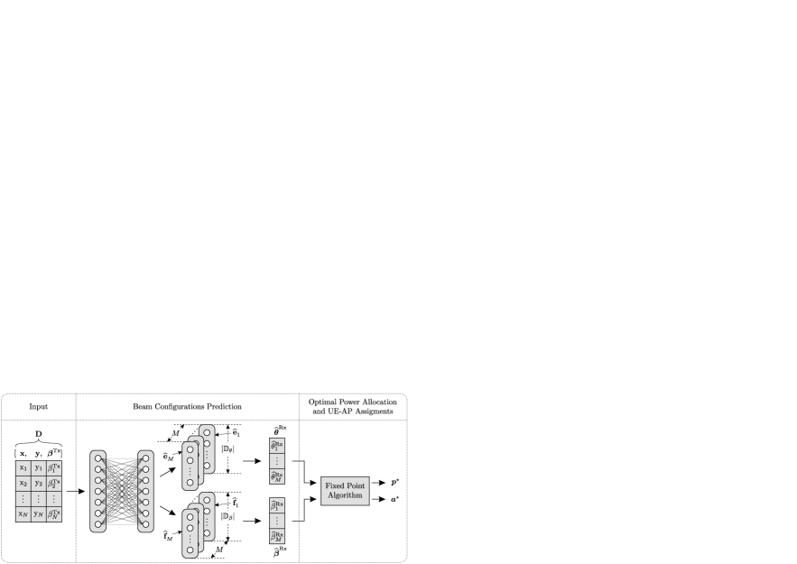
Fig. 1: The proposed architecture for joint optimization of the beam configurations, power allocation and UE-AP assignments. The neural network predicts the beam configurations from UE related information ${\mathbf{D}}$, and the fixed point algorithm optimally allocates the power and assigns the UEs to APs given the predicted beam configurations.

However, if the tuple ${\left({\boldsymbol{\theta}^{\text{Rx}},\boldsymbol{\beta}^{\text{Rx}}}\right)}$ is fixed to any given beam configuration ${\left({\mkern 2.6mu\overline{\mkern-1.5mu\boldsymbol{\theta}\mkern-1.5mu}\mkern 1.5mu^{\text{Rx}},\mkern 2.6mu\overline{\mkern-1.5mu\boldsymbol{\beta}\mkern-1.5mu}\mkern 1.5mu^{\text{Rx}}}\right)}\in{\mathcal{Q}}$, the objective reduces to the following power allocation and UE-AP assignment problem:

$$\underset{{\boldsymbol{p}},c}{\text{maximize}} \quad c$$ (5)

subject to $$\quad{\left({\forall n\in{\mathcal{N}}}\right)}\hskip 2.0ptc\mkern 2.6mu\overline{\mkern-1.5muR\mkern-1.5mu}\mkern 1.5mu_{n}=R_{n}{\left({{\boldsymbol{p}},\mkern 2.6mu\overline{\mkern-1.5mu\boldsymbol{\theta}\mkern-1.5mu}\mkern 1.5mu^{\text{Rx}},\mkern 2.6mu\overline{\mkern-1.5mu\boldsymbol{\beta}\mkern-1.5mu}\mkern 1.5mu^{\text{Rx}}}\right)},$$ (5a)

$$\quad{\left\|{{\boldsymbol{p}}}\right\|}_{\infty}\leq\mkern 2.6mu\overline{\mkern-1.5muP\mkern-1.5mu}\mkern 1.5mu$$ (5b)

$$\quad{\boldsymbol{p}}\in\mathbb{R}^{N}_{+},c\in\mathbb{R}_{++},$$ (5c)

and problem (5) can be solved optimally with a simple iterative fixed point algorithm [11][10, Sect. IV.A].

The connection between (4) and (5) can be summarized as follows. Suppose that ${\left({\mathchoice{\LMex=1ex\LMpt=1pt\ensurestackMath{\stackengine{1.0pt}{\hbox{$\SavedStyle\boldsymbol{\theta}$}}{\kern 1.24997pt\smash{\star}}{O}{c}{F}{T}{S}}}{\LMex=1ex\LMpt=1pt\ensurestackMath{\stackengine{1.0pt}{\hbox{$\SavedStyle\boldsymbol{\theta}$}}{\kern 1.24997pt\smash{\star}}{O}{c}{F}{T}{S}}}{\LMex=\scriptstyleScaleFactor ex\LMpt=\scriptstyleScaleFactor pt\ensurestackMath{\stackengine{1.0pt}{\hbox{$\SavedStyle\boldsymbol{\theta}$}}{\kern 1.24997pt\smash{\star}}{O}{c}{F}{T}{S}}}{\LMex=\scriptscriptstyleScaleFactor ex\LMpt=\scriptscriptstyleScaleFactor pt\ensurestackMath{\stackengine{1.0pt}{\hbox{$\SavedStyle\boldsymbol{\theta}$}}{\kern 1.24997pt\smash{\star}}{O}{c}{F}{T}{S}}}^{\text{Rx}},\mathchoice{\LMex=1ex\LMpt=1pt\ensurestackMath{\stackengine{1.0pt}{\hbox{$\SavedStyle\boldsymbol{\beta}$}}{\kern 1.24997pt\smash{\star}}{O}{c}{F}{T}{S}}}{\LMex=1ex\LMpt=1pt\ensurestackMath{\stackengine{1.0pt}{\hbox{$\SavedStyle\boldsymbol{\beta}$}}{\kern 1.24997pt\smash{\star}}{O}{c}{F}{T}{S}}}{\LMex=\scriptstyleScaleFactor ex\LMpt=\scriptstyleScaleFactor pt\ensurestackMath{\stackengine{1.0pt}{\hbox{$\SavedStyle\boldsymbol{\beta}$}}{\kern 1.24997pt\smash{\star}}{O}{c}{F}{T}{S}}}{\LMex=\scriptscriptstyleScaleFactor ex\LMpt=\scriptscriptstyleScaleFactor pt\ensurestackMath{\stackengine{1.0pt}{\hbox{$\SavedStyle\boldsymbol{\beta}$}}{\kern 1.24997pt\smash{\star}}{O}{c}{F}{T}{S}}}^{\text{Rx}}}\right)}\in{\mathcal{Q}}$ is an optimal beam configuration to problem (4). If we solve (5) by fixing $\mkern 2.6mu\overline{\mkern-1.5mu\boldsymbol{\theta}\mkern-1.5mu}\mkern 1.5mu^{\text{Rx}}=\mathchoice{\LMex=1ex\LMpt=1pt\ensurestackMath{\stackengine{1.0pt}{\hbox{$\SavedStyle\boldsymbol{\theta}$}}{\kern 1.24997pt\smash{\star}}{O}{c}{F}{T}{S}}}{\LMex=1ex\LMpt=1pt\ensurestackMath{\stackengine{1.0pt}{\hbox{$\SavedStyle\boldsymbol{\theta}$}}{\kern 1.24997pt\smash{\star}}{O}{c}{F}{T}{S}}}{\LMex=\scriptstyleScaleFactor ex\LMpt=\scriptstyleScaleFactor pt\ensurestackMath{\stackengine{1.0pt}{\hbox{$\SavedStyle\boldsymbol{\theta}$}}{\kern 1.24997pt\smash{\star}}{O}{c}{F}{T}{S}}}{\LMex=\scriptscriptstyleScaleFactor ex\LMpt=\scriptscriptstyleScaleFactor pt\ensurestackMath{\stackengine{1.0pt}{\hbox{$\SavedStyle\boldsymbol{\theta}$}}{\kern 1.24997pt\smash{\star}}{O}{c}{F}{T}{S}}}^{\text{Rx}}$ and $\mkern 2.6mu\overline{\mkern-1.5mu\boldsymbol{\beta}\mkern-1.5mu}\mkern 1.5mu^{\text{Rx}}=\mathchoice{\LMex=1ex\LMpt=1pt\ensurestackMath{\stackengine{1.0pt}{\hbox{$\SavedStyle\boldsymbol{\beta}$}}{\kern 1.24997pt\smash{\star}}{O}{c}{F}{T}{S}}}{\LMex=1ex\LMpt=1pt\ensurestackMath{\stackengine{1.0pt}{\hbox{$\SavedStyle\boldsymbol{\beta}$}}{\kern 1.24997pt\smash{\star}}{O}{c}{F}{T}{S}}}{\LMex=\scriptstyleScaleFactor ex\LMpt=\scriptstyleScaleFactor pt\ensurestackMath{\stackengine{1.0pt}{\hbox{$\SavedStyle\boldsymbol{\beta}$}}{\kern 1.24997pt\smash{\star}}{O}{c}{F}{T}{S}}}{\LMex=\scriptscriptstyleScaleFactor ex\LMpt=\scriptscriptstyleScaleFactor pt\ensurestackMath{\stackengine{1.0pt}{\hbox{$\SavedStyle\boldsymbol{\beta}$}}{\kern 1.24997pt\smash{\star}}{O}{c}{F}{T}{S}}}^{\text{Rx}}$, then the solution ${\left({c^{\star},{\boldsymbol{p}}^{\star}}\right)}$ to (5) is also the optimal fraction $c^{\star}$ and an optimal power allocation ${\boldsymbol{p}}^{\star}$ to problem (4). Furthermore, the entries of the optimal UE-AP assignment vector ${\boldsymbol{a}}^{\star}={\left({a_{1}^{\star},...,a_{N}^{\star}}\right)}\in\mathcal{M}\times\cdots\times\mathcal{M}$ can be recovered via

$$a^{\star}_{n}\in{\underset{m\in\mathcal{M}}{\text{arg min}}}\dfrac{\mkern 2.6mu\overline{\mkern-1.5muR\mkern-1.5mu}\mkern 1.5mu_{n}p^{\star}_{n}}{\vspace{10pt}W\log_{2}\Big{(}1+s_{n}{\left({{\boldsymbol{p}}^{\star},\mathchoice{\LMex=1ex\LMpt=1pt\ensurestackMath{\stackengine{1.0pt}{\hbox{$\SavedStyle\boldsymbol{\theta}$}}{\kern 1.24997pt\smash{\star}}{O}{c}{F}{T}{S}}}{\LMex=1ex\LMpt=1pt\ensurestackMath{\stackengine{1.0pt}{\hbox{$\SavedStyle\boldsymbol{\theta}$}}{\kern 1.24997pt\smash{\star}}{O}{c}{F}{T}{S}}}{\LMex=\scriptstyleScaleFactor ex\LMpt=\scriptstyleScaleFactor pt\ensurestackMath{\stackengine{1.0pt}{\hbox{$\SavedStyle\boldsymbol{\theta}$}}{\kern 1.24997pt\smash{\star}}{O}{c}{F}{T}{S}}}{\LMex=\scriptscriptstyleScaleFactor ex\LMpt=\scriptscriptstyleScaleFactor pt\ensurestackMath{\stackengine{1.0pt}{\hbox{$\SavedStyle\boldsymbol{\theta}$}}{\kern 1.24997pt\smash{\star}}{O}{c}{F}{T}{S}}}^{\text{Rx}},\mathchoice{\LMex=1ex\LMpt=1pt\ensurestackMath{\stackengine{1.0pt}{\hbox{$\SavedStyle\boldsymbol{\beta}$}}{\kern 1.24997pt\smash{\star}}{O}{c}{F}{T}{S}}}{\LMex=1ex\LMpt=1pt\ensurestackMath{\stackengine{1.0pt}{\hbox{$\SavedStyle\boldsymbol{\beta}$}}{\kern 1.24997pt\smash{\star}}{O}{c}{F}{T}{S}}}{\LMex=\scriptstyleScaleFactor ex\LMpt=\scriptstyleScaleFactor pt\ensurestackMath{\stackengine{1.0pt}{\hbox{$\SavedStyle\boldsymbol{\beta}$}}{\kern 1.24997pt\smash{\star}}{O}{c}{F}{T}{S}}}{\LMex=\scriptscriptstyleScaleFactor ex\LMpt=\scriptscriptstyleScaleFactor pt\ensurestackMath{\stackengine{1.0pt}{\hbox{$\SavedStyle\boldsymbol{\beta}$}}{\kern 1.24997pt\smash{\star}}{O}{c}{F}{T}{S}}}^{\text{Rx}},m}\right)}\Big{)}}.$$ (6)

Therefore, if the optimal beam configurations are known, (4) can be solved optimally with a simple fixed point algorithm. In principle, the optimal beam configurations could be found via exhaustive search or other iterative search methods (e.g. SA) over $\mathcal{Q}$, as done in [10]. Performing this search, however, scales exponentially with the number of discrete beam configurations and the number of APs. In the following, we propose a deep learning-based non-iterative method that predicts the beam configurations in a “one-shot” manner from UE related information.

3 Beam Configurations Prediction with Deep Neural Network

To find the optimal beam configuration ${\left({\mathchoice{\LMex=1ex\LMpt=1pt\ensurestackMath{\stackengine{1.0pt}{\hbox{$\SavedStyle\boldsymbol{\theta}$}}{\kern 1.24997pt\smash{\star}}{O}{c}{F}{T}{S}}}{\LMex=1ex\LMpt=1pt\ensurestackMath{\stackengine{1.0pt}{\hbox{$\SavedStyle\boldsymbol{\theta}$}}{\kern 1.24997pt\smash{\star}}{O}{c}{F}{T}{S}}}{\LMex=\scriptstyleScaleFactor ex\LMpt=\scriptstyleScaleFactor pt\ensurestackMath{\stackengine{1.0pt}{\hbox{$\SavedStyle\boldsymbol{\theta}$}}{\kern 1.24997pt\smash{\star}}{O}{c}{F}{T}{S}}}{\LMex=\scriptscriptstyleScaleFactor ex\LMpt=\scriptscriptstyleScaleFactor pt\ensurestackMath{\stackengine{1.0pt}{\hbox{$\SavedStyle\boldsymbol{\theta}$}}{\kern 1.24997pt\smash{\star}}{O}{c}{F}{T}{S}}}^{\text{Rx}},\mathchoice{\LMex=1ex\LMpt=1pt\ensurestackMath{\stackengine{1.0pt}{\hbox{$\SavedStyle\boldsymbol{\beta}$}}{\kern 1.24997pt\smash{\star}}{O}{c}{F}{T}{S}}}{\LMex=1ex\LMpt=1pt\ensurestackMath{\stackengine{1.0pt}{\hbox{$\SavedStyle\boldsymbol{\beta}$}}{\kern 1.24997pt\smash{\star}}{O}{c}{F}{T}{S}}}{\LMex=\scriptstyleScaleFactor ex\LMpt=\scriptstyleScaleFactor pt\ensurestackMath{\stackengine{1.0pt}{\hbox{$\SavedStyle\boldsymbol{\beta}$}}{\kern 1.24997pt\smash{\star}}{O}{c}{F}{T}{S}}}{\LMex=\scriptscriptstyleScaleFactor ex\LMpt=\scriptscriptstyleScaleFactor pt\ensurestackMath{\stackengine{1.0pt}{\hbox{$\SavedStyle\boldsymbol{\beta}$}}{\kern 1.24997pt\smash{\star}}{O}{c}{F}{T}{S}}}^{\text{Rx}}}\right)}$ in (4), we assume that there exists an ideal mapping $\Xi$ that maps the UE related information ${\mathbf{D}}$ to some output $\big{(}{\left[{{\mathbf{e}}_{1}^{\star},..,{\mathbf{e}}_{M}^{\star}}\right]},{\left[{{\mathbf{f}}_{1}^{\star},..,{\mathbf{f}}_{M}^{\star}}\right]}\big{)}$ (to be explained later) such that $\mathchoice{\LMex=1ex\LMpt=1pt\ensurestackMath{\stackengine{1.0pt}{\hbox{$\SavedStyle\boldsymbol{\theta}$}}{\kern 1.24997pt\smash{\star}}{O}{c}{F}{T}{S}}}{\LMex=1ex\LMpt=1pt\ensurestackMath{\stackengine{1.0pt}{\hbox{$\SavedStyle\boldsymbol{\theta}$}}{\kern 1.24997pt\smash{\star}}{O}{c}{F}{T}{S}}}{\LMex=\scriptstyleScaleFactor ex\LMpt=\scriptstyleScaleFactor pt\ensurestackMath{\stackengine{1.0pt}{\hbox{$\SavedStyle\boldsymbol{\theta}$}}{\kern 1.24997pt\smash{\star}}{O}{c}{F}{T}{S}}}{\LMex=\scriptscriptstyleScaleFactor ex\LMpt=\scriptscriptstyleScaleFactor pt\ensurestackMath{\stackengine{1.0pt}{\hbox{$\SavedStyle\boldsymbol{\theta}$}}{\kern 1.24997pt\smash{\star}}{O}{c}{F}{T}{S}}}^{\text{Rx}}$ and $\mathchoice{\LMex=1ex\LMpt=1pt\ensurestackMath{\stackengine{1.0pt}{\hbox{$\SavedStyle\boldsymbol{\beta}$}}{\kern 1.24997pt\smash{\star}}{O}{c}{F}{T}{S}}}{\LMex=1ex\LMpt=1pt\ensurestackMath{\stackengine{1.0pt}{\hbox{$\SavedStyle\boldsymbol{\beta}$}}{\kern 1.24997pt\smash{\star}}{O}{c}{F}{T}{S}}}{\LMex=\scriptstyleScaleFactor ex\LMpt=\scriptstyleScaleFactor pt\ensurestackMath{\stackengine{1.0pt}{\hbox{$\SavedStyle\boldsymbol{\beta}$}}{\kern 1.24997pt\smash{\star}}{O}{c}{F}{T}{S}}}{\LMex=\scriptscriptstyleScaleFactor ex\LMpt=\scriptscriptstyleScaleFactor pt\ensurestackMath{\stackengine{1.0pt}{\hbox{$\SavedStyle\boldsymbol{\beta}$}}{\kern 1.24997pt\smash{\star}}{O}{c}{F}{T}{S}}}^{\text{Rx}}$ can be reconstructed from ${\left[{{\mathbf{e}}_{1}^{\star},..,{\mathbf{e}}_{M}^{\star}}\right]}$ and ${\left[{{\mathbf{f}}_{1}^{\star},..,{\mathbf{f}}_{M}^{\star}}\right]}$, respectively, and the reconstructed configuration ${\left({\mathchoice{\LMex=1ex\LMpt=1pt\ensurestackMath{\stackengine{1.0pt}{\hbox{$\SavedStyle\boldsymbol{\theta}$}}{\kern 1.24997pt\smash{\star}}{O}{c}{F}{T}{S}}}{\LMex=1ex\LMpt=1pt\ensurestackMath{\stackengine{1.0pt}{\hbox{$\SavedStyle\boldsymbol{\theta}$}}{\kern 1.24997pt\smash{\star}}{O}{c}{F}{T}{S}}}{\LMex=\scriptstyleScaleFactor ex\LMpt=\scriptstyleScaleFactor pt\ensurestackMath{\stackengine{1.0pt}{\hbox{$\SavedStyle\boldsymbol{\theta}$}}{\kern 1.24997pt\smash{\star}}{O}{c}{F}{T}{S}}}{\LMex=\scriptscriptstyleScaleFactor ex\LMpt=\scriptscriptstyleScaleFactor pt\ensurestackMath{\stackengine{1.0pt}{\hbox{$\SavedStyle\boldsymbol{\theta}$}}{\kern 1.24997pt\smash{\star}}{O}{c}{F}{T}{S}}}^{\text{Rx}},\mathchoice{\LMex=1ex\LMpt=1pt\ensurestackMath{\stackengine{1.0pt}{\hbox{$\SavedStyle\boldsymbol{\beta}$}}{\kern 1.24997pt\smash{\star}}{O}{c}{F}{T}{S}}}{\LMex=1ex\LMpt=1pt\ensurestackMath{\stackengine{1.0pt}{\hbox{$\SavedStyle\boldsymbol{\beta}$}}{\kern 1.24997pt\smash{\star}}{O}{c}{F}{T}{S}}}{\LMex=\scriptstyleScaleFactor ex\LMpt=\scriptstyleScaleFactor pt\ensurestackMath{\stackengine{1.0pt}{\hbox{$\SavedStyle\boldsymbol{\beta}$}}{\kern 1.24997pt\smash{\star}}{O}{c}{F}{T}{S}}}{\LMex=\scriptscriptstyleScaleFactor ex\LMpt=\scriptscriptstyleScaleFactor pt\ensurestackMath{\stackengine{1.0pt}{\hbox{$\SavedStyle\boldsymbol{\beta}$}}{\kern 1.24997pt\smash{\star}}{O}{c}{F}{T}{S}}}^{\text{Rx}}}\right)}$ is the optimal beam configuration to problem (4). Formally, the ideal mapping $\Xi$ is defined as follows

where ${\mathbf{D}}={\left[{{\mathbf{x}},{\mathbf{y}},\boldsymbol{\beta}^{\text{Tx}}}\right]}$ is the matrix that contains UE location information in a 2D Cartesian coordinate system ${\left[{{\mathbf{x}},{\mathbf{y}}}\right]}$, and $\boldsymbol{\beta}^{\text{Tx}}$ is the UE beam direction. The rows of the matrix ${\mathbf{D}}$ are sorted in lexicographical order.

We now proceed to explain the output of the ideal mapping $\Xi$, and we also describe the reconstruction mechanism to obtain $\mathchoice{\LMex=1ex\LMpt=1pt\ensurestackMath{\stackengine{1.0pt}{\hbox{$\SavedStyle\boldsymbol{\theta}$}}{\kern 1.24997pt\smash{\star}}{O}{c}{F}{T}{S}}}{\LMex=1ex\LMpt=1pt\ensurestackMath{\stackengine{1.0pt}{\hbox{$\SavedStyle\boldsymbol{\theta}$}}{\kern 1.24997pt\smash{\star}}{O}{c}{F}{T}{S}}}{\LMex=\scriptstyleScaleFactor ex\LMpt=\scriptstyleScaleFactor pt\ensurestackMath{\stackengine{1.0pt}{\hbox{$\SavedStyle\boldsymbol{\theta}$}}{\kern 1.24997pt\smash{\star}}{O}{c}{F}{T}{S}}}{\LMex=\scriptscriptstyleScaleFactor ex\LMpt=\scriptscriptstyleScaleFactor pt\ensurestackMath{\stackengine{1.0pt}{\hbox{$\SavedStyle\boldsymbol{\theta}$}}{\kern 1.24997pt\smash{\star}}{O}{c}{F}{T}{S}}}^{\text{Rx}}$ and $\mathchoice{\LMex=1ex\LMpt=1pt\ensurestackMath{\stackengine{1.0pt}{\hbox{$\SavedStyle\boldsymbol{\beta}$}}{\kern 1.24997pt\smash{\star}}{O}{c}{F}{T}{S}}}{\LMex=1ex\LMpt=1pt\ensurestackMath{\stackengine{1.0pt}{\hbox{$\SavedStyle\boldsymbol{\beta}$}}{\kern 1.24997pt\smash{\star}}{O}{c}{F}{T}{S}}}{\LMex=\scriptstyleScaleFactor ex\LMpt=\scriptstyleScaleFactor pt\ensurestackMath{\stackengine{1.0pt}{\hbox{$\SavedStyle\boldsymbol{\beta}$}}{\kern 1.24997pt\smash{\star}}{O}{c}{F}{T}{S}}}{\LMex=\scriptscriptstyleScaleFactor ex\LMpt=\scriptscriptstyleScaleFactor pt\ensurestackMath{\stackengine{1.0pt}{\hbox{$\SavedStyle\boldsymbol{\beta}$}}{\kern 1.24997pt\smash{\star}}{O}{c}{F}{T}{S}}}^{\text{Rx}}$ from ${\left[{{\mathbf{e}}_{1}^{\star},..,{\mathbf{e}}_{M}^{\star}}\right]}$ and ${\left[{{\mathbf{f}}_{1}^{\star},..,{\mathbf{f}}_{M}^{\star}}\right]}$. We assume that the elements of the vectors ${\left({\forall m\in\mathcal{M}}\right)}\hskip 2.0pt{\mathbf{e}}^{\star}_{m},{\mathbf{f}}^{\star}_{m}$ are one-hot encoded, i.e., ${\left({\forall m\in\mathcal{M}}\right)}\hskip 2.0pt{\mathbf{e}}^{\star}_{m}\in{\left\{{0,1}\right\}}^{|\mathbb{D}_{\theta}|},{\mathbf{f}}^{\star}_{m}\in{\left\{{0,1}\right\}}^{|\mathbb{D}_{\beta}|}$. In this way, the indices of the vectors ${\left({\forall m\in\mathcal{M}}\right)}\hskip 2.0pt{\mathbf{e}}_{m}^{\star},{\mathbf{f}}_{m}^{\star}$ are associated with the indices of the respective beam width and direction indices from the discrete sets $\mathbb{D}_{\theta}$ and $\mathbb{D}_{\beta}$. To relate the selected optimal beam indices (in the sense of maximizing the objective in (4)), we further assume that the vectors ${\left({\forall m\in\mathcal{M}}\right)}\hskip 2.0pt{\mathbf{e}}_{m}^{\star},{\mathbf{f}}_{m}^{\star}$ contain the value one at the index corresponding to the selected optimal beam width and direction, respectively, and zeros elsewhere.

With the output explained above, the reconstruction of the beam configurations $\mathchoice{\LMex=1ex\LMpt=1pt\ensurestackMath{\stackengine{1.0pt}{\hbox{$\SavedStyle\boldsymbol{\theta}$}}{\kern 1.24997pt\smash{\star}}{O}{c}{F}{T}{S}}}{\LMex=1ex\LMpt=1pt\ensurestackMath{\stackengine{1.0pt}{\hbox{$\SavedStyle\boldsymbol{\theta}$}}{\kern 1.24997pt\smash{\star}}{O}{c}{F}{T}{S}}}{\LMex=\scriptstyleScaleFactor ex\LMpt=\scriptstyleScaleFactor pt\ensurestackMath{\stackengine{1.0pt}{\hbox{$\SavedStyle\boldsymbol{\theta}$}}{\kern 1.24997pt\smash{\star}}{O}{c}{F}{T}{S}}}{\LMex=\scriptscriptstyleScaleFactor ex\LMpt=\scriptscriptstyleScaleFactor pt\ensurestackMath{\stackengine{1.0pt}{\hbox{$\SavedStyle\boldsymbol{\theta}$}}{\kern 1.24997pt\smash{\star}}{O}{c}{F}{T}{S}}}^{\text{Rx}}$ and $\mathchoice{\LMex=1ex\LMpt=1pt\ensurestackMath{\stackengine{1.0pt}{\hbox{$\SavedStyle\boldsymbol{\beta}$}}{\kern 1.24997pt\smash{\star}}{O}{c}{F}{T}{S}}}{\LMex=1ex\LMpt=1pt\ensurestackMath{\stackengine{1.0pt}{\hbox{$\SavedStyle\boldsymbol{\beta}$}}{\kern 1.24997pt\smash{\star}}{O}{c}{F}{T}{S}}}{\LMex=\scriptstyleScaleFactor ex\LMpt=\scriptstyleScaleFactor pt\ensurestackMath{\stackengine{1.0pt}{\hbox{$\SavedStyle\boldsymbol{\beta}$}}{\kern 1.24997pt\smash{\star}}{O}{c}{F}{T}{S}}}{\LMex=\scriptscriptstyleScaleFactor ex\LMpt=\scriptscriptstyleScaleFactor pt\ensurestackMath{\stackengine{1.0pt}{\hbox{$\SavedStyle\boldsymbol{\beta}$}}{\kern 1.24997pt\smash{\star}}{O}{c}{F}{T}{S}}}^{\text{Rx}}$ is performed as follows. Once we obtain the output $\big{(}{\left[{{\mathbf{e}}_{1}^{\star},..,{\mathbf{e}}_{M}^{\star}}\right]},{\left[{{\mathbf{f}}_{1}^{\star},..,{\mathbf{f}}_{M}^{\star}}\right]}\big{)}$ from $\Xi$, the vectors $\mathchoice{\LMex=1ex\LMpt=1pt\ensurestackMath{\stackengine{1.0pt}{\hbox{$\SavedStyle\boldsymbol{\theta}$}}{\kern 1.24997pt\smash{\star}}{O}{c}{F}{T}{S}}}{\LMex=1ex\LMpt=1pt\ensurestackMath{\stackengine{1.0pt}{\hbox{$\SavedStyle\boldsymbol{\theta}$}}{\kern 1.24997pt\smash{\star}}{O}{c}{F}{T}{S}}}{\LMex=\scriptstyleScaleFactor ex\LMpt=\scriptstyleScaleFactor pt\ensurestackMath{\stackengine{1.0pt}{\hbox{$\SavedStyle\boldsymbol{\theta}$}}{\kern 1.24997pt\smash{\star}}{O}{c}{F}{T}{S}}}{\LMex=\scriptscriptstyleScaleFactor ex\LMpt=\scriptscriptstyleScaleFactor pt\ensurestackMath{\stackengine{1.0pt}{\hbox{$\SavedStyle\boldsymbol{\theta}$}}{\kern 1.24997pt\smash{\star}}{O}{c}{F}{T}{S}}}^{\text{Rx}}$ and $\mathchoice{\LMex=1ex\LMpt=1pt\ensurestackMath{\stackengine{1.0pt}{\hbox{$\SavedStyle\boldsymbol{\beta}$}}{\kern 1.24997pt\smash{\star}}{O}{c}{F}{T}{S}}}{\LMex=1ex\LMpt=1pt\ensurestackMath{\stackengine{1.0pt}{\hbox{$\SavedStyle\boldsymbol{\beta}$}}{\kern 1.24997pt\smash{\star}}{O}{c}{F}{T}{S}}}{\LMex=\scriptstyleScaleFactor ex\LMpt=\scriptstyleScaleFactor pt\ensurestackMath{\stackengine{1.0pt}{\hbox{$\SavedStyle\boldsymbol{\beta}$}}{\kern 1.24997pt\smash{\star}}{O}{c}{F}{T}{S}}}{\LMex=\scriptscriptstyleScaleFactor ex\LMpt=\scriptscriptstyleScaleFactor pt\ensurestackMath{\stackengine{1.0pt}{\hbox{$\SavedStyle\boldsymbol{\beta}$}}{\kern 1.24997pt\smash{\star}}{O}{c}{F}{T}{S}}}^{\text{Rx}}$ are recovered via

$$\mathchoice{\LMex=1ex\LMpt=1pt\ensurestackMath{\stackengine{1.0pt}{\hbox{$\SavedStyle\boldsymbol{\theta}$}}{\kern 1.24997pt\smash{\star}}{O}{c}{F}{T}{S}}}{\LMex=1ex\LMpt=1pt\ensurestackMath{\stackengine{1.0pt}{\hbox{$\SavedStyle\boldsymbol{\theta}$}}{\kern 1.24997pt\smash{\star}}{O}{c}{F}{T}{S}}}{\LMex=\scriptstyleScaleFactor ex\LMpt=\scriptstyleScaleFactor pt\ensurestackMath{\stackengine{1.0pt}{\hbox{$\SavedStyle\boldsymbol{\theta}$}}{\kern 1.24997pt\smash{\star}}{O}{c}{F}{T}{S}}}{\LMex=\scriptscriptstyleScaleFactor ex\LMpt=\scriptscriptstyleScaleFactor pt\ensurestackMath{\stackengine{1.0pt}{\hbox{$\SavedStyle\boldsymbol{\theta}$}}{\kern 1.24997pt\smash{\star}}{O}{c}{F}{T}{S}}}^{\text{Rx}}={\left({\mathchoice{\LMex=1ex\LMpt=1pt\ensurestackMath{\stackengine{1.0pt}{\hbox{$\SavedStyle\theta$}}{\kern 1.24997pt\smash{\star}}{O}{c}{F}{T}{S}}}{\LMex=1ex\LMpt=1pt\ensurestackMath{\stackengine{1.0pt}{\hbox{$\SavedStyle\theta$}}{\kern 1.24997pt\smash{\star}}{O}{c}{F}{T}{S}}}{\LMex=\scriptstyleScaleFactor ex\LMpt=\scriptstyleScaleFactor pt\ensurestackMath{\stackengine{1.0pt}{\hbox{$\SavedStyle\theta$}}{\kern 1.24997pt\smash{\star}}{O}{c}{F}{T}{S}}}{\LMex=\scriptscriptstyleScaleFactor ex\LMpt=\scriptscriptstyleScaleFactor pt\ensurestackMath{\stackengine{1.0pt}{\hbox{$\SavedStyle\theta$}}{\kern 1.24997pt\smash{\star}}{O}{c}{F}{T}{S}}}^{\text{Rx}}_{1},...,\mathchoice{\LMex=1ex\LMpt=1pt\ensurestackMath{\stackengine{1.0pt}{\hbox{$\SavedStyle\theta$}}{\kern 1.24997pt\smash{\star}}{O}{c}{F}{T}{S}}}{\LMex=1ex\LMpt=1pt\ensurestackMath{\stackengine{1.0pt}{\hbox{$\SavedStyle\theta$}}{\kern 1.24997pt\smash{\star}}{O}{c}{F}{T}{S}}}{\LMex=\scriptstyleScaleFactor ex\LMpt=\scriptstyleScaleFactor pt\ensurestackMath{\stackengine{1.0pt}{\hbox{$\SavedStyle\theta$}}{\kern 1.24997pt\smash{\star}}{O}{c}{F}{T}{S}}}{\LMex=\scriptscriptstyleScaleFactor ex\LMpt=\scriptscriptstyleScaleFactor pt\ensurestackMath{\stackengine{1.0pt}{\hbox{$\SavedStyle\theta$}}{\kern 1.24997pt\smash{\star}}{O}{c}{F}{T}{S}}}^{\text{Rx}}_{M}}\right)},{\left({\forall m\in\mathcal{M}}\right)}\begin{array}[]{l}\mathchoice{\LMex=1ex\LMpt=1pt\ensurestackMath{\stackengine{1.0pt}{\hbox{$\SavedStyle\theta$}}{\kern 1.24997pt\smash{\star}}{O}{c}{F}{T}{S}}}{\LMex=1ex\LMpt=1pt\ensurestackMath{\stackengine{1.0pt}{\hbox{$\SavedStyle\theta$}}{\kern 1.24997pt\smash{\star}}{O}{c}{F}{T}{S}}}{\LMex=\scriptstyleScaleFactor ex\LMpt=\scriptstyleScaleFactor pt\ensurestackMath{\stackengine{1.0pt}{\hbox{$\SavedStyle\theta$}}{\kern 1.24997pt\smash{\star}}{O}{c}{F}{T}{S}}}{\LMex=\scriptscriptstyleScaleFactor ex\LMpt=\scriptscriptstyleScaleFactor pt\ensurestackMath{\stackengine{1.0pt}{\hbox{$\SavedStyle\theta$}}{\kern 1.24997pt\smash{\star}}{O}{c}{F}{T}{S}}}_{m}^{\text{Rx}}=\gamma_{i^{\star}_{m}}\in\mathbb{D}_{\theta}\\ i^{\star}_{m}\in{\underset{i=1,...,|\mathbb{D}_{\theta}|}{\text{arg max}}}{\left({{\left[{{\mathbf{e}}^{\star}_{m}}\right]}_{i}}\right)}\end{array}$$ (8)

and

where $\gamma_{i^{\star}_{m}}$ and $\delta_{i^{\star}_{m}}$ represent the selected optimal beam configurations from the finite and discrete sets $\mathbb{D}_{\theta}$ and $\mathbb{D}_{\beta}$, respectively. Although the ideal mapping $\Xi$ provides optimal beam configurations by assumption, it is challenging to analytically characterize it. Therefore we propose a deep neural network that learns an ideal mapping $\Xi$ from data.

The proposed neural network architecture in combination with the fixed point algorithm is shown in Fig. 1. With the setting that the beam configurations are taken from the discrete and finite sets $\mathbb{D}_{\theta}$ and $\mathbb{D}_{\beta}$, we consider the beam configurations as labels, and we pose the beam optimization problem in (4) as a multi-label classification problem [12]. The labels are constructed as follows. Given the finite set $\mathcal{Q}$ consisting of all possible beam configurations, and the UE related information ${\mathbf{D}}$, we perform an exhaustive search by applying fixed point iterations for every candidate beam configuration ${\left({\boldsymbol{\theta}^{\text{Rx}},\boldsymbol{\beta}^{\text{Rx}}}\right)}\in{\mathcal{Q}}$ to obtain ${\left({\mathchoice{\LMex=1ex\LMpt=1pt\ensurestackMath{\stackengine{1.0pt}{\hbox{$\SavedStyle\boldsymbol{\theta}$}}{\kern 1.24997pt\smash{\star}}{O}{c}{F}{T}{S}}}{\LMex=1ex\LMpt=1pt\ensurestackMath{\stackengine{1.0pt}{\hbox{$\SavedStyle\boldsymbol{\theta}$}}{\kern 1.24997pt\smash{\star}}{O}{c}{F}{T}{S}}}{\LMex=\scriptstyleScaleFactor ex\LMpt=\scriptstyleScaleFactor pt\ensurestackMath{\stackengine{1.0pt}{\hbox{$\SavedStyle\boldsymbol{\theta}$}}{\kern 1.24997pt\smash{\star}}{O}{c}{F}{T}{S}}}{\LMex=\scriptscriptstyleScaleFactor ex\LMpt=\scriptscriptstyleScaleFactor pt\ensurestackMath{\stackengine{1.0pt}{\hbox{$\SavedStyle\boldsymbol{\theta}$}}{\kern 1.24997pt\smash{\star}}{O}{c}{F}{T}{S}}}^{\text{Rx}},\mathchoice{\LMex=1ex\LMpt=1pt\ensurestackMath{\stackengine{1.0pt}{\hbox{$\SavedStyle\boldsymbol{\beta}$}}{\kern 1.24997pt\smash{\star}}{O}{c}{F}{T}{S}}}{\LMex=1ex\LMpt=1pt\ensurestackMath{\stackengine{1.0pt}{\hbox{$\SavedStyle\boldsymbol{\beta}$}}{\kern 1.24997pt\smash{\star}}{O}{c}{F}{T}{S}}}{\LMex=\scriptstyleScaleFactor ex\LMpt=\scriptstyleScaleFactor pt\ensurestackMath{\stackengine{1.0pt}{\hbox{$\SavedStyle\boldsymbol{\beta}$}}{\kern 1.24997pt\smash{\star}}{O}{c}{F}{T}{S}}}{\LMex=\scriptscriptstyleScaleFactor ex\LMpt=\scriptscriptstyleScaleFactor pt\ensurestackMath{\stackengine{1.0pt}{\hbox{$\SavedStyle\boldsymbol{\beta}$}}{\kern 1.24997pt\smash{\star}}{O}{c}{F}{T}{S}}}^{\text{Rx}}}\right)}$. Next, we retrieve ${\left({m\in\mathcal{M}}\right)}\hskip 2.0pti^{\star}_{m}$ by following the rules in (8) and (9). With the optimal index $i^{\star}_{m}$ we construct the one-hot encoded ground truth labels $\big{(}{\left[{{\mathbf{e}}_{1}^{\star},..,{\mathbf{e}}_{M}^{\star}}\right]},{\left[{{\mathbf{f}}_{1}^{\star},..,{\mathbf{f}}_{M}^{\star}}\right]}\big{)}$.

Given the input-output pair $\Big{(}{\mathbf{D}},\big{(}{\left[{{\mathbf{e}}_{1}^{\star},..,{\mathbf{e}}_{M}^{\star}}\right]},{\left[{{\mathbf{f}}_{1}^{\star},..,{\mathbf{f}}_{M}^{\star}}\right]}\big{)}\Big{)}$, we extract the features from ${\mathbf{D}}$ by utilizing two fully connected layers with the rectified linear unit (ReLU) activation as illustrated in Fig. 1. To project the extracted features onto beam configuration labels, we customize the multi-label classification layer with the softmax activation function so that ${\left({\forall m\in\mathcal{M}}\right)}\hskip 2.0pt\widehat{{\mathbf{e}}}_{m}\in{\left[{0,1}\right]}^{|\mathbb{D}_{\theta}|}$ and $\widehat{{\mathbf{f}}}_{m}\in{\left[{0,1}\right]}^{|\mathbb{D}_{\beta}|}$. With this design, the output of the neural network indicates the beam configuration indices. In other words, the indices of the highest values in ${\left({\forall m\in\mathcal{M}}\right)}\hskip 2.0pt\widehat{{\mathbf{e}}}_{m},\widehat{{\mathbf{f}}}_{m}$ indicates the best predicted beam width and direction for AP_m. We train the neural network by trying to minimize the categorical cross entropy loss [13] given by

4 Numerical Results

4.1 Training Parameters and Reference Methods

To train the proposed neural network, we generate $10^{6}$ samples, and we split those samples into training and test sets containing $9\cdot 10^{5}$ and $1\cdot 10^{5}$ samples, respectively. The samples are generated using the mmWave channel model described in [14]. The channel model considers an urban microcell (UMi)- line-of-sight (LoS) scenario with high user density in open areas and street canyons. The neural network has two hidden layers, each consisting of 200 fully connected neurons. The total number of epochs and batch size for training is 500 and 512, respectively. We train a neural network using the Adadelta optimizer [15] with adaptive learning rates.

We compare the performance of the proposed method with exhaustive search and with the method in [10]. In addition, we also introduce a method called naive learning. It simply provides to the fixed point algorithm the beam configurations encountered most frequently in the training set.

4.2 Simulation

Performing an exhaustive search over a large solution set $\mathcal{Q}$ is infeasible, so, for the simulations, we consider a small scale problem with $N=10$ UEs, $M=3$ APs, discrete receive beam width configurations $\mathbb{D}_{\theta}={\left\{{30^{\circ},45^{\circ},60^{\circ}}\right\}}$ and discrete receive beam direction configurations $\mathbb{D}_{\beta}={\left\{{80^{\circ},90^{\circ},100^{\circ}}\right\}}$. The UEs are located in a $20\times 30$ m² rectangle area centered at ${\left[{0\text{m},0\text{m}}\right]}$. With the given parameters, the size of the solution set is ${\left|{{\mathcal{Q}}}\right|}={\left|{\mathbb{D}_{\theta}}\right|}^{M}\times{\left|{\mathbb{D}_{\beta}}\right|}^{M}=729$. We set the number of fixed point iterations to 100. The heuristic based on simulated annealing proposed in [10] selects the initial beam configurations from the solution set ${\mathcal{Q}}$ uniformly at random, without prior knowledge about the configuration of the mmWave network. We formally define the optimal rate fraction $c^{\star}$ obtained by exhaustive as 100 % solution efficiency, and we compare the relative performances of other methods with the optimal solution obtained by exhaustive search. To evaluate the robustness of the proposed neural network against distribution changes in the input data, we consider the following two cases:

• The UE positions ${\left[{{\mathbf{x}},{\mathbf{y}}}\right]}$ in ${\mathbf{D}}$ are selected randomly from a uniform distribution within the rectangle area for both training and testing.

• The UE positions ${\left[{{\mathbf{x}},{\mathbf{y}}}\right]}$ in ${\mathbf{D}}$ are selected randomly from a uniform distribution within the rectangle area only for the training set. The UE positions ${\left[{{\mathbf{x}},{\mathbf{y}}}\right]}$ in the test set is selected randomly from a non-uniform distribution within the rectangle area. More precisely, we consider two uniformly distributed random variables $r\in[0,L]$ and $\phi\in[0,2\pi]$, where $L$ denotes the radius of a disk, and we generate the UE coordinates $[\text{x},\text{y}]$ in 2D Cartesian coordinate system as

  $$\text{x}=\text{x}_{\text{center}}+r\cos\phi\hskip 5.0pt\text{and}\hskip 5.0pt\text{y}=\text{y}_{\text{center}}+r\sin\phi,$$ (11)

  where $\text{x}_{\text{center}}$ and $\text{y}_{\text{center}}$ denote the center of a disk on $X$ and $Y$ axis, respectively. A scatter plot obtained with this distribution is illustrated in Fig. 2. Note that only the UE positions within the rectangle area were used for the simulation as shown in Fig. 2.

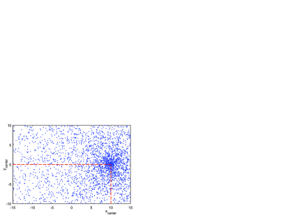
Fig. 2: Sample scatter plot of UE positions in the test set.

The performance of the proposed and reference methods are given in Fig. 3. The superscripts ${}^{\text{C1}}$ and ${}^{\text{C2}}$ in Fig. 3 denote the performance of the neural network and the naive learning approaches according to the previously-mentioned cases. Since all methods other than the simulated annealing and the exhaustive search method are predicting the beam configurations in a “one-shot” manner, we mark their performance with points, and we extend the dashed lines with the respective solution efficiency values in the X-axis.

In Fig. 3, we notice a substantial gap between the performance of the neural network and the naive learning approach under C1. This result shows that the neural network is able to predict good beam configurations from UE related information. The second, and very attractive result in Fig. 3, is the similar performance of the neural network under C2 and C1. This result indicates that the distribution used for training is likely to provide good performance when the distribution of the test set differs. In addition, we note that the proposed scheme requires only a single call to a fixed point algorithm (100 iterations are used) to achieve 80 % of the optimal rates on average. In contrast, the approach in [10] and exaustive search require one call to the fixed point algorithm for each configuration being probed. As a result, the number of iterations of the fixed point algorithm required by those heuristics are orders of magnitude larger than that required by the propose scheme to achieve the same performance. This result indicates that the proposed scheme can be useful for real-time operation.

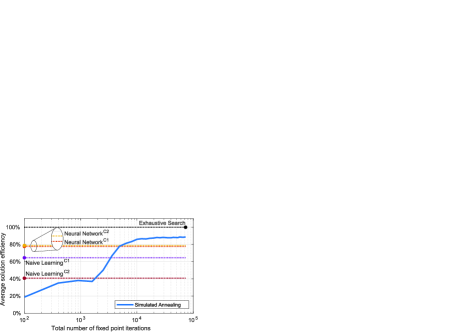
Fig. 3: Average solution efficiency as a function of the number of fixed point iterations.

5 Conclusion

In this work, we proposed a method that jointly optimizes the beam configuration, UE-AP assignments, and the power allocation in mmWave communication systems with directional transmission. We introduced a neural network that predicts the beam configuration from UE related information, and the fixed point algorithm solves the UE-AP assignment and power allocation problems given the predicted beam configuration. One of the advantages of the proposed method is that it predicts the beam configuration non-iteratively, which is an important factor in mmWave communication systems with low-latency requirements. Another advantage of the proposed method is that the fixed point algorithm guarantees the optimal power allocation and UE-AP assignments given any prediction from the neural network. Simulations showed that the proposed method can provide 80 % of the optimal rates on average with a single call of the fixed point algorithm, while the reference method based on simulated annealing requires to solve fixed point problems repeatedly to achieve the same performance.

References

- [1] Yong Niu, Yong Li, Depeng Jin, Li Su, and Athanasios V Vasilakos, “A Survey of Millimeter Wave Communications (mmWave) for 5G: Opportunities and Challenges,” Wireless networks, vol. 21, no. 8, pp. 2657–2676, 2015.
- [2] “IEEE Standard for Information Technology – Telecommunications and Information Exchange between Systems Local and Metropolitan Area Networks–Specific Requirements Part 11: Wireless LAN Medium Access Control (MAC) and Physical Layer (PHY) Specifications,” IEEE Std 802.11-2012 (Revision of IEEE Std 802.11-2007), pp. 1–2793, 2012.
- [3] M. Zeng, W. Hao, O. A. Dobre, and H. V. Poor, “Energy-Efficient Power Allocation in Uplink mmWave Massive MIMO With NOMA,” IEEE Trans. Veh. Technol., vol. 68, no. 3, pp. 3000–3004, March 2019.
- [4] Sungoh Kwon and Joerg Widmer, “Multi-beam Power Allocation for mmWave Communications under Random Blockage,” in 2018 IEEE 87th Vehicular Technology Conference (VTC Spring). IEEE, 2018, pp. 1–5.
- [5] Yan Liu, Zhiyuan Jiang, Shunqing Zhang, and Shugong Xu, “Deep Reinforcement Learning-Based Beam Tracking for Low-Latency Services in Vehicular Networks,” in ICC 2020-2020 IEEE International Conference on Communications (ICC). IEEE, 2020, pp. 1–7.
- [6] Ke Ma, Dongxuan He, Hancun Sun, Zhaocheng Wang, and Sheng Chen, “Deep Learning Assisted Calibrated Beam Training for Millimeter-Wave Communication Systems,” arXiv preprint arXiv:2101.05206, 2021.
- [7] R. Ismayilov, M. Kaneko, T. Hiraguri, and K. Nishimori, “Adaptive Beam-Frequency Allocation Algorithm with Position Uncertainty for Millimeter-Wave MIMO Systems,” in 2018 IEEE 87th Vehicular Technology Conference (VTC Spring), June 2018, pp. 1–5.
- [8] Sylvester Aboagye, Ahmed Ibrahim, and Telex MN Ngatched, “Energy Efficient User Association, Power, and Flow Control in Millimeter Wave Backhaul Heterogeneous Networks,” IEEE Open Journal of the Communications Society, vol. 1, pp. 41–59, 2019.
- [9] Shubhajeet Chatterjee, Mohammad J Abdel-Rahman, and Allen B MacKenzie, “Robust Access Point Deployment and Adaptive User Assignment for Indoor Millimeter Wave Networks,” in ICC 2020-2020 IEEE International Conference on Communications (ICC). IEEE, 2020, pp. 1–6.
- [10] R. Ismayilov, B. Holfeld, R. L. G. Cavalcante, and M. Kaneko, “Power and Beam Optimization for Uplink Millimeter-Wave Hotspot Communication Systems,” IEEE Wireless Communications and Networking Conference, pp. 1–8, April 2019.
- [11] Renato L. G. Cavalcante, Qi Liao, and Slawomir Stańczak, “Connections Between Spectral Properties of Asymptotic Mappings and Solutions to Wireless Network Problems,” IEEE Transactions on Signal Processing, vol. 67, no. 10, pp. 2747–2760, 2019.
- [12] Grigorios Tsoumakas and Ioannis Katakis, “Multi-label Classification: An Overview,” International Journal of Data Warehousing and Mining (IJDWM), vol. 3, no. 3, pp. 1–13, 2007.
- [13] Shie Mannor, Dori Peleg, and Reuven Rubinstein, “The Cross Entropy Method for Classification,” in Proceedings of the 22nd International Conference on Machine Learning, New York, NY, USA, 2005, ICML ’05, p. 561–568, Association for Computing Machinery.
- [14] 5GCM, “5G Channel Model for Bands up to 100 GHz,” Tech. Rep., Oct, 2016.
- [15] Matthew D Zeiler, “Adadelta: An Adaptive Learning Rate Method,” arXiv preprint arXiv:1212.5701, 2012.