Chi-square and normal inference in high-dimensional multi-task regression
Abstract
The paper proposes chi-square and normal inference methodologies for the unknown coefficient matrix of size in a multi-task linear model with covariates, tasks and observations under a row-sparse assumption on . The row-sparsity , dimension and number of tasks are allowed to grow with . In the high-dimensional regime , in order to leverage the row-sparsity [33, 42], the multi-task Lasso is considered.
We build upon the multi-task Lasso with a de-biasing scheme to correct for the bias induced by the penalty. The de-biasing scheme requires the introduction of a new data-driven object, coined the interaction matrix, that captures the effective correlations between noise vector and residuals on different tasks. The interaction matrix is symmetric positive semi-definite, of size and can be computed efficiently.
The interaction matrix lets us derive asymptotic normal and asymptotic results under general Gaussian design and the rate condition which corresponds to consistency in Frobenius norm of the multi-task Lasso. These asymptotic distribution results yield valid confidence intervals for single entries of and valid confidence ellipsoids for single rows of . If the covariance of the design is unknown, a modification of the multi-task de-biasing scheme using the nodewise Lasso provides comparable confidence intervals and confidence ellipsoids for the -th row of , provided that the -th column of the precision matrix is sufficiently sparse. While previous proposals in grouped-variables regression require row-sparsity up to constants depending on and logarithmic factors in for unknown , the de-biasing scheme using the interaction matrix provides confidence intervals and confidence ellipsoids under the conditions and
allowing for row-sparsity when up to logarithmic factors.
1 Introduction
1.1 Model
We consider a multi-task linear regression model with tasks, with i.i.d. observations , where is a random feature vector and are different scalar responses. We assume that on each task , the response satisfies a linear model
| (1.1) |
where is the unknown coefficient vector on the task . Throughout, is the design matrix with rows . The linear models (1.1) may be rewritten in vector and matrix form
| (1.2) |
where and are vectors in , is the response matrix with columns , is a noise matrix with columns , and is an unknown coefficient matrix with columns .
Estimation of in the above multi-task model has been well studied during the last decade in the high-dimensional regime where , see for instance [33]. This literature on multi-task learning suggests to use a joint convex optimization problem over the tasks in order to estimate , namely
where is the -th canonical basis vector, is the Frobenius norm of matrices and is a convex penalty function. The role of the convex penalty is to promote a shared structure on the coefficient vectors . The most common shared structure is that of row-sparsity where one assumes that only a few features are relevant across all tasks: there is a support set of small cardinality (relatively to ) such that for every task , . Equivalently, if and only if , i.e., only rows of are nonzero. In this case, the sparsity pattern encoded by is shared on all tasks, and previous literature on estimation in this setting uses a penalty proportional to the norm, , or alternatively its Elastic-Net version for non-negative tuning parameters . If the row-sparsity assumption holds and such penalty is used, estimation of by is improved compared to estimating separately [33].
1.2 Noise and residuals: non-trivial correlations for non-separable penalties
Classical multivariate statistics studies the least-squares estimate , which corresponds to in the above minimization problem. Here, the estimation on two tasks is independent, as on the -th task for we have for the -th canonical basis vector : the estimator of the unknown regression vector on the -th task only depends on the -th response , and is independent of the other responses . By independence, if the noise has i.i.d. mean-zero entries, then
| (1.3) |
i.e., residual and noise on two different tasks are uncorrelated. A similar story holds for multi-task Ridge regression, which corresponds to in the above minimization problem. The optimization problem is separable in the sense that
equivalently define . It follows again that only depends on the -th response , and if has i.i.d. mean-zero entries then (1.3) holds also for by independence.
The situation is more complex for non-separable penalty functions, for instance if the penalty is proportional to the norm, where is the -th canonical basis vector. The corresponding estimator studied throughout the paper is the multi-task Lasso
| (1.4) |
The estimate of the unknown vector on the -th task depends in an intricate way on all the responses including . Note that this dependence of on all responses is purposeful: we hope to leverage a shared pattern on all tasks (e.g., if is row-sparse and a sparsity pattern is shared by all ) in order to improve estimation compared to or . In this case, however, (1.3) does not hold and the correlation between the residual on task and the noise on task is non-trivial. Our results below (specifically Lemma F.1) reveal that for ,
when the noise has i.i.d. entries and is the entry of a symmetric matrix defined in Section 2. This matrix plays a central role in the present paper to derive asymptotic normality and asymptotic results.
1.3 Confidence intervals for linear functionals of
A first goal of the present paper is to provide confidence intervals for linear functionals of the regression vector on the first task. Throughout the paper, regarding asymptotic normality and confidence intervals, is a fixed direction of interest and we wish to construct confidence intervals for . For instance, the direction may be of the following form.
-
(i)
a canonical basis vector . For , the goal is to construct confidence intervals for , the coefficient of the -th feature on the first task. This is the classical goal in statistics where one wishes to provide inference on the effect of the -th covariate.
-
(ii)
a new feature vector , that may for instance correspond to the characteristics of a new subject whose responses are not known yet. The goal is to provide a confidence interval for which corresponds to the expected response of conditionally on the feature vector .
We stress here that the first task () has a special role: the unknown parameter only involves the first unknown coefficient vector and not the other coefficient vectors . If a single linear model is observed, the construction of confidence intervals for has been extensively studied. Most related to the present paper, [56, 51, 26, 27] initially provided methodologies for de-biasing (or de-sparsifying) the Lasso for construction of confidence intervals in a canonical basis direction for sparsity , [28] extended the sparsity requirement to , [58, 11, 13, 14, 59, 5] studied estimation and construction of confidence intervals in dense direction , and [6] extended the de-biasing methodologies to arbitrary convex penalties.
Of course, one could throw away the responses and use only the response with the aforementioned methodologies, since our goal is to construct confidence intervals for . However, throwing away the responses on tasks should intuitively lead to information loss and is not desirable.
1.4 Asymptotic results and confidence ellipsoids for rows of
The second goal of the paper is to develop confidence ellipsoids for whole rows of the unknown matrix . The -th row of is the vector in where is the -th canonical vector. Given a confidence level , a confidence ellipsoid for is a subset of constructed from the data such that
where converges to 0 as . Ideally, the confidence ellipsoid enjoys the exact nominal coverage probability asymptotically in the sense that
| (1.5) |
as . Note that one could also consider confidence sets that are not ellipsoids (e.g., hyperrectangles); we focus here on ellipsoids as they are the natural confidence sets stemming from -distributed pivotal quantities. As in classical multivariate statistics, an advantage of confidence ellipsoids is that they provide simultaneous confidence intervals for every direction , that is, when (1.5) holds and is closed and convex.
Such a confidence ellipsoid allows to perform hypothesis tests of
| (1.6) |
where the null hypothesis corresponds to the signal being independent of the -th feature , and is a separation radius. If a single task is observed (), it is impossible to distinguish between the null and the alternative with constant type I and type II errors unless for some constant . This follows by noting that the total variation distance between and converges to if are the same except on coordinate where with , and , for instance by Pinsker’s inequality and a standard bound on the Kullback Leibler divergence of two multivariate normals. If several tasks are observed as in the setting of interest here, we will see that it is possible to perform the hypothesis test (1.6) in situations where all nonzero coefficients of are of order , i.e., of indistinguishable order when a single task is observed.
If asymptotic normality results are available for each of the individual coefficients of (for instance such as those described in the previous subsection), a natural strategy to construct confidence ellipsoids is to sum the square of the asymptotically normal random variables and hope that the resulting sum has approximately the distribution with degrees-of-freedom. However, throughout the paper the number of tasks is allowed to grow to infinity with which results in some challenges regarding this strategy, as pointed out by [41]. For the sake of illustrating the resulting difficulty, assume that we have established the asymptotic normality of pivotal random variables by proving decompositions of the form where and the convergence in probability and hold, so that Slutsky’s theorem ensures that the pivotal quantities are asymptotically normal with . Denoting by , summing the squares of the pivotal quantities and applying the triangle inequality for the Euclidean norm on yields
| (1.7) |
While is of order , the variance and quantiles of are of constant order (specifically, holds by (F.17) below, and by [25]). This implies that a sufficient condition that ensures that and asymptotically share the same quantiles is that and . While and are sufficient to grant asymptotic normality for on the first task, the conditions and are much more stringent as they involve the number of tasks .
1.5 Asymptotics and assumptions
We will derive asymptotic normality and asymptotic results for a sequence of multi-task regression problems of increasing dimensions. For each , we consider the multi-task linear model (1.2) and and the multi-task Lasso estimate in (1.4) where , the number of tasks , dimension , tuning parameter and row-sparsity are all functions of . The dependence in is implicit and will be omitted to avoid notational burden. We will assume that the sequence of regression problems satisfies the following.
Assumption 1.1.
-
(i)
is a Gaussian design matrix with i.i.d. rows;
-
(ii)
is a row-sparse unknown matrix with at most nonzero rows;
-
(iii)
is a Gaussian noise matrix with i.i.d. entries;
-
(iv)
are positive and satisfy and , this implies ;
-
(v)
The spectrum of is bounded: for some constants which are independent of ;
-
(vi)
satisfies ;
-
(vii)
For two constants , the tuning parameter in (1.4) is given by
| (1.8) |
1.6 Related literature
For integers , the multi-task setting above bears resemblance with the single-response linear model of the form
| (1.9) |
where , , , and the features are partitioned into groups with equal sizes. Indeed, with , and by vectorizing the matrices in (1.1), our multi-task setting is in one-to-one correspondence with the single-response linear model (1.9) with , , block diagonal with blocks each equal to , and the partition of into groups is given by . With this correspondence, the estimator is the group Lasso where . Inference for grouped variables in a single-response linear model (1.9) focuses on estimation, hypothesis tests or confidence sets for the vector for a group of interest. In the single task setting (1.9) with grouped variables, [41] extends the de-biasing methodology in [56, 51] to inference for grouped variables and provides asymptotic distribution results. The paper [41] already describes some challenges of chi-square inference in high-dimension (cf. the discussion after (1.7)); the multi-task problem of the present paper shares some of these challenges, however our approach and proofs have no overlap with that of [41]. The papers [47, 52] give a different extension of the de-biasing methodology of [56, 51] to the group setting, again based on the group Lasso, but here by estimation of the inverse covariance matrix restricted to the group of interest with a multi-task estimator penalized by the nuclear norm. False Discovery Rate control in single-task linear models with grouped variables has been studied in [12] with a group SLOPE estimator. Under weak assumptions (in particular, no assumption on ), [37] provides an approach to inference for grouped variables, although the resulting confidence regions are conservative. The papers [34, 35] study group inference in a sequence rejection fashion when the groups are hierarchically ordered. Bootstrap methods based on the group Lasso are studied in [57], without trying to remove the bias. The paper [20] develops conservative inference methods for quantities of the form for a group of interest and a given positive definite matrix , based on the quadratic program de-biasing methodology given in [56, 26]. Finally, [6] introduces a degrees-of-freedom adjustment for the group Lasso to perform inference on a single coordinate or linear form of the unknown regression vector in (1.9).
Some papers focus on estimation and inference in the multi-task model (1.2). The papers [52, 8] study multi-task models of the form (1.2) where the noise has i.i.d. rows, and the entries within each row are correlated. A multi-task extension of the square-root Lasso is developed to concurrently estimate and the correlations in the noise . Such results on estimating the correlations of the entries in are useful to de-bias the group Lasso in the single-task model [52]. Support recovery through bounds on the group norm is studied in [36] under a mutual incoherence assumption on . The mutual incoherence assumption requires a row-sparsity level if has i.i.d. entries. Closest to the setup and goals of the present paper, [17] extends the de-biasing methodology of [56, 51] to the multi-task setting, using the nodewise Lasso to estimate a column of the precision matrix of the design. This approach requires row-sparsity of of order up to logarithmic factors. Although our approach also involves the nodewise Lasso to estimate columns of the precision matrix, the de-biasing methodology significantly differs from [17] and cannot be seen as a straightforward extension of [56, 51]: our approach requires the introduction of a data-driven symmetric matrix of size which captures the interactions between the residuals on different tasks. Introduction of this novel object lets us significantly relax the requirement on the row-sparsity of while obtaining normal and inference results, that are proved to be non-conservative under some assumption on .
1.7 Adjustments in high-dimensional inference
In single-task models, recent literature on high-dimensional inference has highlighted the necessity to adjust classical inference principles with scalar adjustments. To describe such adjustments consider a single-task linear model with , Gaussian noise and with i.i.d. rows, where an initial estimator is available. If one is interested in confidence intervals for the projection in some direction normalized with , a 1-step MLE correction in direction [54], i.e., maximizing the likelihood over the one-dimensional model yields the corrected estimate
| (1.10) |
where when ; and the direction is the one that maximizes the Fisher information [54]. (Since concentrates around , we allow ourselves to replace by in (1.10) in this informal discussion). In high dimensions, this general principle requires a modification that accounts for the degrees-of-freedom of : [27, 5] for the Lasso and [6] for general penalty suggest to amplify the correction with the degrees-of-freedom adjustment and to use the estimate
| (1.11) |
instead of (1.10). If is the Lasso, the adjustment is required for efficiency for large sparsity levels [5]. For the Lasso, the data-driven adjustment may be replaced by a deterministic scalar adjustment, i.e.,
| (1.12) |
where and is the scalar parameter obtained after solving the system of two equations with two unknowns in [40, Proposition 3.1]. The correspondence between and can be seen in [40, Theorem F.1] or [16, Section 3.3]. This system of two nonlinear equations first appeared in [1] for the Lasso and can be extended to permutation invariant penalty functions (see [15] and the references therein) and robust M-estimators [50].
1.8 Contributions
To summarize Sections 1.3 and 1.4, the inferential goals of the paper are twofold:
-
(i)
To construct valid confidence intervals for a linear functional of the unknown coefficient on the first task, by leveraging responses on all tasks simultaneously.
-
(ii)
To construct valid confidence ellipsoids for rows of the unknown coefficient matrix , for instance to provide hypothesis tests on the nullity of the -th row of , or equivalently testing that the signal does not depend on the -th covariate.
In order to achieve these statistical goals, we introduce a new object, the data-driven symmetric matrix . Introduction of the matrix is key to equip the estimator with the inference capabilities (i) and (ii) above, as the theory and simulations of the next sections will show. This data-driven matrix generalizes, to the multi-task setting, the effective degrees-of-freedom and other scalar adjustments in single-task linear models discussed in the previous subsection. Since is symmetric, scalar adjustments are necessary in the multi-task setting and that number of adjustments is unbounded if as a function of . The fact that a growing, unbounded number of scalar adjustments would be necessary to achieve the above inference capabilities in the multi-task setting was surprising—at least to us—, since existing works on adjustments in high-dimensional statistics so far only require a bounded number of scalar adjustments.
The paper also includes contributions related to the performance of the multi-task estimator in (1.4). We improve the logarithmic dependence in tuning parameter and the known upper bounds on and compared to [33]. We also develop tools to show that the random matrix enjoys a multi-task Restricted Eigenvalue (RE) condition from [9]. Although the single-task case follows in a straightforward manner from Gordon’s escape through a mesh theorem (e.g., [44]), the multi-task version of the RE condition for the random matrix requires different tools.
1.9 Organization
The rest of the paper is organized as follows. The next section summarizes notation. Section 2 describes a new quantity, the interaction matrix that plays a major role in our estimates and confidence intervals. Section 3.1 constructs confidence intervals for when the covariance matrix of the design is known. Section 3.2 extends these results and methodologies when is unknown. Section 4 develops confidence ellipsoids for rows of . Section 5 provides an efficient way of computing the interaction matrix. Section 6 presents numerical experiments that corroborate our theoretical findings. The proofs are deferred to appendices and some intuition behind the main technical argument is given in Appendix A.
1.10 Notation
Throughout the paper, the linear model vector and matrix notation (1.2) holds. , and are all non-decreasing functions of . In all the displays of convergence (e.g., , , , ), we implicitly mean that goes to . Convergence in distribution and in probability are denoted by and .
Estimators of the unknown are denoted by . For any real , and for any integer , e.g., . We use indices to sum or loop over (i.e., over the observations), indices to sum or loop over (i.e., over the tasks), indices to sum or loop over (i.e., the covariates). The vectors , , denote the canonical basis vector of the corresponding index; the size of such canonical vector will be made explicit if it is not clear from context. The identity matrices of sizes , , are and respectively and is the zero matrix with rows and columns.
For any , is the -norm of vector, e.g., is the Euclidean norm. For any matrix , is the Frobenius norm and the operator norm, also known as the spectral norm. If is symmetric, (resp. ) denotes the smallest (resp. largest) eigenvalue of . The Moore-Penrose pseudoinverse of matrix is denoted by . The Kronecker product between two matrices , with is
for . We will use the mixed product property of Kronecker products,
| (1.13) |
whenever the dimensions are such that the matrix products and make sense. The following trace property also holds
| (1.14) |
If denotes a Schatten norm (e.g., Frobenius or spectral norm), then for any , we have
| (1.15) |
We define the vectorization of any matrix by stacking vertically the columns of into a column vector in , i.e.,
For any three matrices such that the matrix product makes sense, the above vectorization operator satisfies
| (1.16) |
These many properties of Kronecker products are referenced in Section 4.2 of [23].
We consider restrictions of vectors (respectively matrices) by zeroing the corresponding entries (respectively columns). More precisely, if and then is the vector with if and if . If and , is a matrix of the same dimension as such that if and if , i.e., is a copy of after having zeroed the columns not indexed in . Finally, denotes the indicator function of an event , and if and if is the indicator that some index belongs to .
2 The interaction matrix of the Multi-Task Lasso estimator
We consider the multi-task Lasso estimator, with penalty, given (1.4) for some tuning parameter . Let denote the set of nonzero rows of . We will refer to as the support of and denote by its cardinality. The above estimator is the one commonly used in the multi-task learning literature under a row-sparsity assumption on , see, e.g., [33]. Recall that is a copy of obtained after zeroing the columns not belonging to . Define where denotes the Kronecker product defined in Section 1.10, so that is block-diagonal with blocks, each equal to . Consequently is also block-diagonal with blocks equal to . For any , define the matrix
| (2.1) |
and note that is proportional to an orthogonal projection of rank . The matrix is the Hessian of at . Finally, let be the matrix defined by .
Definition 1.
The interaction matrix of the estimator in (1.4) is defined entrywise by
| (2.2) |
for all , where denotes the Moore-Penrose inverse. Equivalently, if then
or with Kronecker product notation,
| (2.3) |
Observe that is a block-diagonal matrix with diagonal blocks equal to . For any square matrices, holds for a permutation matrix that only depends on the dimensions of and . This permutation is particularly simple and known as a perfect shuffle. It follows that is block diagonal with diagonal blocks for some permutation matrix . Thus the matrix
| (2.4) |
appearing in (2.2)-(2.3) is the sum of two matrices of size , each summand being block diagonal but in a different basis. If then and is diagonal as can be inverted by block. This corresponds to the unregularized least-squares estimate discussed in (1.2) with depending on the -th response only. In the case of interest here, the matrix induces nonzero entries outside of the diagonal blocks of , the matrix (2.4) is not diagonal by block and the resulting matrix is not diagonal. Additional structure in (2.4) and is studied in Section 5, which yields an efficient and practical algorithm to compute .
The interaction matrix plays a major role in the construction of our confidence intervals for as well as for chi-square inference regions for rows of . A high-level interpretation of its role is that captures the correlation between the residuals on different tasks. The following proposition summarizes some useful properties of . Result (iii) is important as our confidence interval for defined in the next section will involve the inverse of . Proposition 2.1 is proved in Appendix B of the supplement.
Proposition 2.1.
Let be defined by (2.2). Then
-
(i)
is symmetric and positive semi-definite.
-
(ii)
If is rank then the spectral norm of is bounded from above as .
-
(iii)
If is rank and then is positive-definite and
.
3 Asymptotic normality and confidence intervals in the multi-task setting
3.1 Known : Pivotal random variable, asymptotic normality and confidence intervals
We assume throughout this section that the direction of interest is normalized with . This normalization assumption is relaxed in the next Section 3.2 where we develop a methodology for unknown . If is known, our main result is the following where denotes the interaction matrix (2.2).
Theorem 3.1.
Let Assumption 1.1 be fulfilled. Assume that . If then
| (3.1) |
for any . Hence for , the parameter of interest satisfies
| (3.2) |
Theorem 3.1 is proved in Appendix E. The left-hand sides of both displays in Theorem 3.1 can be interpreted as Z-scores that have asymptotically standard normal distribution. In the second display, the only unknown quantity on the left hand side is , the parameter of interest (while in the first display, the only unknown quantity is the scalar ). Consequently if is the quantile of the standard normal distribution such that , an asymptotic confidence interval for is given by where
(3.2) in Theorem 3.1 states that as .
The confidence interval is centered at (which can be interpreted as the initial estimate of given by the estimator in (1.4)) plus a de-biasing correction that involves the interaction matrix through the matrix inverse
| (3.3) |
The fact that penalized estimators such as (1.4) require a de-biasing correction should be expected since it is already the case for for the Lasso [56, 51, 26, 27, 28, 5] and any regularized least-squares [6]. However, the apparition in the de-biasing correction of the interaction matrix through the matrix inverse (3.3) is surprising at least to us: we did not expect the multi-task de-biasing correction to require a matrix inversion such as (3.3) when initially tackling this problem. The length of the confidence interval above is when , and an estimate of this norm is given by the following theorem.
Theorem 3.2.
Let the assumptions and setting of Theorem 3.1 be fulfilled.
Then
when .
Consequently the length of the confidence interval is approximately which is the typical length for two-sided confidence intervals for an unknown mean when observing i.i.d. with . Theorems 3.1 and 3.2 are proved together in Appendix E.
Comparison with single-task Lasso on the first task.
It is instructive to compare the above confidence interval with the confidence interval induced by a single-task Lasso estimator computed on , i.e., when throwing away the responses on tasks . This is also a good opportunity to analyse the form of and the matrix inversion (3.3) in the degenerate case where a single task is observed.
For , a response vector in is observed and the estimator (1.4) reduces to the usual Lasso with response vector ,
The asymptotic normality result in Theorem 3.1 for asserts that
| (3.4) |
In the degenerate case , the matrices in (2.1) are all zeros and the matrix reduces to a scalar equal to where is the support of the Lasso . Here is the usual effective degrees-of-freedom for the Lasso. The factor in (3.4) is the degrees-of-freedom adjustment for the Lasso studied in [5], which is required for the asymptotic normality result (3.4) when [5]. So Theorem 3.1 reduces to the asymptotic normality result of [5] in the degenerate case , and in this case the matrix inversion (3.3) reduces to a degrees-of-freedom adjustment through the scalar multiplication by . The length of the resulting confidence interval for when (or when the tasks ) are thrown away) is then
| (3.5) |
We may compare the lengths of the two confidence intervals:
-
•
The confidence interval based on (3.2) using the responses on all tasks with length , and
- •
The length of the confidence interval based on and the responses on all tasks is smaller than the length (3.5) only when
| (3.6) |
Our simulations in Section 6 (see Figure 5) reveal that (3.6) holds, in some situations with significant margins, when is not too large. Since the comparison (3.6) can be performed by looking at the data, the practitioner should choose the multi-task confidence interval based on (3.2) over the single-task confidence interval based on (3.4) when (3.6) holds. When performing this comparison, two tests are constructed which calls for a Bonferroni correction to avoid invalid coverage due to multiple testing.
3.2 Unknown : Pivotal random variable, asymptotic normality and confidence intervals
The knowledge of is not available in most practical situations and the methodology of the previous subsection cannot be applied. Indeed the left hand sides in Theorem 3.1 involve which cannot be directly constructed from the data when unknown. Another issue that arises when is unknown is that one cannot verify the normalization required in Theorem 3.1. Intuitively, though, if it was possible to estimate both and fast enough, replacing these quantities by their estimates in (3.2) should not break asymptotic normality. Following ideas from the early de-biasing literature [56, 27, 51], we consider a direction
| (3.7) |
for some fixed covariate and compute the nodewise Lasso
| (3.8) |
for regressing on , where is the matrix with -th column replaced by a column of zeros, is a consistent estimate of and is a small constant. Alternatively, one may use the scale invariant version of (3.8) again for regressing on ,
| (3.9) |
known as Scaled lasso [48] or square-root Lasso [7], and (3.9) is equal to (3.8) with . We finally set
| (3.10) |
This corresponds to the residuals of the estimator in the linear model
| (3.11) |
with response vector , design matrix , true regression vector (so that and for ), and Gaussian noise vector independent of with distribution where . The relationship between and is the well known connection between precision matrix and linear regression for multivariate normal random vectors (see, e.g., [38, 49]).
The estimators in (3.8) and (3.9) both satisfy inequalities
| (3.12) | ||||
| (3.13) |
provided that . Inequality (3.13) is the usual estimation rate for the Lasso [9] or the Scaled Lasso [49, 7], and represents a high-probability lower bound on the restricted eigenvalue in the linear model (3.11) [44]. Inequality (3.12) follows from the KKT conditions of (3.8) for the Lasso, and from the KKT conditions of (3.9) combined with which holds thanks to properties of the Scaled or square root Lasso [49, 7]. Inequalities (3.12)-(3.13) are the only properties of that we will use in the proof of the following result. Other estimators could be used, for instance ones based on the Dantzig selector, as long as (3.12)-(3.13) are satisfied.
Theorem 3.3.
Consider a canonical basis direction for some and let Assumption 1.1 be fulfilled. Additionally assume that the sparsity of satisfies either
| (3.14) |
or
| (3.15) |
Then for any estimator satisfying (3.12)-(3.13) and every fixed we have
| (3.16) |
Asymptotic normality (3.16) still holds if in the denominator is replaced by either or .
Theorem 3.3 is proved in Section G.1.
4 Confidence ellipsoids for rows of
4.1 Known
We first construct confidence ellipsoids with the knowledge of .
Theorem 4.1.
Define the observable positive semi-definite matrix as well as
| (4.1) |
Then under Assumption 1.1, there exists a random variable with chi-square distribution with degrees of freedom such that
as well as
Consequently,
-
(i)
holds if additionally , and
-
(ii)
holds if additionally .
Theorem 4.1 is proved in Appendix F. The following proposition with relates the -quantile of to that of when either (i) or (ii) above holds.
Proposition 4.2.
Let be a sequence of random random variables and a sequence of random variables with chi-square distribution with degrees-of-freedom, where is function of (in particular, as is allowed). If is a fixed constant not depending on and is the quantile defined by then
-
(i)
implies that and
-
(ii)
implies that
Proposition 4.2 is proved in Appendix F. If , the order of is given by
| (4.2) |
where is the standard normal quantile defined by . A short proof of (4.2) is given around (F.17); see [41] for related discussions. However, using itself to construct confidence sets should be preferred in practice to avoid the approximation error in (4.2).
Combining the above two results provides confidence ellipsoids for the rows of , or more generally for the unknown vector for a fixed direction of interest. Let be the subset of defined by
Since where this set is an ellipsoidal region with center . If
| (4.3) |
additionally to Assumption 1.1 as required in case (i) of Theorem 4.1, then . If additionally
| (4.4) |
as required in case (ii) for the lower bound, then and the above confidence ellipsoid provides the exact nominal coverage (i.e., it is provably non-conservative). Note that the upper bound (i) is more important than the lower bound (ii) since the upper bound (i) guarantees that the type I error in the hypothesis test (1.6) is at most , i.e., . It is thus fortuitous that only the weak additional condition (4.3) is required for the upper bound (i) to guarantee the desired type I error, while the more stringent condition (4.4) is only required to prove non-conservativeness.
The additional assumption (4.3) is satisfied for a large class of growths of . For instance it holds under polynomial growth or exponential growth of the form for constants , as is then satisfied. Although we believe that the mild condition (4.3) is an artefact of the proof, it is unclear at this point how to relax (4.3) unless a different ellipsoid is considered. In Section 4.3, we will construct a different ellipsoid that does not require the extra conditions (4.3) or (4.4) but that has worse performance in simulations.
The radius of i.e., the half-length of its largest axis is given by
| (4.5) |
Since by Proposition 2.1 and Lemma C.3 on the one hand, and all eigenvalues of are of order by the arguments in the proof of Lemma F.3 on the other hand, the radius (4.5) is which is of order by (4.2).
The random vector (4.1) involves multiplication by which differs from the pivotal quantity in the asymptotic normality result (3.1). However, Theorem 4.1 still holds with in (4.1) replaced by
| (4.6) |
Indeed, with
Since the eigenvalues of are all of order , since by Proposition 2.1 and since by Theorem F.2, the previous display is and converges to 0 in probability by Assumption 1.1. Under Assumption 1.1, Theorem 4.1 thus holds for in (4.1) if and only if it holds for . Furthermore the corresponding ellipsoid,
enjoys the same properties as : Type I error guarantees under (4.3), and non-conservativeness under (4.4).
4.2 Unknown
A similar result is available if is unknown. Consider the notation (3.10) from Section 3.2.
Theorem 4.3.
Consider a canonical basis direction for some and let Assumption 1.1 be fulfilled. Additionally assume that either (3.14) or (3.15) holds. Then for any estimator satisfying (3.12)-(3.13),
| (4.7) |
where is a random variable with chi-square distribution with degrees-of-freedom.
Theorem 4.3 is proved in Section G.2. The corresponding confidence ellipsoid for the -th row of is
If either one of the condition (3.14) or (3.15) holds on the growth of the sparsity of , this confidence ellipsoid does not require the knowledge of and has the same guarantees as those of the previous section.
4.3 Relaxing the additional assumptions (4.3) and (4.4)
Instead of normalizing using as in the previous sections, a simple estimate of lets us relax the conditions (4.3) and (4.4) that are required in the previous section to ensure .
Theorem 4.4.
Let be defined in (4.1) and (4.6) respectively, and let . Then under Assumption 1.1, there exists a random variable with chi-square distribution with degrees of freedom such that
| (4.8) |
Theorem 4.5.
Consider a canonical basis direction for some and let Assumption 1.1 be fulfilled. Additionally assume that either (3.14) or (3.15) holds. Then for any estimator satisfying (3.12)-(3.13),
| (4.9) |
where is a random variable with chi-square distribution with degrees-of-freedom.
The above asymptotic chi-square results hold under the same assumptions as Theorem 3.1 and Theorem 3.3. The reason for the success of these estimates is that estimates at a rate faster than : we have by Theorem F.2. However, simulations in Section 6 reveal that the asymptotic estimates of the previous subsections involving the matrix are more robust to larger sparsity levels, although Assumption 1.1 is oblivious to this phenomenon.
The corresponding confidence ellipsoid for based on (4.8) and is
| (4.10) |
and satisfies under Assumption 1.1. Similar confidence ellipsoids based on (4.9) can be readily constructed.
4.4 Hypothesis testing
We now turn to type II error for the testing problem
| (4.11) |
where is a separation radius. The hypothesis test (4.11) at level is naturally achieved by rejecting if and only if for the ellipsoid in (4.10). Similar rejection procedures can be obtained with or for the confidence ellipsoids defined in Sections 4.1 and 4.2.
We can also determine the separation radius required so that this testing procedure has nontrivial power (type II error). Focusing here on in (4.10), rejection happens if and only if the following quantity is positive
where and by (4.8). By Theorem 3.1 applied to , the last line is of the form so that it is of order . The second line is positive, of order ; this is the quantity that should dominate in order to ensure that the above display is positive. Since the first line is positive with probability at least by Proposition 4.2, we obtain that if for , then the type II error is at most . Although this type II error is typically a constant close to 1 (e.g. if , this shows that the above test has at most constant type II error as long as the separation radius satisfies . We can also find conditions on that ensures that the type II error is smaller than any constant. The first line above is of order since and by Proposition 4.2 and (4.2). Thus is sufficient in order for to dominate both the first and third lines with probability approaching one. In summary, is sufficient to achieve a constant type II error, while is sufficient to grant a vanishing type II error.
In single task models, coefficients of order cannot be detected, cf. the discussion after (1.6). Here on the other hand in the multi-task setting with , detection of non-zero vector is possible with constant power even if the individual coefficients in are for any slowly increasing with . If , the coefficients are individually impossible to detect, while detection of the row vector is possible with constant type I and type II errors. Similarly, if the individual coefficients are of order for any slowly increasing with , the above testing procedure for the row vector has vanishing type II error.
5 Computing the interaction matrix efficiently
Equation 2.2 which defines is convenient for theoretical purposes, as the pseudoinverse suppresses invertibility issues and the form (2.2) naturally arises in the proofs, see for instance Lemmas C.7, C.8 and C.9. However, (2.2) is not computationally tractable as it involves computing a pseudoinverse of size . The goal of this section is to provide a computationally tractable representation for ; in particular we will see that one only needs to compute inverses of matrices of size . A first step when implementing is to remove all covariates such that , as dropping those indices and the corresponding columns of does not change the value of in (2.2). For the purpose of this section and only in this section, we assume without loss of generality that and that all variables are such that . However, we will keep the notation and use summation sign to emphasize that the indices and corresponding columns of have been dropped.
Before stating a formal proposition with a computationally friendly representation of the matrix , we explain the crux of the argument, which relies on the Sherman-Morrison-Woodbury inversion formula. Recall that and that for every
| (2.1) |
as well as . By splitting the part of proportional to the identity and the rank one part, we find
where is the vector with and is the square diagonal matrix with as its diagonal. By the mixed product property (1.13) we have
so that, with we obtain
where has columns and If is invertible and its inverse can be computed efficiently, the inverse of the above display is given by the Sherman-Morrison-Woodbury formula [24]: if the matrix is invertible then is also invertible and
Since has positive entries, is always invertible and so is , with
| (5.1) |
Hence we only need to perform two inversions of matrices of size : the inversion of and of .
Proposition 5.1.
With the above notation for and for each , if the matrix defined entrywise by
is invertible then
where
Proof.
By definition of and using the above Sherman-Morrison-Woodbury identity
By (1.14), the first term equals which gives the first term in the proposition, proportional to . Using again the structure of in (5.1), the second summand in the previous display is equal to
| (5.2) |
where and are given in the proposition, after noting that the definition of is equivalent to . Since has columns , the entry of the matrix is equal to
Since for two symmetric matrices of the same size, we obtain
On the last line, the matrix in bracket is the second matrix in the expression of . ∎
We now turn to implementation details. We recommend
an approach that makes use of optimized
vectorized code as often as possible
to compute the quantities in Proposition 5.1,
and if available to use a library with Einstein summation routine
as this allows the code to mimick the mathematical notation
in Proposition 5.1.
For concreteness, the following code lets us efficiently compute
with the Python library Numpy [22],
and the Einstein summation function
numpy.einsum which comes in handy.
Assume that
has been computed, the rows in removed
and the result stored in an array
B_S of size ,
that with the columns in removed
is stored in an array X_S of size ,
and that the scalar is stored in variable nTlambda.
Then the vector
and matrix with columns in variable
can be computed as follows:
Finally, matrices and
are computed using built-in symmetric matrix inversion,
while computation of and again resorts to using np.einsum:
In einsum, we use indices t and u to loop over ,
and indices j and k to loop over .
All calls to einsum can be further optimized
by pre-computing the optimal order in which tensor contractions
should be performed (see numpy.einsum_path).
Empirically, we have observed that this implementation using the Sherman-Morrison-Woodbury identity and the above code is several orders of magnitude faster than a naive one involving sparse matrices and the full inversion of .
6 Numerical experiments
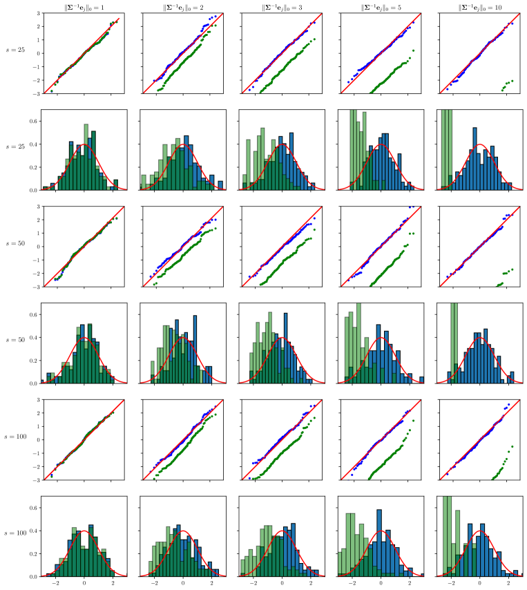
We run simulations to illustrate the theorems proved in Sections 3 and 4. The values of the parameters are fixed to , , , , . The tuning parameter is (we explain below how is constructed). The directions of interest are and .
Quantile-quantile plots of the pivotal quantities
The goal is to assess how the sparsity of and influence the convergence in Theorems 3.1, 3.3, 4.1, 4.3 and 4.5. Denote by and the respective sparsity parameters that will vary in the experiments. Given a target tuple we generate with exactly non-zero rows and with exactly non-zero entries on the first column of , so that .
We explain first how is constructed so that it satisfies the constraints in Assumption 1.1 as well as the sparsity requirement on . Start by sampling , a matrix with i.i.d. entries. Then perform the QR decomposition of to obtain an orthogonal matrix , the distribution of which is uniform in the sense of Haar measure on the orthogonal group . Next, consider , the diagonal matrix with entries and set . Define the block matrix
where is a vector with sparsity and norm . This ensures boundedness of the spectrum as the smallest eigenvalue of satisfies the lower bound
where the last equality follows from and . Similarly, the largest eigenvalue of can be bounded above by Finally set where is the greatest diagonal entry of so that . This construction leads to and .
The row-sparse matrix is constructed as follows. Initialize as a matrix filled with ’s and alter it in two different ways:
-
(i)
Setting with overlapping supports. In the first setting, we zero out rows of while forcing an overlap of the supports of and (either or the reverse inclusion). The intuition is that this makes inequality (G.1) tight. This constraint is therefore expected to slow down convergence.
-
(ii)
No-overlap setting. In the second setting this constraint is removed and the support of is picked uniformly at random as a subset of .
Assume that the tuple is fixed.
We sample instances of .
For each sample, we compute the estimator using the function MultiTaskElasticNet from the Python library Scikit-learn [43],
build the interaction matrix using the implementation from Section 5
and collect the pivotal quantities appearing in the Theorems.
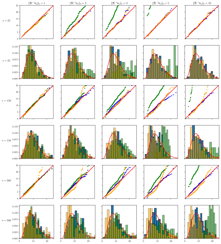
The Q-Q plots and histograms for different pairs are then reported
in Figures 1 and 2 for the overlapping supports setting
(i)
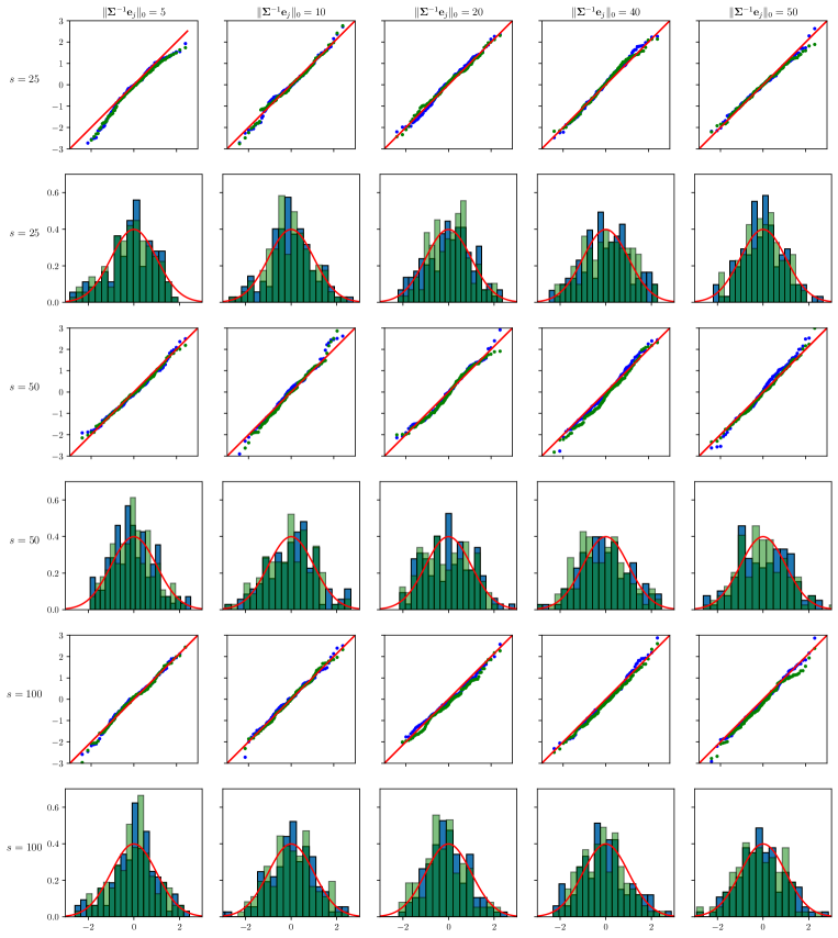
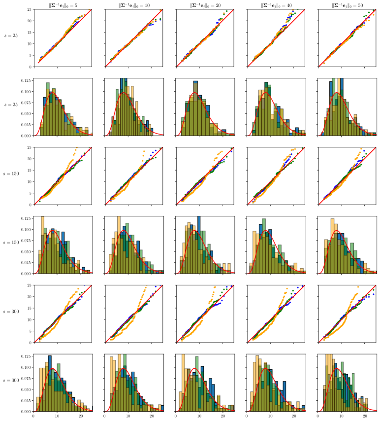
and Figures 3 and 4 for the no-overlap setting
(ii).
Asymptotic normality is observed empirically on Figure 3 in the no-overlap setting, both when is known (blue) and unknown (green). The convergence holds up well across a wide range of sparsity levels. In the overlapping supports setting of Figure 1, convergence is maintained if is known, but in the unknown case it deteriorates fast when grows. This suggests that condition (3.14) is not an artefact of the proof.
The picture is different with chi-square results. In the no-overlap setting of Figure 4, convergence is observed across all sparsity levels for pivotal quantities in Theorem 4.1 (known ) and Theorem 4.3 (unknown ) whereas an increase in slows down convergence in Theorem 4.5 (unknown ). In the overlapping supports setting (i) of Figure 2, pivotal quantities in Theorems 4.1 and 4.5 exhibit the same behavior as in the previous setting whereas the one from Theorem 4.3 shows increasingly slower convergence as grows. Again, this suggests that condition (3.14) is not an artefact of the proof.
6.1 The advantage of multi-task learning for narrower confidence intervals
In Figure 5 we illustrate the discussion around (3.6) by comparing the lengths of confidence intervals obtained via multi-task Lasso and single-task Lasso. is set to and the pair varies. For a given and a sampled we compute the relative change . We collect these values over samples and obtain the bottom figure. Since the results with or without the overlap constraint in the supports are similar, only the no-overlap setting (ii) is shown. In the upper figure, multi-task confidence interval lengths are pooled together over the samples and we compare them to the aggregate single-task lengths. As a sanity check we observe that multi-task and single-task Lasso coincide when is equal to . For , -based confidence intervals always have smaller length, which shrinks as increases. When we observe a average gain in the width. Exploiting several tasks thus provides better estimates than intervals based on the first task. However, as grows, this effect fades gradually and when it is counterbalanced by high variance in the multi-task lengths.
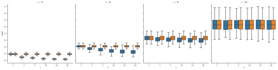
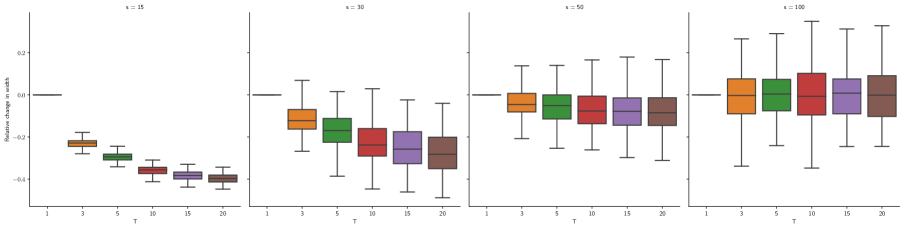
Bottom: boxplots for relative change in length with single-task as reference. Only the no-overlap setting (ii) is shown and is set to .
References
- [1] Mohsen Bayati and Andrea Montanari. The lasso risk for gaussian matrices. IEEE Transactions on Information Theory, 58(4):1997–2017, 2012.
- [2] Pierre C Bellec. Optimal bounds for aggregation of affine estimators. The Annals of Statistics, 46(1):30–59, 2018.
- [3] Pierre C Bellec and Alexandre B Tsybakov. Bounds on the prediction error of penalized least squares estimators with convex penalty. In Vladimir Panov, editor, Modern Problems of Stochastic Analysis and Statistics, Selected Contributions In Honor of Valentin Konakov. Springer, 2017.
- [4] Pierre C Bellec and Cun-Hui Zhang. Second order stein: Sure for sure and other applications in high-dimensional inference. arXiv:1804.01230, 2018.
- [5] Pierre C Bellec and Cun-Hui Zhang. De-biasing the lasso with degrees-of-freedom adjustment. arXiv preprint arXiv:1902.08885, 2019.
- [6] Pierre C Bellec and Cun-Hui Zhang. Second order poincar’e inequalities and de-biasing arbitrary convex regularizers when . arXiv preprint arXiv:1912.11943, 2019.
- [7] Alexandre Belloni, Victor Chernozhukov, and Lie Wang. Square-root lasso: pivotal recovery of sparse signals via conic programming. Biometrika, 98(4):791–806, 2011.
- [8] Quentin Bertrand, Mathurin Massias, Alexandre Gramfort, and Joseph Salmon. Handling correlated and repeated measurements with the smoothed multivariate square-root lasso. In Advances in Neural Information Processing Systems, pages 3961–3972, 2019.
- [9] Peter J. Bickel, Ya’acov Ritov, and Alexandre B. Tsybakov. Simultaneous analysis of lasso and dantzig selector. Ann. Statist., 37(4):1705–1732, 08 2009.
- [10] Stéphane Boucheron, Gábor Lugosi, and Pascal Massart. Concentration inequalities: A nonasymptotic theory of independence. Oxford University Press, 2013.
- [11] Jelena Bradic, Jianqing Fan, and Yinchu Zhu. Testability of high-dimensional linear models with non-sparse structures. arXiv preprint arXiv:1802.09117, 2018.
- [12] Damian Brzyski, Alexej Gossmann, Weijie Su, and Małgorzata Bogdan. Group slope–adaptive selection of groups of predictors. Journal of the American Statistical Association, 114(525):419–433, 2019.
- [13] T Tony Cai and Zijian Guo. Confidence intervals for high-dimensional linear regression: Minimax rates and adaptivity. The Annals of statistics, 45(2):615–646, 2017.
- [14] Tianxi Cai, Tony Cai, and Zijian Guo. Individualized treatment selection: An optimal hypothesis testing approach in high-dimensional models. arXiv preprint arXiv:1904.12891, 2019.
- [15] Michael Celentano and Andrea Montanari. Fundamental barriers to high-dimensional regression with convex penalties. arXiv preprint arXiv:1903.10603, 2019.
- [16] Michael Celentano, Andrea Montanari, and Yuting Wei. The lasso with general gaussian designs with applications to hypothesis testing. arXiv preprint arXiv:2007.13716, 2020.
- [17] Jérôme-Alexis Chevalier, Alexandre Gramfort, Joseph Salmon, and Bertrand Thirion. Statistical control for spatio-temporal MEG/EEG source imaging with desparsified multi-task Lasso. In Thirty-fourth Conference on Neural Information Processing Systems, 2020.
- [18] Kenneth R Davidson and Stanislaw J Szarek. Local operator theory, random matrices and banach spaces. Handbook of the geometry of Banach spaces, 1(317-366):131, 2001.
- [19] Christophe Giraud, Sylvie Huet, and Nicolas Verzelen. High-dimensional regression with unknown variance. Statistical Science, 27(4):500–518, 11 2012.
- [20] Zijian Guo, Claude Renaux, Peter Bühlmann, and T Tony Cai. Group inference in high dimensions with applications to hierarchical testing. arXiv preprint arXiv:1909.01503, 2019.
- [21] Wolfgang Karl Härdle and Léopold Simar. Applied Multivariate Statistical Analysis. Springer International Publishing, Cham, 2019.
- [22] Charles R. Harris, K. Jarrod Millman, Stéfan J. van der Walt, Ralf Gommers, Pauli Virtanen, David Cournapeau, Eric Wieser, Julian Taylor, Sebastian Berg, Nathaniel J. Smith, Robert Kern, Matti Picus, Stephan Hoyer, Marten H. van Kerkwijk, Matthew Brett, Allan Haldane, Jaime Fernández del Río, Mark Wiebe, Pearu Peterson, Pierre Gérard-Marchant, Kevin Sheppard, Tyler Reddy, Warren Weckesser, Hameer Abbasi, Christoph Gohlke, and Travis E. Oliphant. Array programming with NumPy. Nature, 585(7825):357–362, September 2020.
- [23] Roger A. Horn and Charles R. Johnson. Topics in matrix analysis. Cambridge University Press, Cambridge, 1991.
- [24] Roger A. Horn and Charles R. Johnson. Matrix Analysis. Cambridge University Press, 2 edition, 2012.
- [25] J.G. (https://math.stackexchange.com/users/56861/j g). Limiting value of the variance of the distribution (square root of distribution). Mathematics Stack Exchange. URL:https://math.stackexchange.com/q/3376610 (version: 2019-10-01).
- [26] Adel Javanmard and Andrea Montanari. Confidence intervals and hypothesis testing for high-dimensional regression. The Journal of Machine Learning Research, 15(1):2869–2909, 2014.
- [27] Adel Javanmard and Andrea Montanari. Hypothesis testing in high-dimensional regression under the gaussian random design model: Asymptotic theory. IEEE Transactions on Information Theory, 60(10):6522–6554, 2014.
- [28] Adel Javanmard and Andrea Montanari. Debiasing the lasso: Optimal sample size for gaussian designs. The Annals of Statistics, 46(6A):2593–2622, 2018.
- [29] jlewk (https://math.stackexchange.com/users/484640/jlewk). Is it true that implies for singular positive semi-definite matrices? Mathematics Stack Exchange. URL:https://math.stackexchange.com/q/3682798 (version: 2020-05-20).
- [30] jlewk (https://math.stackexchange.com/users/484640/jlewk). Lipschitz continuity of . Mathematics Stack Exchange. URL:https://math.stackexchange.com/q/3968118 (version: 2020-12-31).
- [31] B. Laurent and P. Massart. Adaptive estimation of a quadratic functional by model selection. Ann. Statist., 28(5):1302–1338, 10 2000.
- [32] Christopher Liaw, Abbas Mehrabian, Yaniv Plan, and Roman Vershynin. A simple tool for bounding the deviation of random matrices on geometric sets. In Geometric aspects of functional analysis, pages 277–299. Springer, 2017.
- [33] Karim Lounici, Massimiliano Pontil, Sara Van De Geer, and Alexandre B Tsybakov. Oracle inequalities and optimal inference under group sparsity. The annals of statistics, 39(4):2164–2204, 2011.
- [34] Jacopo Mandozzi and Peter Bühlmann. Hierarchical testing in the high-dimensional setting with correlated variables. Journal of the American Statistical Association, 111(513):331–343, 2016.
- [35] Jacopo Mandozzi and Peter Bühlmann. A sequential rejection testing method for high-dimensional regression with correlated variables. The international journal of biostatistics, 12(1):79–95, 2016.
- [36] Mathurin Massias, Quentin Bertrand, Alexandre Gramfort, and Joseph Salmon. Support recovery and sup-norm convergence rates for sparse pivotal estimation. arXiv preprint arXiv:2001.05401, 2020.
- [37] Nicolai Meinshausen. Group bound: confidence intervals for groups of variables in sparse high dimensional regression without assumptions on the design. Journal of the Royal Statistical Society: Series B (Statistical Methodology), 77(5):923–945, 2015.
- [38] Nicolai Meinshausen and Peter Bühlmann. High-dimensional graphs and variable selection with the lasso. The annals of statistics, 34(3):1436–1462, 2006.
- [39] metamorphy (https://math.stackexchange.com/users/543769/metamorphy). Inequality involving the gamma function: . Mathematics Stack Exchange. URL:https://math.stackexchange.com/q/3590470 (version: 2020-03-22).
- [40] Léo Miolane and Andrea Montanari. The distribution of the lasso: Uniform control over sparse balls and adaptive parameter tuning. arXiv preprint arXiv:1811.01212, 2018.
- [41] Ritwik Mitra and Cun-Hui Zhang. The benefit of group sparsity in group inference with de-biased scaled group lasso. Electronic Journal of Statistics, 10(2):1829–1873, 2016.
- [42] Guillaume Obozinski, Martin J Wainwright, and Michael I Jordan. Support union recovery in high-dimensional multivariate regression. The Annals of Statistics, 39(1):1–47, 2011.
- [43] F. Pedregosa, G. Varoquaux, A. Gramfort, V. Michel, B. Thirion, O. Grisel, M. Blondel, P. Prettenhofer, R. Weiss, V. Dubourg, J. Vanderplas, A. Passos, D. Cournapeau, M. Brucher, M. Perrot, and E. Duchesnay. Scikit-learn: Machine learning in Python. Journal of Machine Learning Research, 12:2825–2830, 2011.
- [44] Garvesh Raskutti, Martin J Wainwright, and Bin Yu. Restricted eigenvalue properties for correlated gaussian designs. The Journal of Machine Learning Research, 11:2241–2259, 2010.
- [45] Charles Stein. A bound for the error in the normal approximation to the distribution of a sum of dependent random variables. In Proceedings of the Sixth Berkeley Symposium on Mathematical Statistics and Probability, Volume 2: Probability Theory. The Regents of the University of California, 1972.
- [46] Charles M Stein. Estimation of the mean of a multivariate normal distribution. The annals of Statistics, pages 1135–1151, 1981.
- [47] Benjamin Stucky and Sara van de Geer. Asymptotic confidence regions for high-dimensional structured sparsity. IEEE Transactions on Signal Processing, 66(8):2178–2190, 2018.
- [48] Tingni Sun and Cun-Hui Zhang. Scaled sparse linear regression. Biometrika, 99(4):879–898, 2012.
- [49] Tingni Sun and Cun-Hui Zhang. Sparse matrix inversion with scaled lasso. The Journal of Machine Learning Research, 14(1):3385–3418, 2013.
- [50] Christos Thrampoulidis, Ehsan Abbasi, and Babak Hassibi. Precise error analysis of regularized -estimators in high dimensions. IEEE Transactions on Information Theory, 64(8):5592–5628, 2018.
- [51] Sara Van de Geer, Peter Bühlmann, Ya’acov Ritov, and Ruben Dezeure. On asymptotically optimal confidence regions and tests for high-dimensional models. The Annals of Statistics, 42(3):1166–1202, 2014.
- [52] Sara van de Geer and Benjamin Stucky. 2-confidence sets in high-dimensional regression. In Statistical analysis for high-dimensional data, pages 279–306. Springer, 2016.
- [53] Roman Vershynin. High-dimensional probability: An introduction with applications in data science, volume 47. Cambridge university press, 2018.
- [54] Cun-Hui Zhang. Statistical inference for high-dimensional data. Mathematisches Forschungsinstitut Oberwolfach: Very High Dimensional Semiparametric Models, Report, (48):28–31, 2011.
- [55] Cun-Hui Zhang and Jian Huang. The sparsity and bias of the lasso selection in high-dimensional linear regression. Ann. Statist., 36(4):1567–1594, 08 2008.
- [56] Cun-Hui Zhang and Stephanie S Zhang. Confidence intervals for low dimensional parameters in high dimensional linear models. Journal of the Royal Statistical Society: Series B (Statistical Methodology), 76(1):217–242, 2014.
- [57] Qing Zhou and Seunghyun Min. Uncertainty quantification under group sparsity. Biometrika, 104(3):613–632, 2017.
- [58] Yinchu Zhu and Jelena Bradic. Linear hypothesis testing in dense high-dimensional linear models. Journal of the American Statistical Association, 113(524):1583–1600, 2018.
- [59] Yinchu Zhu and Jelena Bradic. Significance testing in non-sparse high-dimensional linear models. Electronic Journal of Statistics, 12(2):3312–3364, 2018.
SUPPLEMENT
Appendix A Intuition
Let us give some rationale behind the pivotal quantities stated in the main theorems. In this paragraph and only in this paragraph for the sake of providing some intuition, we assume that for some canonical basis vector in and that so that entries of are i.i.d. . In this setting, the random vector has i.i.d. entries and is independent of , the matrix with -th column removed. Since , Stein’s formula [45, 46] states that for any differentiable vector field with , under integrability conditions. For the sake of the current informal argument, assume that Stein’s formula provides reasonable approximation. Then applying Stein’s formula to for each task (here, is the -th canonical basis vector in ), by nontrivial computations that are made rigorous in the proofs given in the supplement, the approximations
| (A.1) | ||||
hold up to smaller order terms, where is the interaction matrix in Equation 2.2. By viewing (A.1) as a linear system with equations and the unknowns , and assuming that solving the linear system maintains the approximations, we obtain that
or equivalently . Thus the matrix product of times the residuals projected onto provides us with estimates of the bias of on the direction . This informal argument is the crux of the rigorous methodology developed in the next subsections. In the sequel, we drop the assumption that . When is known as in Section 3.1, the score vector in (A.1) has to be replaced by a random vector proportional to . When is unknown as in Section 3.2, the score vector has to be estimated.
Appendix B Proof of Proposition 2.1
We restate the proposition for convenience.
See 2.1
Proof.
(i) We have the following equalities:
where follows from (2.3), is a consequence of and the mixed product property (1.13), and follow from , holds because the pseudoinverse preserves symmetry.
This proves that is symmetric. Since the pseudoinverse of a positive semi-definite matrix is positive semi-definite as well, we also have
| (B.1) |
so that is positive semi-definite.
(ii)
Recall that .
By properties of Gram matrices, , hence by the rank-nullity theorem, has dimension .
By definition of , each vector is in the kernel of for and , hence in . These vectors are linearly independent, so they form a basis of .
Besides, since , the mixed product property of Kronecker products (1.13) implies that for and , hence . Since these matrices are positive semi-definite, it is easy to check that the reverse inclusion holds as well, so that .
Since is positive semi-definite, holds in the sense of the positive semi-definite order, and
| (B.2) |
holds because the two matrices have the same kernel, see [29]. Next, using (B.1),
where the first inequality follows from (B.2) and the third and fourth line follow respectively from and the mixed product property (1.13). The last line stems from the fact that is a projection matrix of rank when .
(iii) Since has rank , we have by (ii) that . Since is positive-semi definite, its spectral norm is its largest eigenvalue, hence all the eigenvalues of are , and is positive definite. For any with we have . By the triangle inequality and the submultiplicativity of the operator norm,
∎
Appendix C Preliminaries
In this section we develop a series of technical lemmas that will be used for proving Sections 3 and 4. We consider model (1.2) and the estimator from (1.4). Let , , and set as in (1.8). Define the sparsity level
| (C.1) |
and note that is of the same order as when the spectrum of is bounded away from 0 and infinity as in Assumption 1.1. Let , and define the events
as well as
| (C.2) |
Since the only randomness is with respect to , we view the underlying probability space as and as subsets of so that occurs if and only if for each .
Lemma C.1.
Let Assumption 1.1 be fulfilled. Then .
Lemma C.2.
Lemma C.3.
On , inequality holds with in (C.1).
Lemma C.4.
On we have .
Lemma C.5.
For almost every , the KKT conditions of in (1.4) hold strictly in the sense that .
Lemma C.6.
Lemma C.7.
For almost every in the open set , is a Fréchet differentiable function of . For almost every in , if
is the estimate (1.4) with replaced by the perturbed design , then for any
as , where is a linear map given by with
for all and . Note that and implicitly depend on . Hence the matrix of size is the Jacobian of the map at .
Lemma C.8.
For any we have on
| (C.3) | ||||
| (C.4) |
for some constant depending on and only.
Lemma C.9.
Under Assumption 1.1, as we have
Since has probability approaching one, this implies that converges to 0 in probability.
We now prove each lemma. The lemmas are restated before their proofs for convenience.
See C.1
Proof of Lemma C.1.
The fact that has probability approaching one under Assumption 1.1 follows from the propositions in Appendix D: Proposition D.1 (iii) with and , Proposition D.2, Proposition D.3 applied with , and by [18, Theorem II.13]. ∎
See C.2
Proof of Lemma C.2.
In the whole proof we place ourselves on the event . We prove first that .
By the definition of ,
.
Rewriting the LHS as and expanding the square yields
.
The following chain of inequalities holds
and follow from Cauchy-Schwarz inequality, stems from the inequality and holds on . Thus
| (C.5) |
Besides, the quantity inside the bracket on the right hand side satisfies
where follows from Cauchy-Schwarz and the reverse triangle inequality applied respectively on the first and third summands of , whereas is a consequence of Cauchy-Schwarz. Combining this bound with (C.5) and plugging in the value yields
| (C.6) |
Non-negativity of the LHS, the equality
and Cauchy-Schwarz lead to
.
Since and , we get , that is .
The inequality
| (C.7) |
combined with (C.6) and the event yields
Reusing , we obtain
.
Combining this last bound with (C.7) yields
, hence (iv).
For inequality (v), using , and we have
Regarding the limit of , note that . By Assumption 1.1, each summand goes to as goes to . ∎
See C.3
Proof of Lemma C.3.
The KKT conditions of (1.4) are given by
| (C.8) |
This implies that Since by the triangle inequality, we have for any ,
| (C.9) | ||||
| (C.10) |
Summing the squares of the above inequalities for a subset and using , we get
The first term is bounded from above by on the event . Dividing by we find
where is the largest eigenvalue of , or equivalently the largest eigenvalue of , which is also the largest eigenvalue of . On the event of , we obtain
or equivalently
Let be as in (C.1) and assume that is violated on . Then on , any with size satisfies , . Squaring yields . Then
which shows that by definition of , a contradiction. ∎
See C.4
Proof.
By Lemma C.3, we have on . Since , the event yields , . If is such that and , then we must have . Equivalently, the linear span of has intersection with , hence must be contained in the span of . Thus and by the rank-nullity theorem, . By definition of , it is also clear that , hence the conclusion. ∎
See C.5
Proof of Lemma C.5.
This follows from the argument in Lemma 6.4 of [5, arXiv version v1, 24 Feb 2019]. ∎
See C.6
Proof of Lemma C.6.
By Lemma C.3, has at most non-zero rows. applied on each column of gives . Similarly, using with and summing the resulting inequality with the previous one yields
Define , and . When expanding the squares, it is clear that is the sum of a linear function and of the convex penalty, thus is convex. Additivity of subdifferentials yields . By optimality of we have , thus . This implies . Letting and , the last inequality rewrites as
Summing the similar inequality obtained by replacing with yields
Combining the above displays, we obtain
The second summand rewrites as By Cauchy-Schwarz and the submultiplicativity of the Frobenius norm, the second summand is bounded above by
Since and have respectively at most and non-zero rows, using twice gives the following bound on the second summand:
Combining the above displays, we find
Thanks to Lemma C.2 we have and , this shows that , hence
We also have by the triangle inequality
where the last line follows from the inequality for . ∎
See C.7
Proof of Lemma C.7.
By Lemma C.6 and Rademacher’s theorem, we know that the Fréchet derivative of with respect to exists almost everywhere, so that exists for almost every . By Lemma C.5, we also have that for almost every , the KKT conditions are strict in the sense given in Lemma C.5. In the following, we consider such that exists and such that the KKT conditions are strict; almost every satisfy these two conditions.
Since we know that the Jacobian exists by Rademacher’s theorem, it is enough to characterize its value, for instance by computing the directional derivative in any fixed direction . To this end, for a real in a neighborhood of , let and . Define the active set . We also write , and . At , we have and is the estimator computed at with .
As in (C.8), the KKT conditions for read, for (i.e., ),
and for (i.e., ),
By Lipschitz continuity of established in Lemma C.6, the set is constant in a neighborhood of 0 because the KKT conditions on are bounded away from on a neighborhood of 0 by continuity, and because the nonzero rows of are bounded away from in a neighborhood of again by continuity of . Differentiation of the above display for at and the product rule yield
with in (2.1). Rearranging and using ,
Let . Multiplying by to the left and summing over , we obtain
Since is locally constant for in a neighborhood of 0, we have thus , hence
We now use the relationship between vectorization and Kronecker product (1.16). Applying (1.14) to the previous display for each term, we find
Since is always a column vector, . Finally, we have again using (1.16) and the chain rule, for any fixed ,
By Lemma C.4, . The argument developed in the proof of Proposition 2.1 (ii) shows that the nullspace of the matrix is exactly the linear span of . Because , is in . Since for any symmetric matrix , is the orthogonal projection on the range of , we have Since is a column vector, using (1.16) again,
Since this holds for all , this provides the desired expression for for all . ∎
See C.8
Proof of Lemma C.8.
For (C.4), the following bounds will be useful. Inequality holds on . Furthermore since for all symmetric matrices and since is positive semi-definite, on we find
| (C.11) |
We now work on , the left hand side of (C.4). For brevity, define Then if and denote canonical basis vectors, where has components so that
where the last equality stems from two applications of the mixed product property (1.13):
Thus and since , it follows that by (1.13).
By the definition of , using the commutation property of the trace we have
By the Cauchy-Schwarz inequality for and using twice, we find
and the second factor equals by (1.15) for the Frobenius norm.
We introduce the notation to denote an inequality up to a constant that depends on and only. On we have the operator norm bound (C.11), the bound as well as so that
and thanks to and Lemma C.2. Since and under Assumption 1.1, we have proved that holds on which is exactly the desired bound (C.4).
∎
See C.9
Proof of Lemma C.9.
Recall that we assume the normalization . Following the notation in [5] we define the quantities:
We have the decomposition , the vector is independent of and has distribution . Given a value of , define the open set
Since is open , so is the set . Given a value of we also define the function given by
as well as
Since under Assumption 1.1 and is bounded by an absolute constant on when , Lemma C.6 shows that is -Lipschitz for some constant of the form where the constant depends only on and the minimal and maximal eigenvalues of . By Kirszbraun’s Theorem, there exists an -Lipschitz function which is an extension of , i.e., it satisfies for all . Since is bounded from above by in by Lemma C.2, we define the function by
where is the convex projection onto the Frobenius ball of radius in . Since convex projections are 1-Lipschitz functions, the function is also an -Lipschitz extension of .
If denotes the Jacobian such that for all , then on because two functions that coincide on an open set have the same gradient on this open set. This implies
where the second display simply follows from . By the main result of [4] we find
for each since . Summing this inequality over yields
Note that the first term, , converges to 0, as stated in Lemma C.2. We now bound the third term, on . The quantity is exactly the squared Frobenius norm of the Jacobian of the map (this Jacobian has dimensions but we do not need to write it explicitly or choose a specific vectorization of into ). Since is -Lipschitz, the operator norm of the Jacobian is at most . Since the rank of the Jacobian of a map from to any other linear space is at most , the rank of the Jacobian is at most . If follows from with the Jacobian of that
so that which converges to 0 under Assumption 1.1 thanks to in Lemma C.1.
It remains to show that converges to 0. This quantity is equal to since the derivatives of and coincide on . To bound this quantity, we use the explicit formulae obtained in Lemma C.7 with . We can use the following property of Kronecker products. If are two matrices, and is the -th canonical basis vector in , then by the mixed product property (1.13)
| (C.12) | ||||
| (C.13) | ||||
| (C.14) | ||||
| (C.15) |
Since , thanks to (C.15) with and for the second term we find
The first summand is bounded by and the second summand by
Above, (i) follows from , (ii) is a consequence of (1.15) and (iii) holds on . Thus .
Appendix D Proof that
D.1 : Restricted Eigenvalues for random matrices in multi-task learning
Proposition D.1.
Let be a random matrix with i.i.d. entries and let be a subset of with for all .
-
(i)
For any two , for all .
-
(ii)
with probability at least , where has i.i.d. entries.
also holds with probability at least .
-
(iii)
If has i.i.d. rows with and
(D.1) then with probability at least ,
This implies that for any constant , if then .
The proof follows the argument from [32], adapted to the multi-task setting.
Proof of (i).
We distinguish two cases.
Case (a): . In this case we use that
and we apply [53, Theorem 6.3.2] to the vector and the block diagonal matrix with blocks, each block being . This yields
Here, and we can bound from above the first term to obtain the desired bound.
Case (b): . Write . We will use repeatedly the following concentration bounds: if and is symmetric positive semi-definite, then
| (D.2) |
This is a straightforward consequence of [31, Lemma 1] after diagonalizing the symmetric positive semi-definite matrix . Furthermore, for any ,
| (D.3) |
If are the rows of then is of the above form with and is block diagonal with blocks equal to . Thus with probability at least by (D.2) and thanks to . The same holds for a lower bound on . For the numerator, thanks to (D.3), with probability at least :
By the union bound, with probability at least ,
Since here , the denominator is at least and using the submultiplicativity of the Frobenius norm with for the numerator we find
∎
Proof of (ii).
Since (i) proves that the process has subgaussian increment with respect to the Frobenius norm, (ii) follows by Talagrand Majorizing Measure theorem, for example as stated in [32, Theorem 4.1].
The second statement follows by taking a fixed and using with probability at least by [53, Theorem 6.3.2] applied to the block diagonal matrix with blocks, each block being . ∎
Proof of (iii).
Recall that has i.i.d. entries. By application of (ii), it is sufficient to control the Gaussian width
| (D.4) |
Let and let be the rows of . For any fixed , the random vector has distribution. By the triangle inequality and the Cauchy-Schwarz inequality we have for some
where for the second line we used that . We have if . Next, we now define such that is the median of the distribution, and . As explained in the proof of Proposition D.2 around (D.6) we have [39] as well as . By the inequality , (D.4) is bounded from above by and the proof is complete.
∎
D.2 : Control of the noise
Proposition D.2.
Let . If has i.i.d. entries and has i.i.d. rows independent of , then
| (D.5) |
with probability at least . Consequently, on the same event with
we have .
Proof.
Since has i.i.d. entries, holds by standard bounds on random variables, e.g., as a consequence of [10, Theorem 5.5]. The choice and the union bound over provides the first inequality in (D.5).
Since is independent of , conditionally on the random variable has standard normal distribution . Since the conditional distribution does not depend on , the unconditional distribution of is also . By [10, Theorem 10.17] applied to the 1-Lipschitz function , inequality holds, where and is the median of the random variable . It follows that for any
| (D.6) |
where the second inequality follows from [4, Lemma G.1]. By the argument in [39], the median of the distribution is smaller than so that . Furthermore, for we have where . The second inequality in (D.5) thus holds with probability at least by Markov’s inequality . ∎
D.3 : Restricted Isometry Properties
The following bound is well known in the literature on the RIP property for Gaussian matrices, as a consequence of Gordon’s Lemma, see, e.g., [55]. We provide the argument here for completeness.
Proposition D.3 (Bound on upper sparse eigenvalues of random matrices, Gordon’s lemma).
Let . If has i.i.d. rows, then
(i) for any set we have
by Gordon’s escape through the mesh theorem and its consequence, cf. for instance in [18, Theorem II.13] applied to the Gaussian matrix and the intersection of the unit ball with the dimensional linear span of .
(ii) Let be a constant. If is such that and , then simultaneously for all with
Proof.
For (ii), by the union bound with we have
Since , the right hand side is bounded from above by by assumption on . ∎
Appendix E Proof of Theorems 3.1 and 3.2
Proof.
By replacing by if necessary, we assume that without loss of generality. The proof is based on the decomposition
with the remainder terms and defined by the random vectors
Since is independent of we have . Since by the law of large numbers, we obtain that by Slutsky’s theorem. To conclude with another application of Slutsky’s theorem, it remains to prove that and both converge to 0 in probability, and to prove that for the denominator, .
For , on we have by Proposition 2.1(iii) and Lemma C.3. It follows that
by Jensen’s inequality and . The last line converges to 0 by Lemma C.1 and Assumption 1.1. Since if and only if , this proves the convergence .
For , we use that
with as above. For the second term, on we have by Proposition 2.1 and Lemma C.3. It follows that
where the equality is a consequence of Lemma C.8. Since , and using the inequalities and ,
by Lemma C.9 and inequality (C.4) in Lemma C.8. Combining the above displays yields
or equivalently .
Let us prove Theorem 3.2, that is . By the law of large numbers, we have , so it suffices to show that
Techniques similar to those above show that by Proposition 2.1(iii), and that by Lemma C.2 and .
An application of Slutsky’s lemma completes the proof of Theorem 3.1. ∎
Appendix F Proof for limits, and confidence ellipsoid with nominal coverage
Lemma F.1 (Differentiation with respect to ).
Here, we consider differentiation with respect to for fixed . We have
Proof.
Let be the function . The function is 1-Lipschitz by [3, Proposition 3.1]. Furthermore, on by Lemma C.2, so that if is the convex projection onto the Frobenius ball of radius , the composition coincides with on . The function is also 1-Lipschitz by composition of two 1-Lipschitz functions, and since is open, the derivatives of and with respect to coincide in where the derivatives exist (this existence of the derivatives is granted almost everywhere by Rademacher’s theorem).
For any , by the main result of [4] applied to the function , we have
We now sum the above inequalities for all to find
where for the last inequality we used that by construction of and that is 1-Lipschitz, so that the Frobenius norm of the Jacobian of (which is a matrix of size ) is at most . Finally, on we have and their derivatives coincide, and by differentiating the KKT conditions of we find on for . This completes the proof. ∎
Theorem F.2.
Let with . Let be defined in (4.1) and . Then under Assumption 1.1, as well as
| (F.1) |
Proof of Theorem F.2.
By definition of we have
which converges to 0 in probability by Lemma C.9. Next, with ,
| (F.2) |
By the Cauchy-Schwarz inequality we have . Combining Theorem 3.1.1 and Equation 2.15 in [53] yields for some absolute constant . Thus, by Assumption 1.1 we have so that (F.2) converges to in , hence in probability. This proves .
We now prove the same bound with replaced by . Let . Then by [53, Theorem 3.1.1] and
| (F.3) |
by Lemma C.2 for the first term. This proves that . under Assumption 1.1 so that using for we obtain for large enough
Hence , thus
∎
See 4.1
Proof of Theorem 4.1.
Theorem F.2 applied with yields the bound . The proof then follows from Lemma F.3. ∎
Lemma F.3.
Let Assumption 1.1 be fulfilled. Let be random vectors valued in . Assume that is a measurable function of with and let . Then the random variable has the distribution with degrees of freedom and , and the following holds:
-
(i)
as when where is a random variable with chi-square distribution with degrees of freedom,
-
(ii)
,
-
(iii)
,
-
(iv)
,
-
(v)
.
Consequently, if then
| (F.4) | ||||
| (F.5) |
Proof of Lemma F.3.
For (i), we introduce the quantity
| (F.6) |
where and . Since and are independent and since , has distribution . can be orthogonally diagonalized as where is an orthogonal matrix, thus where the random vectors are iid with standard normal distribution. Therefore has the Wishart distribution with identity covariance and degrees-of-freedom. Since and are independent, so are and , thus and are independent. By [21, Theorem 5.8] has the Hotelling distribution with parameters , and
where the right-hand side is the distribution with degrees-of-freedom and . Furthermore, since for some random variables having chi-square distributions with respective parameter and , we have
where the last equality follows from and the a.s. convergence of to . Furthermore and the Central Limit Theorem yield
Thus , and since we have and by Proposition 4.2. This proves (i).
Next we exhibit a lower bound on the eigenvalues of . Let and consider the decomposition
| (F.7) |
Since is positive semidefinite we have
| (F.8) |
Since has i.i.d. entries, if and denote the smallest and greatest singular values of we have by [18, Theorem II.13]. Since and are -Lipschitz functions of when considered as a vector in , Gaussian concentration as stated in [19, Theorem B.6] yields the existence of exponential random variables such that almost surely
Letting , we have
Thanks to (F.8) and the inequality for we have
| (F.9) |
On the event we have . We now proceed to show that . We have by the triangle inequality for the norm that
| (F.10) | ||||
where we used Proposition 2.1(ii) and Lemma C.3 to bound from above by on for the first inequality, and Lemma F.1 the second inequality. Hence under Assumption 1.1, the previous display converges to 0. Next, , Markov’s inequality and an application of Jensen’s inequality yield
where refers to four times the quantity (F.10) which converges to 0. Thus the event has probability approaching one and claim (ii) follows.
We now prove (iii)-(v). Let be a sequence of events with , be any sequence of random variables and be any deterministic sequence of real numbers. It is easily seen that implies and implies . This observation will allow us to transition seamlessly from bounds on to bounds on by choosing, e.g., or other events of probability approaching one in our problem. It will be useful to note that by the same argument as above where , so that on an event of probability approaching one. We will use the following fact: if are two positive definite matrices with eigenvalues at least then
| (F.11) |
using the resolvent identity for the first inequality and [30] for the second. To prove (iii), we apply (F.11) to and , both matrices having eigenvalues at least on . Rewriting (F.8) as , applying the triangle inequality and (F.11), we have on
| (F.12) | ||||
The bounds used in (F.10) yield and , hence Furthermore has distribution, thus and we obtain
Since , the right-hand side of the equality is .
For claim (iv), with defined in (F.12) a similar argument yields
on , thus thanks to Lemma C.2(ii) for the term . This proves (iv).
It remains to prove (v), for which we need a more subtle argument. The important remark is that on the one hand is independent of because has iid entries, while on the other hand is not independent of . To overcome this lack of independence, we bound from below by a positive definite matrix independent of , as follows. For a fixed subset , let be the orthogonal projection matrix onto the linear span of so that the rank of is at most . Set . Then in the event
| (F.13) |
we have , hence , thus
For a fixed and in the event , we can bound from above in (F.12) as
| (F.14) |
where as before, the first inequality follows from and the second from . For any , the null space inclusion holds and the matrix is an orthogonal projection matrix with rank so that for the matrix with orthonormal columns given by where are orthonormal eigenvectors of corresponding to the non-zero eigenvalues and are canonical basis vectors in . By the Sherman-Morrison-Woodbury identity, the matrix in curly brackets is equal to
Applying [18, Theorem II.13] to the Gaussian matrices and , we find
| (F.15) |
for all . As long as we have
and thus . Applying Theorem 6.3.2 in [53] and because is independent of , we find
for some absolute constant . Combined with (F.15) and the union bound,
By concentration of chi-square distributed random variables with degrees of freedom (e.g., Theorem 5.6 in [10]), we also have since . Let and note that for ,
where the first inequality holds because on by Lemma C.3. and the last one is obtained by putting together the previous concentration bounds. Setting , we find that is smaller than
with probability at least . Since , we have the estimate . Under Assumption 1.1(iv) to control the denominator, and by the bound the above display is thus
In the right-hand side, the first term is thanks to Assumption 1.1(iv). For large enough holds, thus the second and third term are smaller than . This proves (v).
In order to deduce the upper bound (F.4) from (iii) and (v), it is sufficient to show that
| (F.16) |
holds under Assumption 1.1. Let and note that by Assumption 1.1. On the one hand, if then . On the other hand, if then
This proves (F.16) and completes the proof. ∎
See 4.2
Proof of Proposition 4.2.
We first prove case (i). Then by definition of and the union bound, for any constant not depending on ,
We now bound the third term. Let be the probability density function of , which admits the closed form for . Then . The supremum is attained at , the mode of the chi distribution with degrees of freedom, so that
by Stirling’s formula. Hence there exists an absolute constant such that
For any , let . Using by the definition of convergence in probability, for large enough we have so that . Since this holds for any , the claim is proved. The same argument can be applied in case (ii) by reversing the inequalities.
∎
Proof of (4.2).
The convergence in distribution
| (F.17) |
holds by the Central Limit Theorem for , the weak law of large numbers for and Slutsky’s theorem. If is the standard normal cdf, for any subsequence of converging to an accumulation point , we have for any and large enough
so that and by the weak convergence (F.17). It follows that is the only accumulation point and , as desired. ∎
Appendix G Proofs for unknown covariance
G.1 Asymptotic normality
Proof of Theorem 3.3 under assumption (3.14).
We will use throughout the proof the notation defined after (3.11) for and . Define the direction normalized such that by construction, as well as . Next, define by
| (G.1) | ||||
| (G.2) |
so that coincides with (4.1) for the normalized direction . Since the second term in is the same as the second term in ,
| (G.3) |
Since in (3.11), or equivalently , we have
Next, since by definition of , the -th coordinate of is zero, so that . By inserting in (G.3), using that the KKT conditions of imply that and the triangle inequality, we find
There are two errors at this point: the estimation error and the estimation error , which corresponds to the relative error of the estimation of the variance by in the linear model (3.11). Keeping these two errors in mind, by the triangle inequality the previous display yields
| (G.5) |
For the first term in the parenthesis, inequality (3.13) holds: this is the usual estimation rate for the Lasso estimate for the sparse estimation target in the linear model (3.11) with noise variance . For the second term, inequality
| (G.6) |
holds thanks to the Cauchy-Schwarz inequality and . Furthermore, by the triangle inequality, we have
| (G.7) |
As has distribution, the first term is by the Central Limit Theorem. For the next term, we use again the triangle inequality. To bound the next term, notice that by Hölder’s inequality,
Each factor in the right hand side is bounded from above as follows: thanks to (3.13) and because is independent of and . This proves that . We also have
thanks to Hölder’s inequality and the KKT conditions for in (3.12) to bound the norm. We have and by definition of and the Cauchy-Schwarz inequality. Combining these bounds provide an upper bound on the right hand side of (G.7), so that
| (G.8) |
where the second line follows by bounding from above the first two terms thanks to assumption (3.14) and (this is a consequence of in Assumption 1.1). The bound (G.8) also provides and thus . Using (3.13), (G.6) and (G.8) to bound from above the right hand side of (G.5) we find
Since , this implies . Thanks to by definition of , we eventually obtain
| (G.9) |
which converges to 0 in probability thanks to assumption (3.14).
To complete the proof of Theorem 3.3 and prove asymptotic normality for some fixed with , notice that
satisfies by Theorem 3.1 applied to the normalized direction . Furthermore,
In the above display, when (3.14) holds, by Proposition 2.1(iii) and Lemma C.3, and the rightmost factor converges to 1 in probability by Theorem 3.2.
Since , the last claim follows by by (G.8) and Slutsky’s theorem. We also have since, using (3.12) and the triangle inequality,
| (G.10) | ||||
| (G.11) | ||||
| (G.12) | ||||
| (G.13) | ||||
thanks to (3.13) for the first term and the Cauchy-Schwarz inequality for the second. The convergence to 0 in probability in the last line follows from (3.14). ∎
Proof of Theorem 3.3 under assumption (3.15).
With in (G.2) and we have
| (G.14) |
thanks to for the first term and Hölder’s inequality for the second term. Thanks to Lemma C.2(iii), Lemma C.3 and Proposition 2.1 we find . For the second term, thanks to (3.12) and Lemma C.2(iv) we have
and the bound (G.8) grants thanks to the leftmost assumption in (3.15). In summary, thanks to . Hence due to the rightmost assumption in (3.15),
| (G.15) |
Next, assume without loss of generality that . By definition of in (G.2),
| (G.16) | |||
| (G.17) |
The first term converges to in probability thanks to the previous paragraph, while the second term is by Proposition 2.1 and Lemma C.3. has distribution by independence of and . Next, and since . Furthermore, by (G.8). We also have by (G.13), thanks to the leftmost assumption in (3.15) for the last line in (G.13). This shows that and that the second term in (G.17) is and converges to in probability. We conclude by observing that by Slutsky’s theorem thanks to and . In the denominator, and can be used interchangeably, again by Slutsky’s theorem, since by Theorem 3.2. ∎
G.2 Asymptotic distribution
Proof of Theorem 4.3 under assumption (3.15) .
Let and be defined respectively in (G.2) and in the sentence preceding (G.14). Notice that the quantity in the left hand side of (4.7) is equal to where
| (G.18) |
Set . For these values of and , we have
Hence the above is by combining (G.15) with (G.8) and (G.13). An application of Lemma F.3 for these values of and yields (F.4) which completes the proof. ∎
Proof of Theorem 4.3 under assumption (3.14) .
Let be defined in (G.1) Since defined in the proof of Theorem 3.3 satisfy the assumptions of Theorem 4.1, we have already established that , cf. (F.1) with and .
We now proceed to show that for defined in (G.18). By the triangle inequality and since in (G.18) is proportional to , we have
For the first term, by (G.9) we already have . Combined with and (see (G.8) and (G.13)), this proves that the first term above is For the remaining terms, by (F.1), and the question is whether
| (G.19) |
converges to 0 using (G.8) and (G.13). With and for brevity,
We have thanks to (G.8) and (G.13). Hence thanks to (3.14), quantity (G.19) is . Combining all the pieces, we have proved that
Applying Lemma F.3 to in (G.18) and , conclusion (F.4) completes the proof. ∎