Dynamic mean-field theory for dense spin systems at infinite temperature

Abstract

A dynamic mean-field theory for spin ensembles (spinDMFT) at infinite temperatures on arbitrary lattices is established. The approach is introduced for an isotropic Heisenberg model with $S=\tfrac{1}{2}$ and external field. For large coordination numbers, it is shown that the effect of the environment of each spin is captured by a classical time-dependent random mean-field which is normally distributed. Expectation values are calculated by averaging over these mean-fields, i.e., by a path integral over the normal distributions. A self-consistency condition is derived by linking the moments defining the normal distributions to spin autocorrelations. In this framework, we explicitly show how the rotating wave approximation becomes a valid description for increasing magnetic field. We also demonstrate that the approach can easily be extended. Exemplarily, we employ it to reach a quantitative understanding of a dense ensemble of spins with dipolar interaction which are distributed randomly on a plane including static Gaussian noise as well.

I Introduction

Nuclear magnetic resonance (NMR) has been an extremely important field for a long time. On the one hand, it constitutes a powerful analytical technique in physical chemistry [1, 2, 3, 4] which helps to understand the structure of molecules on all levels from their primary structure to their tertiary structure. One the other hand, it is a technique which has enabled fundamental steps in quantum computing by taking spins $S={\tfrac{1}{2}}$ as quantum bits [5]. The latter development illustrates that the dynamics of the spin degree of freedom has gained enormous attention in particular in recent years. Closely related is the rapid development of the field of quantum sensing based on NV-centers in diamond [6, 7, 8, 9, 10, 11, 12, 13] which behave similarly to an elementary spin [14].

A key phenomenon in this field is decoherence, i.e., the loss of coherence of a small quantum system in contact with a larger environment, often called bath. A generic approach to small systems in weak contact with a large bath is the theory of open quantum systems [15]. This is a powerful approach if the energy scales of system and bath are very different. If the bath correlations decay much faster than the system’s dynamics quantum master equations reliably capture the physics, for example in radiative decay processes. If, however, the separation of energy scales is not given and the back-action of the system onto the bath cannot be neglected a quantitative description is notoriously difficult.

In the context of the coherent control of spins, the small quantum system generically is a single spin. The decoherence can result from a fluctuating environment, for instance from stray magnetic fields or from phonons which may be fast. But very often it results from surrounding spins of electronic or nuclear origin. This is the case often relevant in NMR and in sensing by NV-centers. Then the back-action of the considered spin onto its neighboring spins is important and cannot be neglected.

While we cannot provide a comprehensive review over all techniques applicable to spin systems, we present a brief overview of the most commonly used techniques. This allows us to highlight differences to the approach we are proposing in this article.

For very small bath sizes of only a few spins the resulting problem can be tackled by exact diagonalization (ED). The Chebyshev polynomial expansion technique (CET) allows for substantially larger but still comparably small finite bath sizes [16, 17]. If, however, the degrees of freedom of the bath are too numerous then brute force numerical approaches cannot be applied due to the exponential growth of the Hilbert space with the number of bath spins. For certain geometries such as chains and stars density-matrix renormalization [18, 19] provides numerical alternatives. But the maximum times which can be reached are limited. For approximately star-like topologies, like the one of the central spin model, cluster expansions [20, 21] and related methods [22], linked-cluster expansions [23, 24] and cluster-correlation expansions [25, 26, 27] are prominent approaches. But, these approaches become cumbersome for lattices with many different bonds. In addition, they represent expansions in time so that the reachable maximum time is limited by the complexity of the tractable maximum clusters. The eminent problem with (occasionally constrained) Monte Carlo sampling methods [28, 29, 30] is that statistical errors can become very substantial, see in particular Ref. [31] concerning the effects for up to $N=48$ nuclear spins. By means of semi-classical or quantum mechanical master equations for the density matrix of the whole system [32, 33, 34, 35], an access to the overall dynamics can be obtained which is typically easy to realize, but potentially suffers from the drawbacks of mean-field approaches if these are not based on small expansion parameters.

Hence, alternative techniques are of significant interest. One useful observation is that the dynamics of spins and in particular the effect of a larger number of spins can be captured fairly well by their classical equations of motion [36, 37, 38, 39, 40]. This can be understood as an application of the ideas of the truncated Wigner approximation [41, 42] whose foundations date back to the idea of Wigner that a part of the quantumness is captured by averaging over distributions of initial conditions [43]. But it is conceptually very difficult to extend this approach systematically to take more and more quantum effects into account. Apart from the smallness of Planck’s constant $\hbar$ no small parameter is apparent.

In the present article we deal with dense spin systems where each spin interacts with a large number of other spins. In the limit where this number of interaction partners becomes infinite we derive a dynamic mean-field theory for the spin dynamics (spinDMFT) at infinite temperature, i.e., for completely disordered spins. As in all mean-field theories, spinDMFT comprises an effective single-site problem and a self-consistency condition. Similar to the case of the established fermionic dynamic mean-field theories [44] the time dependence of the mean-field is a crucial ingredient. It bears similarities to the mean-field approach for the Sherrington-Kirkpatrick quantum model in which spin glass behavior has been established [45, 46, 47, 48]. A dynamic mean-field approach has also been used for ordered magnetic phases [49] for which, however, the couplings between the spins have to be scaled differently.

After this introduction, we derive the spinDMFT in Sect. II in consecutive steps for an isotropic Heisenberg model and discuss details of the numerical implementation. Subsequently, we compare the results of spinDMFT for several systems with results obtained by CET and iterated equations of motion [50, 51] in Sect. III. Sect. IV is devoted to the application of spinDMFT to two-dimensional spin ensembles in which the spins couple via dipolar interactions. In particular, we can continuously show how the well-known rotating wave approximation (RWA) becomes more and more reliable for increasing external magnetic field. In Sect. V we conclude the article and give an outlook to future directions of research. The appendices provide technical details of the derivation and the numerical implementation of spinDMFT including an analysis of the achievable accuracy in the numerical simulations.

II Approach

II.1 Model and Definitions

For concreteness, we consider an isotropic Heisenberg model for an ensemble of spins with $S=\tfrac{1}{2}$ at infinite temperature. The spins are subjected to a static and homogeneous magnetic field aligned in the $z$ direction so that the Hamiltonian reads as

$$\boldsymbol{H} =\sum_{i<j}J_{ij}\,\vec{\boldsymbol{S}}_{i}\cdot\vec{\boldsymbol{S}}_{j}+\gamma_{\text{s}}B\sum_{i}\boldsymbol{S}^{z}_{i}.$$ (1)

Here and henceforth we use bold symbols for quantum mechanical operators and three-dimensional vectors are indicated by the arrow above the symbol. The properties of the underlying spin lattice are encoded in the couplings $J_{ij}=J_{ji}$. It is useful to introduce the operators of the local environments of each spin

$$\vec{\boldsymbol{V}}_{i}:=\sum_{j,j\neq i}J_{ij}\vec{\boldsymbol{S}}_{j}.$$ (2)

Using them the Hamiltonian can be expressed as

$$\boldsymbol{H} =\frac{1}{2}\sum_{i}\vec{\boldsymbol{S}}_{i}\cdot\vec{\boldsymbol{V}}_{i}+\gamma_{\text{s}}B\sum_{i}\boldsymbol{S}^{z}_{i}.$$ (3)

The prefactor $\tfrac{1}{2}$ occurs here to avoid double counting of the couplings. For later purposes, we also introduce the moments of the coupling constants

$$\mathcal{J}_{m,i} :=\Bigl{(}\sum_{j}{|}J_{ij}{|}^{m}\Bigr{)}^{1/m}$$ (4)

and the effective coordination numbers depending on the site $i$

$$z_{i} :=\frac{\mathcal{J}_{1,i}^{2}}{\mathcal{J}_{2,i}^{2}}, z^{\prime}_{i} :=\frac{\mathcal{J}_{2,i}^{4}}{\mathcal{J}_{4,i}^{4}}.$$ (5)

Note that we do not restrict the model to periodic lattices, but include arbitrary clusters. Both coordination numbers assess the number of spins that constitute the environment of site $i$. Considering only constant nearest-neighbor (NN) interactions both numbers $z_{i}$ and $z^{\prime}_{i}$ equal the number of nearest neighbors $z_{\text{NN},i}\leavevmode\nobreak\ =\leavevmode\nobreak\ z_{i}\leavevmode\nobreak\ =\leavevmode\nobreak\ z_{i}^{\prime}$ which is the usual coordination number.

A common property of mean-field approaches is that they become exact in the limit $z\to\infty$ [44]. Therefore, $1/z$ serves as a control parameter allowing us to systematically neglect terms in non-leading order in $1/z$. Hence, we examine several quantities with respect to their scaling with the effective coordination numbers. We will show that the spinDMFT becomes exact in the limit of infinite $z_{i}$ and $z^{\prime}_{i}$.

As a consequence, the approach is not optimum for low-dimensional systems. However, since we consider effective coordination numbers instead of the standard one, not only the dimensionality but also the overall behavior of the coupling constants matters. Obviously, long-range couplings will increase the effective coordination numbers at given, fixed dimension. In Sect. IV, we demonstrate that in case of dipolar couplings, i.e., for weakly decreasing couplings with the distance, our approach is successful even in two dimensions.

We establish the dynamic mean-field theory for spins (spinDMFT) for the introduced model. This is done in four steps:

1. We replace the local-environment operators by classical time-dependent random local mean-fields.

2. We argue that the dynamics of the local mean-field at site $i$ does not depend on the dynamics of the single spin at site $i$.

3. We show that the mean-fields are normally distributed.

4. The defining moments of the normal distributions are linked to spin autocorrelations yielding a closed set of self-consistency equations.

Since we consider infinite temperature, the density operator is given by $\mathds{1}/d$, where $d$ is the dimension of the Hilbert space. Thus, any quantum expectation values are given by

$$\langle\boldsymbol{A}\rangle=\frac{1}{d}\text{Tr}\left(\boldsymbol{A}\right)$$ (6a)

and, consequently, any correlation by

$$\langle\boldsymbol{A}(t)\boldsymbol{B}(0)\rangle=\frac{1}{d}\text{Tr}\left(e^{it{\boldsymbol{H}}}\boldsymbol{A}e^{-it{\boldsymbol{H}}}\boldsymbol{B}\right),$$ (6b)

where we have set $\hbar=1$. In the next section, we undertake the first and the second step, (i) and (ii).

II.2 From the spin ensemble to an effective single site

II.2.1 Step (i)

We justify the substitution of the local-environment operators $\vec{\boldsymbol{V}}_{i}(t)$ by classical fields. For this to hold, it is crucial that the spin ensemble is dense so that quantum fluctuations of the environment are negligible relative to the classical dynamics. The argument is adapted from Ref. 19 and runs as follows. We consider the Frobenius norm of an operator defined by

$$\left|\left|\boldsymbol{A}\right|\right|^{2}=\frac{1}{d}\text{Tr}\left(\boldsymbol{A}^{\dagger}\boldsymbol{A}\right)$$ (7)

and apply it to

$$\left|\left|\boldsymbol{V}^{\alpha}_{i}\right|\right|^{2}=\frac{\mathcal{J}_{2,i}^{2}}{4}$$ (8)

for each component of the local-environment operator. To assess the role of the coordination numbers, we assume that the $\mathcal{J}_{2,i}$ are of the same order of magnitude at every site. They set the relevant energy scale which one should think of being constant when scaling the coordination numbers, i.e., the individual couplings scale roughly like $J_{ij}\propto 1/\sqrt{z}$.

For a classical variable, any commutator would vanish. Hence, we study the commutators of the local-environment operators and compare their norm to the one of the $\vec{\boldsymbol{V}}_{i}$ themselves

$$\left|\left|[\boldsymbol{V}^{\alpha}_{i},\boldsymbol{V}^{\beta}_{i}]\right|\right|^{2}=\frac{\mathcal{J}_{4,i}^{4}}{4}=\frac{1}{4}\frac{\mathcal{J}_{2,i}^{4}}{z^{\prime}_{i}}$$ (9)

for $\alpha\neq\beta$; for $\alpha=\beta$ the commutator vanishes. Clearly, for diverging effective coordination number $z^{\prime}_{i}\to\infty$ the commutator vanishes relative to the norm of the operator. Hence its quantumness becomes negligible and the local-environment operators can be replaced by classical mean-fields $\vec{\boldsymbol{V}}_{i}\to\vec{V}_{i}$. Note that this is a very common phenomenon in quantum mechanics. Quantities which represent the collective properties of a large number of constituents behave classically. We stress, however, that this argument does not imply that the classical field is static. Hence, we avoid this oversimplification and take the mean-fields as classical, but time-dependent and dynamic. A potential correlation between $\vec{V}_{i}$ and $\vec{\boldsymbol{S}}_{i}$ is not ruled out at this stage.

II.2.2 Step (ii)

Here, the aim is to show that the dynamics of the individual spin at site $i$ does not influence the dynamics of $\vec{V}_{i}$ in the limit of $z_{i}\to\infty$. The basic idea is simple: a single spin contributes only negligibly to the large sum defining $\vec{V}_{i}$. But it is not straightforward to cast this idea into a formal argument. What we want to show is that the dynamics of $\vec{\boldsymbol{S}}_{i}$ does not influence the dynamics of $\vec{V}_{i}$, i.e., that no back-action needs to be taken into account. Indeed, we show in Appendix A that the correlation between the spin at site $i$ and at an adjacent site $j$ scales like $1/z$ for the special case of a Bethe lattice with NN interaction, where $z=z_{i}=z^{\prime}_{i}\;\forall i$ holds. Hence the correlation between the spin at site $i$ and its local environment $\vec{V}_{i}$ scales like $J\propto 1/\sqrt{z}$ and becomes negligible for $z\to\infty$. The number of spins in $\vec{V}_{i}$ scales like $z$ compensating the factor $1/z$ from the correlations.

We stress that this conclusion is subtle. It is valid if the dynamics of $\vec{V}_{i}$ is induced by a process of order $z^{0}$ because the relative error then is indeed of order $z^{-1/2}$. But if there is no process inducing a dynamics of order $z^{0}$ this does not hold true. Indeed, the central spin model (CSM) provides an instructive example. In this model, a central spin is coupled to a large number of bath spins, but the bath spins are not coupled among themselves

$$\boldsymbol{H}_{\text{CSM}}=\vec{\boldsymbol{S}}_{0}\cdot\sum_{i=1}^{n}C_{i}\vec{\boldsymbol{S}}_{i}=\vec{\boldsymbol{S}}_{0}\cdot\vec{\boldsymbol{P}},$$ (10)

wherein $C_{i}$ are arbitrary coupling constants and $\vec{\boldsymbol{P}}$ denotes the so-called Overhauser field. This looks like a perfect scenario for replacing the $\vec{\boldsymbol{P}}$ by a classical Overhauser field $\vec{P}$ with a given dynamics imposed on the central spin. Yet, this approach fails [19, 38, 52] because the Overhauser field has no dynamics if the central spin is taken out and treated separately. This reasoning shows us that it is essential at this stage to deal with a dense spin system where each spin interacts with many others so that excluding one of them from the dynamics hardly changes the dynamics of all others. This is the case if the coordination number at each site is large. We point out that this is clearly not the case in the CSM where excluding the central spin brings all dynamics to a halt and where the coordination number $z$ for each bath spin is only 1.

On the basis of the above arguments, we replace each local-environment field $\vec{\boldsymbol{V}}_{i}$ in the Hamiltonian (3) by an a priori given dynamic mean-field $\vec{V}_{i}(t)$ so that the spin dynamics is given by

$$\boldsymbol{H}_{\text{mf}}(t) =\sum_{i}\boldsymbol{H}_{\text{mf},i}(t)$$ (11a)

$$\boldsymbol{H}_{\text{mf},i}(t) =\vec{V}_{i}(t)\cdot\vec{\boldsymbol{S}}_{i}+\gamma_{\text{s}}B\boldsymbol{S}^{z}_{i}.$$ (11b)

These mean-field Hamiltonians, labeled by the subscript “mf”, only contain linear spin-operator terms so that the spin dynamics at a given site is decoupled from the one at other sites once the mean-fields $\vec{V}_{i}(t)$ are given as function of time. In order to emphasize that not only single values $\vec{V}_{i}(t)$ are meant, but the whole time dependence we introduce the shorthand $\vec{\mathcal{V}}_{i}$ for it. These time series are drawn from a so far unknown probability functional $p\left[\vec{\mathcal{V}}_{1},...,\vec{\mathcal{V}}_{N}\right]$ which we will determine in the next section. In conclusion, the original $2^{N}$-dimensional ensemble is mapped to $N$ two-dimensional quantum impurity systems each capturing a single spin subjected to a time-dependent mean-field and the external field.

II.3 Distribution of the mean-fields $\vec{\mathcal{V}}_{i}$

Here we carry out step (iii) and step (iv) from the list in Sect. II.1.

II.3.1 Step (iii)

The central argument is again that two spins at site $i$ and $j$ are only weakly correlated. This is difficult to show for an arbitrary cluster with arbitrarily linked spins. But for the Bethe lattice with NN interaction we demonstrate in Appendix A that the correlation $\langle\boldsymbol{S}^{\alpha}_{i}(t)\boldsymbol{S}^{\beta}_{j}(0)\rangle$ scales like $z^{-||i-j||}$ where $||i-j||$ is the number of NN links needed to go from site $i$ to $j$. Moreover, we show that the correlation $\langle V^{\alpha}_{i}(t)V^{\beta}_{j}(0)\rangle$ is suppressed at least like $1/z$ for $i\neq j$. Thus, we conclude that the time series of the local mean fields $\vec{\mathcal{V}}_{i}$ are independent at different sites

$$p\left[\vec{\mathcal{V}}_{1},\dots,\vec{\mathcal{V}}_{N}\right]=\prod_{i}p_{i}\left[\vec{\mathcal{V}}_{i}\right]\ .$$ (12)

This allows us to compute any local expectation value by

$$\langle\boldsymbol{A}_{i}(t)\rangle =\int\mathcal{D}\vec{\mathcal{V}}_{i}\,p_{i}\left[\vec{\mathcal{V}}_{i}\right]\,\langle\boldsymbol{U}_{i}^{\dagger}\left(t,t_{0}\right)\boldsymbol{A}\,\boldsymbol{U}_{i}\left(t,t_{0}\right)\rangle^{\text{\tiny{(sts)}}}_{\vec{\mathcal{V}}_{i}}$$ (13a)

$$=\frac{1}{2}\text{Tr}\left(\boldsymbol{A}\right).$$ (13b)

where $\langle\ldots\rangle^{\text{\tiny{(sts)}}}_{\vec{\mathcal{V}}_{i}}$ stands for the expectation value for a given single time series $\vec{\mathcal{V}}_{i}$. This contribution is weighted by the probability $p_{i}\left[\vec{\mathcal{V}}_{i}\right]$ to reach the total average. The unitary time evolution $\boldsymbol{U}_{i}(t,t_{0})$ is the solution of the Schrödinger equation

$$\frac{d}{dt}\boldsymbol{U}_{i}(t,t_{0})=-i\boldsymbol{H}_{\text{mf},i}(t)\boldsymbol{U}_{i}(t,t_{0})$$ (14)

for the initial condition $\boldsymbol{U}_{i}(t_{0},t_{0})=\mathds{1}$. For future use, it is worth mentioning that the unitary evolution operator $\boldsymbol{U}_{i}(t,t_{0})$ only depends on the mean-field time series between $t_{0}$ and $t$ and not on all times. Hence, the computation of a time-dependent expectation value only requires to average over mean-field time series within the relevant time interval.

For the case in (13), it turns out that no averaging over time series is necessary at all. Since we assume that the system is completely disordered at $t_{0}$, i.e., the density matrix is proportional to the identity, the unitary evolution cancels out and one arrives at the second line (13b). Averaging actually does not matter here.

For correlations, the evolution in time does matter and hence does the averaging over the time series. We consider

$$\langle\boldsymbol{A}_{i}(t_{1})\boldsymbol{B}_{i}(t_{2})\rangle^{\text{\tiny{(mf)}}}_{\phantom{\vec{V}}} :=\int\mathcal{D}\vec{\mathcal{V}}_{i}\,p_{i}\left[\vec{\mathcal{V}}_{i}\right]\langle\boldsymbol{U}_{i}^{\dagger}\left(t_{1},t_{0}\right)\boldsymbol{A}_{i}\,\boldsymbol{U}_{i}\left(t_{1},t_{0}\right)\boldsymbol{U}_{i}^{\dagger}\left(t_{2},t_{0}\right)\boldsymbol{B}_{i}\,\boldsymbol{U}_{i}\left(t_{2},t_{0}\right)\rangle^{\text{\tiny{(sts)}}}_{\vec{\mathcal{V}}_{i}}$$ (15a)

$$=\int\mathcal{D}\vec{\mathcal{V}}_{i}\,p_{i}\left[\vec{\mathcal{V}}_{i}\right]\langle\boldsymbol{U}_{i}^{\dagger}\left(t_{1},t_{2}\right)\boldsymbol{A}_{i}\,\boldsymbol{U}_{i}\left(t_{1},t_{2}\right)\boldsymbol{B}_{i}\rangle^{\text{\tiny{(sts)}}}_{\vec{\mathcal{V}}_{i}}$$ (15b)

which clearly only depends on the time interval $[t_{1},t_{2}]$. Note that temporal homogeneity is not given for a single time series, but it holds on average so that $\langle\boldsymbol{A}_{i}(t_{1})\boldsymbol{B}_{i}(t_{2})\rangle^{\text{\tiny{(mf)}}}_{\phantom{\vec{V}}}=\langle\boldsymbol{A}_{i}(t_{1}-t_{2})\boldsymbol{B}_{i}(0)\rangle^{\text{\tiny{(mf)}}}_{\phantom{\vec{V}}}$ holds.

The next, important conclusion is that each local environment $\vec{\mathcal{V}}_{i}$ is the sum of a large number of essentially independent spins (2). This number becomes infinite for diverging coordination number so that the central limit theorem applies and we conclude that the $\vec{\mathcal{V}}_{i}$ are normally distributed. This means that we need only two moments, the first and second, to determine the distribution. This brings us to the fourth and final step.

II.3.2 Step (iv)

We establish self-consistency conditions which link the first and second moments of the normal distribution to quantum expectation values and correlations.

For the first moment, it is straightforward to see from Eq. (13) that it vanishes

$$\langle\boldsymbol{V}^{\alpha}_{i}(t)\rangle=\frac{1}{2}\text{Tr}\left(\boldsymbol{V}^{\alpha}_{i}\right)=0$$ (16)

for all sites $i$, all components $\alpha\in\{x,y,z\}$, and all times $t$ because we start from the disordered, $T=\infty$ case where the expectation values of all spin operators vanish. Hence, we conclude that the distribution $p_{i}(\vec{\mathcal{V}})$ is a normal distribution with vanishing first moments

$$\overline{{V}^{\alpha}_{{i}}{(t)}}:=\int\mathcal{D}\vec{\mathcal{V}}p_{i}\left[\vec{\mathcal{V}}\right]{V}^{\alpha}=0.$$ (17)

This is the first self-consistency condition which is easy to fulfill. The spinDMFT can also be extended to include non-vanishing first moments and even time-dependent moments, but this is not the scope of the present article.

For the second moments, we consider

$$\langle\boldsymbol{V}_{i}^{\alpha}(t_{1})\boldsymbol{V}_{i}^{\beta}(t_{2})\rangle =\sum_{j,k\neq i}J_{ji}J_{ki}\langle\boldsymbol{S}^{\alpha}_{j}(t_{1})\boldsymbol{S}_{k}^{\beta}(t_{2})\rangle$$ (18a)

$$=\sum_{k\neq i}J_{ki}^{2}\langle\boldsymbol{S}^{\alpha}_{k}(t_{1})\boldsymbol{S}_{k}^{\beta}(t_{2})\rangle^{\text{\tiny{(mf)}}}_{\phantom{\vec{V}}}$$ (18b)

$$=\sum_{k\neq i}J_{ki}^{2}\langle\boldsymbol{S}^{\alpha}_{k}(t_{1}-t_{2})\boldsymbol{S}_{k}^{\beta}(0)\rangle^{\text{\tiny{(mf)}}}_{\phantom{\vec{V}}},$$ (18c)

where the second line results from the fact that the spin-spin correlations between different sites vanish in the limit of infinite coordination number. The third line, finally, results from (15) on average. Self-consistency requires that the second moment computed above equals the correlations of the local mean-fields, i.e.,

$$\overline{V_{i}^{\alpha}(t_{1})V_{i}^{\beta}(t_{2})} \overset{!}{=}\sum_{k\neq i}J_{ki}^{2}\langle\boldsymbol{S}^{\alpha}_{k}(t_{1}-t_{2})\boldsymbol{S}_{k}^{\beta}(0)\rangle^{\text{\tiny{(mf)}}}_{\phantom{\vec{V}}}$$ (19a)

$$=\overline{V_{i}^{\alpha}(t_{1}-t_{2})V_{i}^{\beta}(0)}.$$ (19b)

This closes the set of self-consistency conditions. If the second moments only depend on the time difference $t_{1}-t_{2}$ the resulting two-time spin expectation values only depend on $t_{1}-t_{2}$. Hence solutions homogeneous in time exist. Whether they are the only conceivable solutions is an additional question which we do not study in this paper and leave for future research.

At this stage, we observe the interesting feature that the resulting mean-field theory is the same that one would obtain for classical spins of the same average length. This is so since the effective single-site problem in Eq. (11) only contains the spin operator linearly. According to the Ehrenfest theorem the quantum mechanical expectation values behave identical to classical variables. We conclude that the classical and quantum mechanical spin system converge to the same spinDMFT for infinite coordination number. We emphasize, however, that for spins larger than $1/2$ non-linear local terms may arise, for instance from quadrupolar couplings [53]. Then there is a difference between the quantum and the classical spinDMFT.

Henceforth, we use the term ‘autocorrelation’ to denote the local spin-spin correlation $\langle\boldsymbol{S}^{\alpha}_{i}(t_{1})\boldsymbol{S}_{i}^{\beta}(t_{2})\rangle$. Later, when numerical results are presented, we will also distinguish between diagonal autocorrelations ($\alpha=\beta$) and cross autocorrelations ($\alpha\neq\beta$).

The message of Eq. (15) is that one can compute the autocorrelations at each site if one knows the moments $\overline{V_{i}^{\alpha}(t)V_{i}^{\beta}(0)}$ defining the normal distribution of $\vec{\mathcal{V}}_{i}$. In return, Eq. (19) tells us that the knowledge of the autocorrelations of the spins linked to site $i$ yields the second moments of $\vec{\mathcal{V}}_{i}$. It is to be expected that this closed set of self-consistency equations can be solved iteratively and our numerical results confirm that this is true. Numerical aspects will be discussed in the next section.

In the present paper, we do not intend to use spinDMFT for problems with spatial dependence even though the general formalism derived so far allows for such spatial dependencies. But the concomitant numerical task is quite demanding. Our goal here is first to introduce the approach of spinDMFT and to illustrate its performance. To this end, we opt to consider homogeneous spin ensembles where each site is equivalent to every other site. Certainly, this is the case for periodic lattices but it can also hold for dense random spin ensembles where each spin is interacting on average with the same number of spins and with the same interaction strength. Then, all autocorrelations are the same and hence all second moments of the local mean-fields. Then the self-consistency condition (19) simplifies considerably because the autocorrelations on the right hand side can be taken out of the sum. The site-independent second moments read as

$$\overline{V^{\alpha}(t)V^{\beta}(0)}=\mathcal{J}_{2}^{2}\langle\boldsymbol{S}^{\alpha}(t)\boldsymbol{S}^{\beta}(0)\rangle^{\text{\tiny{(mf)}}}_{\phantom{\vec{V}}}.$$ (20)

Since all sites are equivalent, no site indices need to be denoted. Interestingly, the only energy constant governing the spin dynamics aside from the external magnetic field is the root-mean-square $\mathcal{J}_{2}$ of the couplings.

II.4 Numerical implementation

Our aim is to implement a numerical procedure by which the mean-field moments determined by the self-consistent equations can be evaluated. The basic idea is to start with some arbitrary initial function and to converge iteratively to the solution. In each iteration step, one computes the autocorrelations for a single spin via the path integral (15b) and subsequently the mean-field moments via the self-consistent equations (20). This scheme is illustrated in Fig. 1.

Figure 1: Scheme of the iteration procedure.

The computation of the path integral constitutes the numerical challenge. First, we need to discretize the time so that the number of second moments becomes finite. Henceforth, we set $t_{0}=0$ and choose an equidistant discretization $[t_{0}=0,...t_{L}]$, i.e., $t_{l}=l\delta t$. The numerical error resulting from the discretization is discussed and analyzed in appendix B.2. We obtain a $[3(L+1)\times 3(L+1)]$-dimensional covariance matrix $\underline{\underline{M}}$ of which the matrix elements are

$$M^{\alpha,\beta}_{t_{1},t_{2}}=\overline{V^{\alpha}(t_{1})V^{\beta}(t_{2})}.$$ (21)

No site label $i$ occurs because we treat a homogeneous spin ensemble so that the covariance matrix is the same at each site. But a possible generalization to a spatial dependence is obvious. If $\underline{\underline{M}}$ is known the corresponding normal distribution reads as

$$p\left[\vec{\mathcal{V}}\right]=\frac{1}{\sqrt{\text{det}2\pi\underline{\underline{M}}}}\exp\left(-\frac{1}{2}\vec{\mathcal{V}}^{\top}\underline{\underline{M}}^{-1}\vec{\mathcal{V}}\right).$$ (22)

To be specific, the vector-matrix-vector product in the argument of the exponential function stands for

$$\vec{\mathcal{V}}^{\top}\underline{\underline{M}}^{-1}\vec{\mathcal{V}}=\sum_{\alpha,\beta}\sum_{t_{1},t_{2}}V^{\alpha}(t_{1})\left(\underline{\underline{M}}^{-1}\right)^{\alpha,\beta}_{t_{1},t_{2}}V^{\beta}(t_{2}).$$ (23)

Second, we use a Monte-Carlo method to carry out the path integral: we draw a time series $\vec{\mathcal{V}}$ from the distribution function, compute the expectation value for each time series and finally calculate the arithmetic mean of the results. This is done sufficiently often to achieve a small enough statistical error which is studied in detail in App. B.1. The strategy to determine the mean-field moments is set up as follows:

1. Choose arbitrary functions for the initial second moments of the mean-fields in the studied time interval.

2. Construct the $[3(L+1)\times 3(L+1)]$-dimensional covariance matrix as in Eq. (21).

3. Draw a large number of time series for the mean-field according to the distribution (22).

4. Compute the time evolution operator $\boldsymbol{U}\left(t_{l},0\right)$ at all times for the drawn time series. This allows one to calculate the individual spin autocorrelations $\langle\boldsymbol{S}^{\alpha}(t_{l})\boldsymbol{S}^{\beta}(t_{l^{\prime}})\rangle^{\text{\tiny{(sts)}}}_{\vec{\mathcal{V}}}$ for each time series and all pairs of $t_{l},t_{l^{\prime}}$. If one assumes homogeneity in time, only the time difference matters and one can set $t_{l^{\prime}}=0$. Numerical issues arising for this assumption are clarified in App. B.4.

5. Determine the autocorrelations by averaging over the individual autocorrelations computed in the previous step.

6. Evaluate the iterated mean-field moments from the self-consistency conditions (20) and return to step 2) or stop if convergence of the second order mean-field moments is achieved within a given tolerance.

For step 2), it is convenient to set up the covariance matrix in blocks depending on the spin components $\alpha,\beta\in\{x,y,z\}$:

$$\underline{\underline{M}}=\begin{pmatrix}\underline{\underline{M}}^{xx}&\underline{\underline{M}}^{xy}&\underline{\underline{M}}^{xz}\\ \underline{\underline{M}}^{yx}&\underline{\underline{M}}^{yy}&\underline{\underline{M}}^{yz}\\ \underline{\underline{M}}^{zx}&\underline{\underline{M}}^{zy}&\underline{\underline{M}}^{zz}\\ \end{pmatrix}.$$ (24)

Spin symmetries of the system can easily be exploited to reduce the numerical effort. For instance, for zero magnetic field any block with $\alpha\neq\beta$ vanishes, so that the covariance matrix becomes block-diagonal. Furthermore, we stress that $\underline{\underline{M}}$ is symmetric. This is actually required for a covariance matrix. Here, it results from the physics at infinite temperature: the quantum expectation values and hence the mean-field moments are symmetric

$$\langle\boldsymbol{V}^{\alpha}(t_{1})\boldsymbol{V}^{\beta}(t_{2})\rangle=\langle\boldsymbol{V}^{\beta}(t_{2})\boldsymbol{V}^{\alpha}(t_{1})\rangle$$ (25)

due to the cyclic invariance of the trace. Another crucial property of covariance matrices is their positive semidefiniteness. In App. B.5 we show that $\underline{\underline{M}}$ is automatically positive definite because it results from the quantum expectation values of Hermitian operators. In App. B.4 we explain how including time-translation invariance in the algorithm reduces the numerical effort further.

Another algorithmic issue is the sampling procedure in step 3). Since the covariance matrix is generally non-diagonal, the mean-fields at different times cannot be drawn independently of each other. Hence, it is indicated to first change basis such that $\underline{\underline{M}}$ is diagonal in the new basis. In this basis, for each vector component an independent random variable can be drawn from a one-dimensional normal distribution. Subsequently, we transform back into the original basis obtaining the desired autocorrelation in time. We recommend the following strategy:

1. Diagonalize the symmetric, non-negative covariance matrix by the orthogonal transformation $\underline{\underline{O}}$

   $$\underline{\underline{D}} =\underline{\underline{O}}^{\top}\underline{\underline{M}}\,\underline{\underline{O}}.$$ (26)

2. Sample a $3(L+1)$-dimensional vector $\vec{\mathcal{R}}$ of uncorrelated Gaussian random numbers in the diagonal basis. Each component has a zero average and a variance given by the corresponding eigenvalue of $\underline{\underline{M}}$, i.e., the corresponding diagonal element of $\underline{\underline{D}}$.

3. Transform the random vector $\vec{\mathcal{R}}$ to the original basis

   $$\vec{\mathcal{V}}=\underline{\underline{O}}\vec{\mathcal{R}}.$$ (27)

The diagonalization needs to be performed only once in each iteration step since all drawn time series belong to the same covariance matrix. In contrast, steps b) and c) have to be performed for each drawn time series.

To compute the time evolution operator, or propagators, in step 4) numerically we split it into a product of propagators over the short time interval between consecutive $t_{l}$, i.e., over $\delta t=t_{l+1}-t_{l}$

$$\boldsymbol{U}\left(t_{l},0\right)=\boldsymbol{U}\left(t_{l},t_{l-1}\right)\ldots\boldsymbol{U}\left(t_{2},t_{1}\right)\boldsymbol{U}\left(t_{1},t_{0}\right).$$ (28)

These propagators can be computed efficiently by commutator-free exponential time propagation (CFET)[54]. Since we do not have information about $H^{\text{\tiny{(mf)}}}$ at times between two consecutive $t_{l}$ any integral can only be approximated by trapezoidal rule. Therefore, the error of each propagator is at best of order $\delta t^{3}$ so that CFETs of orders larger than two appear pointless. From our numerical experience, we recommend a second-order and an optimized fourth-order CFET [54]

$$\boldsymbol{U}^{(2)}_{\text{CF}}\bigl{(}t_{k},t_{k-1} \bigr{)}=\mathrm{e}^{\boldsymbol{A}_{1}}$$ (29a)

$$\begin{split}\boldsymbol{U}^{(4\text{Opt})}_{\text{CF}}\bigl{(}t_{k},t_{k-1}&\bigr{)}=\mathrm{e}^{\frac{11}{40}\boldsymbol{A}_{1}+\frac{20}{87}\boldsymbol{A}_{2}+\frac{7}{50}\boldsymbol{A}_{3}}\cdot\\ &\mathrm{e}^{\frac{9}{20}\boldsymbol{A}_{1}-\frac{7}{25}\boldsymbol{A}_{3}}\,\mathrm{e}^{\frac{11}{40}\boldsymbol{A}_{1}-\frac{20}{87}\boldsymbol{A}_{2}+\frac{7}{50}\boldsymbol{A}_{3}},\end{split}$$ (29b)

where

$$\boldsymbol{A}_{j}=-\texttt{i}(2j-1) \frac{\delta t}{2}\Bigl{(}\boldsymbol{H}(t_{k})-(-1)^{j}\boldsymbol{H}(t_{k-1})\Bigr{)}.$$ (29c)

In step 6), one requires an exit condition to decide when a sufficiently converged result has been found. A possible choice is to compute the deviation between the results of current and previous iterations and compare it to a chosen tolerance threshold. If the deviation falls below the tolerance threshold, the iteration is stopped. We discuss the definition of the deviation and the choice of the tolerance in App. B.3. In general, when we graphically show numerical results of spinDMFT, we choose the numerical parameters such that the resulting errors are not larger than the thickness of the lines, if not explicitly discussed otherwise. As mentioned before, Appendix B provides a closer insight into the error sources. In the following sections, we examine the validity of spinDMFT by comparing its results to the ones of established numerical techniques.

III Comparison of spinDMFT to other approaches

Before applying the advocated spinDMFT to various physical systems it is advisable to compare results of spinDMFT with results of different well-established methods. Since the main idea of spinDMFT is based on a large number of interaction partners we expect the agreement to become the better the larger the coordination number of the spin ensemble is.

III.1 Methods for comparison

Below, we use two methods to obtain results for comparison. The first method is the Chebyshev expansion technique [16, 17] (CET), the second method is the iterated equations of motion (iEoM) approach [50, 51]. The CET is numerically exact up to a systematically controlled error threshold. The iEoM approach is an approximate approach controlled by the number $m$ of iterations performed.

To obtain the time dependence $\boldsymbol{O}(t)$ of an observable using CET we expand the unitary time evolution operator $\boldsymbol{U}=e^{-i\boldsymbol{H}t}$ in terms of Chebyshev polynomials defined recursively by

$$T_{0}(x) =1,\qquad T_{1}(x)=x$$ (30a)

$$T_{n+1}(x) =2xT_{n}(x)-T_{n-1}(x).$$ (30b)

All polynomials $T_{n}$ are defined on the closed interval $I=\left[-1;1\right]$. To ensure that the energy spectrum of a given Hamiltonian $\boldsymbol{H}$ lies in $I$ we rescale the Hamiltonian according to $\boldsymbol{H}\to\boldsymbol{H}^{\prime}=(\boldsymbol{H}-b)/a$. Then, the Chebyshev polynomials can be used as an orthogonal functional basis. In order to perform the rescaling an estimate of the extremal eigenvalues [55, 56, 57] of $\boldsymbol{H}$ is needed to obtain $a=\left(E_{\mathrm{max}}-E_{\mathrm{min}}\right)/2$ and $b=\left(E_{\mathrm{max}}+E_{\mathrm{min}}\right)/2$. Rough estimates in the form of upper (lower) bounds for $E_{\mathrm{max}}$ ($E_{\mathrm{min}}$) are sufficient because the rescaling only has to ensure that the rescaled eigenvalues lie within $I$. Subsequently, the expanded time evolution operator reads as

$$\boldsymbol{U} =\sum_{n=0}^{\infty}\alpha_{n}(t)T_{n}(\boldsymbol{H}^{\prime})$$ (31a)

$$\alpha_{n}(t) =(2-\delta_{n,0})i^{n}e^{-ibt}J_{n}(at)$$ (31b)

where the time-dependent coefficients contain the Bessel functions of first kind $J_{n}(at)$. Given an initial state $\ket{\psi_{0}}$ its time evolution reads as

$$\ket{\psi(t)}=\boldsymbol{U}\ket{\psi_{0}}=\sum_{n=0}^{\infty}\alpha_{n}(t)\underbrace{T_{n}(\boldsymbol{H}^{\prime})\ket{\psi_{0}}}_{=:\,\ket{\phi_{n}}}.$$ (32)

Here, the basis states of the expansion are $\ket{\phi_{0}}\!:=\!\ket{\psi_{0}}$, $\ket{\phi_{1}}:=\boldsymbol{H}^{\prime}\ket{\psi_{0}}$, and $\ket{\phi_{n+1}}:=2\boldsymbol{H}^{\prime}\ket{\phi_{n}}-\ket{\phi_{n-1}}$.

In the numerical implementation, the infinite series (32) must be terminated at some finite value $N_{\mathrm{c}}<\infty$. The time dependence of the prefactors is essentially determined by the time dependence of the Bessel functions $J_{n}(t)$ [58]. The higher the order $n$ the longer it takes the Bessel function $J_{n}(t)$ to contribute noticeably to the series. Given the cut-off $N_{\mathrm{c}}$ of the series the truncation error of the CET series is estimated by

$$\epsilon\lessapprox\left(\frac{at\cdot e}{2N_{\mathrm{c}}}\right)^{N_{\mathrm{c}}}.$$ (33)

Note that the truncation error is not only related to the cut-off $N_{\mathrm{c}}$, but also depends on the maximum time up to which results are calculated as well as on the parameter $a$ which equals half the width of the energy spectrum. The important property of the CET is that $N_{\text{c}}$, required to keep the error low, increases only linearly with the time $t$ up to which one intends to compute the evolution.

The second method we employ for comparison is the iEoM approach [50, 51] which approximates the time dependence of an operator in the Heisenberg picture. Starting with an arbitrary operator $\boldsymbol{A}_{1}$ one expands

$$\boldsymbol{A}(t)=\sum_{i}h_{i}(t)\boldsymbol{A}_{i}$$ (34)

where all time dependence is incorporated in the complex prefactors $h_{i}(t)$. The constant operators $\boldsymbol{A}_{i}$ form an operator basis $\{\boldsymbol{A}_{i}\}$. The expansion (34) is unique if the $\boldsymbol{A}_{i}$ are linearly independent. For a Hamiltonian constant in time the Heisenberg equation of motion reads as

$$\frac{\mathrm{d}}{\mathrm{d}t}\boldsymbol{A}(t)=\texttt{i}\left[\boldsymbol{H}(t),\boldsymbol{A}(t)\right]\eqqcolon\texttt{i}\mathcal{L}\left(\boldsymbol{A}(t)\right)$$ (35)

with the Liouville superoperator $\mathcal{L}$. Expanding the result of $\mathcal{L}(\boldsymbol{A}_{i})$ in terms of the chosen basis $\{\boldsymbol{A}_{i}\}$ by means of

$$\mathcal{L}(\boldsymbol{A}_{i})=\sum_{j}L_{ij}\boldsymbol{A}_{j}$$ (36)

leads to the Liouvillian matrix $\underline{\underline{L}}$, also called dynamic matrix. For a compact notation the time-dependent prefactors $h_{i}(t)$ are combined to a vector $\vec{h}(t)$ of which the dynamics is obtained by inserting both expansions (34) and (36) in (35) yielding

$$\frac{\mathrm{d}}{\mathrm{d}t}\vec{h}(t)=\texttt{i}\underline{\underline{L}}\vec{h}(t).$$ (37)

The Liouvillian matrix is most easily computed for an orthonormal operator basis $\{A_{i}\}$ (ONOB) so that each matrix element is given by

$$L_{ij}=\left(\boldsymbol{A}_{i}|\mathcal{L}(\boldsymbol{A}_{j})\right).$$ (38)

As previously argued [50, 51], it is crucial to achieve Hermiticity of $\underline{\underline{L}}$ to avoid exponentially diverging solutions which are unphysical. The Hermiticity of $\underline{\underline{L}}$ is equivalent to the self-adjointness of $\mathcal{L}$ which depends on the used operator scalar product. A convenient choice is the Frobenius scalar product

$$(\boldsymbol{A}|\boldsymbol{B})\coloneqq\frac{1}{d}\Tr(\boldsymbol{A}^{\dagger}\boldsymbol{B}).$$ (39)

Due to the invariance of the trace under cyclic permutations $\mathcal{L}$ is indeed self-adjoint and thus $\underline{\underline{L}}$ is assured to be Hermitian [50, 51].

$\mathbb{1}_{i}$

$\sigma^{z}_{i}$

$\sqrt{2}\sigma^{+}_{i}$

$\sqrt{2}\sigma^{-}_{i}$

Table 1: Local operator basis for a two-dimensional local Hilbert space. All operators are orthonormal with respect to the operator scalar product (39).

The ONOB is found iteratively by applying the Liouville superoperator $m$ times which is called the loop order. Starting from a spin operator at a given site, the application of $\mathcal{L}$ creates more and more increasingly complicated expressions which are sums of operator monomials, i.e., sums of products of local operators. The number of such monomials is finite for all $m$, but grows exponentially for increasing $m$. For a spin $S={\tfrac{1}{2}}$ the site local operators are those given in Tab. 1. After $m$ iterations monomials involving up to $m+1$ sites occur. This means that in these monomials Pauli matrices at up to $m+1$ sites can occur. The identity operator is trivial and does not need to be tracked. If $\boldsymbol{A}=\boldsymbol{A}_{1}$ is the initial spin operator the initial vector $\vec{h}$ has the components

$$h_{i}(0)=\begin{cases}1\hfill&\text{ if $i=1$}\\ 0\hfill&\text{ otherwise.}\end{cases}$$ (40)

III.2 Observables and symmetries

Since we consider infinite temperature, any expectation value of a single-time observable is actually time-independent, see Eq. (13). Therefore, the primarily interesting observables are the spin autocorrelations which we denote by

$$g^{\alpha\beta}(t):=\langle\boldsymbol{S}^{\alpha}(t)\boldsymbol{S}^{\beta}(0)\rangle.$$ (41)

There are nine different autocorrelations of the above type due to the choices for $\alpha,\beta\in\{x,y,z\}$. However, the symmetries of the Hamiltonian imply a number of relations between them so that only a small number needs to be considered. We briefly discuss the symmetries of the system in the following.

The original Hamiltonian (1) is invariant under any spin rotation around the $z$ axis, in particular about the angle $\pi/2$ implying

$$\boldsymbol{S}_{i}^{x} \to\boldsymbol{S}_{i}^{y} \boldsymbol{S}_{i}^{y} \to-\boldsymbol{S}_{i}^{x}.$$ (42)

As a consequence any correlation between the transversal and longitudinal spin components disappear

$$g^{\alpha z}(t) =g^{z\alpha}(t)=0, \forall\alpha\neq z,$$ (43)

while the transversal cross autocorrelations $g^{xy}$ and $g^{yx}$ fulfill

$$g^{xy}(t)=-g^{yx}(t).$$ (44)

By means of cyclic permutations in the trace and homogeneity in time we additionally derive

$$g^{xy}(t) =-g^{xy}(-t)$$ (45a)

$$g^{yx}(t) =-g^{yx}(-t).$$ (45b)

The transversal diagonal autocorrelations are equal

$$g^{xx}(t)=g^{yy}(t).$$ (46)

In case of zero magnetic field, the system is also invariant under time reversal because the Hamiltonian is bilinear in spin operators which implies

$$g^{xy}(t) =g^{yx}(t)=0,$$ (47)

so that all cross autocorrelations vanish in this case. Furthermore, the diagonal autocorrelations $g^{\alpha\alpha}$ are equal due to complete isotropy of the model.

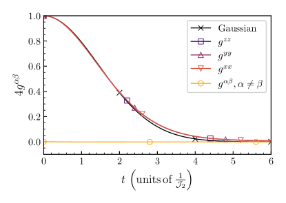
Figure 2: spinDMFT results for the isotropic Heisenberg model with zero magnetic field. The Gaussian fit for short times is best with a standard deviation $\sigma\leavevmode\nobreak\ =\leavevmode\nobreak\ 1.46/\mathcal{J}_{2}$.

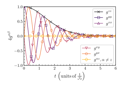
Figure 3: spinDMFT results for the isotropic Heisenberg model with finite magnetic field $\gamma_{\text{s}}B=5.0\,\mathcal{J}_{2}$.

A first validation of spinDMFT consists of the successful check that the derived symmetry relations hold in the framework of spinDMFT. The results of the self-consistency problem (20) for zero and finite magnetic field are depicted in Figs. 2 and 3. The spinDMFT fulfills the symmetry relations for both cases. Moreover, the Larmor precession with frequency $\omega_{\text{L}}\leavevmode\nobreak\ =\leavevmode\nobreak\ \gamma_{\text{s}}\leavevmode\nobreak\ B$ is clearly visible in the transversal components for finite magnetic field.

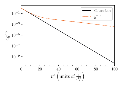
Figure 4: Diagonal autocorrelations on a log-scale for zero magnetic field compared to the Gaussian short-time fit as functions of $t^{2}$.

For short times and zero magnetic field, a Gaussian fit describes $g^{\alpha\alpha}$ very well in the linear plot in Fig. 2. Some deviation is discernible from intermediate times onwards. To analyze this deviation in more detail the functions are plotted in Fig. 4 on a logarithmic scale vs. $t^{2}$. Interestingly, the diagonal autocorrelations appear to show Gaussian behavior at short and at long times, but with different standard deviations. For longer times, the decay is slowed down.

III.3 Comparison to results of other approaches

We compare results from the spinDMFT to results from exact diagonalization (ED), iterated equations of motion (iEoM), and Chebyshev expansion technique (CET). ED is a very well-known technique and the latter two approaches have been explained above. A conceptual difficulty lies in the fact that these alternative techniques work best for small and low-dimensional systems while spinDMFT is rather justified in large, high-dimensional systems. But comparing results from spinDMFT to these alternatives is the best option at hand. Note that such comparisons are particularly challenging for spinDMFT.

Considering the self-consistency problem (20), we stress that all lattice properties are embodied in a single coupling constant, namely the root-mean-square $\mathcal{J}_{2}$. No site index appears because we deal with homogeneous systems. Time is naturally measured in units of $1/\mathcal{J}_{2}$. First, we consider one-dimensional (1D) spin chains with $S={\tfrac{1}{2}}$. For finite pieces of chains with $N$ sites, periodic boundary conditions (PBC) are taken. The Hamiltonian in the isotropic case reads

$$\boldsymbol{H}_{1\text{D}}=J\sum_{i=1}^{N}\vec{\boldsymbol{S}}_{i}\cdot\vec{\boldsymbol{S}}_{i+1},$$ (48)

which entails

$$\mathcal{J}_{2}=\sqrt{2}J.$$ (49)

Figure 5 compares the results from the above mentioned methods to the data obtained from spinDMFT. The ED data are taken from Ref. 59. The results from ED and CET coincide very nicely in the considered time interval. Moreover, no finite-size effects are discernible in this interval. For not too long times, the iEoM result also matches very well. It has the advantage to consider the infinite system by construction. These results almost coincide with the spinDMFT data until roughly $t\approx 3/\mathcal{J}_{2}$. The subsequent deviations can be attributed to the small coordination number of the 1D chain with $z=2$ which, obviously, is a challenge for a mean-field approach.

The spinDMFT shows quick and rather complete decoherence while the genuine 1D results show weak coherent revivals at $t\approx 5/\mathcal{J}_{2}$ and $t\approx 9/\mathcal{J}_{2}$. This is not surprising because the integrable 1D system is strongly constrained in its dynamics due to its extensive number of conserved quantities [60].

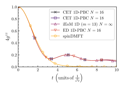
Figure 5: Results for the isotropic diagonal autocorrelation in the 1D Heisenberg chain as calculated by ED, CET, and iEoM compared to the data of spinDMFT. We emphasize that the CET operates on finite cluster systems with periodic boundary conditions (PBC) only. The number of sites considered here is denoted by $N$. The relative error tolerance (33) of each CET time evolution is $\epsilon=$1\text{\times}{10}^{-3}$$.

Figure 6 compares the results of CET and iEoM in 2D, i.e., for the isotropic Heisenberg model on the square lattice

$$\boldsymbol{H}_{2\text{D}}=J\sum_{\langle i,j\rangle}\vec{\boldsymbol{S}}_{i}\cdot\vec{\boldsymbol{S}}_{j}$$ (50)

with NN coupling $J$ to the data obtained from spinDMFT. In this case, $\mathcal{J}_{2}=2J$ holds. The agreement between CET and iEoM is good up to $t\approx 3.5/\mathcal{J}_{2}$; then, the effects of finite loop order $m$ kick in. In 2D, it is unfortunately not possible to reach larger values of $m$. Up to this range, the spinDMFT is in nice agreement with the other approaches as well. What is even more interesting is to see the evolution from 1D to 2D. To this end, we include the CET result in 1D. Clearly, passing from 1D to 2D improves the agreement between the genuine numerical results and spinDMFT. This is exactly what one had to expect in view of the derivation of spinDMFT as mean-field theory which becomes exact for infinite coordination number. Hence, this observation constitutes a good confirmation of the validity of spinDMFT.

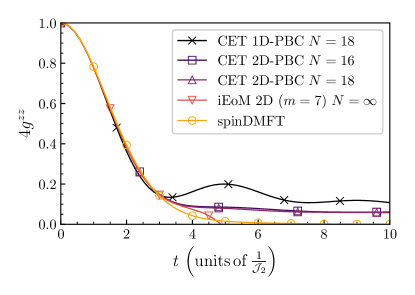
Figure 6: Results for the isotropic diagonal autocorrelation in the 2D Heisenberg square lattice as calculated by CET and iEoM compared to the data of spinDMFT. PBC stands for periodic boundary conditions and $N$ is the number of sites. The relative error tolerance (33) of each CET time evolution is $\epsilon=$1\text{\times}{10}^{-3}$$.

In order to corroborate the foundation of spinDMFT further we consider the Heisenberg model on complete graphs, i.e., graphs where each site is connected to all other sites

$$\boldsymbol{H}_{\text{CG}}=\sum_{i<j}J_{ij}\vec{\boldsymbol{S}}_{i}\cdot\vec{\boldsymbol{S}}_{j}.$$ (51)

Such graphs or clusters are called infinite-range clusters in the physical literature. The Heisenberg model on such graphs is highly symmetric if the coupling is the same for all links. This leads to rather special autocorrelations. In order to avoid features from non-generic high symmetries we consider a random model where the couplings are drawn from a Gaussian distribution. Then, they are normalized, i.e., multiplied by a suitable constant $\lambda_{j}$, such that

$$\mathcal{J}_{2}^{2}=\sum_{i}J_{ij}^{2}$$ (52)

holds for all $j$. The results for the autocorrelations are averaged over 100 sets of random couplings. Figure 7 compares the CET results to the data from spinDMFT for various values of $N$. The symbols display the data extrapolated to $N=\infty$ by a linear fit in $1/N^{3/2}$ of the data for the three largest values of $N$. This particular power law fit is chosen in view of the scaling of each $J_{ij}\propto 1/\sqrt{N}$ stemming from the normalization (52). This suggests to use power law fits $\propto 1/N^{p/2}$ with some integer $p$. We found that $p=3$ is most robust.

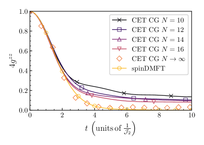
Figure 7: CET results of the isotropic diagonal autocorrelation in the random Heisenberg model on various complete graphs compared to the data of spinDMFT. $N$ is the number of sites. In addition, the extrapolation to $N=\infty$ is shown. The relative error tolerance (33) of each CET time evolution is $\epsilon=$1\text{\times}{10}^{-3}$$.

The obvious trend is that the data for finite $N$ appear to converge to the spinDMFT. This observation again justifies the systematic derivation of the advocated dynamic mean-field theory.

Finally, we mention that the Ising model on complete graphs

$$\boldsymbol{H}_{\text{CG,Ising}}=J\sum_{i<j}{\boldsymbol{S}}_{i}^{z}{\boldsymbol{S}}^{z}_{j},$$ (53)

in the limit $N\to\infty$ has the autocorrelations [61]

$$4g^{xx} =\mathrm{e}^{-\frac{1}{8}\mathcal{J}_{2}^{2}t^{2}}$$ (54a)

$$4g^{zz} =1.$$ (54b)

The energy scale is $\mathcal{J}_{2}=\sqrt{N-1}J$. These results are reproduced by spinDMFT; we refrain from displaying them because the graphs coincide perfectly. Due to the spin anisotropy the self-consistency conditions are changed to

$$\overline{V^{\alpha}(t_{1})V^{\alpha}(t_{2})} =\mathcal{J}_{2}\langle\boldsymbol{S}^{\alpha}(t_{1})\boldsymbol{S}^{\alpha}(t_{2})\rangle \alpha =x,y$$ (55a)

$$\overline{V^{z}(t_{1})V^{z}(t_{2})} =\mathcal{J}_{2}\langle\boldsymbol{S}^{z}(t_{1})\boldsymbol{S}^{z}(t_{2})\rangle$$ (55b)

$$\overline{V^{\alpha}(t_{1})V^{\beta}(t_{2})} =0 \alpha \neq\beta.$$ (55c)

On the basis of the above results, we conclude that spinDMFT is a systematically controlled dynamic mean-field approach to disordered spin systems at infinite temperature which becomes exact for infinite coordination number. It is designed to provide quantitative information of the local spin dynamics. It is a valid approximation for finite coordination numbers which nicely captures essential physics such as rapid decoherence, spin anisotropies, and Larmor precession. Due to the required moderate computational resources it is an attractive tool to understand spin dynamics in various setups. We illustrate this last point by applying spinDMFT to a spin ensemble with dipolar interactions.

IV Application to a dipolar surface spin ensemble

In this section, we want to show that spinDMFT can be adapted to models which describe experimental setups or are very close to experimental questions. We illustrate that spinDMFT can be applied to complex physical situations because of its flexibility and, furthermore, that the resulting numerical task is feasible and does not require excessive compute resources.

The model which we will address is motivated by intensive studies of localized defect spins of electronic origin with $S={\tfrac{1}{2}}$ and a $g$-factor of $g\approx 2$ on diamond surfaces which are observed by NV centers [7, 13, 11]. These spins were seen and examined in recent studies [12, 62, 63]. The precise origin of the defect spins is still a matter of debate although recent progress indicates that they are formed by trapped electrons very close to the surface [64]. They appear to be inhomogeneously distributed over the surface [65, 7, 13]. Driving these spins reduces decoherence in shallow NV centers [66]. The surface spins interact with one another and they are subject to additional, slow noise. The origin of the latter is not yet clarified: nuclear proton spins are candidates [11, 67] which agrees with the importance of the precise chemical and morphological conditions at the surface [65]. A second candidate is phonons which also play a role [63]. In addition, NV centers can also measure the dynamics of ¹³C nuclear spin baths which are distributed three-dimensionally in the bulk of diamonds [68].

Here, we do not aim at describing one of the above exciting experiments in detail, but to address a generic model comprising the essential features. To this end, we consider a random ensemble of localized electronic spins $S={\tfrac{1}{2}}$ on a planar surface interacting by dipolar couplings. Aside from these interactions, the spins are subjected to a global magnetic field as well as to local static magnetic field noise. The latter can be viewed as being generated by slowly fluctuating nuclear spins stemming, for instance, from protons.

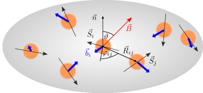
Figure 8: Sketch of the considered dipolar spin ensemble on a planar surface. The magnetic field $B$ (red) defines the $z$-direction; the isotropic random local magnetic fields $\vec{b}_{i}$ (blue) vary in strength and direction from site to site.

IV.1 Model and Definitions

We consider an ensemble of spins $S=\tfrac{1}{2}$ distributed randomly over a planar surface which interact via dipole-dipole interaction. Each spin is subjected to an external magnetic field $\vec{B}$ whose direction defines the $z$ direction which forms an angle $\vartheta$ with the normal $\vec{n}$ of the plane. Additionally, the spins see local random magnetic noise, i.e., local magnetic fields $\vec{b}_{i}$ with zero average. While the system is inhomogeneous we assume that the random distribution is such that each spin sees the same environment on average, i.e., the system behaves on average like a homogeneous system. This means that the average quantities do not depend on the site.

The Hamiltonian is given by

$$\boldsymbol{H} =\sum_{i<j}J\left(R_{ij}\right)\Big{[}(\vec{\boldsymbol{S}}_{i}\cdot\vec{\boldsymbol{S}}_{j})-\frac{3}{R_{ij}^{2}}(\vec{R}_{ij}\cdot\vec{\boldsymbol{S}}_{i})(\vec{R}_{ij}\cdot\vec{\boldsymbol{S}}_{j})\Big{]}$$

$$\qquad+\gamma_{\text{s}}B\sum_{i}\boldsymbol{S}^{z}_{i}+\gamma_{\text{s}}\sum_{i}\vec{b}_{i}\cdot\vec{\boldsymbol{S}}_{i},$$ (56)

where

$$J(R)=\frac{\mu_{0}\gamma_{\text{s}}^{2}}{4\pi R^{3}}.$$ (57)

is the dipolar coupling. We apply spinDMFT which relies on average dynamic mean-fields. Since we want to treat the random local magnetic fields $\vec{b}_{i}$ in addition we have to distinguish three types of averages: (i) the one from spinDMFT which we denote by an overline as before, (ii) the one solely due to the average over the local magnetic fields which we denote by an overline with index ‘n’ for ‘noise’, and (iii) the complete average comprising (i) and (ii) which we denote by an overline with index ‘c’ for ‘complete’.

For simplicity, we assume that the local magnetic fields are distributed isotropically according to a normal distribution defined by the moments

$$\overline{b_{i}^{\alpha}}^{\text{n}} =\mu_{\text{N}}=0, \overline{\left(b_{i}^{\alpha}\right)^{2}}^{\text{n}} =\sigma_{\text{N}}^{2}, \forall i,\alpha.$$ (58)

and

$$\overline{b_{i}^{\alpha}b_{j}^{\beta}}^{\text{n}} =\delta_{ij}\delta_{\alpha\beta}\sigma_{\text{N}}^{2}.$$ (59)

The latter implies that the local fields are independent from one another. The distribution reads as

$$p_{\text{n}}\left(\vec{b}_{i}\right)=\prod_{\alpha}\frac{1}{\sqrt{2\pi\sigma_{\text{N}}^{2}}}\,\text{exp}\left(-\frac{\left(b^{\alpha}_{i}\right)^{2}}{2\sigma_{\text{N}}^{2}}\right).$$ (60)

As mentioned above, we allow for an angle $\vartheta$ between the surface normal $\vec{n}$ and the external magnetic field $\vec{B}$. We introduce the in-plane polar coordinates $R_{ij},\varphi_{ij}$ to express the distance vectors between site $i$ and $j$ by

$$\vec{R}_{ij} =R_{ij}\begin{pmatrix}\cos\left(\varphi_{ij}\right)\\ \sin\left(\varphi_{ij}\right)\cos(\vartheta)\\ \sin\left(\varphi_{ij}\right)\sin(\vartheta)\\ \end{pmatrix}.$$ (61)

The complete system is sketched in Fig. 8 including the various introduced quantities.

IV.2 spinDMFT

As motivated in the previous section where we introduced spinDMFT we define local operators describing the environments of the spins

$$\vec{\boldsymbol{V}}_{i}=\sum_{j\neq i}J\left(R_{ij}\right)\,\underline{\underline{D}}\left(\varphi_{ij},\vartheta\right)\vec{\boldsymbol{S}}_{j},$$ (62)

where the anisotropies are incorporated in the matrix

$$\underline{\underline{D}}\left(\varphi_{ij},\vartheta\right)=\begin{pmatrix}1-3\cos^{2}(\varphi_{ij})&-3\cos(\varphi_{ij})\sin(\varphi_{ij})\cos(\vartheta)&-3\cos(\varphi_{ij})\sin(\varphi_{ij})\sin(\vartheta)\\ -3\cos(\varphi_{ij})\sin(\varphi_{ij})\cos(\vartheta)&1-3\sin^{2}(\varphi_{ij})\cos^{2}(\vartheta)&-3\sin^{2}(\varphi_{ij})\cos(\vartheta)\sin(\vartheta)\\ -3\cos(\varphi_{ij})\sin(\varphi_{ij})\sin(\vartheta)&-3\sin^{2}(\varphi_{ij})\cos(\vartheta)\sin(\vartheta)&1-3\sin^{2}(\varphi_{ij})\sin^{2}(\vartheta)\end{pmatrix}.$$ (63)

With their help, the Hamiltonian can be rewritten

$$\boldsymbol{H}=\frac{1}{2}\sum_{i}\vec{\boldsymbol{S}}_{i}\cdot\vec{\boldsymbol{V}}_{i}+\gamma_{\text{s}}B\sum_{i}\boldsymbol{S}^{z}_{i}+\gamma_{\text{s}}\sum_{i}\vec{b}_{i}\cdot\vec{\boldsymbol{S}}_{i},$$ (64)

where a factor $\frac{1}{2}$ is introduced to avoid double counting.

From the derivation of spinDMFT in Sect. II we know that large coordination numbers provide the justification for this dynamic mean-field theory. Thus, we consider the effective coordination numbers $z$ and $z^{\prime}$ defined in (5) for various lattices and dipolar coupling (57), see Tab. 2.

lattice	$z$	$z^{\prime}$	$z_{\text{NN}}$
triangular	19.1	6.8	6
square	17.5	5.3	4
hexagonal	13.1	3.6	3
rectangular (A)	12.0	2.8	2
rectangular (B)	7.8	2.2	2

Table 2: Effective coordination numbers for various two-dimensional lattices and dipolar coupling $\propto R^{-3}$. The effective coordination numbers were computed taking $4\cdot 10^{6}$ unit cells into account. The conventional coordination number $z_{\text{NN}}$ equals the number of nearest neighbors at each lattice site. For comparison, we include rectangular lattices with the ratios $2:3$ (A) and $1:2$ (B) of their lattice constants in $x$ and $y$ direction, respectively.

As expected, the long range of dipolar interactions increases the effective coordination number to considerably larger values compared to the NN coupling, see for instance the triangular lattice. This effect is larger for $z$ than for $z^{\prime}$ because the sums for higher moments converge faster than those for the second or first moment. We point out that the first moment “just” converges like $\int\frac{RdR}{R^{3}}\propto\frac{1}{R}$.

For randomly distributed spins the issue is more complicated and depends on how the spins are located on the surface. In case of random positions without any restrictions, the effective coordination numbers are fairly small because there is a high probability for each spin to have a single neighbor close to it which dominates $z$ and $z^{\prime}$. We found for completely random distributions $z\approx 1-{10}$. Then, this close partner governs the dynamics and the application of spinDMFT is not well justified. However, considering restrictions for the location of the spins, in particular a minimum distance between the spins, the effective coordination numbers increase substantially to about the values of the triangular lattice which is the closest-packed lattice in two dimensions. We found $z\approx 5-15$. We emphasize that such restrictions are very plausible: a minimum distance can result from the surface structure which does not allow the spin-carrying adatoms to be located very close to one another. In addition, a local repulsion between them would also ensure a minimum distance between the spins. We conclude that the lattice is dense enough so that spinDMFT is justified.

Next, we replace the local-environment fields by dynamic mean-fields

$$\vec{\boldsymbol{V}}_{i}\to\vec{V}_{i}(t)$$ (65)

considering the local mean-field model

$$\boldsymbol{H}_{\text{mf},i}(t)=\vec{V}_{i}(t)\cdot\vec{\boldsymbol{S}}+\gamma_{\text{s}}B\boldsymbol{S}^{z}+\gamma_{\text{s}}\vec{b}_{i}\cdot\vec{\boldsymbol{S}}.$$ (66)

The self-consistency conditions need to be complemented by the effect of the random noise fields $\vec{b}_{i}$. Averaging has to be done over the random time series for $\vec{V}_{i}$ and the random local magnetic fields. We perform this in a single step and thus pass to combined fields

$${\vec{W}}_{i}(t)=\vec{V}_{i}(t)+\gamma_{\text{s}}\vec{b}_{i}$$ (67)

and perform a single average over the combined distribution

$${p}_{i}[{\vec{\mathcal{W}}}_{i}]=\frac{1}{\sqrt{\text{det}2\pi\underline{\underline{M}}_{i}}}\mathrm{e}^{-\frac{1}{2}{\vec{\mathcal{W}}}_{i}^{\top}\underline{\underline{M}}_{i}^{-1}{\vec{\mathcal{W}}}_{i}},$$ (68)

where the modified covariance matrix is given by

$$M_{i}^{\alpha\beta}(t_{1},t_{2}) =\overline{{W}_{i}^{\alpha}(t_{1}){W}_{i}^{\beta}(t_{2})}^{\text{c}}$$ (69a)

$$=\overline{V_{i}^{\alpha}(t_{1})V_{i}^{\beta}(t_{2})}+\gamma_{\text{s}}^{2}\overline{b^{\alpha}_{i}b^{\beta}_{i}}^{\text{n}}.$$ (69b)

Then, the noise leads only to an offset in the second moments which is constant in time.

The self-consistency condition of the first moment is still trivial

$$\overline{{W}^{\alpha}_{i}(t)}^{\text{c}}=\langle\boldsymbol{V}^{\alpha}_{i}(t)\rangle+\gamma_{\text{s}}\overline{b^{\alpha}_{i}}^{\text{n}}=0,\qquad\forall\alpha,i.$$ (70)

For the second moments we consider the self-consistency

$$\overline{V_{i}^{\alpha}(t_{1})V_{i}^{\beta}(t_{2})}=\langle\boldsymbol{V}_{i}^{\alpha}(t_{1})\boldsymbol{V}_{i}^{\beta}(t_{2})\rangle,$$ (71)

and thus the complete self-consistency reads as

$$\overline{W_{i}^{\alpha}(t_{1})W_{i}^{\beta}(t_{2})}^{\text{c}}=\gamma_{\text{s}}^{2}\overline{b^{\alpha}_{i}b^{\beta}_{i}}^{\text{n}}+\sum_{k\neq i}\sum_{\rho\gamma}J^{2}\left(R_{ik}\right)$$ (72)

$$\qquad\quad\times D_{\alpha\rho}\left(\varphi_{ik},\vartheta\right)D_{\beta\gamma}\left(\varphi_{ik},\vartheta\right)\langle\boldsymbol{S}_{k}^{\rho}(t_{1})\boldsymbol{S}_{k}^{\gamma}(t_{2})\rangle^{\text{\tiny{(mf)}}}_{\phantom{\vec{V}}}.$$

This equation still constitutes a challenging numerical issue because it amounts up to a self-consistency condition for each spin. But, as stated at the beginning of Sect. IV.1, we assume that the system is dense enough to be treated on average as a homogeneous system. Essentially, this means that $\mathcal{J}_{2,i}$ takes the same value at each site $i$. Then, the site indices can be omitted and we obtain much simpler self-consistency conditions

$$\overline{W^{\alpha}(t_{1})W^{\beta}(t_{2})} =$$ (73)

$$\mathcal{J}^{2}\sum_{\rho\gamma} \chi^{\alpha\beta}_{\rho\gamma}(\vartheta)\langle\boldsymbol{S}^{\rho}(t_{1})\boldsymbol{S}^{\gamma}(t_{2})\rangle^{\text{\tiny{(mf)}}}+\delta_{\alpha\beta}\gamma_{\text{s}}^{2}\sigma_{\text{N}}^{2}.$$

The constants $\mathcal{J}$ and $\chi^{\alpha\beta}_{\rho\gamma}$ embody the energy scale and the spin anisotropies. The key idea is to approximate the discrete sums in the self-consistency conditions by integrals assuming a continuous distribution of spins with density $n_{0}=1/r^{2}_{\text{min}}$. Of course, this is not exact, but it provides a well-justified quantitative relation between the dipolar interaction in Eq. (57) and the prefactors of the self-consistency condition (IV.2). We replace the sum by the integration

$$\sum_{k\neq i}\approx n_{0}\int_{r_{\text{min}}}^{\infty}\mathrm{d}R\,R\int_{0}^{2\pi}\mathrm{d}\varphi$$ (74)

yielding

$$\mathcal{J}^{2} =2\pi n_{0}\int_{r_{\text{min}}}^{\infty}\mathrm{d}R\,RJ^{2}(R)=\frac{\mu_{0}^{2}\gamma_{\text{s}}^{4}}{32\pi r_{\text{min}}^{6}}$$ (75a)

$$\chi^{\alpha\beta}_{\rho\gamma}(\vartheta) =\frac{1}{2\pi}\int_{0}^{2\pi}\mathrm{d}\varphi\,D_{\alpha\rho}\left(\varphi,\vartheta\right)D_{\beta\gamma}\left(\varphi,\vartheta\right).$$ (75b)

Since we are dealing with a system constant in time we study self-consistent solutions which depend only on the time difference $t_{1}-t_{2}$. Hence, from now on we only consider correlation functions with $t_{1}=t$ and $t_{2}=0$,

$$g^{\alpha\beta}(t) :=\langle\boldsymbol{S}^{\alpha}(t)\boldsymbol{S}^{\beta}(0)\rangle^{\text{\tiny{(mf)}}}$$ (76a)

$$w^{\alpha\beta}(t) :=\overline{{W}^{\alpha}(t){W}^{\beta}(0)}.$$ (76b)

In the remainder of this section, we specialize the above general equations to the case of a perpendicular magnetic field, i.e., $\vartheta=0$, for simplicity. From Eq. (75b) we obtain

$$\chi^{xx}_{xx} =\chi^{yy}_{yy}=\tfrac{11}{8}$$ (77a)

$$\chi^{xy}_{xy} =\chi^{yx}_{yx}=-\tfrac{7}{8}$$ (77b)

$$\chi^{xx}_{yy} =\chi^{yy}_{xx}=\chi^{xy}_{yx}=\chi^{yx}_{xy}=\tfrac{9}{8}$$ (77c)

$$\chi^{xz}_{xz} =\chi^{yz}_{yz}=\chi^{zx}_{zx}=\chi^{zy}_{zy}=-\tfrac{1}{2}$$ (77d)

$$\chi^{zz}_{zz} =1,$$ (77e)

by straightforward analytic calculation while the other coefficients vanish.

For a brief symmetry discussion, we consider the original Hamiltonian (56). Since $\vartheta=0$, the transversal $x$ and $y$ spin components lie in the plane of the surface. Thus, the dipolar interaction term and the magnetic-field term are invariant under a rotation in spin and real space about the angle $\pi/2$ around the $z$ axis. This does not hold true for the noise term $\propto\vec{b}_{i}$. But the noise distribution (60) is isotropic so that on average this term also remains invariant and we have a rotational symmetry of the total system. In particular, this implies

$$g^{xx}(t) =g^{yy}(t)$$ (78a)

$$g^{xy}(t) =-g^{yx}(t)$$ (78b)

$$g^{xz}(t) =g^{zx}(t)=g^{yz}(t)=g^{zy}(t)=0.$$ (78c)

Summarizing, we obtain the self-consistency equations

$$w^{xx}(t) =w^{yy}(t)=\tfrac{5}{2}\mathcal{J}^{2}g^{xx}(t)+\gamma_{\text{s}}^{2}\sigma_{\text{N}}^{2}$$ (79a)

$$w^{xy}(t) =-w^{yx}(t)=-2\mathcal{J}^{2}g^{xy}(t)$$ (79b)

$$w^{xz}(t) =w^{zx}(t)=w^{yz}(t)=w^{zy}(t)=0$$ (79c)

$$w^{zz}(t) =\mathcal{J}^{2}g^{zz}(t)+\gamma_{\text{s}}^{2}\sigma_{\text{N}}^{2}.$$ (79d)

It is worth mentioning that the noise explicitly appears in these equations because we included it in the mean-field $\vec{W}$. The magnetic field, on the other hand, enters the physical problem in the Hamiltonian (66). Another important observation is that the transversal and longitudinal equations (79a) and (79d) show different prefactors. Certainly, this leads to different behavior of the corresponding autocorrelations. For zero magnetic field, where the cross autocorrelations $g^{xy}=-g^{yx}$ vanish due to time reversal symmetry, we expect $g^{xx}=g^{yy}$ to decay slower than $g^{zz}$, since the transversal mean-field is stronger so that the $z$ components are more strongly precessing.

Henceforth, we measure the time in units of $\frac{1}{\mathcal{J}}$ and it makes sense to define a dimensionless noise strength and a dimensionless magnetic field

$$C:=\frac{\gamma_{\text{s}}^{2}\sigma_{\text{N}}^{2}}{\mathcal{J}^{2}}$$ (80a)

$$\widetilde{B}:=\frac{\gamma_{\text{s}}B}{\mathcal{J}}.$$ (80b)

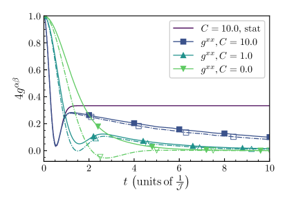
Figure 9: Numerical results of the self-consistency problem (79) for zero magnetic field and various noise strengths. The transversal diagonal autocorrelations $g^{xx}$ (solid line, filled markers) as well as the longitudinal autocorrelations $g^{zz}$ (dashed-dotted line, open markers) are depicted. Moreover, we plotted the analytical result (81) for $C=10.0$ where only the static noise (with subscript ‘stat’) is considered without spin-spin coupling.

Fig. 9 shows the numerical results of the self-consistent equations (79) for various noise strengths and zero magnetic field. Considering $C=0.0$, we observe a clear difference between the transversal and longitudinal signal. This anisotropy is expected due to the different prefactors in (79a) and (79d) as mentioned before. For $C=1.0$, the difference is still present, however, both curves show a similar trend: a local minimum at the beginning followed by a rather slow decay. As we increase $C$, the anisotropy further diminishes because the isotropic noise contributions in (79a) and (79d) dominate more and more over the dipolar terms. In case of a very large noise strength, the mean-field contributions can be neglected and the remaining dynamics can be solved analytically [69, 19]

$$4g^{\alpha\alpha}_{\text{stat}}(t) =\frac{1}{3}\left(1+2\left[1-t^{2}C\mathcal{J}^{2}\right]\mathrm{e}^{-\frac{1}{2}t^{2}C\mathcal{J}^{2}}\right).$$ (81)

Inspecting Fig. 9, the data approach the curve (81) for large values of $C$ and short times. At larger times, i.e., beyond the local minimum, the dynamics due to the dipolar couplings makes itself felt and the signal decays below the analytical plateau. This is not surprising since the analytical consideration only includes static noise neglecting any mean-field dynamics. The corresponding coupling may be weak compared to the noise, but it certainly affects the long-time behavior of the signals.

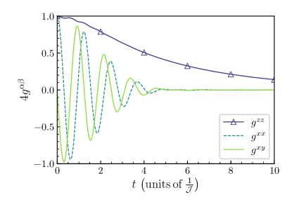
Figure 10: Numerical results of the self-consistency problem (79) for $C=0.0$, $\widetilde{B}=5.0$.

Figs. 10 and 11 show numerical results for finite magnetic field. What catches the eye is that the transversal autocorrelations in both figures show typical Larmor precessions with $\omega_{\text{L}}=\gamma_{\text{s}}B$. For $C=0.0$, the precession persists until the transversal signals have decayed completely. For $C=10.0$, in contrast, the oscillations of $g^{xx}$ disappear very early although the signal is still finite. Subsequently, this correlation shows a slow long-time decay without discernible precession. We attribute this behavior to the presence of transversal noise stabilizing $g^{xx}=g^{yy}$. This noise component is certainly weakened by the longitudinal magnetic field, but it appears to be still strong enough to keep the signal finite for quite a while. Remarkably, the combination of noise and magnetic field causes a slow down of the longitudinal autocorrelation. This behavior is studied in detail in the next section where we use the RWA to tackle the problem for considerably larger magnetic fields. Since the transversal noise vanishes for such large fields, we expect the transversal long-time signal to vanish very quickly.

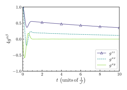
Figure 11: Numerical results of the self-consistency problem (79) for $C=10.0$ and $\widetilde{B}=5.0$.

IV.3 Strong-Field Regime and RWA

In the preceding section, we treated a general external magnetic field of arbitrary strength, weak or strong, but perpendicular to the plane. In this respect, the situation was specific. In the present section, we choose the angle $\vartheta$ of the external field with the surface normal in an arbitrary way, but consider a strong field so that the RWA is valid.

First, we switch from the laboratory frame to the frame rotating with the Larmor frequency of precession

$$\omega_{\text{L}}=\gamma_{\text{s}}B.$$ (82)

This leads to a time-dependent effective Hamiltonian with oscillating terms. They oscillate the faster the stronger the magnetic field is. The RWA consists in averaging these fast oscillations yielding an effective time-independent Hamiltonian again. The spinDMFT is applied to this effective time-independent Hamiltonian. This requires to solve a closed set of self-consistency equations capturing the spin dynamics in the rotating frame.

In order to consider the system in the Larmor rotating frame one has to rotate any observables of the lab frame backwards by the unitary evolution operator

$$\boldsymbol{U}_{\text{Z}}(t,t_{0}):=\mathrm{e}^{\texttt{i}\boldsymbol{H}_{\text{Z}}(t-t_{0})}.$$ (83)

where the Zeeman term is the last-but-one term in Eq. (56):

$$\boldsymbol{H}_{\text{Z}} :=\gamma_{\text{s}}B\sum_{i}\boldsymbol{S}^{z}_{i}.$$ (84)

The spin operators are given in the rotating frame by

$$\boldsymbol{S}^{\alpha}_{i,\text{rot}}(t) =\boldsymbol{U}^{\dagger}_{\text{Z}}(t,t_{0})\boldsymbol{S}^{\alpha}_{i,\text{lab}}(t)\boldsymbol{U}_{\text{Z}}(t,t_{0})$$ (85a)

$$=\boldsymbol{U}^{\dagger}_{\text{Z}}(t,t_{0})\boldsymbol{U}^{\dagger}(t,t_{0})\boldsymbol{S}_{i}^{\alpha}(t_{0})\boldsymbol{U}(t,t_{0})\boldsymbol{U}_{\text{Z}}(t,t_{0}).$$ (85b)

The full time evolution in the rotating frame results from the complete time evolution operator

$$\boldsymbol{U}^{\text{rot}}(t,t_{0}):=\boldsymbol{U}(t,t_{0})\boldsymbol{U}_{\text{Z}}(t,t_{0}).$$ (86)

Its Schödinger equation is derived by inserting (86) in the original Schödinger equation

$$\texttt{i}\partial_{t}\boldsymbol{U}^{\text{rot}}(t,t_{0})=\boldsymbol{H}^{\text{rot}}(t)\boldsymbol{U}^{\text{rot}}(t,t_{0})$$ (87)

with the Hamiltonian

$$\boldsymbol{H}^{\text{rot}}(t)=\boldsymbol{U}_{\text{Z}}(t,t_{0})\left(\boldsymbol{H}-\boldsymbol{H}_{\text{Z}}\right)\boldsymbol{U}^{\dagger}_{\text{Z}}(t,t_{0}).$$ (88)

Clearly, the Zeeman term $\boldsymbol{H}_{\text{Z}}$ in $\boldsymbol{H}$ is canceled in this way which was the goal of this transformation.

The remaining terms, i.e., the dipole interaction and the noise are rotated by $\boldsymbol{U}_{\text{Z}}$. As a consequence, the Hamiltonian $\boldsymbol{H}^{\text{rot}}(t)$ is strongly time-dependent comprising fast oscillating terms such as $\cos(\omega_{\text{L}}t)$ or $\sin(\omega_{\text{L}}t)$ which are averaged in the sense of a Magnus expansion [70] in first order. The neglected terms are smaller by a factor $1/\omega_{\text{L}}$. Put simply, the larger the Larmor frequency $\omega_{\text{L}}$ is relative to the typical dipolar interaction frequency $\omega_{\text{DD}}=\mathcal{J}/\hbar$, the better the RWA is justified. Thus, the strong-field regime is realized for

$$B\gg B_{\text{DD}}=\gamma_{\text{s}}\omega_{\text{DD}}.$$ (89)

In this regime, one replaces all fast oscillating terms in the Hamiltonian by their average values, i.e.,

$$\cos(\omega_{\text{L}}t),\,\sin(\omega_{\text{L}}t) \to 0$$ (90a)

$$\cos(2\omega_{\text{L}}t),\,\sin(2\omega_{\text{L}}t) \to 0.$$ (90b)

In our case, we obtain

$$\boldsymbol{H}^{\text{rot}}=\frac{1}{2}J\left(R_{ij}\right)\sum_{i<j}\left(1-3\sin^{2}(\varphi_{ij})\sin^{2}(\vartheta)\right)\left(2\boldsymbol{S}_{i}^{z}\boldsymbol{S}_{j}^{z}-\boldsymbol{S}_{i}^{x}\boldsymbol{S}_{j}^{x}-\boldsymbol{S}_{i}^{y}\boldsymbol{S}_{j}^{y}\right)+\gamma_{\text{s}}\sum_{i}b_{i}^{z}\boldsymbol{S}_{i}^{z},$$ (91)

which is again time-independent by construction. Note that the transversal components of the magnetic field noise are eliminated while the longitudinal component remains unchanged. Therefore, one expects growing differences between transversal and longitudinal autocorrelations upon increasing the noise strength $\sigma_{\text{N}}$.

Next, spinDMFT is applied to the Hamiltonian (91). We only highlight expressions which differ from the previous application. Expressed in local-field operators, the Hamiltonian reads as

$$\boldsymbol{H}^{\text{rot}} =\frac{1}{2}\sum_{i}\vec{\boldsymbol{S}}_{i}\cdot\vec{\boldsymbol{V}}_{i}+\gamma_{\text{s}}\sum_{i}b_{i}^{z}\boldsymbol{S}_{i}^{z}$$ (92a)

$$\vec{\boldsymbol{V}}_{i} =\sum_{j,j\neq i}J\left(R_{ij}\right)\,\underline{\underline{D}}^{\text{rot}}\left(\varphi_{ij},\vartheta\right)\vec{\boldsymbol{S}}_{j},$$ (92b)

where $\underline{\underline{D}}^{\text{rot}}$ is given by

$$\underline{\underline{D}}^{\text{rot}}(\varphi_{ij},\vartheta) =\left(3\sin^{2}(\varphi_{ij})\sin^{2}(\vartheta)-1\right)\begin{pmatrix}\tfrac{1}{2}&0&0\\ 0&\tfrac{1}{2}&0\\ 0&0&-1\\ \end{pmatrix}.$$ (93)

Replacing the local-field operators by the corresponding mean-fields leads to the local mean-field Hamiltonian

$$\boldsymbol{H}^{\text{rot}}_{\text{mf},i}=\vec{V}_{i}(t)\cdot\vec{\boldsymbol{S}}+\gamma_{\text{s}}b_{i}^{z}\boldsymbol{S}^{z}$$ (94)

and we again combine noise and mean-field in

$${\vec{W}}_{i}(t)=\vec{V}_{i}(t)+\gamma_{\text{s}}\vec{e}_{z}b_{i}^{z},$$ (95)

since both follow from Gaussian distributions. While the first moment is still zero, the second moments obey

$$w^{\alpha\beta}(t_{1}-t_{2}): =\overline{{W}^{\alpha}(t_{1}){W}^{\beta}(t_{2})}$$ (96a)

$$=\delta_{\alpha\beta}\delta_{\alpha z}\gamma_{\text{s}}^{2}\sigma_{\text{N}}^{2}$$ (96b)

$${+}\sum_{\rho\gamma} \mathcal{J}^{2}\left(\chi^{\text{rot}}\right)^{\alpha\beta}_{\rho\gamma}(\vartheta)\langle\boldsymbol{S}^{\rho}(t_{1})\boldsymbol{S}^{\gamma}(t_{2})\rangle^{\text{\tiny{(mf)}}}.$$

The coupling $\mathcal{J}$ is given by Eq. (75a) and the coefficients $\chi^{\text{rot}}$ result from Eq. (75b) with $\underline{\underline{D}}$ replaced by $\underline{\underline{D}}^{\text{rot}}$.

Defining the function of the polar angle $\vartheta$

$$I(\vartheta) :=\frac{1}{2\pi}\int_{0}^{2\pi}\mathrm{d}\varphi\,\left(1-3\sin^{2}(\varphi)\sin^{2}(\vartheta)\right)^{2}$$ (97a)

$$=\frac{27}{8}\sin^{4}(\vartheta)-3\sin^{2}(\vartheta)+1,$$ (97b)

we can express the prefactors concisely by

$$\left(\chi^{\text{rot}}\right)^{xx}_{xx} =\left(\chi^{\text{rot}}\right)^{yy}_{yy}=\tfrac{1}{4}I(\vartheta)$$ (98a)

$$\left(\chi^{\text{rot}}\right)^{xy}_{xy} =\left(\chi^{\text{rot}}\right)^{yx}_{yx}=\tfrac{1}{4}I(\vartheta)$$ (98b)

$$\left(\chi^{\text{rot}}\right)^{xz}_{xz} =\left(\chi^{\text{rot}}\right)^{yz}_{yz}=-\tfrac{1}{2}I(\vartheta)$$ (98c)

$$\left(\chi^{\text{rot}}\right)^{zx}_{zx} =\left(\chi^{\text{rot}}\right)^{zy}_{zy}=-\tfrac{1}{2}I(\vartheta)$$ (98d)

$$\left(\chi^{\text{rot}}\right)^{zz}_{zz} =I(\vartheta).$$ (98e)

Any other coefficient vanishes because $\underline{\underline{D}}^{\text{rot}}$ is diagonal.

We reconsider the symmetries of the underlying system to be able to formulate the minimum set of self-consistency conditions. The original rotating-frame Hamiltonian (91) is invariant under spin rotation around the $z$ axis by construction: all transversal spin components only occur in pairs. The dipolar part is invariant under time reversal. While this does not hold for the noise term for each individual $\vec{b}_{i}$, their distribution remains unchanged under time reversal. Spin-rotation symmetry and time-reversal symmetry allow us to conclude

$$g^{xx}(t) =g^{yy}(t)$$ (99a)

$$g^{\alpha\beta}(t) =0, \alpha \neq\beta.$$ (99b)

This enables us to reduce the general self-consistency conditions (96) to

$$w^{xx}(t) =w^{yy}(t)=\tfrac{1}{4}\mathcal{J}^{2}I(\vartheta)g^{xx}(t)$$ (100a)

$$w^{\alpha\beta}(t) =0, \alpha \neq\beta$$ (100b)

$$w^{zz}(t) =\mathcal{J}^{2}I(\vartheta)g^{zz}(t)+\gamma_{\text{s}}^{2}\sigma_{\text{N}}^{2}.$$ (100c)

Note that there is a natural anisotropy between the transversal and longitudinal equation again, but this time by a factor of four. Furthermore, the noise only acts in the $z$-direction. Considering the results of the previous section, we expect even bigger differences between the autocorrelations here. Henceforth, we no longer use the terms “diagonal” and “cross” because no cross autocorrelations appear in the RWA dipole model. If not stated otherwise, we set $\vartheta$ to the so-called magic angle

$$\vartheta_{\text{magic}} :=\arcsin\sqrt{\frac{2}{3}}$$

$$I(\vartheta_{\text{magic}}) =\frac{1}{2}$$

in our numerical calculations.

Figs. 12 and 13 show our numerical findings for the solutions of the self-consistent equations. Analyzing them, we conclude two important facts:

• Because of the natural anisotropy and the noise, the longitudinal signal decays considerably slower than the transversal signal. Increasing the noise strength amplifies this difference.

• The transversal signal decays very accurately following a Gaussian, while the longitudinal decay is weaker than exponential.

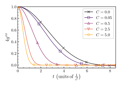
Figure 12: Transversal RWA results of the self-consistency problem (100) for various noise strengths.

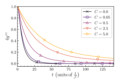
Figure 13: Longitudinal RWA results of the self-consistency problem (100) for various noise strengths.

Considering the results, the first statement is rather obvious. For $C=0.0$, the longitudinal signal already survives significantly longer than the transversal one due to the anisotropic factors in (100). Increasing the noise strength causes the spin to precess more and more quickly and randomly about the $z$ axis. As a result, the transversal spin components experience an even stronger decoherence than before and the corresponding autocorrelations decay faster. In contrast, the $z$ component of the spin is stabilized by the additional rotations about the $z$ axis so that the longitudinal signal relaxes only very slowly. Fig. 14 schematically illustrates the behavior of the spins.

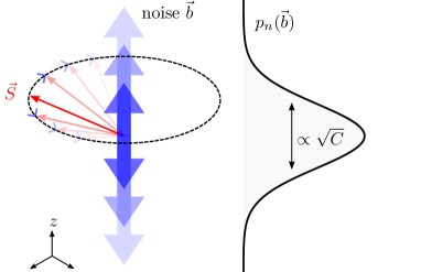
Figure 14: Illustration of a spin subjected to a Gaussian noise in $z$ direction. As the speeds of rotation of the transversal components fluctuate more strongly upon increasing noise strength $C$ the transversal components vanish more rapidly. In return, this weakens the processes which destroy the longitudinal component so that it is stabilized.

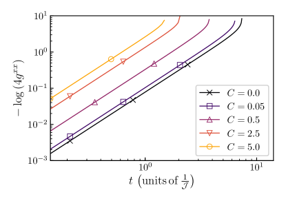
Figure 15: Logarithmic representation of the transversal RWA results for various noise strengths.

To corroborate the statement (ii), Fig. 15 shows the transversal signal in loglog vs. log representation for various noise strengths. All of the results show a linear behavior with a small upward curvature at the end. A closer observation of the curvature reveals that the autocorrelations fall slightly below zero just before they finally converge to zero. We emphasize that this negative dip is only very small, $\propto 10^{-3}$, and hence not visible in the provided figures. Still, we ensured that it does not result from numerical inaccuracies. Interestingly, its height decreases upon increasing the noise width.

The clearly linear behavior in the plot has a slope $r=2$ so that it clearly indicates Gaussian behavior. Hence, we use the fit function

$$4g^{xx}_{\text{Gauss}}(t) =\mathrm{e}^{-\frac{t^{2}}{2\sigma^{2}}}$$ (101)

to extract the standard deviation $\sigma$ as function of the noise strength displayed in Fig. 16.

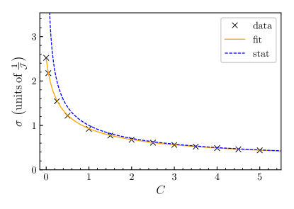
Figure 16: Standard deviations obtained from fitting the transversal signals versus the noise strengths. The dashed blue line is the analytical prediction based on purely static noise, see Eq. (103). The orange line results from a data fit according to (104).

This behavior can be understood by an analytical consideration [69, 19]. We consider purely static noise neglecting the mean-field contributions in the RWA Hamiltonian (94):

$$\boldsymbol{H} =\gamma_{\text{s}}b_{i}^{z}\boldsymbol{S}^{z},$$ (102)

The analytical averaging yields the transversal signal

$$4g^{xx}_{\text{N}}(t) =\mathrm{e}^{-\frac{t^{2}}{2\sigma(C)^{2}}}$$ (103a)

$$\sigma(C) =\frac{1}{\mathcal{J}\sqrt{C}},$$ (103b)

which explains the Gaussian behavior of the transversal signal for large values of $C$. The analytical standard deviation is also depicted in Fig. 16 as blue dashed line. For increasing noise strength it describes the fitted data better and better. This is expected because the larger the static noise is relative to the mean-fields, the better the static noise model captures the dynamics. For small values of $C$ and in particular for $C=0.0$, the transversal signal still follows a Gaussian to good accuracy. The mean-field contribution changes the standard deviations; quite unexpectedly the mean-fields appear to counteract the static noise partly reducing the standard deviation. It turns out that this effect is well captured by the fit

$$\sigma_{\text{fit}}(C) =\frac{1}{\mathcal{J}\sqrt{C+R}}$$ (104)

as can be seen in Fig. 16 with

$$R =$0.159(1)$$$ (105)

This quantifies the contribution of the mean-fields to the transversal spin dynamics.

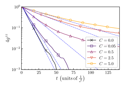
Figure 17: Logarithmic representation of the longitudinal correlation for various noise strengths. The blue dashed-dotted lines correspond to exponential functions with $f(t)=A\mathrm{e}^{-\alpha t}$. They illustrate that the correlations show a positive curvature and thus decay weaker than exponentially.

The behavior of the longitudinal autocorrelations is more complex; Fig. 17 shows that the decay is weaker than exponentially as we stated before. We refer to Sect. IV.5 for a detailed examination of the behavior.

IV.4 Transition from weak to strong external magnetic field

If we consider the case of a surface perpendicular to the external magnetic field, i.e., $\vartheta=0$, we can compare the results from Sect. IV.2 for arbitrarily strong magnetic fields to the results from the previous Sect. IV.3 based on the RWA. This allows us to study how well the RWA reproduces the exact result. In particular, we can determine above which magnetic fields the RWA is reliable and to which extent. First, we compute the results of the self-consistency problem in the lab frame (exact spinDMFT) (79) and in the Larmor rotating frame using RWA (RWA spinDMFT) (100). Then, we transform the exact spinDMFT results to the Larmor rotating frame via

$$g_{\text{rf}}^{xx}(t) =g^{xx}(t)\cos(\omega_{\text{L}}t)-g^{xy}(t)\sin(\omega_{\text{L}}t),$$ (106a)

$$g_{\text{rf}}^{xy}(t) =g^{xy}(t)\cos(\omega_{\text{L}}t)+g^{xx}(t)\sin(\omega_{\text{L}}t),$$ (106b)

$$g_{\text{rf}}^{zz}(t) =g^{zz}(t),$$ (106c)

so that a quantitative comparison is possible.

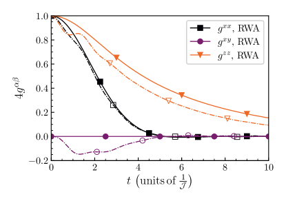
Figure 18: Comparison of the RWA spinDMFT results (solid line, filled markers) with the exact spinDMFT results (dashed-dotted line, open markers) for a small dimensionless magnetic field $\widetilde{B}=2.0$ in the rotating frame at zero static noise $C=0.0$.

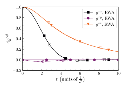
Figure 19: Same as Fig. 18 for moderate dimensionless magnetic field $\widetilde{B}=10.0$.

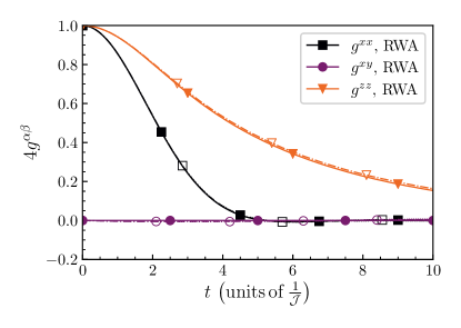
Figure 20: Same as Fig. 18 for large dimensionless magnetic field $\widetilde{B}=50.0$.

In Fig. 18 ($C=0.0$, $\widetilde{B}=2.0$), we observe considerable deviations between both approaches, especially in $g^{xy}$ and $g^{zz}$: due to the moderately large magnetic field, the exact results show deflections and shifts which are not present in RWA. Considering Fig. 19 ($C=0.0$, $\widetilde{B}=10.0$), these deviations clearly shrink upon increasing magnetic field. The deviations from the RWA are difficult to discern. They appear most strongly in $g^{xy}$. As we raise $\widetilde{B}$ further, see Fig. 20 ($C=0.0$, $\widetilde{B}=50.0$), the deviations due to RWA are not visible anymore. The tiny shift between both results for the longitudinal autocorrelation only stems from the discretization of time. It is a purely numerical effect which grows with $\widetilde{B}$.

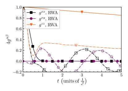
Figure 21: Same as Fig. 18 for finite static noise $C=10.0$ and small dimensionless magnetic field $\widetilde{B}=2.0$.

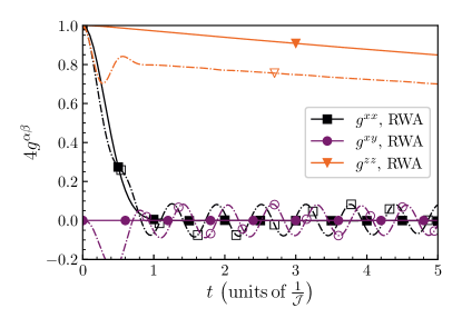
Figure 22: Same as Fig. 18 for finite static noise $C=10.0$ and moderate dimensionless magnetic field $\widetilde{B}=10.0$.

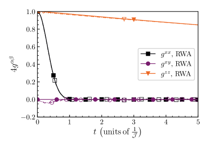
Figure 23: Same as Fig. 18 for finite static noise $C=10.0$ and large dimensionless magnetic field $\widetilde{B}=50.0$.

If static noise is included, see Fig. 21 for $C=10.0$, $\widetilde{B}=2.0$, we observe large deviations for all autocorrelations, even more than what we showed in Fig. 18. The exact transversal results strongly oscillate in contrast to the RWA results and a huge shift between the two curves for the longitudinal autocorrelations occurs. This implies that the presence of static noise requires larger magnetic fields for the RWA to be justified. Figures 22 ($C=10.0$, $\widetilde{B}=10.0$) and 23 ($C=10.0$, $\widetilde{B}=50.0$) confirm this conclusion displaying better and better agreement between the results of both approaches. We argue that this behavior is physically highly plausible because the RWA is justified if the energy scale of the magnetic field is larger than the energy scales of any other interaction in the system, including the static noise.

IV.5 Long-time behavior

Now, we come back to the long-time behavior of the longitudinal autocorrelation. This is an interesting issue because various ideas exist on the origin of the rather slow decay and its functional form [71].

Fig. 17 shows that the autocorrelations do not decay in a Gaussian fashion at all. Such decay would have led to a negative curvature downwards. Instead we discern a positive curvature upwards which implies that the decay is even slower than exponential. The question arises which functional dependencies describe this decay. Considering this, our most successful fitting attempt is a power law according to

$$4g^{zz}_{\text{fit:B}}(t) =Bt^{-m}$$ (107)

with parameters $B$ and $m$. We checked also stretched exponentials since these were suggested in Ref. [71]. But we did not achieve satisfactory fits for an ansatz according to

$$4g^{zz}_{\text{fit:A}}(t) =A\mathrm{e}^{-\alpha t^{\nu}}$$ (108)

with parameters $A$, $\alpha$, and the exponent $\nu$. The longitudinal results including the power law fits can be seen in Fig. 24. Note that much longer times are not easily accessible for two reasons. First, the numerical effort increases as $t^{2}$ for the Monte-Carlo simulation and as $t^{3}$ for the diagonalization. Second, the smaller the autocorrelation is the more difficult it becomes to determine it with good relative accuracy in view of the statistical way of computing it. This is also the reason why we cannot go to longer times for $C\approx 0$.

The exponent $m$ displays a pronounced dependence on the relative noise strength $C$ as depicted in Fig. 25. The dependence $m(C)$ can be described heuristically by

$$m_{\text{fit}}(C) =m_{0}+\frac{k}{C^{r}}.$$ (109)

This fit works surprisingly well in spite of the divergence for $C\to 0$. Limited by the numerical accuracy, we can hardly say if we actually obtain this divergence or if it can be truncated, e.g., by replacing $C\to C+C_{0}$ in (109). This issue is associated to the question if the power law behavior solely results from the presence of the noise or if it is a valid feature of spinDMFT.

All in all, these results provide evidence that the longitudinal autocorrelations are relatively long-lived. Clearly, their long-time behavior poses an interesting question which calls for further research, both numerical and analytical.

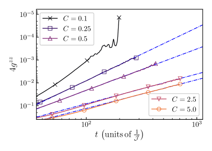
Figure 24: Numerical long-time results of the longitudinal autocorrelations in RWA for various noise strengths in Log vs. Log representation. The blue dashed-dotted lines correspond to power law fits as in (107).

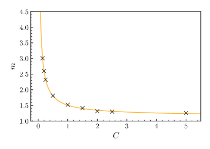
Figure 25: Fitted exponent $m$ from the fit of the longitudinal autocorrelations (107) vs. the noise strength and a fit (orange) as in (109). The estimated parameters are $m_{0}=$1.15(2)$$, $k=$0.35(2)$$ and $r=$0.87(3)$$.

V Conclusions

In this paper, we introduced and justified a mean-field theory designed to capture the spin dynamics in disordered dense spin systems. The key idea is that it is not sufficient to introduce a static mean-field but that the mean-field is dynamic itself so that we call it “spin dynamic mean-field theory” (spinDMFT). As usual, this approach becomes exact if each site has an infinite number of interaction partners, i.e., the coordination number becomes infinitely large. Historically, the same limit led to the introduction of the fermionic dynamic mean-field theory [72, 44].

For spins, we established that the important correlations are the autocorrelations and that these define the dynamic mean-fields to which each spin is subjected. These mean-fields are normally distributed and the dynamic variances of these normal distributions are given by the autocorrelations. This constitutes the self-consistency problem which has to be solved for spinDMFT. We showed how this can be done stochastically.

If the effective single-site problem is linear in the spin operators it does not matter whether we consider classical spins averaged over all directions or a quantum spin given that the average length is scaled to be the same. In this sense, the quantum spin system and the classical spin system have the same spinDMFT. For spin-$1/2$ this has to be the case since locally only linear spin operators can appear. For larger spins, however, higher powers may arise such as anisotropies of various kinds. Then, the quantum spinDMFT and the classical spinDMFT are different.

We gauged the advocated spinDMFT against numerical results for isotropic spin systems obtained by other methods, namely exact diagonalization, iterated equations of motion, and Chebyshev expansion. This can only be done for rather small spin clusters in low dimensions so that the reproduction of the results by spinDMFT is particularly challenging. Nevertheless, encouraging agreement could be established.

Subsequently, we applied spinDMFT to a two-dimensional ensemble of spins with dipolar interactions including local static noise, i.e., fluctuations of magnetic fields. This underlines that spinDMFT is capable of dealing with anisotropic interactions of long range as well. We studied the case of an arbitrary external magnetic field perpendicular to the plane of spins and the RWA for a large tilted magnetic field. For zero tilt, we compared both approaches quantitatively. This allowed us to show quantitatively to which extent the RWA is justified and above which magnetic field it yields reliable results.

We showed that the transversal autocorrelations behave essentially like Gaussians in time. The longitudinal autocorrelations, however, display a more complex behavior with a rather slow decay towards long times. Evidence for power law behavior is found. This certainly calls for further investigations.

We are confident that spinDMFT can be applied successfully to many more physical systems aside from the ones that we mentioned so far. Ample applications can be found for nuclear magnetic resonance (NMR), electron spin resonance (ESR), quantum information storage and processing based on spins in solid state systems, in particular in nanostructures, and for all phenomena related to spin diffusion in such systems.

Conceptually, further issues to be addressed are the treatment of explicitly time-dependent Hamiltonians and spatially inhomogeneous solutions with distributions of mean-fields which vary along the samples. Both extensions are of greatest interest, for example in the coherent control of spin degrees of freedom.

A third fascinating issue consists in an extension of spinDMFT to finite temperatures. So far, we derived the approach for disordered ensembles. But in view of related developments for spin glasses [47, 48] and the general analogy between real and imaginary timess a dynamic mean-field theory for spins at finite temperatures should also exist. Its development would enhance the applicability of spinDMFT even further.

Appendix A Dynamic spin correlations on a Bethe lattice at infinite temperature

The aim of this appendix is to derive the scaling of the correlations as function of the coordination number. This is a tremendous task on arbitrary lattices, even at infinite temperature. Therefore, we consider the Bethe lattice [73] with nearest neighbor coupling between spins $S=\tfrac{1}{2}$, i.e., a Cayley tree of infinite depth, so that each site has the same environment and the system is homogeneous. The coordination number is $z$ and hence the so-called branching ratio is $z-1$. First, we consider the spin-spin correlation. Second, we deduce further correlations. We take the results for the Bethe lattice as representative for more general lattices including long-range interactions leading to large effective coordination numbers.

A.1 Spin-spin correlations

We want to show that the two-time pair correlation functions $\langle\boldsymbol{S}_{i}^{\alpha}(t_{1})\boldsymbol{S}_{j}^{\beta}(t_{2})\rangle$ for $i\neq j$ are suppressed for $z\to\infty$. This property is required to justify the use of the central limit theorem in II.3 and to treat the dynamics of the local fields as independent from the dynamics of a single spin. Mostly, we set $j=0$ and $t_{2}=0$ without loss of generality. The advantage of considering the Bethe lattice is that the shortest distance between any pair of sites is unique because the lattice does not have any loops except self-retracing paths. We consider the general Hamiltonian

$$\boldsymbol{H}_{\text{BL}} =\frac{1}{\sqrt{z}}\sum_{\langle i,j\rangle}\sum_{\alpha\beta}J^{\alpha\beta}\boldsymbol{S}^{\alpha}_{i}\boldsymbol{S}^{\beta}_{j}$$ (110)

with arbitrary couplings $J^{\alpha\beta}=J^{\beta\alpha}$ allowing for spin anisotropy. The factor $z^{-\frac{1}{2}}$ is denoted separately to explicitly keep track of the scaling with $z$. It must be chosen in this way to keep the energy scale of the dynamics, $\mathcal{J}_{2}$ in Eq. (4), constant for $z\to\infty$.

The argument runs as follows. First, we use the Heisenberg equations of motion to set up a system of differential equations for the temporal evolution of the correlation functions. Second, we postulate the scaling of the correlations. Third, we show that the postulated scaling is consistent with the initial conditions and with the differential equations, i.e., the scaling is fulfilled by the initial conditions at $t=0$ and by the differential equations. As starting point, we calculate the time derivative of the general pair correlation function,

$$\frac{\mathrm{d}}{\mathrm{d}t}\langle\boldsymbol{S}^{\rho}_{k}(t)\boldsymbol{S}^{\gamma}_{0}(0)\rangle=\texttt{i}\langle\mathcal{L}\boldsymbol{S}^{\rho}_{k}(t)\boldsymbol{S}^{\gamma}_{0}(0)\rangle$$ (111a)

$$\quad=\frac{-1}{\sqrt{z}}\sum_{j,\langle j,k\rangle}\sum_{\alpha\beta\varphi}J^{\alpha\beta}\epsilon_{\beta\rho\varphi}\langle\boldsymbol{S}^{\alpha}_{j}(t)\boldsymbol{S}^{\varphi}_{k}(t)\boldsymbol{S}^{\gamma}_{0}(0)\rangle,$$ (111b)

where the Levi-Civita tensor occurs due to the spin algebra. The complexity of the expectation value is increased by the Liouville operator $\mathcal{L}$ which consists in the commutation with the Hamiltonian. This leads to an an additional time-dependent spin operator in the expectation value.

The same behavior is observed for higher derivatives: the application of $\mathcal{L}$ results in expectation values with incremented or decremented number of spin operators by one. The decrement occurs if the additionally generated spin operator hits an already present spin operator at the same site and of the same component due to $(\boldsymbol{S}^{\alpha})^{2}=1/4$. The quickly growing number of products of spin operators makes the book keeping tedious. A solution consists in considering the correlation function of a general cluster at time $t$ with a single spin at time $0$ and site $0$

$$g^{\gamma}(\boldsymbol{C},t):=\langle\boldsymbol{C}(t)\boldsymbol{S}_{0}^{\gamma}(0)\rangle.$$ (112)

Here, $\boldsymbol{C}$ denotes an arbitrary product of spin operators at different sites

$$\boldsymbol{C}:=\boldsymbol{C}(c,\alpha)=\prod_{r\in c}\boldsymbol{S}^{\alpha_{r}}_{r}$$ (113)

where $c$ is a set of lattice sites $r\in\{0,...,N\}$ and $\alpha$ is a set of components $\alpha_{r}\in\{x,y,z\}$. The time derivative of such cluster correlations (112) reads

$$\frac{\mathrm{d}}{\mathrm{d}t}g^{\gamma}(\boldsymbol{C},t)=\frac{1}{\sqrt{z}}\sum_{\boldsymbol{C}^{\prime}}J(\boldsymbol{C},\boldsymbol{C}^{\prime})g^{\gamma}(\boldsymbol{C}^{\prime},t),$$ (114)

where the sum runs over all clusters $\boldsymbol{C}^{\prime}$ that can be reached from $\boldsymbol{C}$ by one application of the Liouville operator. All factors that are independent of the coordination number, e.g., the couplings $J^{\alpha\beta}$ and factors $1/4$ from products of the same spin operators, are collected in $J(\boldsymbol{C},\boldsymbol{C}^{\prime})$. Hence, this generalized coupling $J(\boldsymbol{C},\boldsymbol{C}^{\prime})$ does not contribute to the scaling which we want to determine.

By (114) we have formally defined the system of differential equations describing the dynamics of all cluster correlation functions. The starting conditions read as

$$g^{\gamma}(\boldsymbol{C},0) =0, \forall\ \boldsymbol{C} \neq\boldsymbol{S}^{\gamma}_{0},$$ (115a)

$$g^{\gamma}(\boldsymbol{S}^{\gamma}_{0},0) =\frac{1}{4}.$$ (115b)

It is challenging to keep track of the more and more complex clusters. To this end, we define a measure of the cluster size or complexity and link it to the scaling. Since $S=\tfrac{1}{2}$, at each site $r$ of a cluster the active operator can be the identity or one of the three spin components. All products with more factors can be reduced to this case. We call a site “occupied” if one of the three spin components is present at this site. Otherwise, we call it “unoccupied”. We introduce the measure $\kappa(c)$ which consists of two components

$$\kappa(c):=\kappa_{1}(c)+\kappa_{2}(c).$$ (116)

The first term $\kappa_{1}(c)$ measures the overall size of the cluster $c$. Consider a covering of the minimum number of bonds needed to link all sites in $c$ and the origin $0$, see the green bold links in Fig. 26. We stress that this covering is unique, i.e., there is only one such covering due to the properties of the Bethe lattice where two sites are linked by one specific path. There are no loops except self-retracing paths. The second term $\kappa_{2}(c)$ counts the number of empty, unoccupied sites which are touched by this covering.

Figure 26: Cutout of a Bethe lattice with $z=3$. As an example we consider a cluster of four spin operators situated at the filled dots representing occupied sites. The open dots represent empty sites; their number defines $\kappa_{2}(c)=3$. The covering of the cluster is defined by the green links; their number defines $\kappa_{1}=6$ so that $\kappa=9$.

We show below that $\kappa(c)$ is a lower bound for the minimum number $n(\boldsymbol{C})$ of applications of the Liouville operator $\mathcal{L}$ needed to generate $\boldsymbol{C}(c,\alpha)$ from an initial cluster $\boldsymbol{C}_{0}(\{0\},\alpha_{0})$ with a single spin operator $\boldsymbol{S}_{0}^{\alpha_{0}}$ at the origin. For the sake of completeness, we mention that in the exceptional cases

$$\boldsymbol{C} =\boldsymbol{S}^{\rho}_{0}, \rho \neq\gamma,$$ (117)

$n=\kappa(c)+2=2$ holds for reaching $\boldsymbol{S}^{\rho}_{0}$ from $\boldsymbol{S}^{\gamma}_{0}$. From the assertion $n(\boldsymbol{C})\gtrapprox\kappa(c)$ and the starting conditions (115) we deduce

$$\frac{\mathrm{d}^{n}}{\mathrm{d}t^{n}}g^{\gamma}(\boldsymbol{C},t)\Bigr{\rvert}_{t=0} =0, \forall\;n <\kappa(c).$$ (118)

This motivates our central assertion that the cluster correlation functions are scaling with $z$ according to

$$g^{\gamma}(\boldsymbol{C},t)\propto z^{-\frac{\kappa(c)}{2}}.$$ (119)

Obviously, this agrees with the starting conditions

$$g^{\gamma}(\boldsymbol{S}^{\gamma}_{0},0)=\frac{1}{4}\propto z^{0},$$ (120)

while all other cluster correlation functions vanish at $t=0$.

To validate the claim (119) for arbitrary times, we show that it is consistent with the equations of motion (114). A single application of the Liouville operator $\mathcal{L}$ to a cluster $\boldsymbol{C}$ generates a sum of multiple clusters $\boldsymbol{C}^{\prime}$. Since we consider nearest-neighbor interaction, each of these clusters $\boldsymbol{C}^{\prime}$ differs from $\boldsymbol{C}$ only at one link $(i,j)$ where $i$ and $j$ are adjacent. Therefore, it is sufficient to study the possible processes on this link

$$\boldsymbol{C}_{(i,j)}\stackrel{{\scriptstyle\mathcal{L}}}{{\longrightarrow}}\boldsymbol{C}^{\prime}_{(i,j)}$$ (121)

where we denote the subcluster of $\boldsymbol{C}$ or $\boldsymbol{C}^{\prime}$ on this link by $\boldsymbol{C}_{(i,j)}$ and $\boldsymbol{C}^{\prime}_{(i,j)}$, respectively.

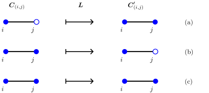
Figure 27: Possible link processes for a single application of $\mathcal{L}$ and their effect on the occupation of the involved sites.

Fig. 27 shows how the effect of $\mathcal{L}$ on the link

$$[\boldsymbol{H}_{\text{BL},(i,j)},\boldsymbol{C}_{(i,j)}]=\sum\boldsymbol{C}^{\prime}_{(i,j)}$$ (122)

can be categorized in three different types. The relevant commutators read as

$$[\boldsymbol{S}_{i}^{\alpha}\boldsymbol{S}_{j}^{\beta}\,,\,\boldsymbol{S}_{i}^{\rho}] =\texttt{i}\epsilon_{\alpha\rho\omega}\boldsymbol{S}_{i}^{\omega}\boldsymbol{S}_{j}^{\beta}$$ (123a)

$$[\boldsymbol{S}_{i}^{\alpha}\boldsymbol{S}_{j}^{\beta}\,,\,\boldsymbol{S}_{i}^{\rho}\boldsymbol{S}_{j}^{\beta}] =\frac{\texttt{i}}{2}\epsilon_{\alpha\rho\omega}\boldsymbol{S}_{i}^{\omega}$$ (123b)

$$[\boldsymbol{S}_{i}^{\alpha}\boldsymbol{S}_{j}^{\beta}\,,\,\boldsymbol{S}_{i}^{\rho}\boldsymbol{S}_{j}^{\delta}] =0.$$ (123c)

Interestingly, the last commutator yields zero for $S=\tfrac{1}{2}$, so that this process does not contribute. The remaining two processes (a) and (b) are analyzed further. Since $\kappa(c)$ depends on the covering of $c$, we distinguish whether the considered link $(i,j)$ is part of this covering or not. This leads to two subcases for processes (a) and (b) as shown in Fig. 28.

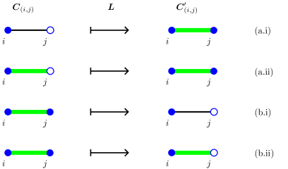
Figure 28: Relevant link processes for a single application of $\mathcal{L}$ including the effect on the covering which is shown in green.

As an example, we derive that the first process (a.i) preserves the asserted scaling. The extension of the covering by one link leads to

$$\kappa_{1}(c^{\prime}) =\kappa_{1}(c)+1$$ (124)

while the number of unoccupied sites remains the same

$$\kappa_{2}(c^{\prime}) =\kappa_{2}(c).$$ (125)

In order to assess the complete scaling one has to count how often a process can occur. We call this its multiplicity $m(c,z)$. The multiplicity of process (a.i) can be bounded from above by counting at maximum $z$ neighbors of each occupied site in $c$. There are $\kappa_{1}(c)-\kappa_{2}(c)+1$ of such sites so that

$$m(c,z)\leq z(\kappa_{1}(c)-\kappa_{2}(c)+1)$$ (126)

holds. The indicators $\kappa_{i}$ depend on the size of the cluster, but not on the coordination number so that the scaling resulting from the differential equation (114) is

$$g^{\gamma}(\boldsymbol{C}^{\text{(a.i)}},t) \propto z^{-\frac{1}{2}}m(c,z)z^{-\frac{\kappa(c^{\prime})}{2}}$$ (127a)

$$\propto z^{-\frac{\kappa(c)}{2}}$$ (127b)

$$\propto g^{\gamma}(\boldsymbol{C},t),$$ (127c)

where $g^{\gamma}(\boldsymbol{C}^{\text{(a.i)}},t)$ denotes the sum of the contributions of the clusters $\boldsymbol{C}^{\prime}$ to the correlation of cluster $\boldsymbol{C}$ via the link process (a.i). Clearly, the asserted scaling of $g^{\gamma}(\boldsymbol{C},t)$ is confirmed. Note that the first factor $z^{-\frac{1}{2}}$ in (127a) stems from the overall scaling on the right hand side of Eq. (114). In conclusion, we showed that the first process is consistent with the claimed scaling (119).

process $(x.y)$	$\kappa_{1}$	$\kappa_{2}$	$m(c,z)\propto$	$g^{\gamma}(\boldsymbol{C}^{\text{(x.y)}},t)\propto$
(a.i)	$+1$	$0$	$z$	$z^{-\kappa(c)/2}$
(a.ii)	$0$	$-1$	$1$	$z^{-\kappa(c)/2}$
(b.i)	$-1$	$0$	$1$	$z^{-\kappa(c)/2}$
(b.ii)	$0$	$+1$	$1$	$z^{-(\kappa(c)+1)/2}$

Table 3: Induced scaling of the contributions of the link process to the differential equation for $\boldsymbol{C}$. The number $-1,0,+1$ indicate the increments in $\kappa_{1}$ and $\kappa_{2}$. The entries of the column of the multiplicity provides the scaling factors in $m(c,z)$. The last column shows the resulting scaling of the contribution of $\boldsymbol{C}^{\prime}$ to $\boldsymbol{C}$.

We do not repeat the line of argument for the processes (a.ii), (b.i), and (b.ii). Their effects on the scaling are summarized in Tab. 3. While the processes (a.ii) and (b.i) yield the same scaling as (a.i), the last process (b.ii) is even suppressed by an additional factor $z^{-\frac{1}{2}}$. Hence, we have derived that none of the processes violates the asserted scaling. Since this scaling holds initially, see Eq. (120), we deduce by continuous induction via the differential equations (114) that the scaling (119) holds at all times on the Bethe lattice at infinite temperature. As mentioned in the beginning, we assume that this behavior is generic, i.e., that it applies to general lattices and clusters. This justifies the application of spinDMFT for dense systems by which we mean systems with large effective coordination numbers.

A direct corollary applies to the two-time pair autocorrelations $\langle\boldsymbol{S}_{i}^{\alpha}(t_{1})\boldsymbol{S}_{j}^{\beta}(t_{2})\rangle$. In this particular case, the cluster reads as

$$\boldsymbol{C}=\boldsymbol{S}_{i}^{\alpha}$$ (128)

so that only the site $i$ belongs to $c$ and

$$\kappa_{1}(c)=\kappa_{2}(c)=\norm{i-j},$$ (129)

where one must keep in mind that the site $j$ needs to be connected to a link as well without being occupied. This implies

$$\kappa(c)=\kappa_{1}(c)+\kappa_{2}(c)=2\norm{i-j}$$ (130)

where $\norm{i-j}$ is the taxicab distance between $i$ and $j$, i.e., the number of links required to reach $i$ from $j$. Then the general scaling (119) reads as

$$\langle\boldsymbol{S}_{i}^{\alpha}(t_{1})\boldsymbol{S}_{j}^{\beta}(t_{2})\rangle\propto z^{-\norm{i-j}},$$ (131)

which entails that the two-time pair correlations ($i\neq j$) are suppressed at least by $z^{-1}$ relative to the autocorrelations. Hence, any pair of spins is uncorrelated in the limit $z\to\infty$. We used this insight to justify the application of the central limit theorem in Sect. II.3.

A.2 Correlations of the local-environment fields

Here we draw further conclusions from the scaling derived in the preceding section. We recall definition (2) of the local-environment fields which take the form

$$\boldsymbol{V}^{\alpha}_{i} =\frac{1}{\sqrt{z}}\sum_{k,\langle k,i\rangle}\sum_{\gamma}J^{\alpha\gamma}\boldsymbol{S}^{\gamma}_{k}$$ (132)

on the Bethe lattice. Their autocorrelation reads

$$\langle\boldsymbol{V}^{\alpha}_{i}(t_{1})\boldsymbol{V}^{\beta}_{i}(t_{2})\rangle =\frac{1}{z}\sum_{\gamma\rho}\left(J^{\alpha\gamma}J^{\beta\rho}\right)^{2}\sum_{\begin{subarray}{c}k,\langle k,i\rangle\\ l,\langle l,i\rangle\end{subarray}}\langle\boldsymbol{S}^{\gamma}_{k}(t_{1})\boldsymbol{S}^{\rho}_{l}(t_{2})\rangle$$ (133a)

$$=\frac{1}{z}\sum_{\gamma\rho}\left(J^{\alpha\gamma}J^{\beta\rho}\right)^{2}\sum_{k,\langle k,i\rangle}\Bigl{(}\langle\boldsymbol{S}^{\gamma}_{k}(t_{1})\boldsymbol{S}^{\rho}_{k}(t_{2})\rangle+\sum_{\begin{subarray}{c}l,\langle l,i\rangle\\ l\neq k\end{subarray}}\langle\boldsymbol{S}^{\gamma}_{k}(t_{1})\boldsymbol{S}^{\rho}_{l}(t_{2})\rangle\Bigr{)}$$ (133b)

$$=\frac{1}{z}\sum_{\gamma\rho}\left(J^{\alpha\gamma}J^{\beta\rho}\right)^{2}\sum_{k,\langle k,i\rangle}\Bigl{(}\langle\boldsymbol{S}^{\gamma}_{k}(t_{1})\boldsymbol{S}^{\rho}_{k}(t_{2})\rangle+\mathcal{O}\left(z^{-1}\right)\Bigr{)},$$ (133c)

where in the last line we neglected the second term in the brackets because it is suppressed by the factor $1/z^{\norm{k-l}}=z^{-1}$ relative to the first term. We emphasize that the total autocorrelation is not suppressed since the summation and the factor $z^{-1}$ compensate each other. Equation (133c) is vital to simplify the self-consistency problem in II.3.2.

Similarly, we analyze possible correlations of the local fields at different sites. Inserting the definitions into the pair correlation functions one obtains

$$\langle\boldsymbol{V}^{\alpha}_{i}(t_{1})\boldsymbol{V}^{\beta}_{j}(t_{2})\rangle=\frac{1}{z}\sum_{\gamma\rho}\!\left(J^{\alpha\gamma}J^{\beta\rho}\right)^{2}\!\!\!\sum_{\begin{subarray}{c}k,\langle k,i\rangle\\ l,\langle l,j\rangle\end{subarray}}\!\langle\boldsymbol{S}^{\gamma}_{k}(t_{1})\boldsymbol{S}^{\rho}_{l}(t_{2})\rangle$$ (134)

for $i\neq j$. Inspecting the Bethe lattice, one sees that the above double sum consists of three types of terms with different multiplicity $m$:

1. $\norm{k-l}=\norm{i-j}-2$,  $m\propto 1$,

2. $\norm{k-l}=\norm{i-j}$,  $m\propto z$,

3. $\norm{k-l}=\norm{i-j}+2$, $m\propto z^{2}$.

Fig. 29 visualizes these cases. The first case occurs if $k$ and $l$ are neighbors of $i$ and $j$ and both are part of the direct path connecting $i$ with $j$. The second case occurs if one index $k$ or $l$ stands for a neighbor that is not part of this path while the other one lies on the path linking $i$ and $j$. The third case, finally, occurs if both indices $k$ or $l$ stand for neighbors that are not part of the path connecting $i$ with $j$. The scalings stem from the fact that there are always $z-1\propto z$ ways to choose a neighbor that is not on the path while there is only one unique neighbor on the path. In the special case $\norm{i-j}=1$ the first case modifies to $\norm{k-l}=\norm{i-j}=1$ with $m=1$.

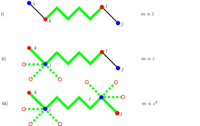
Figure 29: Sketch to visualize the three cases occurring in the double sum in equation (134). The distance between the red dots $k$ and $l$ defines the scaling of the expectation value in the double sum. The green zigzag lines indicates that the corresponding adjacent sites are connected via arbitrarily many bonds. By the green dashed lines with open red dots we indicate that there are multiple options for the sites $k$ or $l$.

Using the above multiplicities in combination with the scaling of the spin-spin correlations (131) we obtain that the pair correlations scale like

$$\langle\boldsymbol{V}^{\alpha}_{i}(t_{1})\boldsymbol{V}^{\beta}_{j}(t_{2})\rangle \propto\begin{cases}z^{-1}&\text{if $\norm{i-j}=1$,}\\ z^{-\norm{i-j}+1}&\text{if $\norm{i-j}>1$,}\\ \end{cases}$$ (135)

so that they are suppressed by at least the factor $z^{-1}$. Hence, no correlations between the local-environment fields need to be accounted for. By self-consistency, this extends to the second moments of the local mean-fields.

In a similar fashion, we show that the spin dynamics of $\vec{\boldsymbol{S}}_{i}$ is uncorrelated to its corresponding local-environment field $\vec{\boldsymbol{V}}_{i}$:

$$\langle\boldsymbol{S}^{\alpha}_{i}(t_{1})\boldsymbol{V}^{\beta}_{i}(t_{2})\rangle =\frac{1}{\sqrt{z}}\sum_{\gamma}J^{\beta\gamma}\overbrace{\sum_{k,\langle k,i\rangle}}^{\propto z}\underbrace{\langle\boldsymbol{S}^{\alpha}_{i}(t_{1})\boldsymbol{S}^{\gamma}_{k}(t_{2})\rangle}_{\propto z^{-1}}$$ (136a)

$$\propto z^{-\frac{1}{2}},$$ (136b)

as well as to any other local-environment field $\vec{\boldsymbol{V}}_{j}$ ($j\neq i$):

$$\langle\boldsymbol{S}^{\alpha}_{i}(t_{1})\boldsymbol{V}^{\beta}_{j}(t_{2})\rangle =\frac{1}{\sqrt{z}}\sum_{\gamma}J^{\beta\gamma}\sum_{k,\langle k,j\rangle}\langle\boldsymbol{S}^{\alpha}_{i}(t_{1})\boldsymbol{S}^{\gamma}_{k}(t_{2})\rangle$$ (137a)

$$\propto z^{-\norm{i-j}+\frac{1}{2}},$$ (137b)

which both tend to 0 for $z\to\infty$. For the last conclusion, one has to distinguish two cases again, see Fig. 30. First, site $i$ can be nearer to $j$ than to $k$. Second, site $i$ can be nearer to $k$ than to $j$. The latter case is dominant with a multiplicity of $m\propto 1$ and a scaling of $\propto z^{-\norm{j-1}+1}$. Together with the prefactor $1/\sqrt{z}$ this yields the provided scaling.

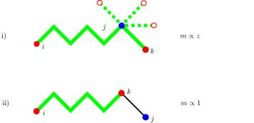
Figure 30: Sketch to visualize the two cases occurring in the site sum in equation (137). The distance between the red dots $k$ and $i$ defines the scaling of the expectation value on the right hand side. The green zigzag lines indicate that the corresponding adjacent sites are connected via arbitrarily many bonds. By the green dashed lines we indicate that there are multiple options for the site $k$.

Appendix B Error analyses

In this appendix, we discuss numerical errors and issues which arise in evaluating the mean-field moments. An assessment of the errors resulting from statistics, finite discretization, and convergence by iteration is provided. Subsequently, we explain how the numerical effort can be reduced by exploiting time translation invariance and we discuss the definiteness of the covariance matrices.

B.1 Statistical Error

By the self-consistent equations derived in Sect. II.3.2 the moments of the mean-fields are linked to spin expectation values which are calculated by path integrals averaged over the distribution of the mean-field time series $\vec{\mathcal{V}}$. Numerically, we estimate the path integrals using a Monte-Carlo method. The autocorrelations

$$g^{\alpha\beta}_{\vec{\mathcal{V}}}(t_{1},t_{2}):=\langle\boldsymbol{S}^{\alpha}(t_{1})\boldsymbol{S}^{\beta}(t_{2})\rangle^{\text{\tiny{(sts)}}}_{\vec{\mathcal{V}}}$$ (138)

are computed for $M$ time series $\vec{\mathcal{V}}$ and averaged

$$g_{M}^{\alpha\beta}(t_{1},t_{2}):=\frac{1}{M}\sum_{\vec{\mathcal{V}}}g^{\alpha\beta}_{\vec{\mathcal{V}}}(t_{1},t_{2})$$ (139)

which converges to $g^{\alpha\beta}(t_{1},t_{2})$ for $M\to\infty$. Since the time series are drawn independent of each other the variance of $g_{M}^{\alpha\beta}(t_{1},t_{2})$ is given by the variance of a single time series divided by $M$

$$\sigma^{2}\left(g^{\alpha\beta}_{M}(t_{1},t_{2})\right)=\frac{1}{M}\sigma^{2}\left(g_{\vec{\mathcal{V}}}^{\alpha\beta}(t_{1},t_{2})\right),$$ (140)

where $\sigma^{2}(\dots)$ denotes the variance of the quantity in the bracket.

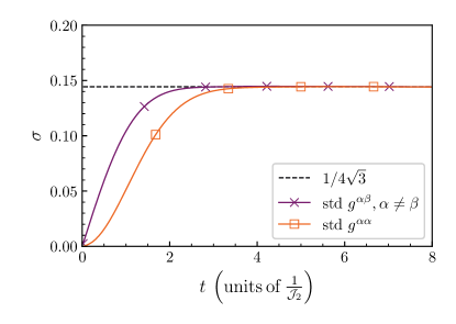
Figure 31: Numerical result for the standard deviations $\sigma\left(g_{\vec{\mathcal{V}}}^{\alpha\beta}(t,0)\right)$ as function of $t$ for the isotropic Heisenberg model without any magnetic field. For $t=0$, the autocorrelations are fixed and hence their standard deviation vanishes. For large $t$ it converges apparently to $1/4\sqrt{3}$, indicated by the dashed line.

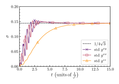
Figure 32: Same as Fig. 31 for the dipole model in the laboratory frame with $\vartheta=0$ at $\widetilde{B}=5.0$.

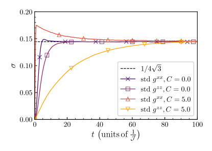
Figure 33: Same as Fig. 31 for the dipole model in the rotating frame in RWA and various noise strengths.

The standard deviation $\sigma$ of a single time series depends on many parameters and cannot be calculated analytically in a simple way. But it is clear that its value is bounded by the maximum value of the autocorrelations, i.e., by $\tfrac{1}{4}$. Figs. 31, 32, and 33 show generic time dependencies of $\sigma$ computed for different physical situations. Interestingly, we find that all of them converge to the value $1/(4\sqrt{3})$ for $t\to\infty$. The rapidity of this convergence depends on the actual decay of the corresponding autocorrelation. This behavior can be understood by the following argument. The autocorrelations vanish for large $t$. Hence, the variance equals the quadratic mean

$$\lim_{t\to\infty}\sigma^{2}\left(g^{\alpha\beta}(t,0)\right)=\lim_{t\to\infty}\overline{\bigl{(}(g^{\alpha\beta}(t,0)\bigr{)}^{2}}.$$ (141)

In a next step, we consider the vector-valued signal

$$\vec{g}^{\,\beta}_{\vec{\mathcal{V}}}(t,0) :=\langle\boldsymbol{U}^{\dagger}(t,0)\vec{\boldsymbol{S}}(0)\boldsymbol{U}(t,0)\boldsymbol{S}^{\beta}(0)\rangle^{\text{\tiny{(sts)}}}_{\vec{\mathcal{V}}}$$ (142a)

$$=\left\langle\left(\underline{\underline{R}}_{\vec{\mathcal{V}}}(t,0)\vec{\boldsymbol{S}}(0)\right)\boldsymbol{S}^{\beta}(0)\right\rangle^{\text{\tiny{(sts)}}}_{\phantom{\vec{V}}}$$ (142b)

$$=\frac{1}{4}\underline{\underline{R}}_{\vec{\mathcal{V}}}(t,0)\vec{\mathrm{e}}_{\beta},$$ (142c)

where $\underline{\underline{R}}_{\vec{\mathcal{V}}}(t,0)$ denotes the orthogonal rotation matrix which describes the rotation of the initial spin vector due to its temporal evolution subjected to the fluctuating time series $\vec{V}(t)$. Obviously, the square of $\vec{g}^{\,\beta}_{\vec{\mathcal{V}}}(t,0)$ is constant

$$\left(\vec{g}^{\beta}(t,0)\right)^{2}=\frac{1}{16}$$ (143)

before and thus also after averaging.

Next, it is plausible and in accord with all previous results that the decoherence is sufficiently strong to have the spin vector $\underline{\underline{R}}_{\vec{\mathcal{V}}}(t,0)\vec{\boldsymbol{S}}(0)$ lose all information about its initial direction. If it points in $z$ direction at $t=0$ it will point into any direction of the unit sphere after sufficiently long time. Therefore, each component $\alpha$ of the rotated spin vector has the same variance for $t\to\infty$ and contributes equally to the squared vector in (143). This allows us to conclude

$$\lim_{t\to\infty}\sigma\left(g^{\alpha\beta}(t,0)\right) =\lim_{t\to\infty}\sqrt{\overline{\left(\vec{g}^{\beta}(t,0)\right)^{2}}/3} =\frac{1}{4\sqrt{3}}$$ (144)

in perfect agreement with the numerical findings. This enables us to derive the reliable estimate

$$\sigma\left(g_{M}^{\alpha\beta}(t_{1},t_{2})\right)\approx\frac{1}{4\sqrt{3M}}.$$ (145)

for the statistical error from averaging over $M$ times series. It becomes even exact for $t\to\infty$.

B.2 Discretization Error

The goal of this appendix is to estimate the error resulting from the discretization of time, i.e., the error resulting from working with a finite time step $\delta t>0$ instead of taking $\delta t\to 0$. Certainly, this error will depend on details of the model. We discuss it for both the isotropic Heisenberg model and the dipole model without and with RWA.

We consider the discretization error of the diagonal autocorrelations $\alpha=\beta$ up to some maximum time $t_{\text{max}}$ which we determine such that

$$\lvert g^{\alpha\alpha}(t_{\text{max}})\rvert\approx\frac{1}{100}$$ (146)

holds, i.e., the autocorrelation has decreased to $1/25$ of its initial value. For simplicity, we focus on the autocorrelation that decays slowest in each physical scenario, since it is most susceptible to the discretization error which accumulates in the course of its temporal evolution. Mostly this is the longitudinal autocorrelation.

To be specific, we compute $g^{\alpha\alpha}(t)$ on the time interval $t\in[0,t_{\text{max}}]$ for various step widths

$$\delta t(\nu) =\delta t(0)2^{-\nu}, \nu \in[0,1,2,...,\nu_{\text{max}}].$$ (147)

The results for $g^{\alpha\alpha}(t)$ for $\nu<\nu_{\text{max}}$ are compared to the ‘best’ solution for $\nu_{\text{max}}$, i.e., the solution from the finest discretization which is used as reference. We define the discretization error

$$\overline{\Delta q}(\nu) =\sum_{l=0}^{L(\nu)}\frac{\lvert g^{\alpha\alpha}_{\nu_{\text{max}}}(l\delta t(\nu))-g^{\alpha\alpha}_{\nu}(l\delta t(\nu))\rvert}{L(\nu)+1}$$ (148)

where $L(\nu)=t_{\text{max}}/\delta t(\nu)$ is the number of time steps. We stress that the input data for $\overline{\Delta q}(\nu)$ are not exact, but subjected also to the statistical error discussed in the previous section.

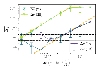
Figure 34: Numerical analysis of the time discretization error for the isotropic model. Data are shown for zero magnetic field (1) and for finite magnetic field $\gamma_{\text{s}}B=5.0\mathcal{J}_{2}$ (2) and, furthermore, for $M=$4\text{\times}{10}^{5}$$ (A) and for $M=$6.4\text{\times}{10}^{6}$$ (B) time series, respectively. The dashed line (A) and the dashed-dotted line (B) represent the statistical errors $\sigma$ for the corresponding $M$. The thin orange lines follow $\delta t^{2}$ and are given for comparison.

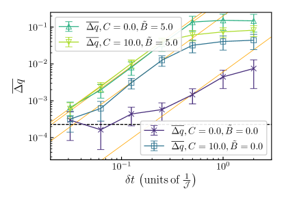
Figure 35: Numerical analysis of the time discretization error for the lab-frame dipole model with $\vartheta=0$ for various magnetic fields $\tilde{B}$ and noise widths $C$. The dashed line corresponds to the statistical error $\sigma$ for the sample size $M=$4\text{\times}{10}^{5}$$. The thin orange lines follow $\delta t^{2}$ and are given for comparison.

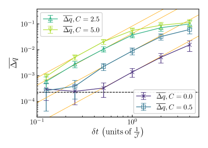
Figure 36: Numerical analysis of the time discretization error for the RWA dipole model for various noise widths $C$. The dashed line corresponds to the statistical error $\sigma$ for the sample size $M=$4\text{\times}{10}^{5}$$. The thin orange lines follow $\delta t^{2}$ and are given for comparison.

Figs. 34, 35, and 36 show the results for the three different models investigated in the main text. The qualitative behavior is very similar. For small values of $\delta t$ the deviation $\overline{\Delta q}$ is clearly dominated by the statistical error. Hence the curves level off displaying roughly plateaus with some fluctuations. For large values of $\delta t$ the curves also level off displaying a plateau. This stems from errors so large that the deviations are of order $2/4$ because the fluctuating diagonal autocorrelations $g^{\alpha\alpha}$ are bounded by $1/4$.

Thus, the relevant regime is at intermediate time steps between these two plateaus. Here the effect of the discretization can be discerned. The double logarithmic plots are consistent with the conclusion $\overline{\Delta q}\propto\delta t^{2}$ as can be read off by comparing to the straight lines resulting from the quadratic power law. This can be easily understood by the approximation we have to use for the unitary time evolution operators which propagate the system from $t$ to $t+\delta t$. The employed second-order CFET and the trapezoidal rule entail a discretization error scaling like $\delta t^{3}$. But since this error accumulates over time one has to multiply this scaling by the number of step from $t=0$ to $t=t_{\text{max}}$ so that we obtain

$$\overline{\Delta q}\propto L\delta t^{3}\propto\delta t^{2}.$$ (149)

This explains the observed quadratic scaling of the discretization error with the time step size $\delta t$.

Aside from the above discussed scaling further conclusions on the influence of the discretization can be drawn. Inspecting Figs. 34 and 35 shows that a finite magnetic field increases $\overline{\Delta q}$. The reason is that the Larmor precessions need to be resolved. If the step size $\delta t$ is too long, approaching the Larmor period, sizable discretization errors occur. As a rule of thumb, $\delta t$ should be at maximum a tenth of the Larmor precession period

$$T=\frac{2\pi}{\gamma_{\text{s}}B}.$$ (150)

Since the time discretization error accumulates over time longer lasting correlations imply larger discretization errors. This can be seen for instance in Fig. 36 where the dipole model is studied in RWA. The error $\overline{\Delta q}$ increases with the noise strength because the decay of the longitudinal autocorrelation is slowed down upon increasing $C$. Finally, we point out that a small discretization error is desirable. But in view of the efficiency of the total algorithm it does not pay to reduce the discretization error below the statistical error. Hence, the parameters should be set such that $\overline{\Delta q}\approx\sigma(g)$ holds.

B.3 Termination condition for the iteration

We determine the solution of the self-consistency conditions iteratively. If the algorithm is stable, the autocorrelation functions $g^{\alpha\beta}_{(i)}(t)$ of the iteration $i$ converge to the exact results for $i\to\infty$. In practice, it is necessary to define a termination condition to decide when the iterations can be stopped. For this we use

$$\Delta I^{\alpha\beta}\left(i\right)=\frac{1}{L+1}\sum_{l=0}^{L}\lvert g^{\alpha\beta}_{(i)}(t_{l})-g^{\alpha\beta}_{(i-1)}(t_{l})\rvert.$$ (151)

This quantity measures the difference between the results of iteration $j+1$ and $j$, where $j\geq 1$ . The execution of the code is stopped if $\Delta I^{\alpha\beta}\left(i\right)$ falls below a certain threshold. Since the iteration error itself is limited by the statistical accuracy this threshold cannot be chosen smaller than the statistical error. It needs to be set above the statistical standard deviation to achieve reliable termination. In our numerics, it turned out that

$$\Delta I_{\text{threshold}}=2\sigma\left(g_{M}^{\alpha\beta}(t_{1},t_{2})\right)=\frac{1}{2\sqrt{3M}}$$ (152)

is a reasonable choice. It avoids unnecessary iterations while it is strict enough to yield sufficient convergence.

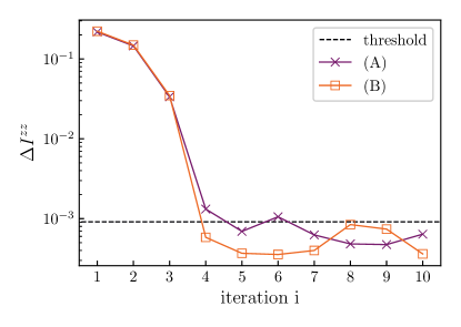
Figure 37: Iteration error $4\Delta I^{zz}$ as function of the iteration number $i$. Case (A) starts from an exponential initial diagonal autocorrelation and case (B) from a Gaussian initial diagonal autocorrelation. The error threshold (152) is displayed as horizontal dashed line for $M=$1\text{\times}{10}^{5}$$ time series. The termination condition is fulfilled at $i=5$ for case (A) and at $i=4$ for case (B).

Figure 37 depicts the iteration error of $g^{zz}$ for the isotropic Heisenberg model without magnetic field. The iterations started from two different initial diagonal autocorrelations $g^{\alpha\alpha}$ while the cross autocorrelations $g^{\alpha\beta}$ with $\alpha\neq\beta$ are set to zero. The iteration error decreases very fast in the beginning. At about the fourth iteration it reaches the magnitude of the threshold. Beyond the fourth iteration, statistical fluctuations stemming from the averaging over $M$ time series occur and dominate the iteration error $\Delta I^{xx}$. For optimum computational efficiency, the code should terminate before the statistical fluctuations take over.

We emphasize that the “converged” results obtained in this way are independent of the initially chosen autocorrelations. The deviation between the iterated results from the exponential and the Gaussian initial autocorrelation is of the same magnitude as the error threshold (152). For this reason, we consider the chosen iterative algorithm robust enough to determine physically meaningful solutions.

B.4 Time-Translation Invariance

For both the isotropic and the dipolar spin systems we considered a time-independent Hamiltonian so that the systems are invariant under time translation

$$\boldsymbol{U}(t_{2},t_{1})=\mathrm{e}^{-\texttt{i}\boldsymbol{H}\left(t_{2}-t_{1}\right)}=\boldsymbol{U}(t_{2}-t_{1},0)$$ (153)

and so are all two-time spin autocorrelations

$$\langle\boldsymbol{S}^{\alpha}(t_{1})\boldsymbol{S}^{\beta}(t_{2})\rangle=\langle\boldsymbol{S}^{\alpha}(t_{1}-t_{2})\boldsymbol{S}^{\beta}(0)\rangle.$$ (154)

Applying spinDMFT, the situation is slightly more complicated. The autocorrelations with respect to a single time series $\vec{\mathcal{V}}_{i}$ are not time-translation invariant because the mean-field is dynamic, i.e., it depends on time. But the physically meaningful expectation values are obtained by averaging over the distribution of possible mean-fields. In the path integral the mean-field $\vec{\mathcal{V}}_{i}$ can be shifted in time so that the time evolution operators and the distribution functional $p[\vec{\mathcal{V}}_{i}]$ are shifted. Time-translation invariance is ensured if and only if the distribution remains unchanged by this shift. Specifically, this is equivalent to the condition

$$\overline{V^{\alpha}(t_{1})V^{\beta}(t_{2})}=\overline{V^{\alpha}(t_{1}-t_{2})V^{\beta}(0)},$$ (155)

for the second moments of the mean-fields, i.e., they are time-translation invariant themselves. As stated in the main text, the time invariance of the moments and hence of the distribution implies time translation invariance of the spin-spin autocorrelations. So time-translational self-consistent solutions are possible, but it cannot be excluded that solutions exist which are not time-translationally invariant. Here, we do not consider them because they cannot occur in a quantum system at infinite temperature although time-crystalline behavior cannot be excluded generally for specific situations.

In practice, the averaging based on Monte-Carlo sampling allows for small unphysical violations of time translational invariance due to the finite statistical error: the self-consistently computed moments and autocorrelations may not be exactly time-translation invariant, even though the initially inserted moments have this property. To avoid violations of time translational invariance, we enforce it in each iteration step. A simple implementation consists in setting

$$t_{1} =\Delta t, t_{2} =0, \text{for}\quad t_{1} >t_{2},$$ (156a)

$$t_{2} =\Delta t, t_{1} =0, \text{for}\quad t_{2} >t_{1},$$ (156b)

where $\Delta t=|t_{1}-t_{2}|$, instead of considering all pairs of times $t_{1},t_{2}$.

The reduced set of data together with the assumption of time translation invariance provides all required information. Due to the time-translational invariance the covariance matrix has constant matrix elements on all diagonals

$$\underline{\underline{M}}^{\alpha\beta} =\begin{pmatrix}a&b&c&\\ \tilde{b}&a&b&\ddots\\ \tilde{c}&\tilde{b}&a&\ddots\\ &\ddots&\ddots&\ddots\\ \end{pmatrix},$$ (157)

where

$$a =\overline{V^{\alpha}(0)V^{\beta}(0)},$$ (158a)

$$b =\overline{V^{\alpha}(0)V^{\beta}(\delta t)}, \tilde{b} =\overline{V^{\alpha}(\delta t)V^{\beta}(0)},$$ (158b)

$$c =\overline{V^{\alpha}(0)V^{\beta}(2\delta t)}, \tilde{c} =\overline{V^{\alpha}(2\delta t)V^{\beta}(0)}.$$ (158c)

This procedure has two advantages: (i) time-translation invariance is built-in by construction; (ii) the autocorrelations need only be computed at the time differences $\Delta t$. Hence, the effort of steps 4) and 5) of the numerical procedure is reduced from $\mathcal{O}(L^{2})$ to $\mathcal{O}(L)$ where $L$ is the number of time steps.

B.5 Definiteness of the Covariance Matrix

In the self-consistency conditions the two-time correlations are taken as matrix elements of a covariance matrix. The physical justification is given in Sect. II. In addition, we discuss whether this identification is mathematically possible. To this end, the quantum correlations must provide (i) real symmetric matrix elements and the resulting matrix must be (ii) positive semi-definite.

In Sect. II.4 we already showed property (i) at infinite temperature. Property (ii) is equivalent to

$$\sum_{\alpha\beta}\sum_{t,t^{\prime}\in I}\langle\boldsymbol{V}_{i}^{\alpha}(t)\boldsymbol{V}_{i}^{\beta}(t^{\prime})\rangle\,\lambda^{{\alpha}}_{t}\lambda^{{\beta}}_{t^{\prime}}\geq 0,$$ (159)

for arbitrary real coefficients $\lambda_{t}^{{\alpha}}$ and $t\in I$ where $I$ is an arbitrary set of time instants. By shifting the sums into the expectation value we find

$$\Bigl{\langle}\Bigl{(}\underbrace{\sum_{\alpha}\sum_{t\in I}\boldsymbol{V}_{i}^{\alpha}(t)\lambda^{{\alpha}}_{t}}_{:=\boldsymbol{B}}\Bigr{)}^{2}\Bigr{\rangle}\geq 0.$$ (160)

Since $\boldsymbol{B}$ is a Hermitian operator, its square is a non-negative operator and thus any of its expectation values are non-negative. This proves the required positive semi-definiteness and applies to the expectation values of the path integral (15) and extends to the averages (139).

There is, however, a subtlety in the implementation described in the previous section. We guaranteed time translation invariance by using

$$\frac{1}{M}\sum_{\vec{\mathcal{V}}}g^{\alpha\beta}_{\vec{\mathcal{V}}}(t_{1},t_{2})\approx\frac{1}{M}\sum_{\vec{\mathcal{V}}}g^{\alpha\beta}_{\vec{\mathcal{V}}}(\Delta t,0).$$ (161)

For $M=\infty$ this is relation holds exactly true. But the statistical fluctuations at finite $M$ imply that the covariance matrix computed by Eq. (157) need not be non-negative. If we refrained from setting all matrix elements on a diagonal constant, but used the two-time autocorrelations, $\underline{\underline{L}}$ would be non-negative. Enforcing time translation invariance breaks the positive semi-definiteness to the extent of the statistical standard deviation. Since we keep this deviation low the computed covariance matrices are very close to being non-negative. Due to the Monte Carlo approach to the averaging all numerical results are subjected to the statistical error so that the statistical inaccuracies of the approximate covariance matrix are no source of additional deviations.

Practically, we diagonalize the approximate covariance matrix and set the eigenvalues which are negative to zero for the next iteration step. We stress that the modulus of these negative eigenvalues is of the order of the statistical error, i.e., small in a systematically controlled way. Therefore, the employed procedure provides consistent physical solutions for the dynamic autocorrelations within the discussed errors.