Rectifying the Shortcut Learning of Background for Few-Shot Learning

Abstract

The category gap between training and evaluation has been characterised as one of the main obstacles to the success of Few-Shot Learning (FSL). In this paper, we for the first time empirically identify image background, common in realistic images, as a shortcut knowledge helpful for in-class classification but ungeneralizable beyond training categories in FSL. A novel framework, COSOC, is designed to tackle this problem by extracting foreground objects in images at both training and evaluation without any extra supervision. Extensive experiments carried on inductive FSL tasks demonstrate the effectiveness of our approaches.

1 Introduction

Through observing a few samples at a glance, humans can accurately identify brand-new objects. This advantage comes from years of experiences accumulated by the human vision system. Inspired by such learning capabilities, Few-Shot Learning (FSL) is developed to tackle the problem of learning from limited data Alexander et al. (1995, 1995). At training, FSL models absorb knowledge from a large-scale dataset; later at evaluation, the learned knowledge is leveraged to solve a series of downstream classification tasks, each of which contains very few support (training) images from brand-new categories.

The category gap between training and evaluation has been considered as one of the core issues in FSL Alexander et al. (1995). Intuitively, the prior knowledge of old categories learned at training may not be applicable to novel ones. Alexander et al. (1995) consider solving this problem from a causal perspective. Their backdoor adjustment method, however, adjusts the prior knowledge in a black-box manner and cannot tell which specific prior knowledge is harmful and should be suppressed.

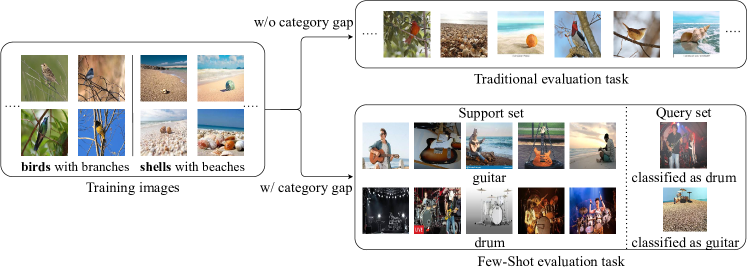
Figure 1: An illustrative example that demonstrates why background information is useful for regular classification but harmful for few-shot learning.

In this paper, we, for the first time, identify image background as one specific harmful source knowledge for FSL. Empirical studies in Alexander et al. (1995) suggest that there exists spurious correlations between background and category of images (e.g., birds usually stand on branches, and shells often lie on the beaches; see Fig. 1), which serves as a shortcut knowledge for modern CNN-based vision systems to learn. It is further revealed that background knowledge has positive impact on the performance of in-class classification tasks. As illustrated in the simple example of Fig. 1, images from the same category are more likely to share similar background, making it possible for background knowledge to generalize from training to testing in common classification tasks. For FSL, however, the category gap produces brand-new foreground, background and their combinations at evaluation. The correlations learned at training thus may not be able to generalize and would probably mislead the predictions. We take empirical investigations on the role of image foreground and background in FSL, revealing how image background drastically affects the learning and evaluation of FSL in a negative way.

Since the background is harmful, it would be good if we could force the model to concentrate on foreground objects at both training and evaluation, but this is not easy since we do not have any prior knowledge of the entity and position of the foreground objects in images. When humans are going to recognize foreground objects of images from the same class, they usually look for a shared local pattern that appears in the majority of images, and recognize patches with this pattern as foreground. This inspires us to design a novel framework, COSOC, to extract foreground of images for both training and evaluation of FSL by seeking shared patterns among images. The approach does not depend on any additional fine-grained supervisions such as bounding boxes or pixel-level labelings.

The procedure of foreground extraction of images in the training set is implemented before training. The corresponding algorithm, named Clustering-based Object Seeker (COS), first pre-trains a feature extractor on the training set using contrative learning, which has an outstanding performance, shown empirically in a later section, on the task of discriminating between ground-truth foreground objects. The feature extractor then maps random crops of images—candidates of foreground objects—into a well-shaped feature space. This is followed by runing a clustering algorithm on all of the features of the same class, imitating the procedure of seeking shared local patterns inspired by human behavior. Each cropped patch is then assigned a foreground score according to its distance to the nearest cluster centroid, for determining a sampling probability of that patch in the later formal training of FSL models. For evaluation, we develop Shared Object Concentrator (SOC), an algorithm that applies iterative feature matching within the support set, looking for one crop per image at one time that is most likely to be foreground. The sorted averaging features of obtained crops are further leveraged to match crops of query images so that foreground crops have higher matching scores. A weighted sum of matching scores are finally calculated as classification logits of each query sample. Compared to other potential foreground extracting algorithms such as saliency-based methods, our COS and SOC algorithms have additional capability of capturing shared, inter-image information, performing better in complicated, multi-object scenery. Our methods also have flexibility of dynamically assigning beliefs (probabilities) to all candidate foreground objects, relieving the risk of overconfidence.

Our contributions can be summarized as follows. i) By conducting empirical studies on the role of image foreground and background in FSL, we reveal that image background serves as a source of shortcut knowledge which harms the evaluation performance. ii) To solve this problem, we propose COSOC, a framework combining COS and SOC, which can draw the model’s attention to image foreground at both training and evaluation. iii) Extensive experiments for non-transductive FSL tasks demonstrate the effectiveness of our method.

2 Related Works

Few-shot Image Classification. Plenty of previous work tackled few-shot learning in meta-learning framework Alexander et al. (1995, 1995), where a model learns experience about how to solve few-shot learning tasks by tackling pseudo few-shot classification tasks constructed from the training set. Existing methods that ultilize meta-learning can be generally divided into three groups: (1) Optimization-based methods learn the experience of how to optimize the model given few training samples. This kind of methods either meta-learn a good model initialization point Alexander et al. (1995, 1995, 1995, 1995, 1995) or the whole optimization process Alexander et al. (1995, 1995, 1995, 1995) or both Alexander et al. (1995, 1995). (2) Hallucination-based methods Alexander et al. (1995, 1995, 1995, 1995, 1995, 1995, 1995, 1995) learn to augment similar support samples in few-shot tasks, thus can greatly alleviate the low-shot problem. (3) Metric-based methods Alexander et al. (1995, 1995, 1995, 1995, 1995) learn to map images into a metric feature space and classify query images by computing feature distances to support images. Among them, several recent works Alexander et al. (1995, 1995, 1995, 1995) intended to seek correspondence between images either by attention or meta-filter, in order to obtain a more reasonable similarity measure. Our SOC algorithm in one-shot setting is in spirit similar to these methods, in that we both apply pair-wise feature alignment between support and query images, implicitly removing backgrounds that are more likely to be dissimilar across images. SOC differs in multi-shot setting, where potentially useful shared inter-image information in support set exists and can be captured by our SOC algorithm.

The Influence of Background. A body of prior work studied the impact of image background on learning-based vision systems from different perspectives. Alexander et al. (1995) showed initial evidence of the existence of background correlations and how it influences the predictions of vision models. Alexander et al. (1995, 1995) analyzed background dependence for object detection. Another relevant work Alexander et al. (1995) utilized camera traps for investigating how performance drops when adapting classifiers to unseen cameras with novel backgrounds. They explore the effect of class-independent background (i.e., background changes from training to testing while categories remain the same) on classification performance. Although the problem is also concerned with image background, no shortcut learning of background exists under this setting. This is because under each training camera trap, the classifier must distinguish different categories with background fixed, causing the background knowledge being not useful for predictions of training images. Instead, the learning signal during training pushes the classifier towards ignoring each specific background. The difficulties under this setting lie in the domain shift challenge—the classifier is confident to handle previously existing backgrounds, but lost in novel backgrounds. More recently, Alexander et al. (1995) systematically explore the role of image background in modern deep-learning-based vision systems through well-designed experiments. The results give clear evidence on the existence of background correlations and identify it as a positive shortcut knowledge for models to learn. Our results, on the contrary, identify background correlations as a negative knowledge in the context of few-shot learning.

Contrastive Learning. Recent success on contrastive learning of visual representations has greatly promoted the development of unsupervised learning Alexander et al. (1995, 1995, 1995, 1995). The promising performance of contrastive learning relies on the instance-level discrimination loss which maximizes agreement between transformed views of the same image and minimizes agreement between transformed views of different images. Recently there have been some attempts Alexander et al. (1995, 1995, 1995, 1995, 1995, 1995) at integrating contrastive learning into the framework of FSL. Although achieving good results, these work struggle to have an in-depth understanding of why contrastive learning has positive effects on FSL. Our work takes a step forward, revealing the advantages of contrastive learning over supervised FSL models in identifying core objects of images.

3 Empirical Investigation

Problem Definition. Few-shot learning consists of a training set $\mathcal{D}_{B}$ and an evaluation set $\mathcal{D}_{v}$ which share no overlapping classes. $\mathcal{D}_{B}$ contains a large amount of labeled data and is usually used at first to train a backbone network $f_{\theta}(\cdot)$. After training, a set of $N$-way $K$-shot classification tasks $\mathcal{T}=\{(\mathcal{S}_{\tau},\mathcal{Q}_{\tau})\}_{\tau=1}^{N_{\mathcal{T}}}$ are constructed, each by first sampling $N$ classes in $D_{v}$ and then sampling $K$ and $M$ images from each class to constitute $\mathcal{S}_{\tau}$ and $\mathcal{Q}_{\tau}$, respectively. In each task $\tau$, given the learned backbone $f_{\theta}(\cdot)$ and a small support set $\mathcal{S}_{\tau}=\{(x_{k,n}^{\tau},y_{k,n}^{\tau})\}_{k,n=1}^{K,N}$ consisting of $K$ images $x_{k,n}^{\tau}$ and corresponding labels $y_{k,n}^{\tau}$ from each of $N$ classes, a few-shot classification algorithm is designed to classify $MN$ images from the query set $\mathcal{Q}_{\tau}=\{(x_{mn}^{\tau})\}_{m,n=1}^{M,N}$.

Preparation. To investigate the role of background and foreground in FSL, we need ground-truth image foreground for comparison. However, it is time-consuming to label the whole dataset. Thus we select only a subset $\mathcal{D}_{\mathrm{new}}=(\mathcal{D}_{B},\mathcal{D}_{v})$ of miniImageNet Alexander et al. (1995) and crop each image manually according to the largest rectangular bounding box that contains the foreground object. We denote the uncropped version of the subset as $(\mathcal{D}_{B}$-$\mathrm{Ori},\mathcal{D}_{v}$-$\mathrm{Ori})$, and the cropped foreground version as $(\mathcal{D}_{B}$-$\mathrm{FG},\mathcal{D}_{v}$-$\mathrm{FG})$. Two well-known FSL baselines are selected in our empirical studies: Cosine Classifier (CC) Alexander et al. (1995) and Prototypical Networks (PN) Alexander et al. (1995). See Appendix A for details of constructing $\mathcal{D}_{\mathrm{new}}$ and a formal introdcution of CC and PN.

3.1 The Role of Foreground and Background in Few-Shot Image Classification

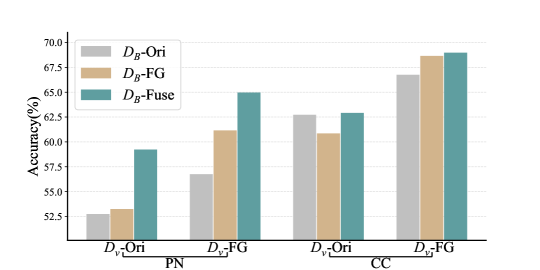
Figure 2: 5-way 5-shot FSL performance on different variants of training and evaluation datasets detailed in Sec. 3. (a) Empirical exploration of image foreground and background in FSL using two models: PN and CC. (b) Comparison between CC and Exemplar trained on the full training set of miniImageNet and evaluated on $\mathcal{D}_{v}$-$\mathrm{Ori}$ and $\mathcal{D}_{v}$-$\mathrm{FG}$.

Fig. 2 shows the average of 5-way 5-shot classification accuracy obtained by training CC and PN on $\mathcal{D}_{B}$-$\mathrm{Ori}$ and $\mathcal{D}_{B}$-$\mathrm{FG}$, and evaluating on $\mathcal{D}_{v}$-$\mathrm{Ori}$ and $\mathcal{D}_{v}$-$\mathrm{FG}$, respectively. See Appendix F for additional 5-way 1-shot experiments.

Category gap disables generalization of background knowledge. It can be first noticed that, under any condition, the performance is consistently and significantly improved if background is removed at the evaluation stage (switch from $\mathcal{D}_{v}$-$\mathrm{Ori}$ to $\mathcal{D}_{v}$-$\mathrm{FG}$). The result implies that background at the evaluation stage in FSL is harmful. This is the opposite of that reported in Alexander et al. (1995) which shows background helps improve on the performance of traditional classification task, where no category gap exists between training and evaluation. Thus we can infer that the class/distribution gap in FSL disables generalization of background knowledge and degrades performance.

Removing background at training prevents shortcut learning. When only foreground is given at evaluation ($\mathcal{D}_{v}$-$\mathrm{FG}$), the models trained with only foreground ($\mathcal{D}_{B}$-$\mathrm{FG}$) perform much better than those trained with original images ($\mathcal{D}_{B}$-$\mathrm{Ori}$). This indicates that models trained with original images may not pay enough attention to the foreground object that really matters for classification. Background information at training serves as a shortcut for models to learn and cannot generalize to brand-new classes. In contrast, models trained with only foreground "learn to compare" different objects—a desirable ability for reliable generalization to downstream few-shot learning tasks with out-of-domain classes.

Training with background helps models to handle complex scenes. When evaluating on $\mathcal{D}_{v}$-$\mathrm{Ori}$, the models trained with original dataset $\mathcal{D}_{B}$-$\mathrm{Ori}$ are slightly better than those with foreground dataset $\mathcal{D}_{B}$-$\mathrm{FG}$. We attribute this to a sort of domain shift: models trained with $\mathcal{D}_{B}$-$\mathrm{FG}$ never meet images with complex background and do not know how to handle it. In Appendix D.1 we further verify the assertion by showing evaluation accuracy of each class under the above two training situations. Note that since we apply random crop augmentation at training, domain shift does not exist if the models are instead trained on $\mathcal{D}_{B}$-$\mathrm{Ori}$ and evaluated on $\mathcal{D}_{v}$-$\mathrm{FG}$.

Simple fusion sampling combines advantages of both sides. One may wish to cut off shortcut learning of background while maintaining adaptability of model to complex scenes. A simple solution may be fusion sampling: given an image as input, choose its foreground version with probability $p$, and its original version with probability $1-p$. We simply set $p$ equal to $0.5$. We denote the dataset using this sampling strategy as $\mathcal{D}_{B}$-$\mathrm{Fuse}$. As observed in Fig. 2, models trained this way indeed combine advantages of both sides: achieving relatively good performance on both $\mathcal{D}_{v}$-$\mathrm{Ori}$ and $\mathcal{D}_{v}$-$\mathrm{FG}$. In Appendix C, we compare the training curves of PN trained on three versions of datasets to further investigate the effectiveness of fusion sampling.

The above analysis provides new inspiration for how to improve FSL further: (1) Fusion sampling of foreground and original images could be applied to training. (2) Since background information disturbs evaluation, it is needed to focus on foreground objects or assign image patches, that are more likely to be foreground, a larger weight for classification. Therefore, a foreground object identification mechanism is required at both training (for fusion sampling) and evaluation.

3.2 Contrastive Learning is Good at Identifying Objects

In this subsection, we reveal the potential of contrastive learning in identifying foreground objects, which we will use later for foreground extraction. Given one transformed view of one image, contrastive learning tends to distinguish another transformed view of that same image from thousands of views of other images. A more detailed introduction of contrastive learning is given in Appendix B. The two augmented views of the same image always cover the same object, but probably with different parts, sizes and color. To discriminate two augmented patches from thousands of other image patches, the model has to learn to identify the key discriminative information of the object under varying environment. In this manner, semantic relations among crops of images are explicitly modeled, thereby clustering semantically similar contents automatically. The features of different images are pushed away, while those of similar objects in different images are pulled closer. Thus it is reasonable to speculate that contrastive learning may enable models with better identification of centered foreground object.

To verify this, we train CC and contrastive learning models on the whole training set of miniImageNet ($\mathcal{D}_{B}$-$\mathrm{Full}$) and compare their accuracy on $\mathcal{D}_{v}$-$\mathrm{Ori}$ and $\mathcal{D}_{v}$-$\mathrm{FG}$. The contrastive learning method we use is Exemplar Alexander et al. (1995), a modified version of MoCo Alexander et al. (1995). Fig 2 shows that, while the evaluation accuracy of Exemplar on $\mathcal{D}_{v}$-$\mathrm{Ori}$ is slightly worse than that of CC, Exemplar performs much better when only foreground of images are given at evaluation, affirming that contrastive learning indeed has a better discriminative ability of single centered object. In Appendix D.2, we provide a more in-depth analysis of why contrastive learning has such properties and infer that the shape bias and viewpoint invariance may play an important role.

4 Rectifying the Shortcut Learning of Background

Given the analysis in the previous section, we wish to focus more on image foreground both at training and evaluation. Inspired by how humans recognise foreground objects, we propose COSOC, a framework ultilizing contrastive learning to draw the model’s attention to the foreground objects of images.

4.1 Clustering-based Object Seeker (COS) with Fusion Sampling for Training

Since contrastive learning is good at discriminating foreground objects, we utilize it to extract foreground objects before training. The first step is to pre-train a backbone $f_{\theta}(\cdot)$ on the training set $\mathcal{D}_{B}$ using Exemplar Alexander et al. (1995). Then a clustering-based algorithm is used to extract "objects" identified by the pre-trained model. The basic idea is that features of foreground objects in images within one class extracted by contrastive learning models are similar, thereby can be identified via a clustering algorithm; see a simple example in Fig. 3. All images within the $i$-th class in $\mathcal{D}_{B}$ form a set $\{\mathbf{x}_{n}^{i}\}_{n=1}^{N}$. For clarity, we omit the class index $i$ in the following descriptions. The scheme of seeking foreground objects in one class is detailed as follows:

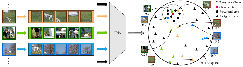
Figure 3: Simplified schematic illustration of COS algorithm. We show how we obtain foreground objects from three exemplified images. The value under each crop denotes its foreground score.

1) For each image $\mathbf{x}_{n}$, we randomly crop it $L$ times to obtain $L$ image patches $\{\mathbf{p}_{n,m}\}_{m=1}^{L}$. Each image patch $\mathbf{p}_{n,m}$ is then passed through the pre-trained model $f_{\theta}$ and we get a normalized feature vector $\mathbf{v}_{n,m}=\frac{f_{\theta}(\mathbf{p}_{n,m})}{||f_{\theta}(\mathbf{p}_{n,m})||_{2}}\in\mathbb{R}^{d}$.

2) We run a clustering algorithm $\mathcal{A}$ on all features vectors of the class and obtain $H$ clusters $\{\mathbf{z}_{j}\}_{j=1}^{H}=\mathcal{A}(\{\mathbf{v}_{n,m}\}_{n,m=1}^{N,L})$, where $\mathbf{z}_{j}$ is the feature centroid of the $j$-th cluster.

3) We say an image $\mathbf{x}_{n}\in\mathbf{z}_{j}$, if there exists $k\in[L]$ s.t. $\mathbf{v}_{n,k}\in\mathbf{z}_{j}$, where $[L]=\{1,2,\dots,L\}$. Let $l(\mathbf{z}_{j})=\frac{\#\{\mathbf{x}|\mathbf{x}\in\mathbf{z}_{j}\}}{N}$ be the proportion of images in the class that belong to $\mathbf{z}_{j}$. If $l(\mathbf{z}_{j})$ is small, then the cluster $\mathbf{z}_{j}$ is not representative for the whole class and is possibly background. Thus we remove all the clusters $\mathbf{z}$ with $l(\mathbf{z})<\gamma$, where $\gamma$ is a threshold that controls the generality of clusters. The remaining ${h}$ clusters $\{\mathbf{z}_{j}\}_{j=\alpha_{1}}^{\alpha_{h}}$ represent “objects” of the class that we are looking for.

4) The foreground score of image patch $p_{n,m}$ is defined as $s_{n,m}=1-\min_{j\in[h]}||\mathbf{v}_{n,m}-\mathbf{z}_{\alpha_{j}}||_{2}/\eta$, where $\eta=\max\limits_{n,m}\min\limits_{j\in[h_{c}]}||\mathbf{v}_{n,m}-\mathbf{z}_{\alpha_{j}}||_{2}$ is used to normalize the score into $[0,1]$. Then top-k scores of each image $\mathbf{x}_{n}$ are obtained as $\{s_{n,m}\}_{m=\beta_{1}}^{\beta_{k}}=\mathop{\mathrm{Topk}}\limits_{m\in[L]}(s_{n,m})$. The corresponding patches $\{\mathbf{p}_{n,m}\}_{m=\beta_{1}}^{\beta_{k}}$ are seen as possible crops of the foreground object in image $\mathbf{x}_{n}$, and the foreground scores $\{s_{n,m}\}_{m=\beta_{1}}^{\beta_{k}}$ as the confidence. We then use it as prior knowledge to rectify the shortcut learning of background for FSL models.

The training strategy resembles fusion sampling introduced before. For an image $\mathbf{x}_{n}$, the probability that we choose the original version is $1-\max\limits_{i\in{[k]}}s_{n,\beta_{i}}$, and the probability of choosing $\mathbf{p}_{n,\beta_{j}}$ from top-k patches is $(s_{n,\beta_{j}}/\sum_{i\in{[k]}}s_{n,\beta_{i}})\cdot\max\limits_{i\in{[k]}}s_{n,\beta_{i}}$. Then we adjust the chosen image patch and make sure that the least area proportion to the original image keeps as a constant. We use this strategy to train a backbone $f_{\theta}(\cdot)$ using a FSL algorithm.

4.2 Few-shot Evaluation with Shared Object Concentrator (SOC)

As discussed before, if the foreground crop of the image is used at evaluation, the performance of FSL model will be boosted by a large margin, serving as an upper bound of the model performance. To approach this upper bound, we propose SOC algorithm to capture foreground objects by seeking shared contents among support images of the same class and query images.

Figure 4: The overall pipeline of step 1 in SOC. Points in one color represent features of crops from one image. The red points are $\bm{\omega}_{1},\bm{\omega}_{2}$ and $\bm{\omega}_{3}$.

Step 1: Shared Content Searching within Each Class. For each image $\mathbf{x}_{k}$ within one class $c$ from support set $\mathcal{S}_{\tau}$, we randomly crop it $V$ times and obtain corresponding candidates $\{\mathbf{p}_{k,n}\}_{n=1,..,V}$. Each patch $\mathbf{p}_{k,n}$ is individually sent to the learned backbone $f_{\theta}$ to obtain a normalized feature vector $\mathbf{v}_{k,n}$. Thus we have totally $K\times V$ feature vectors within a class $c$. Our goal is to obtain a feature vector $\bm{\omega}_{1}$ that contains maximal shared information of all images in class $c$. Ideally, $\bm{\omega}_{1}$ represents the centroid of the most similar $K$ image patches, each from one image, which can be formulated as

$$\bm{\omega}_{1} =\frac{1}{K}\sum_{k=1}^{K}\mathbf{v}_{k,\lambda_{opt}(k)},$$ (1)

$$\lambda_{opt} =\mathop{\arg\max}\limits_{\lambda\in[K]^{[V]}}\sum_{1\leq i<j\leq K}\mathrm{cos}(\mathbf{v}_{i,\lambda(i)},\mathbf{v}_{j,\lambda(j)}),$$ (2)

where $\mathrm{cos}(\cdot,\cdot)$ denotes cosine similarity and $[K]^{[V]}$ denotes the set of functions that take $[K]$ as domain and $[V]$ as range. While $\lambda_{opt}$ can be obtained by enumerating all possible combinations of image patches, the computation complexity of this brute-force method is $\mathcal{O}(V^{K})$, which is computation prohibitive when $V$ or $K$ is large. Thus when the computation is not affordable, we turn to use a simplified method that leverages iterative optimization. Instead of seeking for the closest image patches, we directly optimize $\bm{\omega}_{1}$ so that the sum of minimum distance to patches of each image is minimized, i.e.,

$$\bm{\omega}_{1}=\mathop{\arg\max}\limits_{\bm{\omega}\in\mathcal{R}^{d}}\sum_{k=1}^{K}{\max_{n}[\cos(\bm{\omega},\mathbf{v}_{k,n})]},$$ (3)

which can be achieved by iterative optimization algorithms. We apply SGD in our experiments. After optimization, we remove the patch of each image that is most similar to $\bm{\omega}_{1}$, and obtain $K\times(V-1)$ feature vectors. Then we repeatedly implement the above optimization process until no features are left, as shown in Fig. 4. We eventually obtain $V$ sorted feature vectors $\{\bm{\omega}_{n}\}_{n=1}^{V}$, which we use to represent the class $c$. As for the case where shot $K=1$, there is no shared inter-image information inside class, so similar to the handling in PN and DeepEMD Alexander et al. (1995) , we just skip step 1 and use the original $V$ feature vectors.

Step 2: Feature Matching for Concentrating on Foreground Object of Query Images. Once the foreground class representations are identified, the next step is to use them to implicitly concentrate on foreground of query images by feature matching. For each image $\mathbf{x}$ in the query set $\mathcal{Q}_{\tau}$, we also randomly crop it for $V$ times and obtain $V$ candidate features $\{\bm{\mu}_{n}\}_{n=1}^{V}$. For each class $c$, we have $V$ sorted representative feature vectors $\{\bm{\omega}_{n}\}_{n=1}^{V}$ obtained in step 1. We then match the most similar patches between query features and class features, i.e.,

$$s_{1}=\max_{1\leq i,j\leq V}[\alpha^{j-1}\mathrm{cos}(\bm{\mu}_{i},\bm{\omega}_{j})],$$ (4)

where $\alpha\leq 1$ is an importance factor. Thus the weight $\alpha^{j-1}$ decreases exponentially in index $n-1$, indicating a decreased belief of each vector representing foreground. Similarly, the two matched features are removed and the above process repeats until no features left. Finally, the score of $\mathbf{x}$ w.r.t. class $c$ is obtained as a weighted sum of all similarities, i.e., $S_{c}=\sum_{n=1}^{V}\beta^{n-1}s_{n}$, where $\beta\leq 1$ is another importance factor controlling the belief of each crop being foreground objects. In this way, features matched earlier—thus more likely to be foreground—will have higher contributions to the score. The predicted class of $\mathbf{x}$ is the one with the highest score.

5 Experiments

5.1 Experiment Setup

Dataset. We adopt two benchmark datasets which are the most representative in few-shot learning. The first is miniImageNet Alexander et al. (1995), a small subset of ILSVRC-12 Alexander et al. (1995) that contains 600 images within each of the 100 categories. The categories are split into 64, 16, 20 classes for training, validation and evaluation, respectively. The second dataset, tieredImageNet Alexander et al. (1995), is a much larger subset of ILSVRC-12 and is more challenging. It is constructed by choosing 34 super-classes with 608 categories. The super-classes are split into 20, 6, 8 super-classes which ensures separation between training and evaluation categories. The final dataset contains 351, 97, 160 classes for training, validation and evaluation, respectively. On both datasets, the input image size is 84 × 84 for fair comparison.

Evaluation Protocols. We follow the 5-way 5-shot (1-shot) FSL evaluation setting. Specifically, 2000 tasks, each contains 15 testing images and 5 (1) training images per class, are randomly sampled from the evaluation set $\mathcal{D}_{v}$ and the average classification accuracy is computed. This is repeated 5 times and the mean of the average accuracy with 95% confidence intervals is reported.

Implementation Details. The backbone we use throughout the article is ResNet-12, which is widely used in few-shot learning. We use Pytorch Alexander et al. (1995) to implement all our experiments on two NVIDIA 1080Ti GPUs. We train the model using SGD with cosine learning rate schedule without restart to reduce the number of hyperparameters (Which epochs to decay the learning rate). The initial learning rate for training Exemplar is $0.1$, and for CC is $0.005$. The batch size for Exemplar, CC are 256 and 128, respectively. For miniImageNet, we train Exemplar for 150k iterations, and train CC for 6k iterations. For tieredImageNet, we train Exemplar for approximately 900k iterations, and train CC for 120k iterations. We choose k-means Alexander et al. (1995) as the clustering algorithm for COS. The threshold $\gamma$ is set to $0.5$, and top $3$ out of $30$ features are chosen per image at the training stage. At the evaluation stage, we crop each image $7$ times. The importance factors $\alpha$ and $\beta$ are both set to $0.8$.

5.2 Model Analysis

In this subsection, we show the effectiveness of each component of our method. Tab. 1 shows the ablation study conducted on miniImageNet.

On the effect of finetuning. Since a feature extractor is pre-trained using contrastive learning in COS, it may help accelerate convergence if we directly finetune from the pre-trained model instead of training from scratch. As shown in line 2-3 in Tab. 1, fintuning gives no improvement on the performance over training from scratch. Thus we adopt finetuning mainly for speeding up convergence (5$\times$ faster).

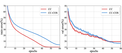
Figure 5: Comparison of training and validation curves between CC with and without COS.

Effectiveness of COS Algorithm. As observed in Tab. 1, When COS is applied on CC, the performance is improved on both versions of datasets. In Fig. 5, we show the curves of training and validation error of CC during training with and without COS. Both models are trained from scratch and validated on the full miniImageNet. We observe that CC sinks into overfitting: the training accuracy drops to zero, and validation accuracy stops improving before the end of the training. Meanwhile, the COS algorithm helps slow down convergence and prevent training accuracy from reaching zero. This makes validation accuracy comparable at first but higher at the end. Our COS algorithm weakens the “background shortcut” for learning, draws model’s attention on foreground objects, and improves upon generalization.

Table 1: Ablative study on miniImageNet. All models are trained on the full training set of miniImageNet. Since the aim of SOC algorithm is to find foreground objects, it is unnecessary to evaluate SOC on the foreground dataset $\mathcal{D}_{v}$-$\mathrm{FG}$. FT means finetuning from Exemplar used in COS.

CC	FT	COS	SOC	$\mathcal{D}_{v}$-$\mathrm{Ori}$		$\mathcal{D}_{v}$-$\mathrm{FG}$
				1-shot	5-shot	1-shot	5-shot
✓				62.67 $\pm$ 0.32	80.22 $\pm$ 0.24	66.69 $\pm$ 0.32	82.86 $\pm$ 0.19
✓		✓		64.76 $\pm$ 0.13	81.18 $\pm$ 0.21	71.13 $\pm$ 0.36	86.21 $\pm$ 0.15
✓	✓	✓		65.05 $\pm$ 0.06	81.16 $\pm$ 0.17	71.36 $\pm$ 0.30	86.20 $\pm$ 0.14
✓	✓		✓	64.41 $\pm$ 0.22	81.54 $\pm$ 0.28	-	-
✓	✓	✓	✓	69.29 $\pm$ 0.12	84.94 $\pm$ 0.28	-	-

Table 2: Comparisons with baselines of foreground extractors using saliency detection algorithms on miniImageNet. For fair comparison, all models in the right column at evaluation use multi-cropping. GT means evaluating with ground truth foreground.

Used for training			Used for evaluation
Method	1-shot	5-shot	Method	1-shot	5-shot
CC	62.67 $\pm$ 0.32	80.22 $\pm$ 0.24	COS	67.23 $\pm$ 0.35	82.79 $\pm$ 0.31
CC+RBD	63.24 $\pm$ 0.41	80.45 $\pm$ 0.37	COS+RBD	67.03 $\pm$ 0.52	82.57 $\pm$ 0.27
CC+MBD	61.50 $\pm$ 0.31	79.12 $\pm$ 0.32	COS+MBD	62.98 $\pm$ 0.45	79.56 $\pm$ 0.38
CC+FT	62.71 $\pm$ 0.11	80.06 $\pm$ 0.08	COS+FT	64.74 $\pm$ 0.28	80.74 $\pm$ 0.13
CC+COS	64.76 $\pm$ 0.13	81.18 $\pm$ 0.21	COSOC	69.28 $\pm$ 0.49	85.16 $\pm$ 0.42
-	-	-	COS+GT	72.71 $\pm$ 0.57	87.43 $\pm$ 0.36

Effectiveness of SOC Algorithm. The result in Tab. 1 shows that the SOC algorithm is the key to maximally exploit the potential of good object-discrimination ability. The performance even approaches the upper bound performance obtained by evaluating the model on the ground-truth foreground $\mathcal{D}_{v}$-$\mathrm{FG}$. One potential unfairness in our SOC algorithm may lie in the use of multi-cropping, which could possibly lead to performance improvement for other approaches as well. We ablate this concern in Appendix G, as well as in the comparisons to other methods in the later subsections.

Note that if we apply only the SOC algorithm on CC, the performance degrades. This indicates that COS and SOC are both necessary: COS provides the discrimination ability of foreground objects and SOC leverages it to maximally boost the performance.

5.3 Comparison to Saliency-based Foreground Extractors

There could be other possible ways of extracting foreground objects. A simple yet possibly strong baseline could be running saliency detection to extract the most salient region in an image, followed by cropping to obtain patches without background. We consider comparing with three classical unsupervised saliency methods—RBD Alexander et al. (1995), FT Alexander et al. (1995) and MBD Alexander et al. (1995). The cropping threshold is specially tuned. For training, fusion sampling with probability 0.5 is used for unsupervised saliency methods. For evaluation, We replace the original images with crops obtained by unsupervised saliency methods directly for classification. Tab. 2 displays the comparisons of performance using different foreground extraction methods applied at training or evaluation. For fair comparison, all methods are trained from scratch, and all compared baselines are evaluated with multi-cropping (i.e. using the average of features obtained from multiple crops for classification)and tested on the same backbone (COS trained).

The results show that: (1) Our method performs consistently much better than the listed unsupervised saliency methods. (2) The performance of different unsupervised saliency methods varies. While RBD gives a small improvement, MBD and FT have negative effect on the performance. The performance severely depends on the effectiveness of unsupervised saliency methods, and is very sensitive to the cropping threshold. Intuitively speaking, saliency detection methods focus on noticeable objects in the image, and might fail when there is another irrelevant salient object in the image (e.g., a man is walking a dog. Dog is the label, but the man is of high saliency). On the contrary, our method focuses on shared objects across images in the same class, thereby avoiding this problem. In addition, our COS algorithm has the ability to dynamically assign foreground scores to different patches, which reduces the risk of overconfidence. One of our main contributions is paving a new way towards improving FSL by rectifying shortcut learning of background, which can be implemented using any effective methods. Given the upper bound with ground truth foreground, we believe there is room to improve and there can be other more effective approaches in the future.

Table 3: Comparisons with state-of-the-art models on miniImageNet and tieredImageNet. The average inductive 5-way few-shot classification accuracies with 95 confidence interval are reported. * indicates methods evaluated using multi-cropping.

Model	backbone	miniImageNet		tieredImageNet
		1-shot	5-shot	1-shot	5-shot
MetaOptNet Alexander et al. (1995)	ResNet-12	62.64 $\pm$ 0.82	78.63 $\pm$ 0.46	65.99 $\pm$ 0.72	81.56 $\pm$ 0.53
DC Alexander et al. (1995)	ResNet-12	62.53 $\pm$ 0.19	79.77 $\pm$ 0.19	-	-
CTM Alexander et al. (1995)	ResNet-18	64.12 $\pm$ 0.82	80.51 $\pm$ 0.13	68.41 $\pm$ 0.39	84.28 $\pm$ 1.73
CAM Alexander et al. (1995)	ResNet-12	63.85 $\pm$ 0.48	79.44 $\pm$ 0.34	69.89 $\pm$ 0.51	84.23 $\pm$ 0.37
AFHN Alexander et al. (1995)	ResNet-18	62.38 $\pm$ 0.72	78.16 $\pm$ 0.56	-	-
DSN Alexander et al. (1995)	ResNet-12	62.64 $\pm$ 0.66	78.83 $\pm$ 0.45	66.22 $\pm$ 0.75	82.79 $\pm$ 0.48
AM3+TRAML Alexander et al. (1995)	ResNet-12	67.10 $\pm$ 0.52	79.54 $\pm$ 0.60	-	-
Net-Cosine Alexander et al. (1995)	ResNet-12	63.85 $\pm$ 0.81	81.57 $\pm$ 0.56	-	-
CA Alexander et al. (1995)	WRN-28-10	65.92 $\pm$ 0.60	82.85 $\pm$ 0.55	74.40 $\pm$ 0.68	86.61 $\pm$ 0.59
MABAS Alexander et al. (1995)	ResNet-12	65.08 $\pm$ 0.86	82.70 $\pm$ 0.54	-	-
ConsNet Alexander et al. (1995)	ResNet-12	64.89 $\pm$ 0.23	79.95 $\pm$ 0.17	-	-
IEPT Alexander et al. (1995)	ResNet-12	67.05 $\pm$ 0.44	82.90 $\pm$ 0.30	72.24 $\pm$ 0.50	86.73 $\pm$ 0.34
MELR Alexander et al. (1995)	ResNet-12	67.40 $\pm$ 0.43	83.40 $\pm$ 0.28	72.14 $\pm$ 0.51	87.01 $\pm$ 0.35
IER-Distill Alexander et al. (1995)	ResNet-12	67.28 $\pm$ 0.80	84.78 $\pm$ 0.52	72.21 $\pm$ 0.90	87.08 $\pm$ 0.58
LDAMF Alexander et al. (1995)	ResNet-12	67.76 $\pm$ 0.46	82.71 $\pm$ 0.31	71.89 $\pm$ 0.52	85.96 $\pm$ 0.35
FRN Alexander et al. (1995)	ResNet-12	66.45 $\pm$ 0.19	82.83 $\pm$ 0.13	72.06 $\pm$ 0.22	86.89 $\pm$ 0.14
Baseline* Alexander et al. (1995)	ResNet-12	63.83 $\pm$ 0.67	81.38 $\pm$ 0.41	-	-
DeepEMD* Alexander et al. (1995)	ResNet-12	67.63 $\pm$ 0.46	83.47 $\pm$ 0.61	74.29 $\pm$ 0.32	86.98 $\pm$ 0.60
RFS-Distill* Alexander et al. (1995)	ResNet-12	65.02 $\pm$ 0.44	82.04 $\pm$ 0.38	71.52 $\pm$ 0.69	86.03 $\pm$ 0.49
FEAT* Alexander et al. (1995)	ResNet-12	68.03 $\pm$ 0.38	82.99 $\pm$ 0.31	-	-
Meta-baseline* Alexander et al. (1995)	ResNet-12	65.31 $\pm$ 0.51	81.26 $\pm$ 0.23	68.62 $\pm$ 0.27	83.74 $\pm$ 0.18
COSOC* (ours)	ResNet-12	69.28 $\pm$ 0.49	85.16 $\pm$ 0.42	73.57 $\pm$ 0.43	87.57 $\pm$ 0.10

5.4 Comparison to State-of-the-Arts

Tab. 3 presents 5-way 1-shot and 5-shot classification results on miniImageNet and tieredImageNet. We compare with state-of-the-art few-shot learning methods. For fair comparison, we reimplement some methods, and evaluate them with multi-cropping. See Appendix G for a detailed study on the influence of multi-cropping. Our method achieves state-of-the-art performance under all settings except for 1-shot task on tieredImageNet, on which the performance of our method is slightly worse than CA, which uses WRN-28-10, a deeper backbone, as the feature extractor.

5.5 Visualization

Fig. 6 and 7 display visualization examples of the COS and SOC algorithms. See more examples in Appendix H. Thanks to the well-designed mechanism of capturing shared inter-image information, the COS and SOC algorithms are capable of locating foreground patches embodied in complicated, multi-object scenery.

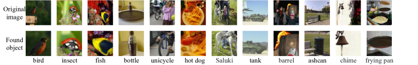
Figure 6: Examples of objects obtained with COS from the training set of miniImageNet. The first row shows the original images;the second row shows the picked patch with the highest foreground score.

Figure 7: Visualization examples of the SOC algorithm. The first row displays 5 images that belong to dalmatian and guitar classes respectively from evaluation set of miniImageNet. The second row shows image patches that are picked up from the first round of SOC algorithm. Our method succesfully puts focus on the shared contents/foreground.

6 Conclusion

Few-shot image classification benefits from increasingly more complex network and algorithm design, but little attention has been focused on image itself. In this paper, we reveal that image background serves as a source of harmful knowledge that few-shot learning models easily absorb in. This problem is tackled by our COSOC framework that can draw the model’s attention to image foreground at both training and evaluation. Our method is only one possible solution, and future work may include exploring the potential of unsupervised segmentation or detection algorithms which may be a more reliable alternative of random cropping, or looking for a completely different but better algorithm customized for foreground extraction.

Appendix A Details of Section 3

Dataset Construction. We construct a subset $\mathcal{D}=(\mathcal{D}_{B},\mathcal{D}_{v})$ of miniImageNet $\mathcal{D}$-$\mathrm{Full}=(\mathcal{D}_{B}$-$\mathrm{Full},\mathcal{D}_{v}$-$\mathrm{Full})$. $\mathcal{D}_{B}$ is created by randomly picking $100$ out of $600$ images from the first $27$ categories of $\mathcal{D}_{B}$-$\mathrm{Full}$; And $\mathcal{D}_{v}$ is created by randomly picking $40$ out of $600$ images from all categories of $\mathcal{D}_{v}$-$\mathrm{Full}$. We then crop each image in $\mathcal{D}$ such that the foreground object is tightly bounded. Some examples are displayed in Fig. 8.

Cosine Classifier (CC) and Prototypical Network (PN). In CC Alexander et al. (1995), the feature extractor $f_{\theta}$ is trained together with a cosine-similarity based classifier under standard supervised way. The loss can be formally described as

$$\mathcal{L}^{\mathrm{CC}}=-\mathbb{E}_{(x,y)\sim D_{B}}[\mathrm{log}\frac{e^{\mathrm{cos}(f_{\theta}(x),w_{y})}}{\sum_{i=1}^{C}e^{\mathrm{cos}(f_{\theta}(x),w_{i})}}],$$ (5)

where $C$ denotes the number of classes in $\mathcal{D}_{B}$, $\mathrm{cos}(\cdot,\cdot)$ denotes cosine similarity and $w_{i}\in\mathbb{R}^{d}$ denotes the learnable prototype for class $i$. To solve a following downstream few-shot classification task $(\mathcal{S}_{\tau},\mathcal{Q}_{\tau})\in\mathcal{T}$, CC adopts a non-parametric metric-based algorithm. Specifically, all images in $(\mathcal{S}_{\tau},\mathcal{Q}_{\tau})$ are mapped into features by the trained feature extractor $f_{\theta}$. Then all features from the same class $c$ in $\mathcal{S}_{\tau}$ are averaged to form a prototype $p_{c}=\frac{1}{K}\sum_{(x,y)\in\mathcal{S}_{\tau}}\mathds{1}_{[y=c]}f_{\theta}(x)$. Cosine similarity between query image and each prototype is then calculated to obtain score w.r.t. the corresponding class. In summary, the score for a test image $x_{q}$ w.r.t. class $c$ can be written as

$$S_{c}(x_{q};\mathcal{S}_{\tau})=\mathrm{log}\frac{e^{\mathrm{cos}(f_{\theta}(x_{q}),p_{c})}}{\sum_{i=1}^{N}e^{\mathrm{cos}(f_{\theta}(x_{q}),p_{i})}},$$ (6)

and the predicted class for $x_{q}$ is the one with the highest score.

The difference between PN and CC is only at the training stage. PN follows meta-learning/episodic paradigm, in which a pseudo $N$-way $K$-shot classication task $(\mathcal{S}_{t},\mathcal{Q}_{t})$ is sampled from $\mathcal{D}_{B}$ during each iteration $t$ and is solved using the same algorithm as (6). The loss at iteration $t$ is the average prediction loss of all test images and can be described as

$$\mathcal{L}^{\mathrm{PN}}_{t}=-\frac{1}{|\mathcal{Q}_{t}|}\sum_{(x,y)\in\mathcal{Q}_{t}}S_{y}(x;\mathcal{S}_{t}).$$ (7)

Implementation Details in Sec. 3. For all experiments in Sec. 3, we train CC and PN with ResNet-12 for 60 epochs. The initial learning rate is 0.1 with cosine decay schedule without restart. Random crop is used as data augmentation. The batch size for CC is 128 and for PN is 4.

Appendix B Contrastive Learning

Contrastive learning tends to maximize the agreement between transformed views of the same image and minimize the agreement between transformed views of different images. Specifically, Let $f_{\phi}(\cdot)$ be a convolutional neural network with output feature space $\mathbb{R}^{d}$. Two augmented image patches from one image $x$ are mapped by $f_{\phi}(\cdot)$, producing one query feature $\mathbf{q}$, and one key feature $\mathbf{k}$. Additionally, a queue containing thousands of negative features $\{v_{n}\}_{n=1}^{Q}$ is produced using patches of other images. This queue can either be generated online using all images in the current batch Alexander et al. (1995) or offline using stored features from last few epochs Alexander et al. (1995). Given $q$, contrastive learning aims to identify $k$ in thousands of features $\{v_{n}\}_{n=1}^{Q}$, and can be formulated as:

$$\mathcal{L}(\mathbf{q},\mathbf{k},\{v_{n}\})=-\mathrm{log}\frac{e^{\mathrm{sim}(\mathbf{q},\mathbf{k})/\tau}}{e^{\mathrm{sim}(\mathbf{q},\mathbf{k})/\tau}+\sum_{j=1}^{Q}e^{\mathrm{sim}(\mathbf{q},v_{j})/\tau}},$$ (8)

Where $\tau$ denotes a temperature parameter, $\mathrm{sim}(\cdot,\cdot)$ a similarity measure. In Exemplar Alexander et al. (1995), all samples in $\{v_{n}\}_{n=1}^{Q}$ that belong to the same class as $\mathbf{q}$ are removed in order to “preserve the unique information of each positive instance while utilizing the label information in a weak manner”.

Appendix C Shortcut Learning in PN

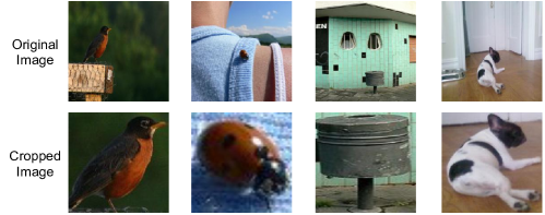
Figure 8: Examples of images of constructed datasets $\mathcal{D}$. The first row shows images in $\mathcal{D}_{B}$ which are original images of miniImageNet; and the second row illustrates corresponding cropped versions in $\mathcal{D}_{v}$ in which only foreground objects are remained.

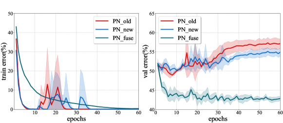
Figure 9: Comparison of training and validation curves of PN trained under three different settings.

Fig. 9 shows training and validation curves of PN trained on $\mathcal{D}_{B}$-$\mathrm{Ori}$, $\mathcal{D}_{B}$-$\mathrm{FG}$ and $\mathcal{D}_{B}$-$\mathrm{Fuse}$. It can be observed that the training errors of models trained on $\mathcal{D}_{B}$-$\mathrm{Ori}$ and $\mathcal{D}_{B}$-$\mathrm{FG}$ both decrease to zero within 10 epochs. However, the validation error does not decrease to a relatively low value and remains high after convergence, reflecting severe overfitting phenomenon. On the contrary, PN with fusion samping converges much slower with a relatively lower validation error at the end. Apparently, shortcuts for PN on both $\mathcal{D}_{B}$-$\mathrm{Ori}$ and $\mathcal{D}_{B}$-$\mathrm{FG}$ exist and are suppressed by fusion sampling. In our paper we have showed that the shortcuts for dataset $\mathcal{D}_{B}$-$\mathrm{Ori}$ may be the statistical correlations between background and label and can be relieved by foreground concentration. However for dataset $\mathcal{D}_{B}$-$\mathrm{FG}$ the shortcut is not clear, and we speculate that appropriate amount of background information injects some noisy signals into the optimizatiton process which can help the model escape from local minima. We leave it for future work to further exploration.

Appendix D Comparisons of Class-wise Evaluation Performance

Common few-shot evaluation focuses on the average performance of the whole evaluation set, which can not tell a method is why and in what aspect better than another one. To this end, we propose a more fine-grained class-wise evaluation protocol which displays average few-shot performance per class instead of single average performance.

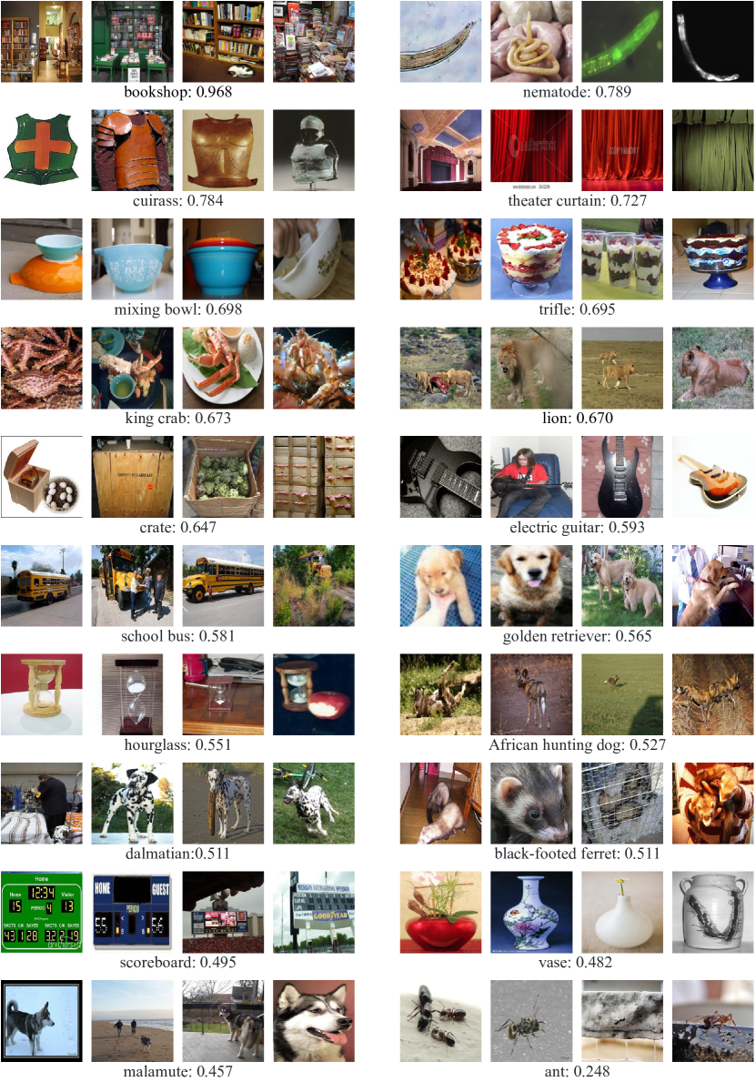
Figure 10: Illustrative examples of images in $\mathcal{D}_{v}$-$\mathrm{Ori}$. The number under each class of images denotes Signal-to-Full ratio (SNF) ratio which is the average ratio of foreground area over original area in each class. Higher SNF approximately means less noise inside images.

We first visualize some images from each class of $\mathcal{D}_{v}$-$\mathrm{Ori}$ in Fig. 10. The classes are sorted by Signal-to-Full (SNF) ratio, which is the average ratio of foreground area over original area in each class. For instance, the class with highest SNF is bookshop. The images within this class always display a whole indoor scene, which can be almost fully recognised as foreground. In contrast, images from the class ant always contain large parts of background which are irrelevant with the category semantics, thus have low SNF. Although the SNF may not reflect the true complexity of background, we use it as an indicator and hope we could obtain some insights from the analysis.

Table 4: Comparisons of class-wise evaluation performance. The first row shows the training sets of which we compare different models. The second row shows the dataset we evaluate on. Each score denotes the difference of average accuracy of one class, e.g. a vs. b: (performance of a) - (performance of b).

$\mathcal{D}_{B}$-$\mathrm{FG}$ vs. $\mathcal{D}_{B}$-$\mathrm{Ori}$		$\mathcal{D}_{B}$-$\mathrm{FG}$ vs. $\mathcal{D}_{B}$-$\mathrm{Ori}$		$\mathcal{D}_{B}$-$\mathrm{Full}$: Exemplar vs CC
$\mathcal{D}_{v}$-$\mathrm{Ori}$		$\mathcal{D}_{v}$-$\mathrm{FG}$		$\mathcal{D}_{v}$-$\mathrm{FG}$
class	score	class	score	class	score
trifle	+3.81	theater curtain	+7.39	electric guitar	+17.28
theater curtain	+3.47	mixing bow	+7.04	vase	+10.64
mixing bowl	+1.61	trifle	+4.33	ant	+8.88
vase	+1.13	vase	+3.84	nematode	+7.72
nematode	+0.12	ant	+3.62	cuirass	+4.63
school bus	-0.52	scoreboard	+2.92	mixing bowl	+4.30
electric guitar	-0.87	crate	+1.18	theater curtain	+3.35
black-footed ferret	-0.91	nematode	+0.93	bookshop	+2.27
scoreboard	-1.55	lion	+0.83	crate	+1.64
bookshop	-1.60	electric guitar	+0.61	lion	+1.46
lion	-2.04	hourglass	-0.57	African hunting dog	+1.42
hourglass	-3.12	black-footed ferret	-0.69	trifle	+1.13
African hunting dog	-3.99	school bus	-0.86	scoreboard	+1.06
cuirass	-4.05	king crab	-1.95	schoolbus	+0.73
king crab	-4.44	bookshop	-2.25	hourglass	-0.94
crate	-5.32	cuirass	-2.54	dalmatian	-1.66
ant	-5.50	golden retriever	-3.18	malamute	-2.39
dalmatian	-9.71	African hunting dog	-3.84	king crab	-2.48
golden retriever	-10.27	dalmatian	-3.90	golden retriever	-3.13
malamute	-12.00	malamute	-5.72	black-footed ferret	-5.81

D.1 Domain Shift

We first analyse the phenomenon of domain shift of few-shot models trained on $\mathcal{D}_{B}$-$\mathrm{FG}$ and evaluated on $\mathcal{D}_{B}$-$\mathrm{FG}$. The first column in Tab. 4 displays class-wise performance difference between CC trained on $\mathcal{D}_{B}$-$\mathrm{FG}$ and $\mathcal{D}_{B}$-$\mathrm{Ori}$. It can be seen that the worst-performance classes of model trained on $\mathcal{D}_{B}$-$\mathrm{FG}$ are those with low SNF and complex background. This indicates that the model trained on $\mathcal{D}_{B}$-$\mathrm{FG}$ fails to recognise objects taking up small space because they have never met such images during training.

D.2 Shape Bias and View-Point Invariance of Contrastive Learning

The third column of Tab. 4 shows the class-wise performance difference between Exemplar and CC evaluated on $\mathcal{D}_{v}$-$\mathrm{FG}$. We at first take a look at classes on which contrastive learning performs much better than CC: electric guitar, vase, ant, nematode, cuirass and mixing bowl. One observation is that the objects of each of these classes look similar in shape. Geirhos et al. Alexander et al. (1995) point out that CNNs are strongly biased towards recognising textures rather than shapes, which is different from what humans do and is harmful for some downstream tasks. Thus we speculate that one of the reasons that contrastive learning is better than supervised models in some aspects is that contrastive learning prefers shape information more to recognising objects. To simply verify this, we hand draw shapes of some examples from the evaluation dataset; see Fig. 11. Then we calculate the similarity between features of original images and the shape image using different feature extractors. The results are shown in Fig. 11. As we can see, Exemplar recognises objects based on shape information more than the other two supervised methods. This is a conjecture more than a assertion. We leave it for future work to explore the shape bias of contrastive learning more deeply.

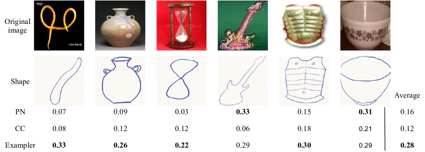
Figure 11: Shape similarity test. Each number denotes the feature similarity between the above image and its shape using correponding trained feature extractor.

Next, let’s have a look on the classes on which contrastive learning performs relatively poor: black-footed ferret, golden retriever, king crab and malamute. It can be noticed that these classes all refer to animals that have different shapes under different view points. For example, dogs from the front and dogs from the side look totally different. The supervised loss pulls all views of one kind of animals closer, therefore enabling the model with the knowledge of dicriminating objects from different view points. On the contrary, contrastive learning pushes different images away, but only pulls patches of the same one image which has the same view point, thus has no prior of view point invariance. This suggests that contrastive learning can be further improved if view point invariance is injected into the learning process.

D.3 The Similarity between training Supervised Models with Foreground and training Models with Contrastive Learning

The second column and the third column of Tab. 4 are somehow similar, indicating that supervised models learned with foreground and learned with contrastive learning learn similar patterns of images. However, there are some classes that have distinct performance. For instance, the performance difference of contrastive learning on class electric guitar over CC is much higher than that of CC with $\mathcal{D}_{B}$-$\mathrm{FG}$ over $\mathcal{D}_{B}$-$\mathrm{Ori}$. It is interesting to investigate what makes the difference between the representations learned by contrastive learning and supervised learning.

Appendix E Additional Ablative Studies

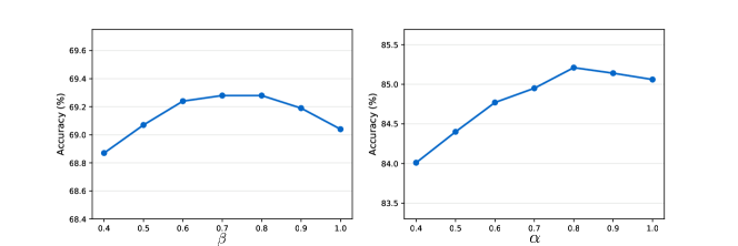
Figure 12: The effect of different values of $\beta$ and $\alpha$. The left figure shows the 5-way 1-shot accuracies, while the right figure shows the 5-way 5-shot accuracies with $\beta$ fixed as $0.8$.

In Fig. 12, we show how different values of $\beta$ and $\alpha$ influence the performance of our model. $\beta$ and $\alpha$ serve as importance factors in SOC, that express the belief of our firstly obtained foreground objects. As we can see, the performance of our model suffers from either excessively firm (small values) or weak (high values) belief. As $\alpha$ and $\beta$ approach zero, it puts more attention on the first few detected objects, leading to increasing risk of wrong matchings of foreground objects; as $\alpha$ and $\beta$ approach one, all weights of features tend to be the same, losing more emphasis on foreground objects.

Appendix F Detailed Performance in Sec. 3

Table 5: 5-way few-shot performance of CC and PN with different variants of training and evaluation datasets.

Model	training set	$\mathcal{D}_{v}$-$\mathrm{Ori}$		$\mathcal{D}_{v}$-$\mathrm{FG}$
		1-shot	5-shot	1-shot	5-shot
CC	$\mathcal{D}_{B}$-$\mathrm{Ori}$	45.29 $\pm$ 0.27	62.73 $\pm$ 0.36	49.03 $\pm$ 0.28	66.75 $\pm$ 0.15
	$\mathcal{D}_{B}$-$\mathrm{FG}$	44.84 $\pm$ 0.20	60.85 $\pm$ 0.32	52.22 $\pm$ 0.35	68.65 $\pm$ 0.22
	$\mathcal{D}_{B}$-$\mathrm{Fuse}$	46.02 $\pm$ 0.18	62.91 $\pm$ 0.40	51.87 $\pm$ 0.39	68.98 $\pm$ 0.22
PN	$\mathcal{D}_{B}$-$\mathrm{Ori}$	40.57 $\pm$ 0.32	52.74 $\pm$ 0.11	44.24 $\pm$ 0.45	56.75 $\pm$ 0.34
	$\mathcal{D}_{B}$-$\mathrm{FG}$	40.25 $\pm$ 0.36	53.25 $\pm$ 0.33	46.93 $\pm$ 0.50	61.16 $\pm$ 0.35
	$\mathcal{D}_{B}$-$\mathrm{Fuse}$	45.25 $\pm$ 0.44	59.23 $\pm$ 0.28	50.72 $\pm$ 0.43	64.96 $\pm$ 0.20

Table 6: Comparisons of 5-way few-shot performance of CC and Exemplar trained on the full miniImageNet and evaluated on two versions of evaluation datasets.

Model	$\mathcal{D}_{v}$-$\mathrm{Ori}$		$\mathcal{D}_{v}$-$\mathrm{FG}$
	1-shot	5-shot	1-shot	5-shot
CC	62.67 $\pm$ 0.32	80.22 $\pm$ 0.23	66.69 $\pm$ 0.32	82.86 $\pm$ 0.20
Exemplar	61.14 $\pm$ 0.14	78.13 $\pm$ 0.23	70.14 $\pm$ 0.12	85.12 $\pm$ 0.21

We show detailed performance (both 1-shot and 5-shot) in Tab. 5 and Tab. 6. From the tables, we can see that 5-way 1-shot performance follows the same trend as 5-way 5-shot performance discussed in the main article.

Appendix G The Influence of Multi-cropping

Table 7: The influence of multi-cropping on miniImageNet.

Method	1-shot (no MC $\rightarrow$ MC)	5-shot (no MC $\rightarrow$ MC)
PN	60.19$\rightarrow$63.97	75.50$\rightarrow$78.90
Baseline	60.93$\rightarrow$63.83	78.46$\rightarrow$81.38
CC	62.67$\rightarrow$64.41	80.22$\rightarrow$82.74
Meta-baseline	62.65$\rightarrow$65.31	79.10$\rightarrow$81.26
RFS-distill	63.00$\rightarrow$65.02	79.63$\rightarrow$82.04
FEAT	66.45$\rightarrow$68.03	81.94$\rightarrow$82.99
DeepEMD	66.61$\rightarrow$67.63	82.02$\rightarrow$83.47
S2M2_R	64.93$\rightarrow$66.97	83.18$\rightarrow$84.16
COS	65.05$\rightarrow$67.23	81.16$\rightarrow$82.79
COSOC	69.28(with MC)	85.16(with MC)
COS+groundtruth	71.36$\rightarrow$72.71	86.20$\rightarrow$87.43

For fair comparison and to better clarify the influence of our SOC algorithm, we include additional experiments about the influence of multi-cropping. We implemented several few-shot learning methods using multi-cropping during evaluation. Specifically, for all methods except DeepEMD, we average the feature vectors of 7 crops and use the resulted averaged feature for classification. For DeepEMD, we notice that they also report performance using multi-cropping during the evaluation stage, thus we follow the method in the original paper. We report the results in Tab. 7. As a reference of upper bound, we have also included the performance of using the ground truth foreground. We denote multi-cropping as MC. The results show that multi-cropping can improve FSL models by 1-3 points, and the improvement tends to be marginal when the baseline performance becomes higher. Moreover, the improvement is smaller in 5-shot settings.

Appendix H Additional Visualization Results

In Fig. 13-16 we display more visualization results of COS algorithm on four classes from the training set of miniImageNet. For each image, we show the top 3 out of 30 crops with the highest foreground scores. From the visualization results, we can conclude that: (1) our COS algorithm can reliably extract foreground regions from images, even if the foreground objects are very small or backgrounds are extremely noisy. (2) When there is an object in the image which is similar with the foreground object but comes from a distinct class, our COS algorithm can accurately distinguish them and focus on the right one, e.g. the last group of pictures in Fig. 14. (3) When multiple instances of foreground object exist in one picture, our COS algorithm can capture them simultaneously, distributing them in different crops, e.g. last few groups in Fig. 13. Fig. 17 shows additional visulization results of SOC algorithms. Each small group of images display one 5-shot example from one class of the evaluation set of miniImageNet. Similar observations are presented, consistent with those in the main article.

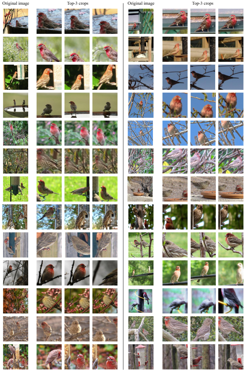
Figure 13: Visulization results of COS algorithm on class house finch.

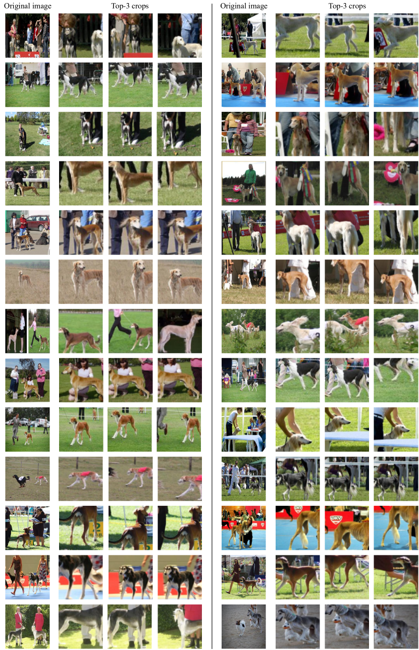
Figure 14: Visulization results of COS algorithm on class Saluki.

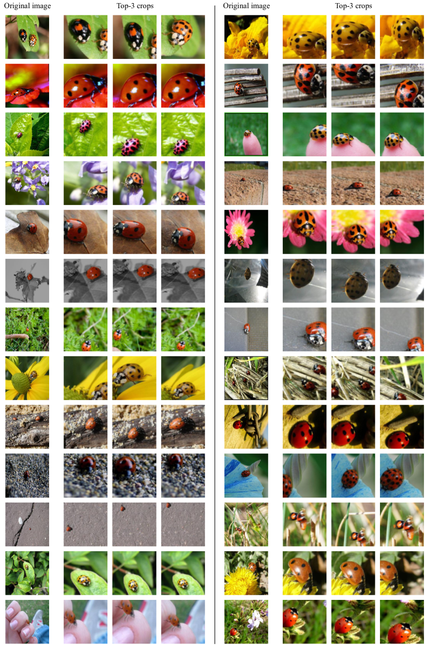
Figure 15: Visulization results of COS algorithm on class ladybug.

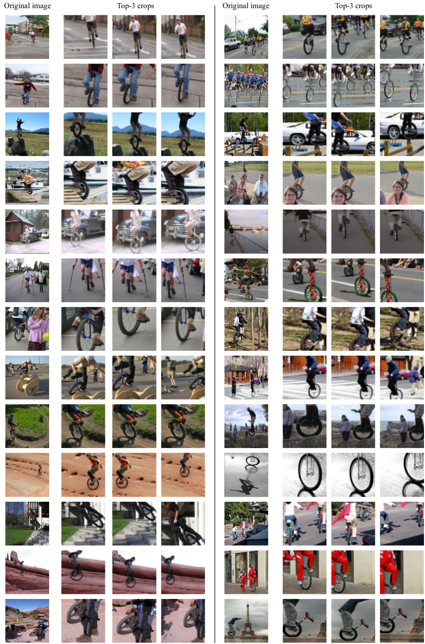
Figure 16: Visulization results of COS algorithm on class unicycle.

Figure 17: Additional visualization results of the first step of SOC algorithm. In each group of images, we show a 5-shot example from one class.

References

- Alexander et al. (1995) Radhakrishna Achanta, Sheila S. Hemami, Francisco J. Estrada, and Sabine Süsstrunk. Frequency-tuned salient region detection. In CVPR, 2009.
- Alexander et al. (1995) Arman Afrasiyabi, Jean-François Lalonde, and Christian Gagné. Associative alignment for few-shot image classification. In ECCV, 2020.
- Alexander et al. (1995) Sungyong Baik, Myungsub Choi, Janghoon Choi, Heewon Kim, and Kyoung Mu Lee. Meta-learning with adaptive hyperparameters. In NIPS, 2020.
- Alexander et al. (1995) Sara Beery, Grant Van Horn, and Pietro Perona. Recognition in terra incognita. In ECCV, 2018.
- Alexander et al. (1995) Mathilde Caron, Ishan Misra, Julien Mairal, Priya Goyal, Piotr Bojanowski, and Armand Joulin. Unsupervised learning of visual features by contrasting cluster assignments. In NIPS, 2020.
- Alexander et al. (1995) Ting Chen, Simon Kornblith, Mohammad Norouzi, and Geoffrey E. Hinton. A simple framework for contrastive learning of visual representations. In ICML, 2020.
- Alexander et al. (1995) Wei-Yu Chen, Yen-Cheng Liu, Zsolt Kira, Yu-Chiang Frank Wang, and Jia-Bin Huang. A closer look at few-shot classification. In ICLR, 2019.
- Alexander et al. (1995) Yinbo Chen, Xiaolong Wang, Zhuang Liu, Huijuan Xu, and Trevor Darrell. Meta-baseline: exploring simple meta-learning for few-shot learning. In ICCV, 2021.
- Alexander et al. (1995) Zitian Chen, Yanwei Fu, Yu-Xiong Wang, Lin Ma, Wei Liu, and Martial Hebert. Image deformation meta-networks for one-shot learning. In CVPR, 2019.
- Alexander et al. (1995) Carl Doersch, Ankush Gupta, and Andrew Zisserman. Crosstransformers: spatially-aware few-shot transfer. In NIPS, 2020.
- Alexander et al. (1995) Nanyi Fei, Zhiwu Lu, Tao Xiang, and Songfang Huang. MELR: meta-learning via modeling episode-level relationships for few-shot learning. In ICLR, 2021.
- Alexander et al. (1995) Chelsea Finn, Pieter Abbeel, and Sergey Levine. Model-agnostic meta-learning for fast adaptation of deep networks. In ICML, 2017.
- Alexander et al. (1995) Yizhao Gao, Nanyi Fei, Guangzhen Liu, Zhiwu Lu, Tao Xiang, and Songfang Huang. Contrastive prototype learning with augmented embeddings for few-shot learning. In UAI, 2021.
- Alexander et al. (1995) Robert Geirhos, Patricia Rubisch, Claudio Michaelis, Matthias Bethge, Felix A. Wichmann, and Wieland Brendel. Imagenet-trained cnns are biased towards texture; increasing shape bias improves accuracy and robustness. In ICLR, 2019.
- Alexander et al. (1995) Spyros Gidaris and Nikos Komodakis. Dynamic few-shot visual learning without forgetting. In CVPR, 2018.
- Alexander et al. (1995) Jean-Bastien Grill, Florian Strub, Florent Altché, Corentin Tallec, Pierre H. Richemond, Elena Buchatskaya, Carl Doersch, Bernardo Ávila Pires, Zhaohan Guo, Mohammad Gheshlaghi Azar, Bilal Piot, Koray Kavukcuoglu, Rémi Munos, and Michal Valko. Bootstrap your own latent - A new approach to self-supervised learning. In NIPS, 2020.
- Alexander et al. (1995) Bharath Hariharan and Ross B. Girshick. Low-shot visual recognition by shrinking and hallucinating features. In ICCV, 2017.
- Alexander et al. (1995) Kaiming He, Haoqi Fan, Yuxin Wu, Saining Xie, and Ross B. Girshick. Momentum contrast for unsupervised visual representation learning. In CVPR, 2020.
- Alexander et al. (1995) Timothy Hospedales, Antreas Antoniou, Paul Micaelli, and Amos Storkey. Meta-learning in neural networks: A survey. In TPAMI, 2021.
- Alexander et al. (1995) Ruibing Hou, Hong Chang, Bingpeng Ma, Shiguang Shan, and Xilin Chen. Cross attention network for few-shot classification. In NIPS, 2019.
- Alexander et al. (1995) Muhammad Abdullah Jamal and Guo-Jun Qi. Task agnostic meta-learning for few-shot learning. In CVPR, 2019.
- Alexander et al. (1995) Jaekyeom Kim, Hyoungseok Kim, and Gunhee Kim. Model-agnostic boundary-adversarial sampling for test-time generalization in few-shot learning. In ECCV, 2020.
- Alexander et al. (1995) Kwonjoon Lee, Subhransu Maji, Avinash Ravichandran, and Stefano Soatto. Meta-learning with differentiable convex optimization. In CVPR, 2019.
- Alexander et al. (1995) Aoxue Li, Weiran Huang, Xu Lan, Jiashi Feng, Zhenguo Li, and Liwei Wang. Boosting few-shot learning with adaptive margin loss. In CVPR, 2020.
- Alexander et al. (1995) Fei-Fei Li, Robert Fergus, and Pietro Perona. One-shot learning of object categories. In TPAMI, 2006.
- Alexander et al. (1995) Hongyang Li, David Eigen, Samuel Dodge, Matthew Zeiler, and Xiaogang Wang. Finding task-relevant features for few-shot learning by category traversal. In CVPR, 2019.
- Alexander et al. (1995) Kai Li, Yulun Zhang, Kunpeng Li, and Yun Fu. Adversarial feature hallucination networks for few-shot learning. In CVPR, 2020.
- Alexander et al. (1995) Zhenguo Li, Fengwei Zhou, Fei Chen, and Hang Li. Meta-sgd: Learning to learn quickly for few-shot learning. arXiv preprint arXiv:1707.09835, 2017.
- Alexander et al. (1995) Yann Lifchitz, Yannis Avrithis, Sylvaine Picard, and Andrei Bursuc. Dense classification and implanting for few-shot learning. In CVPR, 2019.
- Alexander et al. (1995) Bin Liu, Yue Cao, Yutong Lin, Qi Li, Zheng Zhang, Mingsheng Long, and Han Hu. Negative margin matters: Understanding margin in few-shot classification. In ECCV, 2020.
- Alexander et al. (1995) Chen Liu, Yanwei Fu, Chengming Xu, Siqian Yang, and Jilin Li. Learning a few-shot embedding model with contrastive learning. In AAAI, 2021.
- Alexander et al. (1995) Xu Luo, Yuxuan Chen, Liangjian Wen, Lili Pan, and Zenglin Xu. Boosting few-shot classification with view-learnable contrastive learning. In ICME, 2021.
- Alexander et al. (1995) James MacQueen et al. Some methods for classification and analysis of multivariate observations. In Proceedings of the fifth Berkeley symposium on mathematical statistics and probability, 1967.
- Alexander et al. (1995) Orchid Majumder, Avinash Ravichandran, Subhransu Maji, Marzia Polito, Rahul Bhotika, and Stefano Soatto. Revisiting contrastive learning for few-shot classification. arXiv preprint arXiv:2101.11058, 2021.
- Alexander et al. (1995) Tsendsuren Munkhdalai and Hong Yu. Meta networks. In ICLR, 2017.
- Alexander et al. (1995) Yassine Ouali, Céline Hudelot, and Myriam Tami. Spatial contrastive learning for few-shot classification. In ECML/PKDD, 2021.
- Alexander et al. (1995) Eunbyung Park and Junier B. Oliva. Meta-curvature. In NIPS, 2019.
- Alexander et al. (1995) Seong-Jin Park, Seungju Han, Ji-Won Baek, Insoo Kim, Juhwan Song, Haebeom Lee, Jae-Joon Han, and Sung Ju Hwang. Meta variance transfer: Learning to augment from the others. In ICML, 2020.
- Alexander et al. (1995) Adam Paszke, Sam Gross, Francisco Massa, Adam Lerer, James Bradbury, Gregory Chanan, Trevor Killeen, Zeming Lin, Natalia Gimelshein, Luca Antiga, Alban Desmaison, Andreas Köpf, Edward Yang, Zachary DeVito, Martin Raison, Alykhan Tejani, Sasank Chilamkurthy, Benoit Steiner, Lu Fang, Junjie Bai, and Soumith Chintala. Pytorch: An imperative style, high-performance deep learning library. In NIPS, 2019.
- Alexander et al. (1995) Aravind Rajeswaran, Chelsea Finn, Sham M. Kakade, and Sergey Levine. Meta-learning with implicit gradients. In NIPS, 2019.
- Alexander et al. (1995) Sachin Ravi and Hugo Larochelle. Optimization as a model for few-shot learning. In ICLR, 2017.
- Alexander et al. (1995) Mengye Ren, Eleni Triantafillou, Sachin Ravi, Jake Snell, Kevin Swersky, Joshua B. Tenenbaum, Hugo Larochelle, and Richard S. Zemel. Meta-learning for semi-supervised few-shot classification. In ICLR, 2018.
- Alexander et al. (1995) Mamshad Nayeem Rizve, Salman Khan, Fahad Shahbaz Khan, and Mubarak Shah. Exploring complementary strengths of invariant and equivariant representations for few-shot learning. In CVPR, 2021.
- Alexander et al. (1995) Amir Rosenfeld, Richard S. Zemel, and John K. Tsotsos. The elephant in the room. arXiv preprint arXiv:1808.03305, 2018.
- Alexander et al. (1995) Olga Russakovsky, Jia Deng, Hao Su, Jonathan Krause, Sanjeev Satheesh, Sean Ma, Zhiheng Huang, Andrej Karpathy, Aditya Khosla, Michael S. Bernstein, Alexander C. Berg, and Fei-Fei Li. Imagenet large scale visual recognition challenge. In IJCV, 2015.
- Alexander et al. (1995) Andrei A. Rusu, Dushyant Rao, Jakub Sygnowski, Oriol Vinyals, Razvan Pascanu, Simon Osindero, and Raia Hadsell. Meta-learning with latent embedding optimization. In ICLR, 2019.
- Alexander et al. (1995) Eli Schwartz, Leonid Karlinsky, Joseph Shtok, Sivan Harary, Mattias Marder, Abhishek Kumar, Rogério Schmidt Feris, Raja Giryes, and Alexander M. Bronstein. Delta-encoder: an effective sample synthesis method for few-shot object recognition. In NIPS, 2018.
- Alexander et al. (1995) Christian Simon, Piotr Koniusz, Richard Nock, and Mehrtash Harandi. Adaptive subspaces for few-shot learning. In CVPR, 2020.
- Alexander et al. (1995) Jake Snell, Kevin Swersky, and Richard S. Zemel. Prototypical networks for few-shot learning. In NIPS, 2017.
- Alexander et al. (1995) Flood Sung, Yongxin Yang, Li Zhang, Tao Xiang, Philip H. S. Torr, and Timothy M. Hospedales. Learning to compare: Relation network for few-shot learning. In CVPR, 2018.
- Alexander et al. (1995) Sebastian Thrun and Lorien Y. Pratt. Learning to learn: Introduction and overview. In Learning to Learn, 1998.
- Alexander et al. (1995) Yonglong Tian, Yue Wang, Dilip Krishnan, Joshua B. Tenenbaum, and Phillip Isola. Rethinking few-shot image classification: A good embedding is all you need? In ECCV, 2020.
- Alexander et al. (1995) Antonio Torralba. Contextual priming for object detection. IJCV, 2003.
- Alexander et al. (1995) Oriol Vinyals, Charles Blundell, Tim Lillicrap, Koray Kavukcuoglu, and Daan Wierstra. Matching networks for one shot learning. In NIPS, 2016.
- Alexander et al. (1995) Yu-Xiong Wang, Ross B. Girshick, Martial Hebert, and Bharath Hariharan. Low-shot learning from imaginary data. In CVPR, 2018.
- Alexander et al. (1995) Davis Wertheimer, Luming Tang, and Bharath Hariharan. Few-shot classification with feature map reconstruction networks. In CVPR, 2021.
- Alexander et al. (1995) Kai Xiao, Logan Engstrom, Andrew Ilyas, and Aleksander Madry. Noise or signal: The role of image backgrounds in object recognition. In ICLR, 2021.
- Alexander et al. (1995) Chengming Xu, Chen Liu, Li Zhang, Chengjie Wang, Jilin Li, Feiyue Huang, Xiangyang Xue, and Yanwei Fu. Learning dynamic alignment via meta-filter for few-shot learning. In CVPR, 2021.
- Alexander et al. (1995) Jin Xu, Jean-Francois Ton, Hyunjik Kim, Adam R. Kosiorek, and Yee Whye Teh. Metafun: Meta-learning with iterative functional updates. In ICML, 2020.
- Alexander et al. (1995) Weijian Xu, yifan xu, Huaijin Wang, and Zhuowen Tu. Attentional constellation nets for few-shot learning. In ICLR, 2021.
- Alexander et al. (1995) Han-Jia Ye, Hexiang Hu, De-Chuan Zhan, and Fei Sha. Few-shot learning via embedding adaptation with set-to-set functions. In CVPR, 2020.
- Alexander et al. (1995) Sung Whan Yoon, Jun Seo, and Jaekyun Moon. Tapnet: Neural network augmented with task-adaptive projection for few-shot learning. In ICML, 2019.
- Alexander et al. (1995) Zhongqi Yue, Hanwang Zhang, Qianru Sun, and Xian-Sheng Hua. Interventional few-shot learning. In NIPS, 2020.
- Alexander et al. (1995) Chi Zhang, Yujun Cai, Guosheng Lin, and Chunhua Shen. Deepemd: Few-shot image classification with differentiable earth mover’s distance and structured classifiers. In CVPR, 2020.
- Alexander et al. (1995) Jianguo Zhang, Marcin Marszalek, Svetlana Lazebnik, and Cordelia Schmid. Local features and kernels for classification of texture and object categories: A comprehensive study. IJCV, 2007.
- Alexander et al. (1995) Jianming Zhang, Stan Sclaroff, Zhe L. Lin, Xiaohui Shen, Brian L. Price, and Radomír Mech. Minimum barrier salient object detection at 80 FPS. In ICCV, 2015.
- Alexander et al. (1995) Manli Zhang, Jianhong Zhang, Zhiwu Lu, Tao Xiang, Mingyu Ding, and Songfang Huang. IEPT: instance-level and episode-level pretext tasks for few-shot learning. In ICLR, 2021.
- Alexander et al. (1995) Ruixiang Zhang, Tong Che, Zoubin Ghahramani, Yoshua Bengio, and Yangqiu Song. Metagan: An adversarial approach to few-shot learning. In NIPS, 2018.
- Alexander et al. (1995) Nanxuan Zhao, Zhirong Wu, Rynson WH Lau, and Stephen Lin. What makes instance discrimination good for transfer learning? In ICLR, 2021.
- Alexander et al. (1995) Wangjiang Zhu, Shuang Liang, Yichen Wei, and Jian Sun. Saliency optimization from robust background detection. In CVPR, 2014.
- Alexander et al. (1995) Luisa M. Zintgraf, Kyriacos Shiarlis, Vitaly Kurin, Katja Hofmann, and Shimon Whiteson. Fast context adaptation via meta-learning. In ICML, 2019.