Constrained Feedforward Neural Network Training
via Reachability Analysis

Abstract

Neural networks have recently become popular for a wide variety of uses, but have seen limited application in safety-critical domains such as robotics near and around humans. This is because it remains an open challenge to train a neural network to obey safety constraints. Most existing safety-related methods only seek to verify that already-trained networks obey constraints, requiring alternating training and verification. Instead, this work proposes a constrained method to simultaneously train and verify a feedforward neural network with rectified linear unit (ReLU) nonlinearities. Constraints are enforced by computing the network’s output-space reachable set and ensuring that it does not intersect with unsafe sets; training is achieved by formulating a novel collision-check loss function between the reachable set and unsafe portions of the output space. The reachable and unsafe sets are represented by constrained zonotopes, a convex polytope representation that enables differentiable collision checking. The proposed method is demonstrated successfully on a network with one nonlinearity layer and $\approx 50$ parameters.

I Introduction

Neural networks are a popular method for approximating nonlinear functions, with increasing applications in the field of human-robot interactions. For example, the kinematics of many elder-care robots [1, 2], rehabilitation robots [3, 4], industrial robot manipulators [5], and automated driving systems [6, 7] are controlled by neural networks. Thus, verifying the safety of the neural networks in these systems, before deployment near humans, is crucial in avoiding injuries and accidents. However, it remains an active area of research to ensure the output of a neural network satisfies user-specified constraints and requirements. In this short paper, we take preliminary steps towards safety via constrained training by representing constraints as a collision check between the reachable set of a neural network and unsafe sets in its output space.

I-A Related Work

Many different solutions have been proposed for the verification problem, with set-based reachability analysis being the most common for an uncertain set of inputs [8]. Depending on one’s choice of representation, the predicted output is either exact (e.g. star set [9, 6], ImageStar [10]) or an over-approximation (e.g. zonotope [11]) of the actual output set. Reachability is most commonly computed layer-by-layer, though methods have been proposed that speed up verification by, e.g., using an anytime algorithm to return unsafe cells while enumerating polyhedral cells in the input space [12], or recursively partitioning the input set via shadow prices [13].

Verification techniques have several drawbacks. First, they do not provide feedback about constraints during training, so one must alternate training and verification until desired properties have been achieved. Furthermore, verification by over-approximation can often be inconclusive, while exact verification can be expensive to compute.

Several alternative approaches have therefore been proposed. For example, [14] employs a constrained optimization layer to use the output of the network as a potential function for optimization while enforcing constraints. Similarly, [15, 16] adds a constraint violation penalty to the objective loss function and penalizes violation of the constraint. These methods augment their networks with constrained optimization, but are unable to guarantee constraint satisfaction upon convergence of the training. Alternatively, [17] uses a systematic process of small changes to conform a “mostly-correct” network to constraints. However the method only works for networks with a Two-Level Lattice (TLL) architecture, requires an already-trained network, and again does not guarantee a provably safe solution. Finally, [18] attempts to learn the optimal cost-to-go for the Hamilton–Jacobi–Bellman (HJB) equation, while subjected to constraints on the output of the neural network controller. Yet, it does not actually involve any network training and is unable to handle uncertain input sets.

Recently, constrained zonotopes have been introduced as a set-based representation that is closed under linear transformations and can exactly represent any convex polytope [19, 20]. Importantly, these sets are well-suited for reachability analysis due to analytical, efficient methods for computing Minkowski sums, intersections, and collision checks; in particular, collision-checking only requires solving a linear program. We leverage these properties to enable our contributions.

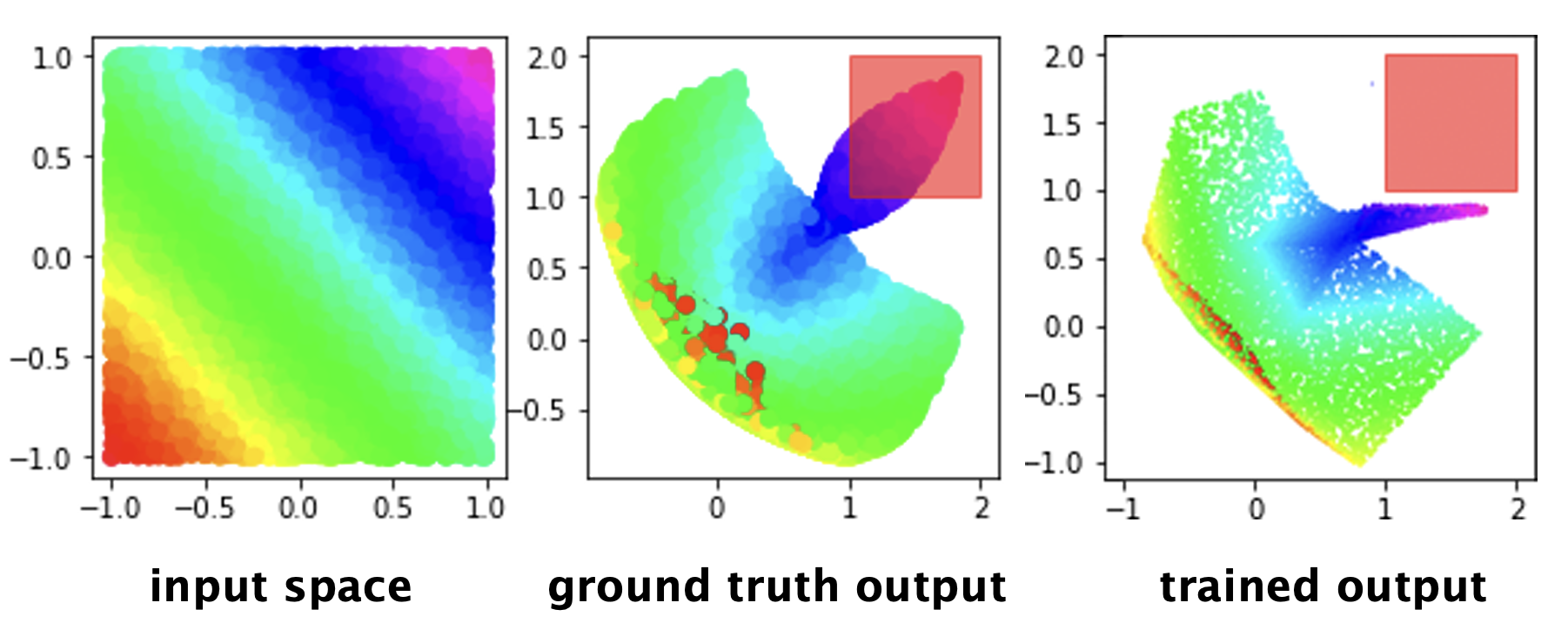
Figure 1: An example safe training result with the proposed method. The color gradient illustrates corresponding input and output points. With our method, the trained output does not intersect the unsafe set (red box).

I-B Contributions

We propose a method to compute the output of a neural network with rectified linear unit (ReLU) activations given an input set represented as constrained zonotopes. We then enforce performance by training under a differentiable zonotope intersection constraint, which guarantees safety upon convergence. Our method is demonstrated on a small numerical example, and illustrated in Fig. 1.

II Preliminaries

We now introduce our notation for neural networks and define constrained zonotopes.

In this work, we consider a fully-connected, ReLU-activated feedforward neural network $\mathbf{n}\!\left(\cdot\right):X^{(0)}\to\mathbb{R}^{n^{(0pt)}}$, with output $\mathbf{x}^{(0pt)}=\mathbf{n}\!\left(\mathbf{x}^{(0)}\right)$ given an input $\mathbf{x}^{(0)}\in X^{(0)}\subset\mathbb{R}^{n^{(0)}}$. We call $X^{(0)}$ the input set. We denote by $0pt\in\mathbb{N}$ the depth of the network and by $n^{(i)}$ the width of the $i$^th layer. For each layer $k=1,\cdots,0pt-1$, the hidden state of the neural network is given by

$$\mathbf{x}^{(k)}=\varrho\!\left(\mathcal{L}\!\left(\mathbf{x}^{(k-1)},\mathbf{W}^{(k-1)},\mathbf{w}^{(k-1)}\right)\right),$$ (1)

where $\mathbf{W}^{(k-1)}\in\mathbb{R}^{n^{(k-1)}\times n^{(k)}}$, $\mathbf{x}^{(k)}$ and $\mathbf{w}^{(k-1)}\in\mathbb{R}^{n^{(k)}}$, and

$$\mathcal{L}\!\left(\mathbf{x},\mathbf{W},\mathbf{w}\right) =\mathbf{W}\mathbf{x}+\mathbf{w},$$ (2)

$$\varrho\!\left(\mathbf{x}\right) =\max\{0,\mathbf{x}\},$$ (3)

where $\mathcal{L}\!\left(\cdot\right)$ is a linear layer operation, and $\varrho\!\left(\cdot\right)$ is the ReLU nonlinearity with the max taken elementwise. We do not apply the ReLU activation for the final output layer:

$$\mathbf{x}^{(0pt)}=\mathcal{L}\!\left(\mathbf{x}^{(0pt)},\mathbf{W}^{(0pt)},\mathbf{w}^{(0pt)}\right).$$ (4)

The reachable set of the neural network is

$$X^{(0pt)}=\mathbf{n}\!\left(X^{(0)}\right)\subset\mathbb{R}^{n^{(0pt)}}.$$ (5)

We represent the reachable set as a union of constrained zonotopes. A constrained zonotope $\mathcal{CZ}\!\left(\mathbf{c},\mathbf{G},\mathbf{A},\mathbf{b}\right)\subset\mathbb{R}^{n}$ is a set parameterized by a center $\mathbf{c}\in\mathbb{R}^{n}$, generator matrix $\mathbf{G}\in\mathbb{R}^{n\times{n_{\mathrm{\textnormal{gen}}}}}$, linear constraints $\mathbf{A}\in\mathbb{R}^{{n_{\mathrm{\textnormal{con}}}}\times{n_{\mathrm{\textnormal{gen}}}}}$, $\mathbf{b}\in\mathbb{R}^{n_{\mathrm{\textnormal{con}}}}$, and coefficients $\mathbf{z}\in\mathbb{R}^{n_{\mathrm{\textnormal{gen}}}}$ as follows:

$$\mathcal{CZ}\!\left(\mathbf{c},\mathbf{G},\mathbf{A},\mathbf{b}\right)=\left\{\mathbf{c}+\mathbf{G}\mathbf{z}\ |\ \left\|\mathbf{z}\right\|_{\infty}\leq 1,\ \mathbf{A}\mathbf{z}=\mathbf{b}\right\}.$$ (6)

Importantly, the intersection of constrained zonotopes is also a constrained zonotope [19, Proposition 1]. Let $Z_{1}=\mathcal{CZ}\!\left(\mathbf{c}_{1},\mathbf{G}_{1},\mathbf{A}_{1},\mathbf{b}_{1}\right)$ and $Z_{2}=\mathcal{CZ}\!\left(\mathbf{c}_{2},\mathbf{G}_{2},\mathbf{A}_{2},\mathbf{b}_{2}\right)$. Then $Z_{1}\cap Z_{2}$ is given by

$$Z_{1}\cap Z_{2}=\mathcal{CZ}\!\left(\mathbf{c}_{1},[\mathbf{G}_{1},\mathbf{0}],\begin{bmatrix}\mathbf{A}_{1}&\mathbf{0}\\ \mathbf{0}&\mathbf{A}_{2}\\ \mathbf{G}_{1}&-\mathbf{G}_{2}\end{bmatrix},\begin{bmatrix}\mathbf{b}_{1}\\ \mathbf{b}_{2}\\ \mathbf{c}_{2}-\mathbf{c}_{1}\end{bmatrix}\right).$$ (7)

We leverage this property to evaluate constraints on the forward reachable set of our neural network.

III Method

In this section, we first explain how to pass a constrained zonotope exactly through a ReLU nonlinearity; that is, we compute the reachable set of a ReLU activation given a constrained zonotope as the input. We then discuss how to train a neural network using the reachable set to enforce constraints. Finally, we explain how to compute the gradient of the constraint for backpropagation.

Before proceeding, we briefly mention that we can pass an input constrained zonotope $Z=\mathcal{CZ}\!\left(\mathbf{c},\mathbf{G},\mathbf{A},\mathbf{b}\right)$ through a linear layer as

$$\mathcal{L}\!\left(Z,\mathbf{W},\mathbf{w}\right)=\mathcal{CZ}\!\left(\mathbf{W}\mathbf{c}+\mathbf{w},\mathbf{W}\mathbf{G},\mathbf{A},\mathbf{b}\right).$$ (8)

This follows from the definition in (6).

III-A Constrained Zonotope ReLU Activation

Proposition 1.

The ReLU activation of a constrained zonotope $Z\subset\mathbb{R}^{n}$ is:

$$\varrho\!\left(Z\right)=\bigcup_{i=1}^{2^{n}}\mathcal{CZ}\!\left(\mathbf{c}^{(i)},\mathbf{G}^{(i)},\mathbf{A}^{(i)},\mathbf{b}^{(i)}\right),$$ (9)

where each output constrained zonotopes is given by:

$$\mathbf{G}^{(i)} =[\mathrm{\textnormal{diag}}\!\left(\mathbf{u}_{i}\right)\mathbf{G},\ \mathbf{0}_{n\times n}],$$ (10a)

$$\mathbf{A}^{(i)} =\begin{bmatrix}\mathbf{A}&\mathbf{0}_{{n_{\mathrm{\textnormal{con}}}}\times n}\\ \mathrm{\textnormal{diag}}\!\left(\mathbf{1}_{n\times 1}-2\mathbf{u}_{i}\right)\mathbf{G}&\mathrm{\textnormal{diag}}\!\left(\mathbf{d}^{(i)}\right)\end{bmatrix},$$ (10b)

$$\mathbf{c}^{(i)} =\mathrm{\textnormal{diag}}\!\left(\mathbf{u}_{i}\right)\mathbf{c},$$ (10c)

$$\mathbf{b}^{(i)} =\begin{bmatrix}\mathbf{b}\\ -\mathrm{\textnormal{diag}}\!\left(\mathbf{1}_{n\times 1}-2\mathbf{u}_{i}\right)\mathbf{c}-\mathbf{d}^{(i)}\end{bmatrix},\mathrm{\textnormal{and}}$$ (10d)

$$\mathbf{d}^{(i)} =\tfrac{1}{2}\left(\mathbf{G}_{+}\mathbf{1}_{{n_{\mathrm{\textnormal{gen}}}}\times 1}-\mathrm{\textnormal{diag}}\!\left(\mathbf{1}_{n\times 1}-2\mathbf{u}_{i}\right)\mathbf{c}\right),$$ (10e)

where $\mathbf{G}_{+}\in\mathbb{R}^{n\times{n_{\mathrm{\textnormal{gen}}}}}$ is a matrix containing the elementwise absolute value of $\mathbf{G}$ and $\mathbf{u}_{i}\in\mathbb{R}^{n\times 1}$ is the $i$^th combination of the $2^{n}$ possible $n$-tuples defined over the set $\left\{0,1\right\}^{n}$.

Proof.

The formulation in (10) follows from treating the $\max$ operation applied to all negative elements of the input zonotope as a sequence of two operations. First, we intersect the input constrained zonotope with the halfspace defined by the vector $\mathbf{u}_{i}$ in the codomain of $\varrho\!\left(\cdot\right)$; this is why the linear operator $\mathrm{\textnormal{diag}}\!\left(\mathbf{u}_{i}\right)$ is applied to each $\mathbf{G}^{(i)}$ and $\mathbf{c}^{(i)}$, as given by the analytical intersection of a constrained zonotope with a halfspace [20, Eq. 10]. Second, we zero out the dimension corresponding to that halfspace/unit vector (i.e., project all negative points to zero). Since the max is taken elementwise, there are $2^{n}$ possible intersection/zeroings when considering each dimension as either activated or not. ∎

Proposition 1 is illustrated in Fig. 2.

Per Proposition 1, passing a constrained zonotope through a ReLU nonlinearity produces a set of $2^{n}$ constrained zonotopes. A similar phenomenon is found in ReLU activations of other set representations [10], with exponential growth in the computational time and memory required as a function of layer width and number of layers. To mitigate this growth, empty constrained zonotopes can be pruned after each activation, hence our next discussion.

Figure 2: An illustration of passing a constrained zonotope (blue) through a 2-D ReLU nonlinearity, resulting in the green output set, which is the union of 4 constrained zonotopes.

III-B Constrained Zonotope Emptiness Check

To check if $Z=\mathcal{CZ}\!\left(\mathbf{c},\mathbf{G},\mathbf{A},\mathbf{b}\right)$ is empty, we solve a linear program (LP) [19, Proposition 2]:

$$\min_{\mathbf{z},v}\left\{v\ |\ \mathbf{A}\mathbf{z}=\mathbf{b}\ \mathrm{\textnormal{and}}\ \left\|\mathbf{z}\right\|_{\infty}\leq v\right\}.$$ (11)

Then, $Z$ is empty if and only if $v>1$. Importantly, by construction, as long as there exist feasible $\mathbf{z}$ (for which $\mathbf{A}\mathbf{z}=\mathbf{b}$), then (III-B) is always feasible. Since the intersection of constrained zonotopes is also a constrained zonotope as in (7), we can use this emptiness check to enforce collision-avoidance (i.e., non-intersection) constraints. This is the basis of our constrained training method.

III-C Constrained Neural Network Training

The main goal of this paper is constrained neural network training. For robotics in particular, as future work, our goal is to train a robust controller. In this work, we consider an unsafe output set which could represent, e.g., actuator limits or obstacles in a robot’s workspace (in which case the output of the neural network is passed through a robot’s dynamics).

III-C1 Generic Formulation

Consider an input set $X^{(0)}\subset\mathbb{R}^{n^{(0)}}$ represented by a constrained zonotope, an unsafe set $X_{\mathrm{\textnormal{unsf}}}\subset\mathbb{R}^{n^{(0pt)}}$, a training dataset $(\mathbf{x}^{(0)}_{j},\mathbf{y}_{j})$, $j=1,\cdots,m$, $\mathbf{y}_{j}\in\mathbb{R}^{n^{(0pt)}}$ of training examples $\mathbf{x}^{(0)}_{j}$ and labels $\mathbf{y}_{j}$, and an objective loss function $\ell_{\mathrm{\textnormal{obj}}}\!\left(\mathbf{x}^{(0)}_{1},\cdots,\mathbf{x}^{(0)}_{m},\mathbf{y}_{1},\cdots,\mathbf{y}_{m}\right)$. Let $\mathcal{W}=\{\mathbf{W}^{(0)},\cdots,\mathbf{W}^{(0pt)}\}$ be the collection of all of the neural network weights and $\mathcal{B}=\{\mathbf{w}^{(0)},\cdots,\mathbf{w}^{(0pt)}\}$ all the biases. We formulate the training problem as:

$$\min_{\mathcal{W},\mathcal{B}}\quad \ell_{\mathrm{\textnormal{obj}}}\!\left(\mathbf{x}^{(0)}_{1},\cdots,\mathbf{x}^{(0)}_{m},\mathbf{y}_{1},\cdots,\mathbf{y}_{m}\right),$$ (12a)

s.t. $$X^{(0pt)}\cap X_{\mathrm{\textnormal{unsf}}}=\emptyset,$$ (12b)

where $X^{(0pt)}$ is the reachable set as in (5). We write the loss as a function of all of the input/output data (as opposed to batching the data) for ease of presentation.

III-C2 Set and Constraint Representations

We represent the input set and unsafe set as constrained zonotopes, $X^{(0)}=Z^{(0)}$ and $X_{\mathrm{\textnormal{unsf}}}=Z_{\mathrm{\textnormal{unsf}}}$. Similarly, it follows from Proposition 1 that the output set $X^{(0pt)}$ can be exactly represented as a union of constrained zonotopes:

$$X^{(0pt)}=\bigcup_{i=1}^{{n_{\mathrm{\textnormal{out}}}}}Z^{(0pt)}_{i},$$ (13)

where ${n_{\mathrm{\textnormal{out}}}}$ depends on the layer widths and network depth.

Recall that $Z^{(0pt)}_{i}\cap Z_{\mathrm{\textnormal{unsf}}}$ is a constrained zonotope as in (7). So, to compute the constraint loss, we evaluate $X^{(0pt)}\cap X_{\mathrm{\textnormal{unsf}}}$ by solving (III-B) for each constrained zonotope $Z^{(0pt)}_{i}\cap Z_{\mathrm{\textnormal{unsf}}}$ with $i=1,\cdots$. Then, denoting $v^{*}_{i}$ as the output of (III-B) for each $Z^{(0pt)}_{i}\cap Z_{\mathrm{\textnormal{unsf}}}$, we represent the constraint $X^{(0pt)}\cap X_{\mathrm{\textnormal{unsf}}}=\emptyset$ as a function $\ell_{\mathrm{\textnormal{con}}}\!\left(\cdot\right)$ for which

$$\ell_{\mathrm{\textnormal{con}}}\!\left(Z^{(0pt)}_{i},Z_{\mathrm{\textnormal{unsf}}}\right)=1-v^{*}_{i},$$ (14)

which is negative when feasible as is standard in constrained optimization [21]. Using (14), we ensure the neural network obeys constraints by checking $\ell_{\mathrm{\textnormal{con}}}\!\left(Z^{(0pt)}_{i},Z_{\mathrm{\textnormal{unsf}}}\right)<0$ for each $i=1,\cdots,{n_{\mathrm{\textnormal{out}}}}$.

III-D Differentiating the Collision Check Loss

To train using backpropagation, we must differentiate the constraint loss $\ell_{\mathrm{\textnormal{con}}}\!\left(\cdot\right)$. This means we must compute the gradient of (III-B) with respect to the problem parameters $\mathbf{A}$ and $\mathbf{b}$, which are defined by the centers, generators, and constraints of the output constrained zonotope set. To do so, we leverage techniques from [22], which can be applied because (III-B) is always feasible.

Consider the Lagrangian of (III-B):

$$J(\mathbf{z},v,\mathbf{m},\mathbf{n})=q^{\top}(\mathbf{z},v)+\mathbf{A}^{\top}\mathbf{n}+\mathbf{m}^{\top}(\mathbf{G}(\mathbf{z},v)-\mathbf{g}),$$ (15)

where $\mathbf{m}$ is the dual variable for the inequality constraint and $\mathbf{n}$ is the dual variable for the equality constraint. For any optimizer $(\mathbf{z}^{*},v^{*},\mathbf{m}^{*},\mathbf{n}^{*})$, the optimality conditions are

$$\mathbf{q}^{\top}(\mathbf{z}^{*},v^{*})+\mathbf{A}^{\top}\mathbf{n}^{*}+\mathbf{G}^{\top}\mathbf{m}^{*} =0,$$ (16a)

$$\mathbf{A}(\mathbf{z}^{*},v^{*})^{*}-\mathbf{b} =0,\ \mathrm{\textnormal{and}}$$ (16b)

$$\mathrm{\textnormal{diag}}\!\left(\mathbf{m}^{*}\right)\mathbf{G}(\mathbf{z}^{*},v^{*})^{*} =0,$$ (16c)

where we have used the fact that $\mathbf{g}=\mathbf{0}$. Taking the differential (denoted by $d$) of (16), we get

$$\begin{split}\begin{bmatrix}\mathbf{0}&\mathbf{G}^{\top}&\mathbf{A}^{\top}\\ \mathrm{\textnormal{diag}}\!\left(\mathbf{m}^{*}\right)&\mathrm{\textnormal{diag}}\!\left(\mathbf{G}(\mathbf{z}^{*},v^{*})^{*}\right)&\mathbf{0}\\ \mathbf{A}&\mathbf{0}&\mathbf{0}\end{bmatrix}\begin{bmatrix}d(\mathbf{z}^{*},v^{*})\\ d\mathbf{m}\\ d\mathbf{n}\end{bmatrix}=\\ \begin{bmatrix}-d\mathbf{q}-d\mathbf{A}^{\top}\mathbf{n}^{*}\\ -\mathrm{\textnormal{diag}}\!\left(\mathbf{m}^{*}\right)d\mathbf{G}(\mathbf{z}^{*},v^{*})\\ -d\mathbf{A}(\mathbf{z}^{*},v^{*})^{*}+d\mathbf{b}\end{bmatrix},\end{split}$$ (17)

We can then solve (17) for the Jacobian of $v^{*}$ with respect to any entry of the zonotope centers or generators by setting the right-hand side appropriately (see [22] for details). That is, we can now differentiate (14) with respect to the elements of $\mathbf{c}_{1}$, $\mathbf{G}_{1}$, $\mathbf{c}_{2}$, or $\mathbf{G}_{2}$. In practice, we differentiate (III-B) automatically using the cvxpylayers library [23].

IV Numerical Example

We test our method by training a 2-layer feedforward ReLU network with input dimension 2, hidden layer size of 10, and output dimension of 2. We chose this network with only one ReLU nonlinearity layer, as recent results have shown that a shallow ReLU network performs similarly to a deep ReLU network with the same amount of neurons [24]. However, note that our method (in particular Proposition 1) does generalize to deeper networks. We pose this preliminary example as a first effort towards this novel style of training.

Problem Setup. We seek to approximate the function

$$f(x_{1},x_{2}) =\begin{bmatrix}x_{1}^{2}+\sin{x_{2}}\\ x_{2}^{2}+\sin{x_{1}}\end{bmatrix},$$ (18)

with $X^{(0)}=\mathcal{CZ}\!\left(\mathbf{0}_{2\times 1},\mathbf{I}_{2},\emptyset,\emptyset\right)$. We create an unsafe set in the output space as

$$X_{\mathrm{\textnormal{unsf}}}=\mathcal{CZ}\!\left(\begin{bmatrix}1.5\\ 1.5\end{bmatrix},0.5\mathbf{I}_{2},\emptyset,\emptyset\right).$$ (19)

The training dataset was generated as ${n_{\mathrm{\textnormal{data}}}}=10^{4}$ random input/output pairs $(\mathbf{x}^{(0)}_{j},\mathbf{y}_{j})$ with $\mathbf{y}_{j}=f(\mathbf{x}^{(0)}_{j})$ by sampling uniformly in $X^{(0)}$. The unsafe set $X_{\mathrm{\textnormal{unsf}}}$ and each $\mathbf{x}^{(0)}_{j}$ and $\mathbf{y}_{j}$ are plotted in Figs. 3 and 4. The objective loss is

$$\ell_{\mathrm{\textnormal{obj}}}\!\left(\cdot\right)=\dfrac{1}{{n_{\mathrm{\textnormal{data}}}}}\sum_{j=1}^{{n_{\mathrm{\textnormal{data}}}}}\left\|\mathbf{n}\!\left(\mathbf{x}^{(0)}_{j}\right)-\mathbf{y}_{j}\right\|_{2}^{2}$$ (20)

where we use $\cdot$ for concision in place of the training data.

Implementation. We implemented our method in PyTorch [25] with optim.SGD as our optimizer on a desktop computer with 6 cores, 32 GB RAM, and an RTX 2060 GPU.

We trained the network for $10^{3}$ iterations with and without the constraints enforced. To enforce hard constraints as in (12), in each iteration, we compute the objective loss function across the entire dataset, then backpropagate the objective gradient; then, we compute the constraint loss as in (14) for all active constraints, then backpropagate. For future work we will apply more sophisticated constrained optimization techniques (e.g., an active set method) [21, Ch. 15].

With our current naïve implementation, constrained training took approximately 5 hours, whereas the unconstrained training took 0.5 s. Our method is slower due to the need to compute an exponentially-growing number of constrained zonotopes as in Proposition 1. However, we notice that the GPU utilization is only 1-5% (the reachability propagation is not fully parallelized), indicating significant room for increased parallelization and speed.

Results and Discussion. Results for unconstrained and constrained training are shown in Fig. 3 and Fig. 4. Our proposed method avoids the unsafe set. Note the output constrained zonotopes (computed for both networks) contain the colored output points, verifying our exact set representation in Proposition 1.

Table I shows results for unconstrained and constrained training; importantly, our method obeys the constraints. As expected for nonlinear constrained optimization, the network converged to a local minimum while obeying the constraints. The key challenge is that the constrained training is several orders of magnitude slower than unconstrained training. We plan to address in future work by increased parallelization, by pruning of our reachable sets [6], and by using anytime verification techniques [12].

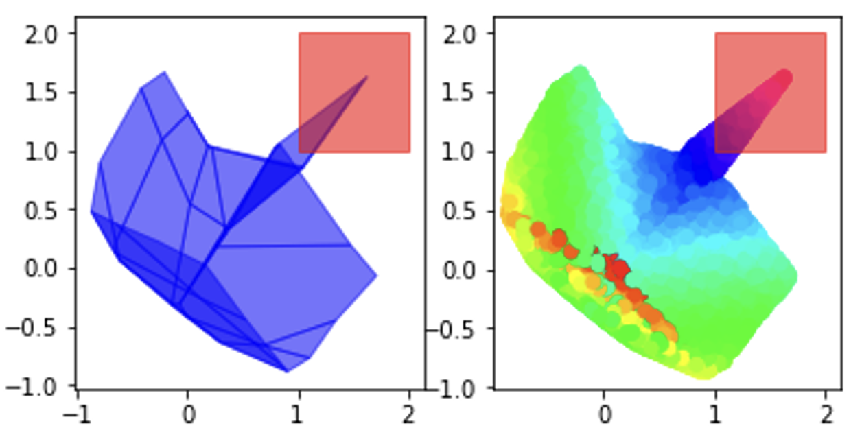
Figure 3: Unconstrained training, with $X^{(0pt)}$ plotted on the left and each $\mathbf{n}\!\left(\mathbf{x}^{(0)}_{j}\right)$ plotted on the right. The output approximates the function well but does not avoid the unsafe space.

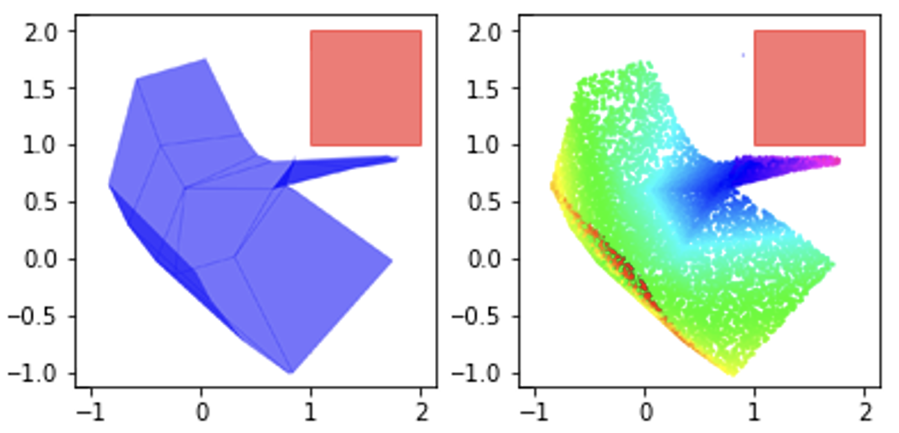
Figure 4: Constrained training. The output approximates the function while avoiding the unsafe space.

	Unconstrained	Constrained
final objective loss	0.0039	0.0127
final constraint loss	0.0575	0.0000

TABLE I:

V Conclusion and Future Work

This work proposes a constrained training method for feedforward ReLU neural networks. We demonstrated the method successfully on a small example of nonlinear function approximation. Given the ability to enforce output constraints, the technique can potentially be applied to offline training for safety-critical neural networks.

Our current implementation has several drawbacks to be addressed in future work. First, the method suffers an exponential blowup of constrained zonotopes through a ReLU. We hope to improve the forward pass step by using techniques such as [12] instead of layer-by-layer evaluation to compute the output set, and by conservatively estimating the reachable set similar to [13]. We also plan to apply the method on larger networks, such as for autonomous driving in [6] or the ACAS Xu network [26, 27, 28] for aircraft collision avoidance. In general, our goal is to train robust controllers where the output of a neural network must obey actuator limits and obstacle avoidance (for which the network output is passed through dynamics).

References

- [1] Guangming Xiong et al. “Development of assistant robot with standing-up devices for paraplegic patients and elderly people” In 2007 IEEE/ICME International Conference on Complex Medical Engineering, 2007, pp. 62–67 IEEE
- [2] ByungSoo Ko et al. “Neural network-based autonomous navigation for a homecare mobile robot” In 2017 IEEE International Conference on Big Data and Smart Computing (BigComp), 2017, pp. 403–406 IEEE
- [3] Guozheng Xu and Aiguo Song “Adaptive impedance control based on dynamic recurrent fuzzy neural network for upper-limb rehabilitation robot” In 2009 IEEE International Conference on Control and Automation, 2009, pp. 1376–1381 IEEE
- [4] Shahid Hussain, Sheng Q Xie and Prashant K Jamwal “Adaptive impedance control of a robotic orthosis for gait rehabilitation” In IEEE transactions on cybernetics 43.3 IEEE, 2013, pp. 1025–1034
- [5] Elena Gribovskaya, Abderrahmane Kheddar and Aude Billard “Motion learning and adaptive impedance for robot control during physical interaction with humans” In 2011 IEEE International Conference on Robotics and Automation, 2011, pp. 4326–4332 IEEE
- [6] Hoang-Dung Tran et al. “NNV: The neural network verification tool for deep neural networks and learning-enabled cyber-physical systems” In International Conference on Computer Aided Verification, 2020, pp. 3–17 Springer
- [7] LI Shengbo et al. “Key technique of deep neural network and its applications in autonomous driving” In Journal of Automotive Safety and Energy 10.2, 2019, pp. 119
- [8] Changliu Liu et al. “Algorithms for verifying deep neural networks” In arXiv preprint arXiv:1903.06758, 2019
- [9] Hoang-Dung Tran et al. “Star-based reachability analysis of deep neural networks” In International Symposium on Formal Methods, 2019, pp. 670–686 Springer
- [10] Hoang-Dung Tran, Stanley Bak, Weiming Xiang and Taylor T Johnson “Verification of deep convolutional neural networks using imagestars” In International Conference on Computer Aided Verification, 2020, pp. 18–42 Springer
- [11] Matthias Althoff “Reachability analysis and its application to the safety assessment of autonomous cars”, 2010
- [12] Joseph A Vincent and Mac Schwager “Reachable Polyhedral Marching (RPM): A Safety Verification Algorithm for Robotic Systems with Deep Neural Network Components” In arXiv preprint arXiv:2011.11609, 2020
- [13] Vicenc Rubies-Royo, Roberto Calandra, Dusan M Stipanovic and Claire Tomlin “Fast neural network verification via shadow prices” In arXiv preprint arXiv:1902.07247, 2019
- [14] Zhiheng Huang, Wei Xu and Kai Yu “Bidirectional LSTM-CRF models for sequence tagging” In arXiv preprint arXiv:1508.01991, 2015
- [15] Russell Stewart and Stefano Ermon “Label-free supervision of neural networks with physics and domain knowledge” In Proceedings of the AAAI Conference on Artificial Intelligence 31.1, 2017
- [16] Jingyi Xu et al. “A semantic loss function for deep learning with symbolic knowledge” In International Conference on Machine Learning, 2018, pp. 5502–5511 PMLR
- [17] Ulices Santa Cruz, James Ferlez and Yasser Shoukry “Safe-by-Repair: A Convex Optimization Approach for Repairing Unsafe Two-Level Lattice Neural Network Controllers” In arXiv preprint arXiv:2104.02788, 2021
- [18] Lukas Markolf and Olaf Stursberg “Polytopic Input Constraints in Learning-Based Optimal Control Using Neural Networks” In arXiv preprint arXiv:2105.03376, 2021
- [19] Joseph K Scott, Davide M Raimondo, Giuseppe Roberto Marseglia and Richard D Braatz “Constrained zonotopes: A new tool for set-based estimation and fault detection” In Automatica 69 Elsevier, 2016, pp. 126–136
- [20] Vignesh Raghuraman and Justin P Koeln “Set operations and order reductions for constrained zonotopes” In arXiv preprint arXiv:2009.06039, 2020
- [21] Jorge Nocedal and Stephen Wright “Numerical optimization” Springer Science & Business Media, 2006
- [22] Brandon Amos and J Zico Kolter “Optnet: Differentiable optimization as a layer in neural networks” In International Conference on Machine Learning, 2017, pp. 136–145 PMLR
- [23] Akshay Agrawal et al. “Differentiable convex optimization layers” In arXiv preprint arXiv:1910.12430, 2019
- [24] Boris Hanin and David Rolnick “Deep relu networks have surprisingly few activation patterns” In arXiv preprint arXiv:1906.00904, 2019
- [25] Adam Paszke et al. “Pytorch: An imperative style, high-performance deep learning library” In arXiv preprint arXiv:1912.01703, 2019
- [26] Mykel J Kochenderfer and JP Chryssanthacopoulos “Robust airborne collision avoidance through dynamic programming” In Massachusetts Institute of Technology, Lincoln Laboratory, Project Report ATC-371 130 Citeseer, 2011
- [27] Mykel J Kochenderfer, Jessica E Holland and James P Chryssanthacopoulos “Next-generation airborne collision avoidance system”, 2012
- [28] Mykel J Kochenderfer et al. “Optimized airborne collision avoidance” In Decision Making under Uncertainty, 2015, pp. 251