CutDepth:
Edge-aware Data Augmentation in Depth Estimation

Abstract

It is difficult to collect data on a large scale in a monocular depth estimation because the task requires the simultaneous acquisition of RGB images and depths. Data augmentation is thus important to this task. However, there has been little research on data augmentation for tasks such as monocular depth estimation, where the transformation is performed pixel by pixel. In this paper, we propose a data augmentation method, called CutDepth. In CutDepth, part of the depth is pasted onto an input image during training. The method extends variations data without destroying edge features. Experiments objectively and subjectively show that the proposed method outperforms conventional methods of data augmentation. The estimation accuracy is improved with CutDepth even though there are few training data at long distances.

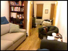
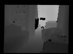
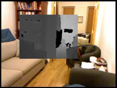
(a) Input image	(b) Depth	(c) Proposed method
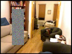
(d) CutOut	(e) RE	(f) CutMix

Figure 1: Examples of data augmentation

1 Introduction

Data augmentation is a practical way of improving the recognition performance without increasing the computational cost of inference. Various data augmentation methods have been proposed in the field of computer vision [1, 3, 5, 13, 14]. These data augmentation methods have been studied for higher-order tasks (e.g., object recognition). However, there has been little research on lower-order tasks, such as pixel-by-pixel transformations (e.g., monocular depth estimation).

The monocular depth estimation [7, 10] estimates depth from a single-view RGB image. This task requires the simultaneous acquisition of RGB images and depths. Data augmentation is required because it is difficult to collect a large amount of data. Image flipping, random cropping, and color and luminance transformation are often used for data augmentation. However, few studies have examined data augmentation that changes the geometry because such augmentation reduces the estimation accuracy.

Yoo et al. [12] proposed CutBlur, a data augmentation that adopts super-resolution. CutBlur improves the estimation accuracy by pasting a partial region of a high-resolution image onto the same position of a low-resolution image. The adoption of super-resolution generally has the problem of over-sharpening the estimated image. CutBlur, however, has a regularization effect, which prevents excessive sharpening and reduces the estimation error. Ghiasi et al. [2] proposed a data augmentation for segmentation in which images are cut and pasted in units of the instance.

We propose CutDepth, which is a data augmentation that pastes the area cut from the teacher data (depth) at the same position on the input image (RGB image). By replacing a part of the input image with depth, the change in appearance is greater than that in conventional data augmentations. Meanwhile, the change is small at the lower feature level because the edge positions of the depth and the RGB image are similar. CutDepth regularizes the image by depth because depth information is given to the input image. Therefore, the distance between the RGB image and the depth decreases in the latent space, and it becomes easier to estimate the depth.

The contributions of our work are as follows.

• We propose a new data augmentation method that both improves visual diversity and suppresses excessive geometric changes in the scene.

• We show the quality of the data distribution after data augmentation in terms of diversity and affinity.

• We show that the depth estimation performance is improved subjectively and objectively for a real image using the proposed data augmentation method.

2 Related work

2.1 Data augmentation

Optical transformations and geometric transformations can be conducted for data augmentation [8]. The former transformations include changing luminance and colors whereas the latter transformations include image flipping, translation, affine transformation, and random clipping.

There are methods of making changes optically and geometrically by replacing a partial area of the image with other information [1, 13, 14] (Figure 1). CutOut [1] and Random Erasing (RE) [14] replace a portion of the image with the average value of the image or a random number. CutMix [13] replaces a portion of an image with another image.

2.2 Monocular depth estimation

Monocular depth estimation [7, 10] is the task of estimating the depth from a single-viewpoint image. In monocular depth estimation, the input is an RGB image and the teacher data are of depth. BTS [7] has a structure that implicitly estimates the normal in a decoder. Monocular depth estimation has difficulty in estimating object contours. However, the BTS structure improves the accuracy of the contour estimation. Laplacian Depth [10] uses a Laplacian pyramid structure in a decoder. The structure uses the residuals obtained from the input image for each resolution. It effectively estimates both local details and the global layout.

3 Data augmentation for depth estimation

We propose a data augmentation called CutDepth (Figure 2). Let $x_{s}\in R^{W\times H\times C_{s}}$ be the input (RGB) image and $x_{t}\in R^{W\times H\times C_{t}}$ be the teacher (depth) data. $W$ and $H$ are, respectively, the width and height of the image and $C_{s}$ and $C_{t}$ are, respectively, the numbers of channels in the input image and the teacher data. $x^{\prime}_{s}$ with data augmentation on $x_{s}$ is obtained as

$$x^{\prime}_{s}=M*x_{s}+(1-M)*x_{t}.$$ (1)

If $C_{s}$ and $C_{t}$ are different, they are combined in the channel direction so that they are the same number in advance. $M$ is a matrix ($M\in\{0,1\}$) that indicates the region where $x_{s}$ is replaced by $x_{t}$. The position ($l$, $u$) and size ($w$, $h$) of the replacement region are obtained as

$$(l,u) = (a\times W,b\times H)$$ (2)

$$(w,h) = (\min((W-a\times W)\times c\times p,1),$$ (3)

$$\min((H-b\times H)\times d\times p,1)))$$ (4)

where $a$, $b$, $c$, and $d$ are $\mathcal{U}(0,1)$. $p$ is a hyperparameter that determines the maximum values of $w$ and $h$ for $W$ and $H$, and it is set at a value of $(0,1]$.

.

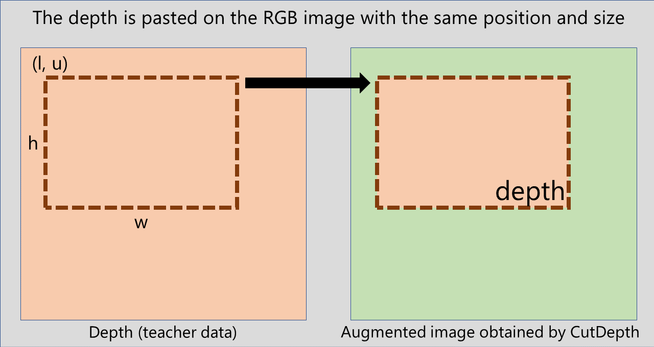
Figure 2: Data augmentation using CutDepth

Table 1: Comparison of the depth estimation performances when using different data augmentation methods. Lower Abs Rel, log10, RMSE and RMSE log indicate higher performance whereas higher d1, d2 and d3 indicate higher performance. The best performances are presented in bold text.

		BTS							Laplacian Depth
Method	p	Abs Rel $\downarrow$	log10 $\downarrow$	RMSE $\downarrow$	RMSE log $\downarrow$	d1 $\uparrow$	d2 $\uparrow$	d3 $\uparrow$	Abs Rel $\downarrow$	log10 $\downarrow$	RMSE $\downarrow$	RMSE log $\downarrow$	d1 $\uparrow$	d2 $\uparrow$	d3 $\uparrow$
Baseline		0.1122	0.048	0.406	0.145	0.878	0.979	0.995	0.11	0.047	0.39	0.139	0.884	0.983	0.996
CutOut	0.25	0.1122	0.048	0.405	0.144	0.878	0.98	0.996	0.106	0.046	0.384	0.136	0.891	0.984	0.996
	0.50	0.1118	0.048	0.402	0.144	0.879	0.981	0.996	0.109	0.046	0.382	0.137	0.889	0.983	0.997
	0.75	0.1146	0.05	0.414	0.148	0.871	0.979	0.996	0.106	0.045	0.382	0.135	0.893	0.985	0.997
	1.00	0.1194	0.051	0.427	0.152	0.864	0.977	0.996	0.11	0.047	0.394	0.14	0.884	0.984	0.997
Random	0.25	0.1106	0.048	0.4	0.143	0.88	0.981	0.996	0.109	0.046	0.384	0.137	0.89	0.982	0.996
Erasing	0.50	0.1116	0.048	0.4	0.143	0.881	0.981	0.996	0.106	0.045	0.378	0.134	0.892	0.985	0.997
	0.75	0.1132	0.049	0.415	0.147	0.871	0.979	0.996	0.106	0.045	0.379	0.134	0.893	0.985	0.997
	1.00	0.1186	0.051	0.429	0.152	0.863	0.977	0.996	0.111	0.047	0.394	0.14	0.884	0.983	0.997
CutMix	0.25	0.1105	0.047	0.397	0.142	0.882	0.981	0.996	0.107	0.046	0.388	0.137	0.889	0.983	0.996
	0.50	0.1132	0.049	0.406	0.146	0.874	0.979	0.996	0.107	0.046	0.386	0.136	0.891	0.983	0.996
	0.75	0.1231	0.054	0.438	0.158	0.848	0.976	0.996	0.107	0.046	0.386	0.136	0.891	0.983	0.996
	1.00	0.1851	0.086	0.674	0.241	0.659	0.918	0.982	0.11	0.047	0.391	0.139	0.886	0.982	0.996
Proposed	0.25	0.1083	0.047	0.398	0.141	0.884	0.981	0.996	0.106	0.045	0.38	0.135	0.895	0.984	0.996
	0.50	0.1077	0.046	0.391	0.14	0.884	0.982	0.997	0.104	0.044	0.375	0.132	0.899	0.985	0.997
	0.75	0.1074	0.047	0.392	0.14	0.885	0.982	0.996	0.106	0.045	0.379	0.135	0.894	0.984	0.997
	1.00	0.1127	0.047	0.392	0.142	0.88	0.981	0.996	0.104	0.045	0.376	0.132	0.898	0.985	0.996

Table 2: Comparison of the depth estimation performances when using different numbers of data ($p$ = 0.75). Lower Abs Rel, log10, RMSE and RMSE log indicate higher performance whereas higher d1, d2 and d3 indicate higher performance.

Scale	Method	Abs Rel $\downarrow$	log10 $\downarrow$	RMSE $\downarrow$	RMSE log $\downarrow$	d1 $\uparrow$	d2 $\uparrow$	d3 $\uparrow$
25%	Baseline	0.1226	0.052	0.428	0.154	0.859	0.977	0.995
	CutOut	0.1242	0.053	0.432	0.156	0.854	0.976	0.996
	RE	0.1268	0.054	0.440	0.158	0.848	0.976	0.995
	CutMix	0.1467	0.064	0.520	0.188	0.782	0.956	0.993
	Proposed	0.1225	0.052	0.424	0.153	0.858	0.978	0.995
50%	Baseline	0.1174	0.050	0.414	0.150	0.867	0.978	0.995
	CutOut	0.1168	0.050	0.418	0.150	0.867	0.979	0.996
	RE	0.1184	0.051	0.422	0.151	0.862	0.978	0.996
	CutMix	0.1307	0.056	0.460	0.168	0.832	0.970	0.994
	Proposed	0.1155	0.049	0.411	0.148	0.870	0.981	0.996
75%	Baseline	0.1154	0.049	0.410	0.147	0.871	0.979	0.996
	CutOut	0.1148	0.050	0.413	0.147	0.870	0.980	0.997
	RE	0.1179	0.051	0.424	0.151	0.863	0.977	0.996
	CutMix	0.1353	0.058	0.465	0.172	0.826	0.967	0.993
	Proposed	0.1142	0.048	0.401	0.144	0.876	0.981	0.996

4 Experimental results

4.1 Experimental setting

We use BTS [7] and Laplacian Depth [10] to evaluate the performance of the depth estimation. The optimizers are Adam and AdamW respectively. The learning rate is $10^{-4}$ for both, and the scheduling is performed with a polynomial decay (power of 0.9 and 0.5, respectively). The encoders are DenseNet161 [6] and ResNext-101 [11], pre-trained on ImageNet. The baseline data augmentation method uses horizontal flipping, color transformations, and image rotation randomly.

We use the NYU Depth V2 Dataset [9]. The image size used for training is 416 $\times$ 544 and that used for testing is 480 $\times$ 640, as in BTS [7]. As in BTS, 24,231 RGB image/depth pairs are used for training and 654 images are used for evaluation.

4.2 Depth estimation results

In addition to the baseline method, we use CutOut [1], RE [14], and CutMix [13]. Table 1 gives the evaluation results. The proposed method outperforms the conventional methods on all metrics. The depth estimation performance of the proposed method tended to be higher when $p$ was 0.5 or 0.75. The performances of the conventional methods decreased as $p$ increased. The performance of the proposed method did not degrade with increasing $p$ owing to the small change in the lower-order feature levels.

We next compare the depth estimation performances when the number of data are 25 %, 50 %, and 75 % of the original number and $p$ is set at 0.75. We randomly sample the data from the original dataset. Table 2 gives the evaluation results for different sizes of data. Even if the data size was small, the proposed method outperformed the other methods on various measures.

Figure 3 shows example results of depth estimation. Near distances are represented in blue and far distances in red. The proposed method outperformed the conventional methods in terms of the accuracy of the estimation for far distances and object contours. The conventional training model readily overfit some data because there were few data at a distance. However, the proposed method had better accuracy of the data at a distance because overfitting was reduced by regularization.

4.3 Evaluation of the effect of regularization

The distance between the RGB image and depth in the latent space becomes small if the image is regularized by depth. Therefore, to verify the regularization effect, we compare the distances in the latent space, which are the output of the BTS encoder, when the RGB image and depth are input to the BTS model. The root-mean-square error (RMSE), mean absolute error (MAE), and cosine distance are used as distance measures. Table 3 gives the comparison results. In terms of the RMSE and MAE, the distances of the proposed method and CutMix are comparable. However, the cosine distance is small for the proposed method. It is difficult to see the difference between the RMSE and MAE because of the small scale of the feature map. However, the difference becomes clear for the cosine distance where the scale is normalized.

4.4 Evaluation of the properties of data augmentation

We examine the properties of data augmentation. Gontijo-Lopes et al. [4] proposed the measurement of the properties of data augmentation in terms of diversity and affinity. A larger value of diversity corresponds to a greater spread of the data distribution due to data augmentation. A larger value of affinity corresponds to a smaller deviation from the original data distribution. Figure 4 plots the diversity and affinity of each method. Pink circles show the results of the proposed method and are encircled by a red dotted ellipse for clarity. Both the diversity and affinity of the proposed method are greater than those of the baseline method, and the distribution is thus more spread out and the deviation is smaller than for the original data. The proposed method has lower diversity than the various conventional methods, and the effect of suppressing excessive changes in edge features is thus confirmed.

BTS
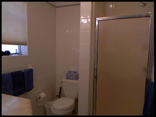
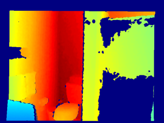
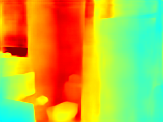
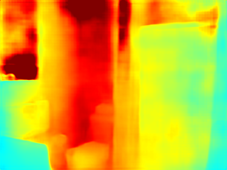
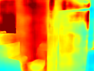
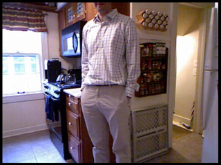
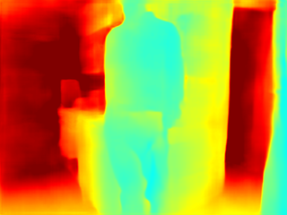
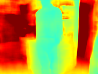
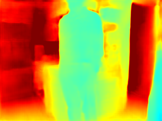
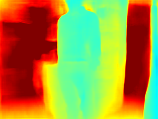
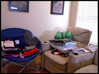
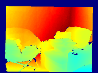
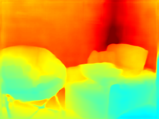
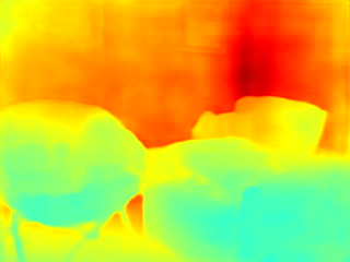
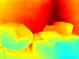
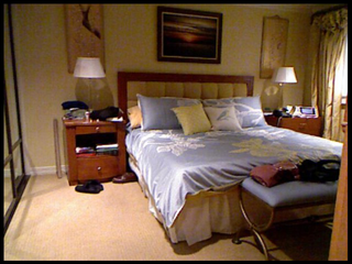
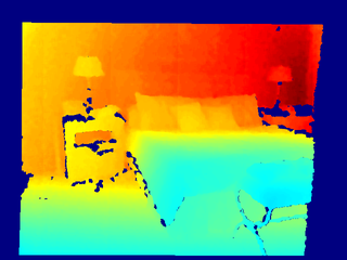
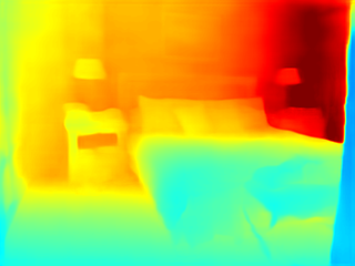
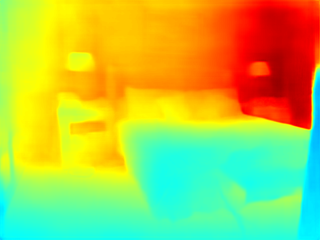
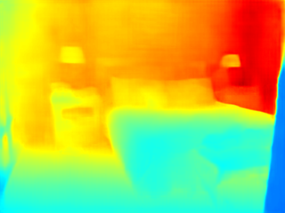
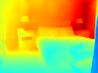
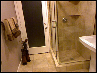
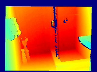
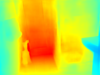
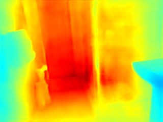
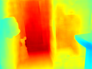
laplacian depth
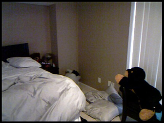
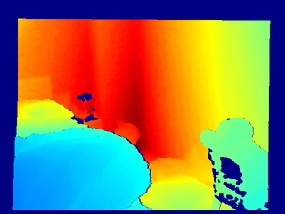
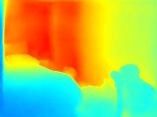
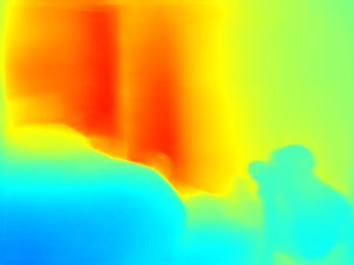
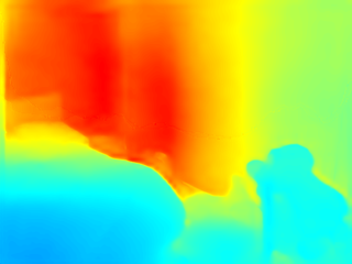
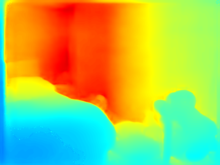
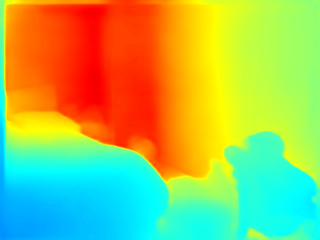
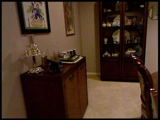
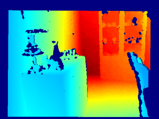
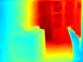
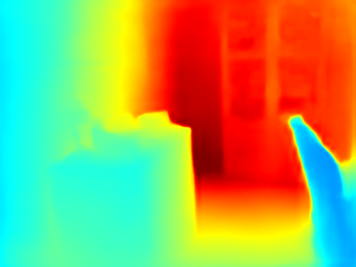
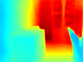
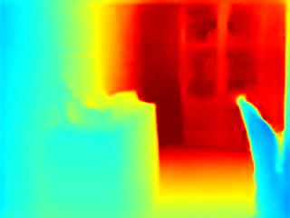
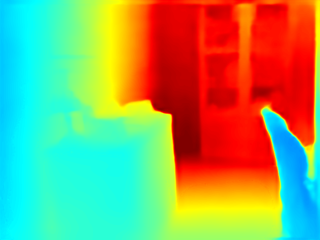
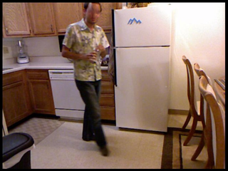
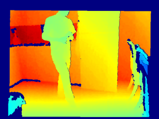
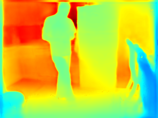
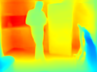
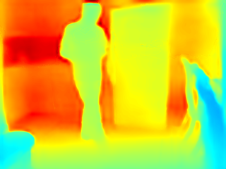
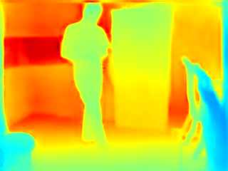
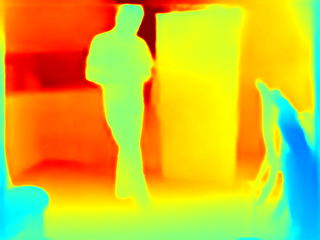
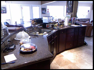
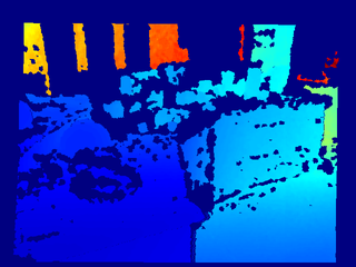
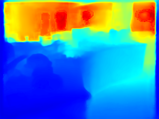
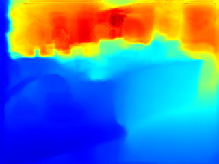
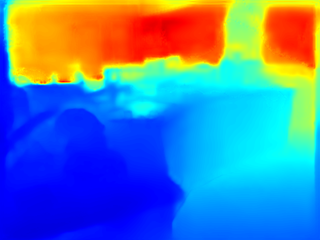
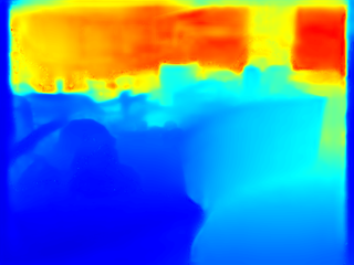
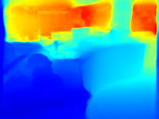
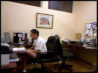
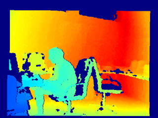
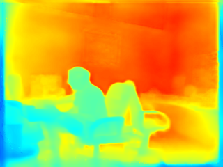
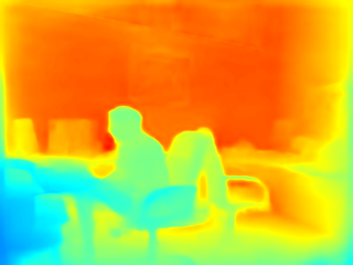
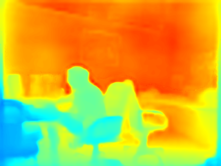
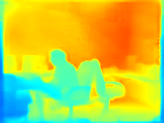
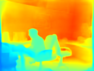
(a) RGB image	(b) Ground Truth	(c) Baseline	(d) CutMix	(e) CutOut	(f) RE	(g) Proposed

Figure 3: Depth estimation results obtained using different data augmentation methods

Table 3: Comparison of the distances between the RGB image and depth in the latent space

	p	RMSE $\downarrow$	MAE $\downarrow$	Cosine $\uparrow$
Baseline		1.094	0.49	0.24
CutOut	0.25	1.12	0.50	0.21
	0.50	1.16	0.52	0.17
	0.75	1.20	0.52	0.17
	1.00	1.39	0.61	0.15
Random	0.25	1.05	0.48	0.22
Erasing	0.50	1.09	0.49	0.20
	0.75	1.13	0.50	0.17
	1.00	1.17	0.52	0.17
CutMix	0.25	1.03	0.47	0.28
	0.50	0.92	0.41	0.22
	0.75	0.95	0.43	0.20
	1.00	1.35	0.50	0.12
Proposed	0.25	0.92	0.42	0.37
	0.50	1.06	0.48	0.37
	0.75	0.96	0.44	0.35
	1.00	1.07	0.48	0.33

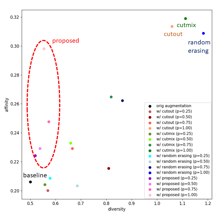
Figure 4: Comparison of diversity and affinity between different data augmentation methods

5 Conclusion

We proposed a data augmentation method, called CutDepth, for depth estimation. CutDepth is a method of pasting part of the depth to an input image, which increases the variation of the input image. We confirmed that the estimation accuracy of the proposed method is better than that of conventional methods. In the proposed method, the edge features are similar before and after the data augmentation. We therefore found that the proposed method does not expand the data distribution excessively compared with the conventional methods. In future work, we will test the effectiveness of the proposed method in tasks other than depth estimation.

References

- [1] Terrance DeVries and Graham W Taylor. Improved regularization of convolutional neural networks with cutout. arXiv preprint arXiv:1708.04552, 2017.
- [2] Golnaz Ghiasi, Yin Cui, Aravind Srinivas, Rui Qian, Tsung-Yi Lin, Ekin D Cubuk, Quoc V Le, and Barret Zoph. Simple copy-paste is a strong data augmentation method for instance segmentation. arXiv preprint arXiv:2012.07177, 2020.
- [3] Chengyue Gong, Dilin Wang, Meng Li, Vikas Chandra, and Qiang Liu. Keepaugment: A simple information-preserving data augmentation approach. arXiv preprint arXiv:2011.11778, 2020.
- [4] Raphael Gontijo-Lopes, Sylvia J Smullin, Ekin D Cubuk, and Ethan Dyer. Affinity and diversity: Quantifying mechanisms of data augmentation. arXiv preprint arXiv:2002.08973, 2020.
- [5] Dan Hendrycks and Thomas Dietterich. Benchmarking neural network robustness to common corruptions and perturbations. arXiv preprint arXiv:1903.12261, 2019.
- [6] Gao Huang, Zhuang Liu, Laurens Van Der Maaten, and Kilian Q Weinberger. Densely connected convolutional networks. In Proceedings of the IEEE conference on computer vision and pattern recognition, pages 4700–4708, 2017.
- [7] Jin Han Lee, Myung-Kyu Han, Dong Wook Ko, and Il Hong Suh. From big to small: Multi-scale local planar guidance for monocular depth estimation. arXiv preprint arXiv:1907.10326, 2019.
- [8] Connor Shorten and Taghi M Khoshgoftaar. A survey on image data augmentation for deep learning. Journal of Big Data, 6(1):1–48, 2019.
- [9] Nathan Silberman, Derek Hoiem, Pushmeet Kohli, and Rob Fergus. Indoor segmentation and support inference from rgbd images. In European conference on computer vision, pages 746–760. Springer, 2012.
- [10] Minsoo Song, Seokjae Lim, and Wonjun Kim. Monocular depth estimation using laplacian pyramid-based depth residuals. IEEE Transactions on Circuits and Systems for Video Technology, 2021.
- [11] Saining Xie, Ross Girshick, Piotr Dollár, Zhuowen Tu, and Kaiming He. Aggregated residual transformations for deep neural networks. In Proceedings of the IEEE conference on computer vision and pattern recognition, pages 1492–1500, 2017.
- [12] Jaejun Yoo, Namhyuk Ahn, and Kyung-Ah Sohn. Rethinking data augmentation for image super-resolution: A comprehensive analysis and a new strategy. In Proceedings of the IEEE/CVF Conference on Computer Vision and Pattern Recognition, pages 8375–8384, 2020.
- [13] Sangdoo Yun, Dongyoon Han, Seong Joon Oh, Sanghyuk Chun, Junsuk Choe, and Youngjoon Yoo. Cutmix: Regularization strategy to train strong classifiers with localizable features. In Proceedings of the IEEE/CVF International Conference on Computer Vision, pages 6023–6032, 2019.
- [14] Zhun Zhong, Liang Zheng, Guoliang Kang, Shaozi Li, and Yi Yang. Random erasing data augmentation. In Proceedings of the AAAI Conference on Artificial Intelligence, pages 13001–13008, 2020.