Considerations for optimizing photometric classification of supernovae from the Rubin Observatory

Abstract

The Vera C. Rubin Observatory will increase the number of observed supernovae (SNe) by an order of magnitude; however, it is impossible to spectroscopically confirm the class for all the SNe discovered. Thus, photometric classification is crucial but its accuracy depends on the not-yet-finalized observing strategy of Rubin Observatory’s Legacy Survey of Space and Time (LSST). We quantitatively analyze the impact of the LSST observing strategy on SNe classification using simulated multi-band light curves from the Photometric LSST Astronomical Time-Series Classification Challenge (PLAsTiCC). First, we augment the simulated training set to be representative of the photometric redshift distribution per supernovae class, the cadence of observations, and the flux uncertainty distribution of the test set. Then we build a classifier using the photometric transient classification library snmachine, based on wavelet features obtained from Gaussian process fits, yielding similar performance to the winning PLAsTiCC entry. We study the classification performance for SNe with different properties within a single simulated observing strategy. We find that season length is important, with light curves of $150$ days yielding the highest performance. Cadence also has an important impact on SNe classification; events with median inter-night gap $<3.5$ days yield higher classification performance. Interestingly, we find that large gaps ($>10$ days) in light curve observations do not impact performance if sufficient observations are available on either side, due to the effectiveness of the Gaussian process interpolation. This analysis is the first exploration of the impact of observing strategy on photometric supernova classification with LSST.

1 Introduction

The upcoming Rubin Observatory Legacy Survey of Space and Time (LSST) (LSST Science Collaboration et al., 2009, 2017; Ivezić et al., 2019) is expected to discover, during its ten-year duration, at least one order of magnitude more supernovae (SNe) than the current available SNe samples (Guillochon et al., 2017). Traditionally, SNe that are used in astrophysical and cosmological studies need to be spectroscopically classified (e.g. Riess et al., 1998; Astier et al., 2006; Kessler et al., 2009). However, this will be impossible for most events detected by LSST due to the limited spectroscopic resources; thus, LSST will rely on photometric classification, using the events that will be spectroscopically classified as its training set.

Previous efforts to understand the strengths and limitations of photometric classification algorithms resulted in the Supernova Photometric Classification Challenge (SNPhotCC; Kessler et al., 2010a) in preparation for the Dark Energy Survey (DES; The Dark Energy Survey Collaboration & Flaugher, 2005). Recently, the Photometric LSST Astronomical Time-Series Classification Challenge (PLAsTiCC; The PLAsTiCC team et al., 2018; Kessler et al., 2019) was launched in preparation for LSST, which will reach fainter magnitudes and have a $\sim 4$ times larger survey area compared to DES. The classifiers applied to the datasets from these challenges employed parametric fits, template fits, and machine learning models such as neural networks, boosted decision trees, support vector machine, and gradient boosting (e.g. Kessler et al., 2010b; Lochner et al., 2016; Charnock & Moss, 2017; Pasquet et al., 2019; Muthukrishna et al., 2019; Villar et al., 2020).

To obtain accurate classification, the training set must be representative of the test set (e.g. Lochner et al. 2016). However, photometric classifiers are typically trained with non-representative spectroscopically-confirmed events that are biased towards lower redshifts. Thus, recent work has focused on overcoming the lack of representativeness (Muthukrishna et al., 2019; Pasquet et al., 2019; Revsbech et al., 2017; Boone, 2019; Carrick et al., 2021). Photometric classification performance also depends on the survey observing strategy; however, this dependence has not yet been explored.

The LSST observing strategy encompasses diverse considerations such as season length, survey footprint, single visit exposure time, inter-night gaps, and cadence of repeat visits in different passbands. The observing strategy is currently being optimized (LSST Science Collaboration et al., 2017; Ivezić et al., 2018; Lochner et al., 2018; Gonzalez et al., 2018; Laine et al., 2018; Jones et al., 2020), a challenging task since the survey has diverse goals (LSST Science Collaboration et al., 2009; Ivezić et al., 2019). Recently, the Rubin Observatory LSST Dark Energy Science Collaboration (DESC) Observing Strategy Working Group investigated the impact of observing strategy on cosmology and made recommendations for its optimization (Scolnic et al., 2018; Lochner et al., 2018, 2021). In particular, SNe cosmology requires a high and regular cadence with long season lengths (how long a field is observable in a year).

In this work, we upgrade the photometric transient classification library snmachine (Lochner et al., 2016) for use with LSST data and build a classifier based on wavelet features obtained from Gaussian process (GP) fits. We also include the host-galaxy photometric redshifts and their uncertainties as features. We make several other improvements to deal with the greater realism of the PLAsTiCC data, including training set augmentation. Using this improved classifier we study the performance of photometric SNe classification for subsets of light curves with different cadence properties, using the single observing strategy simulated for the PLAsTiCC challenge. We note that this approach is different from studying the classification performance for different observing strategies with fixed total exposure time, where a reduced season length could be compensated by a higher cadence.

In Sections 2 and 3 we summarize the PLAsTiCC dataset and describe the classification pipeline, respectively. Section 4 focuses on the augmentation methodology. Our results and their implications for observing strategy are described in Section 5. We conclude in Section 6.

2 PLAsTiCC Dataset

The PLAsTiCC (The PLAsTiCC team et al., 2018; PLAsTiCC Team & PLAsTiCC Modelers, 2019) dataset consists of simulations of $18$ different classes of transients and variable stars. It contains three-year-long light curves of $3.5$ millions events observed in the LSST $ugrizy$ passbands, as well as their host-galaxy photometric redshifts and uncertainties. Although the simulations included realistic observing conditions, the observing strategy used is now outdated (Jones et al., 2020). PLAsTiCC mimicked future LSST observations in two survey modes: the Wide-Fast-Deep (WFD) survey, which covers almost half the sky and was used for $99\%$ of the events, and the Deep-Drilling-Fields (DDF) survey, small patches of the sky with more frequent and deeper observations that have smaller flux uncertainties.

The simulations were divided into a non-representative spectroscopically-confirmed training set biased towards brighter events, and which is $0.2\%$ of the size of the test set. The training set was much smaller, to mimic the data that will be available at the start of LSST science operations from current and near-term spectroscopic surveys. In particular, the training set was loosely modeled on the magnitude-limited 4-metre Multi-Object Spectroscopic Telescope Time Domain Extragalactic Survey (Swann et al., 2019), resulting in a sample with a mean redshift $\sim 0.3$. The unblinded dataset is available in PLAsTiCC Team & PLAsTiCC Modelers (2019), the model libraries are presented in PLAsTiCC Modelers (2019), and more details about the models and simulations, including the description of the training set, host-galaxy photometric redshifts and their uncertainties, are given in Kessler et al. (2019). In this work we provide observing strategy recommendations to improve photometric classification of SNe in particular, so we restrict ourselves to the PLAsTiCC classes SN Ia, SN Ibc, and SN II; Table 1 shows a breakdown of the numbers of SNe in each class.

3 Classification pipeline

In this section we describe how we upgraded the photometric classification pipeline snmachine for use with PLAsTiCC data. Augmentation was a crucial step in this process, and it is discussed in greater detail in Section 4.

3.1 Light Curve Preprocessing

PLAsTiCC light curves have long gaps ($>50$ days) in the observations because any given sky location is not visible from the Vera C. Rubin Observatory site for several months of the year. Additionally, the SNe are only detected for a few months so including the entire three-year-long light curve provides irrelevant information to the classifier, which in turn degrades its performance. In order to isolate the observing season that contains the SNe, we selected the season which contains the observations flagged as detected, and which has no inter-night gaps larger than $50$ days. To introduce uniformity in the dataset, we translated the resulting light curves so their first observation is at time zero. However, this results in light curves that peak at different times, so we explored additionally shifting all training set light curves randomly in time to capture a larger variability of peak times. We found that augmenting with this random shift led to a less representative training set, and thus to a worse classification performance. Therefore, in this work, we simply aligned the first observation of the training events at time zero, such as we did for the test set. Figure 1 shows an example of light curve preprocessing.

Table 1: Breakdown of the number of SNe per class used in this work (see simulation details in Kessler et al. (2019)). For each class, the number of events in the training and test set is shown.

SN class	$N_{\mathrm{training}}$ (%)	$N_{\mathrm{test}}$ (%)
SN Ia	$2\,313$ ($58\%$)	$1\,659\,831$ ($59\%$)
SN Ibc	$484$ ($12\%$)	$175\,094$ ($6\%$)
SN II	$1\,193$ ($30\%$)	$1\,000\,150$ ($35\%$)
Total	$3\,990$ ($100\%$)	$2\,835\,075$ ($100\%$)

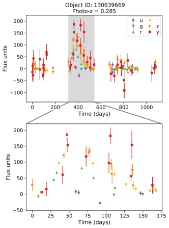
Figure 1: Example of a simulated LSST type Ibc supernova light curve from PLAsTiCC, showing how we preprocess light curves to remove season gaps. The original and processed light curves are shown in the top and bottom panels, respectively. The processed light curve corresponds to the shaded region on the original light curve with the first observation translated to time zero. The observations in different passbands are shown in different colors.

3.2 Gaussian Process Modeling of Light Curves

We modeled each light curve with a GP regression (e.g. MacKay, 2003; Rasmussen & Williams, 2005), following previous works that successfully used GP-modeled light curves in their classification pipelines (e.g. Lochner et al., 2016; Revsbech et al., 2017). Unlike the previous examples that fitted separate GPs to each passband, Boone (2019) fitted GPs both in time and wavelength, thus allowing the GPs to incorporate cross-band information. Figure 2 shows that such a two-dimensional GP fit infers the SNe light curve even in passbands where there are none or only a few observations, in contrast to the one-dimensional GP fit. Thus, we used two-dimensional GPs to fit light curves both in time and wavelength.

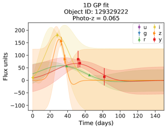
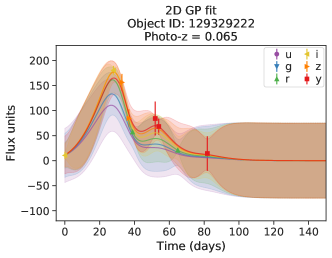
Figure 2: SN Ibc light curve, where the points show the observations, along with their errorbars, and the lines and the shaded regions show the mean and standard deviation of the GP fit, respectively. The left panel shows the one-dimensional GP fit to each available passband and the right panel shows the two-dimensional GP fit to all the passbands (shown in different colors). The two-dimensional GP infers the light curve in passbands where there are no (or few) observations, unlike the one-dimensional GP.

We chose a null mean function for the GP, modeling the events as perturbations to a flat background. Following Boone (2019), we used the once-differentiable Matérn 3/2 kernel for the GP covariance, which is appropriate for modeling explosive transients with sudden changes in their flux. The time dimension length-scale and amplitude were optimized per event, using maximum likelihood estimation. We fixed the length-scale of the wavelength dimension to $6000\,\mathring{\mathrm{A}}$ as in Boone (2019), since they found that this value produces reasonable models for all classes in PLAsTiCC. The GPs were implemented with the package George (Ambikasaran et al., 2014).

3.3 Feature Extraction

In this work we followed the wavelet decomposition approach of Lochner et al. (2016) to extract features. Since this is a model-independent approach to feature extraction, it does not assume any physical knowledge about the observed phenomena; hence it is applicable to any time-series data. Moreover, recent results showed wavelet decomposition was successful for general transient classification (Varughese et al., 2015; Lochner et al., 2016; Sooknunan et al., 2021; Narayan et al., 2018). This model-independent approach had not been used previously by the winning PLAsTiCC entries.

Following Lochner et al. (2016), we used a Stationary Wavelet Transform and the symlet family of wavelets; the wavelet decomposition was implemented with the package PyWavelets (Lee et al., 2019a). To obtain the wavelet decomposition, we first used the GPs to interpolate all light curves onto the same time grid of $277$ days (maximum light curve length of the events); we chose approximately one grid point per day and used a two-level wavelet decomposition, following Lochner et al. (2016). These choices resulted in $6624$ (highly redundant) wavelet coefficients per event. While it is common to combine GP fits and wavelet analysis (e.g. Chen et al., 2013; Istas, 1992; Pope, 2019, and references therein), we note that our method of modeling the sparse light curves with GP fits and then using wavelet decomposition to obtain classification features is unusual. This approach was briefly mentioned in Varughese et al. (2015), and firstly implemented in Lochner et al. (2016).

Following Lochner et al. (2016), we reduced the dimensionality of this wavelet space using Principal Component Analysis (PCA) (Pearson, 1901; Hotelling, 1933) on the wavelet coefficients of the augmented training set. After comparing the classifier performance on a validation set (we set aside $5\%$ of the test set for validation) with different numbers of PCA components, we found that $20-50$ components were the best to distinguish different types of SNe (their log-loss differs by around $2\%$); we chose $40$ components ($99.995\%$ of the total variance) due to its slightly better performance.

Finally, we also include the photometric redshift and its uncertainty as classification features. Unlike our previous results on the SNPhotCC challenge (Lochner et al., 2016) we find that these features are crucial for solving the more realistic classification challenge presented by the PLAsTiCC data. This is also confirmed by other PLAsTiCC analyses (Boone, 2019; Hložek et al., 2020).

3.4 Classification

We augmented the training set as described in Section 4, prior to training a classifier. We used the Gradient Boosting Model implementation of the package LightGBM (Ke et al., 2017), in particular the Gradient Boosting Decision Tree (GBDT) (Friedman, 2001). These are ensemble classifiers that produce predictions using ensembles of decision trees. The boosting improves the ensemble prediction by sequentially adding new decision trees that prioritize difficult-to-classify events. Boosted decision trees are commonly used in machine learning pipelines, including most of the top solutions to PLAsTiCC challenge (Hložek et al., 2020), due to their robust predictions, capacity for handling missing data, and flexibility (Friedman, 2001; Ke et al., 2017).

We optimized the GBDT hyperparameters (parameters of the model that must be set before the learning process starts) by maximizing the performance of a $5$-fold cross-validated grid-search on the augmented training set. First, each hyperparameter was optimized individually using a one-dimensional grid, keeping the other hyperparameters at default values. Then, we constructed a six-dimensional grid with three possible values for each hyperparameter informed by the earlier one-dimensional optimization. Finally we optimized this six-dimensional grid through a standard grid search. The resulting hyperparameter values are shown in Table 2. Since training and testing on the same events leads to overfitting, we placed in the same cross-validation fold all synthetic events that were derived from the same original event. While alternative hyperparameter optimization techniques can be considered (e.g. Bayesian optimization; Mockus et al., 1978; Snoek et al., 2012), a simple grid search strategy as described above proved to be effective.

Table 2: Optimized hyperparameter values used for the LightGBM model. A description of the hyperparameters is given in the library documentation.

Hyperparameter	WFD setting	DDF setting
boosting_type	gbdt	gbdt
learning_rate	$0.24$	$0.24$
max_depth	$16$	$19$
min_child_samples	$25$	$70$
min_split_gain	$0.3$	$0.3$
n_estimators	$115$	$45$
num_leaves	$50$	$50$

3.4.1 Performance Evaluation

In order to evaluate the classification performance, we used the PLAsTiCC weighted log-loss metric (The PLAsTiCC team et al., 2018; Malz et al., 2019) given by

$$\text{Log-loss}=-\left(\dfrac{\sum_{i=1}^{M}w_{i}\cdot\sum_{j=1}^{N_{i}}\frac{y_{ij}^{*}}{N_{i}}\cdot\ln p_{ij}}{\sum_{i=1}^{M}w_{i}}\right)\,,$$ (1)

where $M$ is the total number of classes, $N_{i}$ is the number of events in class $i$, $y_{ij}^{*}$ is $1$ if observation $j$ belongs to type $i$ and $0$ otherwise, $p_{ij}$ is the predicted probability that event $j$ belongs to class $i$ and $w_{i}$ is the weight of the class $i$. The weights can be changed to give different importances to different classes; however, following the PLAsTiCC challenge, we gave the same weight to every SNe class.

We used confusion matrices to visualize the mislabeled classes; Table 3 shows the confusion matrix for a binary classification. For ease of comparison, we normalized the confusion matrices by dividing each entry by the true number of each SNe class; hence the identity matrix represents a perfect classification.

Table 3: Confusion matrix for binary classification.

		True class
		Positive (P)	Negative (N)
Predicted	P	True positive ($\mathrm{TP}$)	False positive ($\mathrm{FP}$)
class	N	False negative ($\mathrm{FN}$)	True negative ($\mathrm{TN}$)

For a single SNe class, it is also common to use the recall (also called completeness/sensitivity) to measure the fraction of correctly-classified SNe, and the precision to measure the fraction of SNe assigned to the considered class that are indeed from that class. These are defined as

$$\mathrm{recall}=\dfrac{\mathrm{TP}}{\mathrm{TP}+\mathrm{FN}}$$ (2)

and

$$\mathrm{precision}=\dfrac{\mathrm{TP}}{\mathrm{TP}+\mathrm{FP}}\,.$$ (3)

Redshift distribution per class

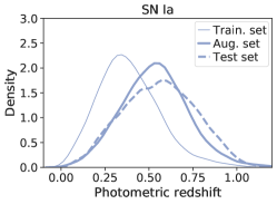
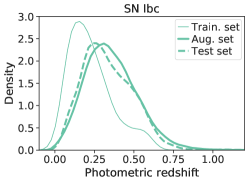
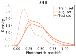
Figure 3: Host galaxy photometric redshift distribution per supernova class, where SN Ia, SN Ibc, SN II are shown, respectively, on the left, middle and right panels. The distribution of the training, augmented training and test sets are shown as fine solid, bold solid and dashed lines, respectively. Although the training set distribution is not representative of the test set, the augmented training set (Section 4) is close to the desired test distribution.

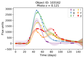
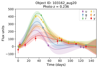
Figure 4: The left panel shows a SN Ibc light curve where the points show the observations, along with their errorbars, and the lines and the shaded regions show the mean and standard deviation of the GP fit, respectively. The right panel shows a synthetic event at a different redshift generated from the original event using the procedure described in Section 4. Note that, in this example, the original event was simulated in the higher-cadence DDF survey and we generated the synthetic event in the WFD survey.

4 Augmentation

As previously outlined, the PLAsTiCC training set is non-representative of the test set in redshift (see Figure 3) and also imbalanced: the most common SNe class has $\sim 4.8$ times more events than the least common. However, to obtain accurate classification the training set must be representative (Lochner et al., 2016) and balanced (as later discussed in Section 4.1).

Recent augmentation approaches rely on generating synthetic light curves from the GPs fitted to training set events (Revsbech et al., 2017; Boone, 2019). In particular, Boone (2019) simulated new sets of observations for each object such that they match the cadence, depth and uncertainty of observations of the test set, which ensured the representativity of these properties irrespective of the quality of the original event. The augmented observations were drawn from the mean prediction of the GP, and blocks of observations were dropped to simulate season boundaries. Additionally, Boone (2019) introduced redshift augmentation, where the observations of a new synthetic event are simulated at a different redshift from the original.

We adapted the approach used in Boone (2019) for our training set augmentation. Figure 4 shows a synthetic light curve generated using our augmentation procedure, which can be summarized as follows:

1. Choose the number of synthetic events to create (Section 4.1).

2. Model the original light curve with a two-dimensional GP fit in time and wavelength (as described in Section 3.2).

3. Choose a redshift for the synthetic event (Section 4.2).

4. Create synthetic observations at the new redshift, making use of the GP fit to the original event (Section 4.3).

5. Generate a photometric redshift (Section 4.4).

The WFD and DDF surveys have very different characteristics and enable qualitatively different science goals. Hence we found it is important to use customized augmentation for the two survey-modes, in contrast to the approach of the winning PLAsTiCC entries. Since the DDF survey has a different redshift distribution, higher cadence, and higher signal-to-noise ratio than the WFD survey, we must use a different augmentation and, consequently, a different classifier.

We now describe the augmentation procedure in detail. The reader should keep in mind, where relevant, that the augmentation procedure was customized for the two survey modes as necessary.

4.1 Number and Class Balance of Synthetic Events

As we wish to optimize classification performance for all SNe classes, we generated an augmented training set with the same number of events per class (i.e., a balanced training set). We also investigated an augmentation of the training set to resemble the class proportions of the test set ($\sim 59\%$ SN Ia, $\sim 6\%$ SN Ibc, $\sim 35\%$ SN II). However this gave worse performance, biasing the predictions toward the most common class.

We determined that the performance of the classifier stabilized when the size of the WFD augmented training set was around $4\times 10^{4}$. In this final configuration, each training set SN was augmented up to $140$ times. The DDF augmented training set stabilized around $8\times 10^{3}$, and each DDF training set SN was augmented up to $70$ times.

4.2 Redshift Augmentation

As previously outlined, redshift augmentation was found to be critical for the PLAsTiCC dataset (Boone, 2019). Figure 3 shows the bias of the training set towards low-redshift events in comparison to the test set. We augmented each training set event of the WFD survey between

$$\begin{aligned} z_{\mathrm{min}}&\approx\max\left\{0,0.90\,z_{\mathrm{ori}}-0.10\right\}\,\text{and}\\ z_{\mathrm{max}}&\approx 1.43\,z_{\mathrm{ori}}+0.43\,,\end{aligned}\,$$ (4)

where $z_{\mathrm{ori}}$ is the spectroscopic redshift of the original event. For the augmentation, we used a target distribution that is class-agnostic. First, we drew an auxiliary value $z^{*}$ from a log-triangular distribution with minimum value and mode $\log(z_{\mathrm{min}})$, and maximum value $\log(z_{\mathrm{max}})$. Then, we calculated the redshift of the new augmented event $z_{\mathrm{aug}}$,

$$z_{\mathrm{aug}}\left(z^{*}\right)=-z^{*}+z_{\mathrm{min}}+z_{\mathrm{max}}\,.$$ (5)

For the deeper DDF survey, the corresponding $z_{\mathrm{max}}$ was increased by $40\%$, otherwise the same procedure was followed. These limits arise due to the fact that for a given event in the original training set, its GP fit is more reliable close to the observations; hence we limit the GP extrapolation in wavelength when generating synthetic events, which translates into the above redshift constraint. This distribution differs slightly from Boone (2019), which also uses a class-agnostic augmentation. We derive the aforementioned redshift limits for augmentation in Appendix A.

The process of actually redshifting the light curve after choosing the new redshift is discussed below.

4.3 Generating Realistic Synthetic Observations

The first step in generating the synthetic light curves is selecting the epochs at which mock observations will be made. Our implementation proceeded as in Boone (2019); we summarize the approach as follows. First, we stretched the observed epochs of the original event to account for the time dilation due to the difference between the original and augmented redshifts. We also removed any observations that fell outside the observing window as a consequence. Then we randomly picked a target number of observations from a Gaussian mixture model based on the test set. However, this fails to account for the change in the cadence due to redshift augmentation; events shifted to higher redshifts have a lower density of observations than the events observed at those redshifts. In order to account for this, we multiplied this target number by $(1+z_{\mathrm{aug}})/(1+z_{\mathrm{ori}})$. We then generated additional observations at the same epochs as existing observations in randomly-selected passbands, associating each synthetic observation with an observed epoch in the original light curve. Further, to avoid creating synthetic light curves where most of the observations are obtained through this procedure, we capped the number of additional observations generated to be less than $50\%$ of the total number of observations in the original light curve. If this procedure resulted in more observations than the original target number drawn from the Gaussian mixture model, we then randomly dropped observations (original or new) until the target number was reached. Otherwise, to introduce additional variability, we randomly dropped $10\%$ of the synthetic observations.

Once we determined the epochs at which new observations would be generated, we redshifted the light curve as follows. We first computed the central wavelengths of the ugrizy passbands of the synthetic event as seen at the redshift of the original event. Then, we computed the mean and uncertainty of the GP fit to the original event, at the observed epochs of the original event associated with the synthetic observations but at the redshifted wavelengths. The steps so far dealt with the time dilation but not with the cosmological dimming of the synthetic event. Assuming a standard cosmological model, we redshifted the flux of the synthetic event and its uncertainty, such that it is observed at $z_{\mathrm{aug}}$. Further details of this redshifting implementation are given in Appendix A.

Following Boone (2019), we then combined the flux uncertainty of the augmented events predicted by the GP in quadrature with a value drawn from the flux uncertainty distribution of the test set, in order to achieve a more representative flux uncertainty distribution for the augmented training set. We also drew noise to add to the flux of the augmented events from a Gaussian with standard deviation of the aforementioned value from the flux uncertainty distribution.

Finally, we imposed quality cuts on the synthetic events in order to decide whether to add them to the augmented training set. To make the synthetic events as similar as possible to the test set events, we use a 2-detection trigger based on PLAsTiCC (Kessler et al., 2019). Boone (2019) fitted an error function to the observations from the full dataset to predict the probability of detection as a function of signal-to-noise ratio (S/N), and applied this probabilistic threshold to all observations. Boone (2019) then accepted an event if at least two of its observations were predicted as detected. However, we find that this was insufficient to constraining a GP, thus we required an additional observation, without requiring it to be predicted as detected by the chosen probabilistic detection threshold. Note that all synthetic light curves in the augmented DDF training set meet this quality cut as they are generated with a higher number of observations.

4.4 Photometric Redshift

In order to simulate realistic photometric redshifts for the synthetic events, following Boone (2019) we chose a random event from the $\sim 4\%$ of test set events that had a spectroscopic redshift measurement, and calculated the difference between its spectroscopic and photometric redshifts. We then added this difference to the true redshift of the augmented event to generate a photometric redshift.

4.5 Computational Resources

We performed our computations on an Intel(R) Xeon(R) CPU E5-2697 v2 (2.70GHz). Using a single core, the pipeline takes $\sim 1$ min to fit GPs to $1000$ events, and to perform their wavelet decomposition. Generating a balanced augmented training set with $4\times 10^{4}$ events takes $\sim 9$ hrs. Reducing the dimensionality using PCA takes $\sim 30$ min for an augmented training set of $4\times 10^{4}$ events and optimizing the LightGBM classifier on the same training set takes $\sim 8$ hrs. After we computed the test set features, generating predictions with the trained classifier takes $\sim 10$ min. Overall, the entire classification pipeline takes $\sim 70$ core hours of computing time for WFD and $12$ for DDF in this setting.

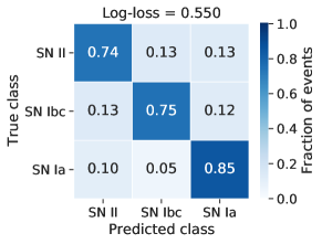
Figure 5: WFD test set normalized confusion matrix for the classifier trained on the augmented training set and its log loss performance. Each event is assigned to the class with the highest prediction.

5 Results and Implications for Observing Strategy

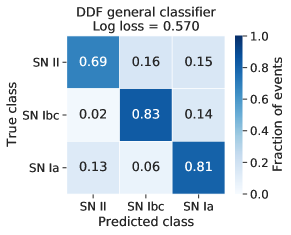
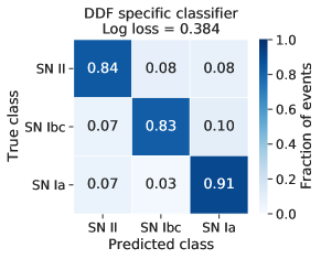
Figure 6: DDF test set normalized confusion matrix for the classifier trained with (left panel) the general WFD+DDF augmented training set and (right panel) with the DDF-only augmented training set. The results show the importance of using an augmented training set customized for the specific survey mode characteristics.

We now turn to our results on the PLAsTiCC dataset and consider in detail their implications for various aspects of the LSST observing strategy. We study classification performance for SNe with different properties within the single simulated observing strategy that is available in PLAsTiCC. We present results related to classification performance for the two different survey modes (WFD and DDF) in Section 5.1. We then explore the performance as a function of light curve length (Section 5.2), median inter-night gap (Section 5.3), number of gaps $>10$ days (Section 5.3), and number of observations near the peak (Section 5.4).

5.1 Survey Mode-specific Augmentation and its Effect on Performance

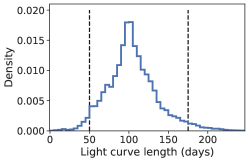
Figure 7: WFD test set recall (left panel) and precision (middle panel) as a function of light curve length per SNe class. The right panel shows the density of events as a function of light curve length. Because of the low number of events in the tails of the distribution, we restrict our analysis to between $50$ and $175$ days (comprising $94\%$ of the events). Recall and precision increase for longer light curves.

Figure 5 shows the confusion matrix for the classifier trained on an augmented WFD training set as described in Section 4. Despite the use of general wavelet features which were not specifically designed for SNe classfication, the classifier obtains a log-loss of $0.55$. This performance is comparable to that obtained by the top three submissions to PLAsTiCC for these SN classes (Boone, 2019; Hložek et al., 2020). We note that similar to other classifiers, the performance is weakest for SN Ibc ($75\%$ recall but $39\%$ precision).

The DDF survey contains fainter events with higher cadence, as well as lower flux uncertainty compared to the WFD survey. Unlike the PLAsTiCC submissions, we therefore carried out a separate augmentation for this survey mode and built a custom classifier for it, as discussed in Section 4.

We now compare the DDF test set classification performance when using a classifier which is based on the augmented PLAsTiCC training set (which mixes WFD and DDF events) versus one trained on an augmented DDF-only training set. Figure 6 shows that the classifier optimized for the WFD test set obtains a worse performance on the DDF test set, with a higher log-loss ($0.570$ vs $0.384$) and a lower recall for SNe II and SNe Ia. These results illustrate the vital need for matching augmented training sets to the characteristics of the different survey modes. It also strongly highlights the better classification performance that can be obtained for SNe in the DDF survey compared to the WFD survey.

5.2 Light Curve Length

The season length is an important factor for observing strategy, which can be tuned by taking additional observations in suboptimal conditions (such as at high airmass). We compared the classification performance of light curves of different lengths, as a proxy for season length. The right panel of Figure 7 shows that $94\%$ of events in the test set have light curve lengths between $50$–$175$ days; we focus on this interval in the recall (left panel) and precision (middle panel) plots, as outside the range the results are dominated by small-number effects. As expected, events observed for longer are better characterized by the feature extraction step, and hence yield higher recall and precision. Again, we note that for a fixed total exposure time, a reduced season length could be compensated by a higher cadence. Our findings support the minimum five-month season length recommendation in Lochner et al. (2018, 2021).

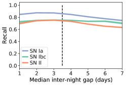
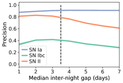
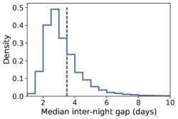
Figure 8: WFD test set recall (left panel) and precision (middle panel) as a function of median inter-night gap per SNe class for events with light curves between $50$ and $175$ days long. In general, the recall and precision are higher for events whose median inter-night gap is $<3.5$ days (left side of the black line). The right panel shows the density of events as a function of median inter-night gap; $\sim 64\%$ of SN Ia, $\sim 63\%$ of SN Ibc, and $\sim 66\%$ of SN II from the test set events have median inter-night gap $<3.5$ days and light curve lengths between $50$ and $175$ days.

5.3 Inter-night Gaps

The cadence of observation, as quantified by the inter-night gap when no observations are taken in any passband, is a critical factor in LSST observing strategy that impacts all transient science goals. To investigate this effect, we compared the performance of SNe with different median inter-night gap. The left panel of Figure 8 shows that cadence has an important impact on SNe classification; events whose median inter-night gap is $<3.5$ days yield higher recall and precision. Such events comprise nearly $70\%$ of the entire test set. These events are better sampled and thus have a higher light curve quality. Moreover, for a fixed SN Ia recall of $80\%$, the core-collapse SN contamination is $6.8\%$ for events whose median inter-night gap is $<3.5$ days, and $8.0\%$ otherwise. These results support previous works such as Lochner et al. (2018, 2021) that call for SN Ia light curves to have frequent observations in order to reduce the uncertainty on the cosmological distance modulus.

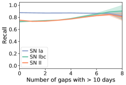
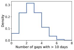
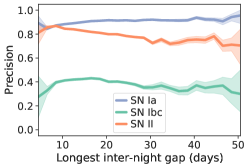
Figure 9: WFD test set recall (left panels) and precision (middle panels) as a function of the number of gaps longer than $10$ days (top row) and the length of the longest inter-night gap (bottom row), per SNe class. We only included events with median inter-night gap $<3.5$ days and light curves between $50$ and $175$ days long. These results show that large gaps do not significantly impact the SNe classification for this subset. The right panel shows the density of events as a function of the number of large gaps (top row) and the length of the longest inter-night gap (bottom row). We note that the results in the tails of the distribution are dominated by small-number effects.

However, the median inter-night gap does not fully capture the impact of gaps in the light curve. A $3.5$-day median inter-night gap does not imply a uniform cadence; it is entirely possible that such light curves contain much larger gaps. To investigate the impact of such ‘gappy’ light curves, we studied the classification performance as a function of the number of large gaps ($>10$ days) in a subsample of events with a median inter-night gap $<3.5$ days.

The upper left panels of Figure 9 show the recall and precision are broadly independent of the number of large gaps in a light curve. We tested this with $>20$-day gaps and found similar results.

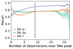
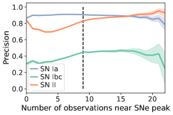
Figure 10: WFD test set recall (left panel) and precision (middle panel) as a function of the number of observation between $10$ days before and $30$ days after the peak per SNe class. We only included events with median inter-night gap $<3.5$ days and light curves between $50$ and $175$ days long. In general, the recall and precision increase with the number of observations near the peak, until they reach an approximately constant value for events with $\geq 9$ observations. The right panel shows the density of events as a function of number of observations near peak. We note that, as with previous plots, the results in the tails of the distribution are dominated by small-number effects.

We expect that the reason for these surprising findings is that the GP fits can still constrain a light curve fit sufficiently well if there are enough points on either side of large gaps. This is demonstrated in Figure 2, which shows an example of a GP fit to an event with four gaps $>10$ days, one of which is $>20$ days. We then compare the classification performance as a function of the length of the longest inter-night gap per light curve, to investigate at which point the performance degrades due to inability of GP fits to constrain a light curve fit. The bottom panels of Figure 9 show that the recall and precision of SNe either slowly decrease or remain constant with the increase of the length of longest inter-night gap. While previous works recommended a regular cadence without inter-night gaps larger than $10$ – $15$ days (Lochner et al., 2018, 2021), we find that requiring a median inter-night gap of $<3.5$ days is sufficient for photometric classification methods using GPs that incorporate cross-band information to model the light curves and generate features.

We also find that 98% of DDF events have a median inter-night gap of $<3.5$ days, and hence the DDF sample performs uniformly well independent of the inter-night gap.

5.4 Observations Near Peak

Obtaining observations near the peak of a SN Ia light curve is generally considered critical to obtain a reliable cosmological distance modulus. To investigate whether SNe classification has a similar requirement, we analyzed the classification performance as a function of the number of observations near the peak (defined as $10$ days before and $30$ days after the peak). We estimated the peak time as the moment that maximizes the GP fit predicted flux. Figure 10 shows that the recall and precision generally increase with the number of observations near the peak, reaching a constant value for events with more than nine observations. This improvement in performance is likely due to better characterization of light curve shape. However, since we cannot predict when a SN will be observed, this result only further demonstrates the importance of frequent observations to increase the likelihood of obtaining observations near the peak. These results agree with Takahashi et al. (2020), who found that SNe light curves without observations near the peak were more often misclassified.

6 Discussion and Conclusions

We have presented a quantitative analysis of the impact of various factors related to the LSST observing strategy on the performance of SNe photometric classification, using the PLAsTiCC simulation. We use the photometric transient classification library snmachine, based on model-independent wavelet features (instead of specialized features constructed using domain knowledge about SNe). In line with previous studies using the PLAsTiCC data, we confirm that augmentation for a number of aspects (the photometric redshift distribution per supernovae class, the distribution of the observing cadence, and the flux uncertainty distribution) is crucial for obtaining a representative training set for machine learning classification.

Our classifier yields similar performance to the top PLAsTiCC submission (Boone, 2019; Hložek et al., 2020) and competitive results in core-collapse SN contamination (see below; Kessler & Scolnic, 2017; Jones et al., 2017), which is essential for measurements of the dark energy equation of state parameter. We obtain a core-collapse SN contamination of $8.3\%$ (for SNe predicted to be SN Ia with $>50\%$ probability) which is comparable to the $\sim 5\%$ contamination obtained in Jones et al. (2018) with Pan-STARRS SNe. This could be further improved by optimizing the classifier for SN Ia classification rather than overall classification performance as was done in PLAsTiCC. Jones et al. (2018) demonstrated that this level of contamination provides competitive cosmological constraints when using a Bayesian methodology to marginalize over the contamination. Hence, we expect our contamination levels to also be acceptable for cosmology when used along with a Bayesian methodology such as Bayesian Estimation Applied to Multiple Species (Kunz et al., 2007; Lochner et al., 2013; Roberts et al., 2017; Jones et al., 2018).

Turning to the question of how observing strategy impacts classification, our results demonstrate the importance of customized training set augmentation for each LSST survey mode (WFD and DDF). We find that the season length is important – in general, better classification performance is obtained for longer light curves. This supports the minimum five-month season length recommendation in Lochner et al. (2018, 2021). Further, we show that good classification performance requires a cadence with a median inter-night gap of $<3.5$ days. Surprisingly, however, we find that large gaps of $>10$ days do not impact the classification performance for events exhibiting such a cadence, due to the ability of the Gaussian process methods we use to interpolate such gaps effectively. Finally, a regular cadence which achieves $>9$ observations near the peak of the light curve provides effective classification performance. In Appendix B we show that these results also hold if we replace our classification predictions with the predictions obtained by Boone (2019), who use a different feature set and an independent classification framework with somewhat different augmentation choices.

These results provide guidance for further refinement of the LSST observing strategy on the question of SNe photometric classification. While the PLAsTiCC simulation used in this analysis has an outdated cadence, we expect our general conclusions to hold for any reasonable variation currently under consideration. Our augmentation and classification pipeline will be used in the future to study the SNe classification performance of more recent observing strategy simulations in detail.

Since the release of PLAsTiCC, new and more realistic observing strategy simulations have been released. These simulations include improvements to the scheduler, more realistic weather, and changes to the cadence in different bands. While new transient simulations using the more recent baseline observing strategy may result in different classification performance, we still expect our broad conclusions to remain unchanged. Future work will include investigating the dependence of classification performance on different observing strategy simulations.

With this paper we publicly release the photometric transient classification library snmachine. The library also contains some example Jupyter notebooks which can be used to reproduce this work. In the future, the snmachine pipeline will be extended to facilitate the classification of other transient classes.

Appendix A Redshifting Implementation for Augmentation

In this appendix we provide further details of the augmentation procedure described in Section 4. In particular, we present the technique for redshifting a light curve, and derive the redshift limits for augmentation shown in Equation (4).

Consider a multi-band SN light curve at redshift $z_{\mathrm{ori}}$, from which we want to create a synthetic multi-band light curve at redshift $z_{\mathrm{aug}}$. For each epoch, the spectrum of the new synthetic SN is

$$f_{\lambda;\,\mathrm{aug}}(\lambda)=\dfrac{1+z_{\mathrm{ori}}}{1+z_{\mathrm{aug}}}\left[\dfrac{d_{\mathrm{L}}\left(z_{\mathrm{ori}}\right)}{d_{\mathrm{L}}\left(z_{\mathrm{aug}}\right)}\right]^{2}f_{\lambda}\left(\dfrac{1+z_{\mathrm{ori}}}{1+z_{\mathrm{aug}}}\lambda\right)\,,\,$$ (A1)

where $\lambda$ is the observed wavelength, $d_{\mathrm{L}}$ is the luminosity distance, and $f_{\lambda}$ is the spectrum of the original event. Note that the spectrum of the synthetic SN depends on the original spectrum evaluated at redshifted wavelengths. The two-dimensional GP fit described in Section 3.2 then models the convolution of the original spectrum with the ugrizy passbands to predict the measured flux. Thus, for each epoch of the synthetic SN, we estimated the flux in the original event at each redshifted passband $\mathrm{b}$ (where $\mathrm{b}=u,g,r,i,z,y$) as

$$F_{\mathrm{ori\,b}}=\mathcal{GP}\left(\dfrac{1+z_{\mathrm{ori}}}{1+z_{\mathrm{aug}}}\lambda_{\mathrm{b}}\right)\,,$$ (A2)

where $\mathcal{GP}$ represents the mean of the GP fit used to model the flux observations of the original SNe, and $\lambda_{\mathrm{b}}$ is the central wavelength of passband $\mathrm{b}$. We calculated these central wavelengths using the LSST throughputs. Similarly, we estimated the flux uncertainty in each passband as the uncertainty of the GP fit.

Finally, we adjusted the fluxes of the synthetic event and their uncertainties to the desired redshift $z_{\mathrm{aug}}$. We assumed a flat $\Lambda$CDM cosmology with $H_{0}=70$ km/s/Mpc and $\Omega_{\mathrm{m}}=0.3$. We estimated the flux of the synthetic event in each passband $\mathrm{b}$ as

$$F_{\mathrm{aug\,b}}=\dfrac{1+z_{\mathrm{ori}}}{1+z_{\mathrm{aug}}}\left[\dfrac{d_{\mathrm{L}}\left(z_{\mathrm{ori}}\right)}{d_{\mathrm{L}}\left(z_{\mathrm{aug}}\right)}\right]^{2}F_{\mathrm{ori\,b}}\,,$$ (A3)

and estimated its uncertainty similarly.

As previously discussed in Section 4.2, the GP fit is more reliable close to observations. To test the GP extrapolation, for every SNe in the training set, we fitted a GP with the observations in the ugriz passbands. Then, we compared the observed flux in the y passband with the flux predictions of the GP fit at the same epochs. Additionally, we repeated this procedure to test the GP extrapolation in the u passband using the observations in the grizy passbands. Figure 11 shows the GP is reliable despite underestimating some flux errors. Since the GP errors increase at wavelengths far from the original observation, we restricted our extrapolation to minimum ($\lambda_{g}-\lambda_{u}$) and maximum ($\lambda_{y}-\lambda_{z}$) wavelength ranges. Thus, when generating a synthetic SN at higher redshifts, we have that $\lambda_{u}-(1+z_{\mathrm{ori}})/(1+z_{\mathrm{aug}})\lambda_{u}\leq\lambda_{g}-\lambda_{u}$. Similarly, for events generated at lower redshifts, we obtain the redshift limits for augmentation presented in Section 4.2:

$$\begin{aligned} z_{\mathrm{min}}&=\max\left\{0,\left(1+z_{\mathrm{ori}}\right)\left(2-\dfrac{\lambda_{\mathrm{z}}}{\lambda_{\mathrm{y}}}\right)^{-1}-1\right\}\\ &\approx\max\left\{0,0.90\,z_{\mathrm{ori}}-0.10\right\}\,,\\ z_{\mathrm{max}}&=\left(1+z_{\mathrm{ori}}\right)\left(2-\dfrac{\lambda_{\mathrm{g}}}{\lambda_{\mathrm{u}}}\right)^{-1}-1\\ &\approx 1.43\,z_{\mathrm{ori}}+0.43\,.\end{aligned}\,.$$ (A4)

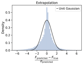
Figure 11: Distribution of the GP errors resulting from extrapolating GP fits to u or y passbands. $F_{\mathrm{true}}$ is the true flux of an observation, and $F_{\mathrm{predicted}}$ and $\sigma_{\mathrm{predicted}}$ are the flux and its uncertainty predicted by a GP fit at the corresponding epoch and passband. An ideal error estimation results in a unit Gaussian (black line).

Appendix B Comparison with other PLASTICC classifiers

Section 5 presented the results of our classifier on the impact of observing strategy on photometric classification. In this appendix, we show that our results are generalizable beyond our classification pipeline, by replacing the our classification predictions with those obtained by Boone (2019). We use the publicly available predictions for SN Ia, SN Ibc, and SN II in the test set; we choose the predictions obtained with a classifier optimized on the log-loss metric, which equally weights all the PLAsTiCC classes ($w_{i}=1$ in Equation 1). The choice of this flat-weighted metric reduces the impact of additional classes upweighted in the original challenge, but unused in the present work. Figures 12 and 13 show that the classifier used in Boone (2019) has the same performance behavior as ours. This further indicates that our conclusions are general and not an artifact of our classification architecture.

Classification predictions from present work

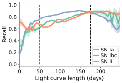
Classification predictions from Boone (2019)

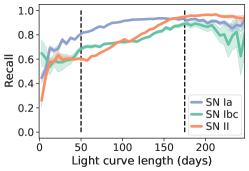
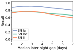
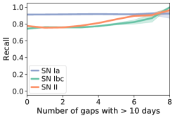
Classification predictions from present work

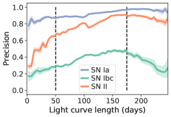
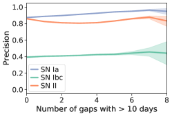
Classification predictions from Boone (2019)

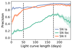
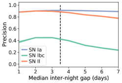
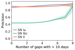
Figure 12: WFD test set recall (top two rows) and precision (bottom two rows) as a function of light curve length (left panels), median inter-night gap (middle panels), and number of gaps larger than $10$ days (right panels), per SNe class. In the first and third rows we reproduce the results of this work previously shown in Figures 7, 8, and 9. In the second and fourth rows we show the classification predictions obtained by Boone (2019).

Classification predictions from present work

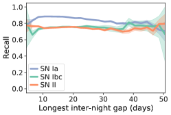
Classification predictions from Boone (2019)

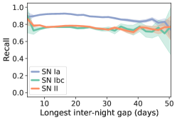
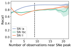
Classification predictions from present work

Classification predictions from Boone (2019)

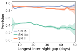
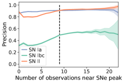
Figure 13: WFD test set recall (top two rows) and precision (bottom two rows) as a function of the length of the longest inter-night gap (left panels) and the number of observations between $10$ days before and $30$ days after the peak length (right panels), per SNe class. In the first and third rows we reproduce the results of this work previously shown in Figures 9 and 10. In the second and fourth rows we show the classification predictions obtained by Boone (2019).

References

- Ambikasaran et al. (2014) Ambikasaran, S., Foreman-Mackey, D., Greengard, L., Hogg, D. W., & O’Neil, M. 2014, arXiv preprint arXiv:1403.6015v2. http://arxiv.org/abs/1403.6015
- Astier et al. (2006) Astier, P., Guy, J., Regnault, N., et al. 2006, Astronomy & Astrophysics, 447, 31, doi: 10.1051/0004-6361:20054185
- Astropy Collaboration et al. (2013) Astropy Collaboration, Robitaille, T. P., Tollerud, E. J., et al. 2013, Astronomy & Astrophysics, 558, A33, doi: 10.1051/0004-6361/201322068
- Astropy Collaboration et al. (2018) Astropy Collaboration, Price-Whelan, A. M., Sipőcz, B. M., et al. 2018, The Astronomical Journal, 156, 123, doi: 10.3847/1538-3881/aabc4f
- Barbier et al. (2016) Barbier, J., Dia, M., Macris, N., et al. 2016, in Advances in Neural Information Processing Systems, ed. D. Lee, M. Sugiyama, U. Luxburg, I. Guyon, & R. Garnett, Vol. 29 (Curran Associates, Inc.). https://proceedings.neurips.cc/paper/2016/file/621bf66ddb7c962aa0d22ac97d69b793-Paper.pdf
- Boone (2019) Boone, K. 2019, The Astronomical Journal, 158, 257, doi: 10.3847/1538-3881/ab5182
- Carrick et al. (2021) Carrick, J. E., Hook, I. M., Swann, E., et al. 2021, Monthly Notices of the Royal Astronomical Society, doi: 10.1093/mnras/stab2343
- Caswell et al. (2020) Caswell, T. A., Droettboom, M., Lee, A., et al. 2020, matplotlib/matplotlib: REL: v3.3.2, Zenodo, doi: 10.5281/ZENODO.4030140
- Charnock & Moss (2017) Charnock, T., & Moss, A. 2017, The Astrophysical Journal, 837, L28, doi: 10.3847/2041-8213/aa603d
- Chen et al. (2013) Chen, N., Qian, Z., & Meng, X. 2013, Mathematical Problems in Engineering, 2013, 1, doi: 10.1155/2013/461983
- Friedman (2001) Friedman, J. H. 2001, The Annals of Statistics, 29, 1189, doi: 10.1214/aos/1013203451
- Gonzalez et al. (2018) Gonzalez, O. A., Clarkson, W., Debattista, V. P., et al. 2018, arXiv preprint arXiv:1812.08670
- Guillochon et al. (2017) Guillochon, J., Parrent, J., Kelley, L. Z., & Margutti, R. 2017, The Astrophysical Journal, 835, 64, doi: 10.3847/1538-4357/835/1/64
- Harris et al. (2020) Harris, C. R., Millman, K. J., van der Walt, S. J., et al. 2020, Nature, 585, 357, doi: 10.1038/s41586-020-2649-2
- Hložek et al. (2020) Hložek, R., Ponder, K. A., Malz, A. I., et al. 2020, arXiv preprint arXiv:2012.12392
- Hotelling (1933) Hotelling, H. 1933, Journal of Educational Psychology, 24, 417, doi: 10.1037/h0071325
- Hunter (2007) Hunter, J. D. 2007, Computing in Science & Engineering, 9, 90, doi: 10.1109/MCSE.2007.55
- Istas (1992) Istas, J. 1992, Annales de l’I.H.P. Probabilités et statistiques, 28, 537. http://www.numdam.org/item/AIHPB_1992__28_4_537_0/
- Ivezić et al. (2018) Ivezić, Ž., Jones, L., & Ribeiro, T. 2018, Call for White Papers on LSST Cadence Optimization
- Ivezić et al. (2019) Ivezić, Ž., Kahn, S. M., Tyson, J. A., et al. 2019, The Astrophysical Journal, 873, 111, doi: 10.3847/1538-4357/ab042c
- Jones et al. (2017) Jones, D. O., Scolnic, D. M., Riess, A. G., et al. 2017, The Astrophysical Journal, 843, 6, doi: 10.3847/1538-4357/aa767b
- Jones et al. (2018) —. 2018, The Astrophysical Journal, 857, 51, doi: 10.3847/1538-4357/aab6b1
- Jones et al. (2020) Jones, R. L., Yoachim, P., Ivezic, Z., Neilsen, E. H., & Ribeiro, T. 2020, Survey Strategy and Cadence Choices for the Vera C. Rubin Observatory Legacy Survey of Space and Time (LSST), Tech. rep., doi: 10.5281/ZENODO.4048838
- Ke et al. (2017) Ke, G., Meng, Q., Finley, T., et al. 2017, in Advances in Neural Information Processing Systems 30, ed. I. Guyon, U. V. Luxburg, S. Bengio, H. Wallach, R. Fergus, S. Vishwanathan, & R. Garnett, Vol. 30 (Curran Associates, Inc.), 3146–3154
- Kessler et al. (2010a) Kessler, R., Conley, A., Jha, S., & Kuhlmann, S. 2010a, arXiv preprint arXiv:1001.5210
- Kessler & Scolnic (2017) Kessler, R., & Scolnic, D. 2017, The Astrophysical Journal, 836, 56, doi: 10.3847/1538-4357/836/1/56
- Kessler et al. (2009) Kessler, R., Becker, A. C., Cinabro, D., et al. 2009, The Astrophysical Journal Supplement Series, 185, 32, doi: 10.1088/0067-0049/185/1/32
- Kessler et al. (2010b) Kessler, R., Bassett, B., Belov, P., et al. 2010b, Publications of the Astronomical Society of the Pacific, 122, 1415, doi: 10.1086/657607
- Kessler et al. (2019) Kessler, R., Narayan, G., Avelino, A., et al. 2019, Publications of the Astronomical Society of the Pacific, 131, 094501, doi: 10.1088/1538-3873/ab26f1
- Kluyver et al. (2016) Kluyver, T., Ragan-Kelley, B., Pérez, F., et al. 2016, in Positioning and Power in Academic Publishing: Players, Agents and Agendas, ed. F. Loizides & B. Scmidt (Netherlands: IOS Press), 87–90. https://eprints.soton.ac.uk/403913/
- Krekel et al. (2004) Krekel, H., Oliveira, B., Pfannschmidt, R., et al. 2004, pytest 6.2.2. https://github.com/pytest-dev/pytest
- Kunz et al. (2007) Kunz, M., Bassett, B. A., & Hlozek, R. 2007, Physical Review D, 75, 103508, doi: 10.1103/PhysRevD.75.103508
- Laine et al. (2018) Laine, S., Martinez-Delgado, D., Trujillo, I., et al. 2018, arXiv preprint arXiv:1812.04897
- Lee et al. (2019a) Lee, G., Gommers, R., Waselewski, F., Wohlfahrt, K., & O’Leary, A. 2019a, Journal of Open Source Software, 4, 1237, doi: 10.21105/joss.01237
- Lee et al. (2019b) Lee, G. R., Gommers, R., Wohlfahrt, K., et al. 2019b, PyWavelets/pywt: PyWavelets 1.1.1, Zenodo, doi: 10.5281/ZENODO.3510098
- Lochner et al. (2013) Lochner, M., Bassett, B. A., Varughese, M., et al. 2013, Journal of Cosmology and Astroparticle Physics, 2013, 039, doi: 10.1088/1475-7516/2013/01/039
- Lochner et al. (2016) Lochner, M., McEwen, J. D., Peiris, H. V., Lahav, O., & Winter, M. K. 2016, The Astrophysical Journal Supplement Series, 225, 31
- Lochner et al. (2018) Lochner, M., Scolnic, D. M., Awan, H., et al. 2018, arXiv preprint arXiv:1812.00515
- Lochner et al. (2021) Lochner, M., Scolnic, D., Almoubayyed, H., et al. 2021, arXiv preprint arXiv:2104.05676. https://arxiv.org/abs/2104.05676
- LSST Science Collaboration et al. (2009) LSST Science Collaboration, Abell, P. A., Allison, J., et al. 2009, arXiv preprint arXiv:0912.0201
- LSST Science Collaboration et al. (2017) LSST Science Collaboration, Marshall, P., Anguita, T., et al. 2017, arXiv preprint arXiv:1708.04058, doi: 10.5281/zenodo.842713
- MacKay (2003) MacKay, D. J. C. 2003, Information Theory, Inference and Learning Algorithms (Cambridge University Pr.)
- Malz et al. (2019) Malz, A. I., Hložek, R., Allam, T., et al. 2019, The Astronomical Journal, 158, 171, doi: 10.3847/1538-3881/ab3a2f
- Mockus et al. (1978) Mockus, J., Tiesis, V., & Zilinskas, A. 1978, Towards Global Optimization, 2, 2
- Muthukrishna et al. (2019) Muthukrishna, D., Narayan, G., Mandel, K. S., Biswas, R., & Hložek, R. 2019, Publications of the Astronomical Society of the Pacific, 131, 118002, doi: 10.1088/1538-3873/ab1609
- Narayan et al. (2018) Narayan, G., Zaidi, T., Soraisam, M. D., et al. 2018, The Astrophysical Journal Supplement Series, 236, 9, doi: 10.3847/1538-4365/aab781
- pandas development team (2020) pandas development team, T. 2020, pandas-dev/pandas: Pandas, latest, Zenodo, doi: 10.5281/zenodo.3509134
- Pasquet et al. (2019) Pasquet, J., Pasquet, J., Chaumont, M., & Fouchez, D. 2019, Astronomy & Astrophysics, 627, A21, doi: 10.1051/0004-6361/201834473
- Pearson (1901) Pearson, K. 1901, The London, Edinburgh, and Dublin Philosophical Magazine and Journal of Science, 2, 559, doi: 10.1080/14786440109462720
- Pedregosa et al. (2011) Pedregosa, F., Varoquaux, G., Gramfort, A., et al. 2011, Journal of Machine Learning Research, 12, 2825
- PLAsTiCC Modelers (2019) PLAsTiCC Modelers. 2019, Libraries & Recommended Citations for using PLAsTiCC Models, Zenodo, doi: 10.5281/ZENODO.2612896
- PLAsTiCC Team & PLAsTiCC Modelers (2019) PLAsTiCC Team, & PLAsTiCC Modelers. 2019, Unblinded Data for PLAsTiCC Classification Challenge, Zenodo, doi: 10.5281/ZENODO.2535746
- Pope (2019) Pope, C. A. 2019, PhD thesis, University of Leeds. https://etheses.whiterose.ac.uk/25066/
- Rasmussen & Williams (2005) Rasmussen, C. E., & Williams, C. K. I. 2005, Gaussian Processes for Machine Learning (MIT Press Ltd)
- Revsbech et al. (2017) Revsbech, E. A., Trotta, R., & van Dyk, D. A. 2017, Monthly Notices of the Royal Astronomical Society, 473, 3969, doi: 10.1093/mnras/stx2570
- Riess et al. (1998) Riess, A. G., Filippenko, A. V., Challis, P., et al. 1998, The Astronomical Journal, 116, 1009, doi: 10.1086/300499
- Roberts et al. (2017) Roberts, E., Lochner, M., Fonseca, J., et al. 2017, Journal of Cosmology and Astroparticle Physics, 2017, 036, doi: 10.1088/1475-7516/2017/10/036
- Scolnic et al. (2018) Scolnic, D. M., Lochner, M., Gris, P., et al. 2018, arXiv preprint arXiv:1812.00516
- Snoek et al. (2012) Snoek, J., Larochelle, H., & Adams, R. P. 2012, arXiv preprint arXiv:1206.2944
- Sooknunan et al. (2021) Sooknunan, K., Lochner, M., Bassett, B. A., et al. 2021, Monthly Notices of the Royal Astronomical Society, 502, 206, doi: 10.1093/mnras/staa3873
- Swann et al. (2019) Swann, E., Sullivan, M., Carrick, J., et al. 2019, The Messenger vol. 175, pp. 58-61, March 2019., doi: 10.18727/0722-6691/5129
- Takahashi et al. (2020) Takahashi, I., Suzuki, N., Yasuda, N., et al. 2020, Publications of the Astronomical Society of Japan, 72, doi: 10.1093/pasj/psaa082
- The Dark Energy Survey Collaboration & Flaugher (2005) The Dark Energy Survey Collaboration, & Flaugher, B. 2005, International Journal of Modern Physics A, 20, 3121, doi: 10.1142/s0217751x05025917
- The PLAsTiCC team et al. (2018) The PLAsTiCC team, Allam Jr, T., Bahmanyar, A., et al. 2018, arXiv preprint arXiv:1810.00001
- Van Rossum (2020) Van Rossum, G. 2020, The Python Library Reference, release 3.8.2 (Python Software Foundation)
- Varughese et al. (2015) Varughese, M. M., von Sachs, R., Stephanou, M., & Bassett, B. A. 2015, Monthly Notices of the Royal Astronomical Society, 453, 2849, doi: 10.1093/mnras/stv1816
- Villar et al. (2020) Villar, V. A., Hosseinzadeh, G., Berger, E., et al. 2020, The Astrophysical Journal, 905, 94, doi: 10.3847/1538-4357/abc6fd
- Virtanen et al. (2020) Virtanen, P., Gommers, R., Oliphant, T. E., et al. 2020, Nature Methods, 17, 261, doi: 10.1038/s41592-019-0686-2
- Waskom et al. (2020) Waskom, M., Botvinnik, O., Gelbart, M., et al. 2020, mwaskom/seaborn: v0.11.0 (Sepetmber 2020), Zenodo, doi: 10.5281/ZENODO.4019146
- Wes McKinney (2010) Wes McKinney. 2010, in Proceedings of the 9th Python in Science Conference, ed. Stéfan van der Walt & Jarrod Millman, 56 – 61, doi: 10.25080/Majora-92bf1922-00a
- Zhang et al. (2017) Zhang, H., Si, S., & Hsieh, C.-J. 2017, arXiv preprint arXiv:1706.08359