Newton-LESS: Sparsification without Trade-offs
for the Sketched Newton Update

Michał Dereziński Department of Statistics, University of California, Berkeley (mderezin@berkeley.edu)    Jonathan Lacotte Department of Electrical Engineering, Stanford University (lacotte@stanford.edu)    Mert Pilanci Department of Electrical Engineering, Stanford University (pilanci@stanford.edu)    Michael W. Mahoney ICSI and Department of Statistics, University of California, Berkeley (mmahoney@stat.berkeley.edu)
Abstract

In second-order optimization, a potential bottleneck can be computing the Hessian matrix of the optimized function at every iteration. Randomized sketching has emerged as a powerful technique for constructing estimates of the Hessian which can be used to perform approximate Newton steps. This involves multiplication by a random sketching matrix, which introduces a trade-off between the computational cost of sketching and the convergence rate of the optimization algorithm. A theoretically desirable but practically much too expensive choice is to use a dense Gaussian sketching matrix, which produces unbiased estimates of the exact Newton step and which offers strong problem-independent convergence guarantees. We show that the Gaussian sketching matrix can be drastically sparsified, significantly reducing the computational cost of sketching, without substantially affecting its convergence properties. This approach, called Newton-LESS, is based on a recently introduced sketching technique: LEverage Score Sparsified (LESS) embeddings. We prove that Newton-LESS enjoys nearly the same problem-independent local convergence rate as Gaussian embeddings, not just up to constant factors but even down to lower order terms, for a large class of optimization tasks. In particular, this leads to a new state-of-the-art convergence result for an iterative least squares solver. Finally, we extend LESS embeddings to include uniformly sparsified random sign matrices which can be implemented efficiently and which perform well in numerical experiments.

1 Introduction

Consider the task of minimizing a twice-differentiable convex function f:d:𝑓superscript𝑑f:\mathbb{R}^{d}\rightarrow\mathbb{R}:

find𝐱=argmin𝐱df(𝐱).findsuperscript𝐱subscriptargmin𝐱superscript𝑑𝑓𝐱\displaystyle\text{find}\quad\mathbf{x}^{*}=\operatorname*{\mathop{\mathrm{argmin}}}_{\mathbf{x}\in\mathbb{R}^{d}}f(\mathbf{x}).

One of the most classical iterative algorithms for solving this task is the Newton’s method, which takes steps of the form 𝐱t+1=𝐱tμt2f(𝐱t)1f(𝐱t)subscript𝐱𝑡1subscript𝐱𝑡subscript𝜇𝑡superscript2𝑓superscriptsubscript𝐱𝑡1𝑓subscript𝐱𝑡\mathbf{x}_{t+1}=\mathbf{x}_{t}-\mu_{t}\nabla^{2}f(\mathbf{x}_{t})^{-1}\nabla f(\mathbf{x}_{t}), and which leverages second-order information in the d×d𝑑𝑑d\times d Hessian matrix 2f(𝐱t)superscript2𝑓subscript𝐱𝑡\nabla^{2}f(\mathbf{x}_{t}) to achieve rapid convergence, especially locally as it approaches the optimum 𝐱superscript𝐱\mathbf{x}^{*}. However, in many settings, the cost of forming the exact Hessian is prohibitively expensive, particularly when the function f𝑓f is given as a sum of ndmuch-greater-than𝑛𝑑n\gg d components, i.e., f(𝐱)=i=1nfi(𝐱)𝑓𝐱superscriptsubscript𝑖1𝑛subscript𝑓𝑖𝐱f(\mathbf{x})=\sum_{i=1}^{n}f_{i}(\mathbf{x}). This commonly arises in machine learning when f𝑓f represents the training loss over a dataset of n𝑛n elements, as well as in solving semi-definite programs, portfolio optimization, and other tasks. In these contexts, we can represent the Hessian via a decomposition 2f(𝐱)=𝐀f(𝐱)𝐀f(𝐱)superscript2𝑓𝐱subscript𝐀𝑓superscript𝐱topsubscript𝐀𝑓𝐱\nabla^{2}f(\mathbf{x})={\mathbf{A}_{f}(\mathbf{x})}^{{\scriptscriptstyle{\top}}}{\mathbf{A}_{f}(\mathbf{x})}, where 𝐀f(𝐱)subscript𝐀𝑓𝐱{\mathbf{A}_{f}(\mathbf{x})} is a tall n×d𝑛𝑑n\times d matrix, which can be easily formed, and the main bottleneck is the matrix multiplication which takes O(nd2)𝑂𝑛superscript𝑑2O(nd^{2}) arithmetic operations. To avoid this bottleneck, many randomized second-order methods have been proposed which use a Hessian estimate in place of the exact Hessian (e.g., [BCNN11, EM15, ABH17, RKM19]). This naturally leads to a trade-off between the per-iteration cost of the method and the number of iterations needed to reach convergence. We develop Newton-LESS, a randomized second-order method which eliminates the computational bottleneck while minimizing the convergence trade-offs.

An important family of approximate second-order methods is known as the Newton Sketch [PW17]:

𝐱~t+1=𝐱~tμt(𝐀f(𝐱~t)𝐒t𝐒t𝐀f(𝐱~t))1f(𝐱~t),subscript~𝐱𝑡1subscript~𝐱𝑡subscript𝜇𝑡superscriptsubscript𝐀𝑓superscriptsubscript~𝐱𝑡topsuperscriptsubscript𝐒𝑡topsubscript𝐒𝑡subscript𝐀𝑓subscript~𝐱𝑡1𝑓subscript~𝐱𝑡\displaystyle\widetilde{\mathbf{x}}_{t+1}=\widetilde{\mathbf{x}}_{t}-\mu_{t}\big{(}{\mathbf{A}_{f}(\widetilde{\mathbf{x}}_{t})}^{\scriptscriptstyle{\top}}\mathbf{S}_{t}^{\scriptscriptstyle{\top}}\mathbf{S}_{t}{\mathbf{A}_{f}(\widetilde{\mathbf{x}}_{t})}\big{)}^{-1}\nabla f(\widetilde{\mathbf{x}}_{t}), (1)

where μtsubscript𝜇𝑡\mu_{t} is the step size, and 𝐒tsubscript𝐒𝑡\mathbf{S}_{t} is a random m×n𝑚𝑛m\times n sketching matrix, with mnmuch-less-than𝑚𝑛m\ll n, that is used to reduce 𝐀f(𝐱~t)subscript𝐀𝑓subscript~𝐱𝑡{\mathbf{A}_{f}(\widetilde{\mathbf{x}}_{t})} to a small m×d𝑚𝑑m\times d sketch 𝐒t𝐀f(𝐱~t)subscript𝐒𝑡subscript𝐀𝑓subscript~𝐱𝑡\mathbf{S}_{t}{\mathbf{A}_{f}(\widetilde{\mathbf{x}}_{t})}. This brings the complexity of forming the Hessian down to O(md2)𝑂𝑚superscript𝑑2O(md^{2}) time plus the cost of forming the sketch.

Naturally, sketching methods vary in their computational cost and they can affect the convergence rate, so the right choice of 𝐒tsubscript𝐒𝑡\mathbf{S}_{t} depends on the computation-convergence trade-off. On one end of this spectrum are the so-called Sub-Sampled Newton methods [RKM19, XRKM17, YXRKM18], where 𝐒tsubscript𝐒𝑡\mathbf{S}_{t} simply selects a random sample of m𝑚m rows of 𝐀f(𝐱)subscript𝐀𝑓𝐱{\mathbf{A}_{f}(\mathbf{x})} (e.g., a sample of data points in a training set) to form the sketch. Here the sketching cost is negligible, since 𝐒tsubscript𝐒𝑡\mathbf{S}_{t} is extremely sparse, but the convergence rate can be highly variable and problem-dependent. On the other end, we have what we will refer to as the Gaussian Newton Sketch, where 𝐒tsubscript𝐒𝑡\mathbf{S}_{t} is a dense matrix with i.i.d. scaled Gaussian entries (a.k.a. a Gaussian embedding). While the O(mnd)𝑂𝑚𝑛𝑑O(mnd) cost of performing this sketch limits its practical appeal, Gaussian Newton Sketch has a number of unique and desirable properties [LP19]: it enjoys strong problem-independent convergence rates; it produces unbiased estimates of the exact Newton update (useful in distributed settings); and it admits analytic expressions for the optimal step size.

A natural way to interpolate between these two extremes is to vary the sparsity s𝑠s of the sketching matrix 𝐒tsubscript𝐒𝑡\mathbf{S}_{t}, from s=1𝑠1s=1 non-zero element per row (Sub-Sampling) to s=n𝑠𝑛s=n non-zero elements (Gaussian embedding), with the sketching complexity O(mds)𝑂𝑚𝑑𝑠O(mds).111For a more detailed discussion of other sketching techniques that may not fit this taxonomy, such as the Subsampled Randomized Hadamard Transform and the CountSketch, see Section 1.2. Motivated by this, we ask:

Can we sparsify the Gaussian embedding, making its sparsity closer to that of Sub-Sampling, without suffering any convergence trade-offs?
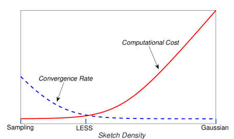
111 non-zero per row of 𝐒𝐒\mathbf{S}Samplingd𝑑d non-zeros per row of 𝐒𝐒\mathbf{S}LESSn𝑛n non-zeros per row of 𝐒𝐒\mathbf{S}Gaussian
Refer to caption
Figure 1: The effect of the density of m×n𝑚𝑛m\times n sketching matrix 𝐒𝐒\mathbf{S} applied to an n×d𝑛𝑑n\times d matrix 𝐀𝐀\mathbf{A} (with d,mnmuch-less-than𝑑𝑚𝑛d,m\ll n) on the convergence rate of Newton Sketch and the computational cost of constructing the Hessian estimate. LESS embeddings “interpolate” between Sub-Sampled Newton methods and Gaussian Newton Sketches, achieving a “sweet spot” in the computation-per-iteration versus number-of-iterations tradeoff.

In this paper, we provide an affirmative answer to this question. We show that it is possible to drastically sparsify the Gaussian embedding so that two key statistics of the sketches, namely first and second inverse moments of the sketched Hessian, are nearly preserved in a very strong sense. Namely, the two inverse moments of the sparse sketches can be upper and lower bounded by the corresponding quantities for the dense Gaussian embeddings, where the upper/lower bounds are matching not just up to constant factors, but down to lower order terms (see Theorem 6). We use this to show that the Gaussian Newton Sketch can be sparsified to the point where the cost of sketching is proportional to the cost of other operations, while nearly preserving the convergence rate (again, down to lower order terms; see Theorem 1). This is illustrated conceptually in Figure 1, showing how the sparsity of the sketch affects the per-iteration convergence rate as well as the computational cost of the Newton Sketch. We observe that while the convergence rate improves as we increase the density, it eventually flattens out. On the other hand, the computational cost stays largely flat until some point when it starts increasing at a linear rate. As a result, there is a sparsity regime where we achieve the best of both worlds: the convergence rate and the computational cost are both nearly at their optimal values, thereby avoiding any trade-off.

To establish our results, we build upon a recently introduced sketching technique called LEverage Score Sparsified (LESS) embeddings [DLDM21]. LESS embeddings use leverage score techniques [DMIMW12a] to provide a carefully-constructed (random) sparsification pattern. This is used to produce a sub-Gaussian embedding with d𝑑d non-zeros per row of 𝐒tsubscript𝐒𝑡\mathbf{S}_{t} (as opposed to n𝑛n for a dense matrix), so that the cost of forming the sketch 𝐒t𝐀f(𝐱~t)subscript𝐒𝑡subscript𝐀𝑓subscript~𝐱𝑡\mathbf{S}_{t}{\mathbf{A}_{f}(\widetilde{\mathbf{x}}_{t})} matches the cost of constructing the Hessian estimate, i.e., O(md2)𝑂𝑚superscript𝑑2O(md^{2}) (see Section 2). [DLDM21] analyzed the first inverse moment of the sketch to show that LESS embeddings retain certain unbiasedness properties of Gaussian embeddings. In our setting, this captures the bias of the Newton Sketch, but it does not capture the variance, which is needed to control the convergence rate.

Contributions.

In this paper, we analyze both the bias and the variance of Newton Sketch with LESS embeddings (Newton-LESS; see Definition 2 and Lemma 7), resulting in a comprehensive convergence analysis. The following are our key contributions:

  1. 1.

    Characterization of the second inverse moment of the sketched Hessian for a class of sketches including sub-Gaussian matrices and LESS embeddings;

  2. 2.

    Precise problem-independent local convergence rates for Newton-LESS, matching the Gaussian Newton Sketch down to lower order terms;

  3. 3.

    Extension of Newton-LESS to regularized minimization tasks, with improved dimension-independent guarantees for the sketch sparsity and convergence rate;

  4. 4.

    Notable corollary: Best known global convergence rate for an iterative least squares solver, which translates to state-of-the-art numerical performance.

1.1 Main results

As our main contribution, we show that, under standard assumptions on the function f(𝐱)𝑓𝐱f(\mathbf{x}), Newton-LESS achieves the same problem-independent local convergence rate as the Gaussian Newton Sketch, despite drastically smaller per-iteration cost.

Theorem 1.

Assume that f(𝐱)𝑓𝐱f(\mathbf{x}) is (a) self-concordant, or (b) has a Lipschitz continuous Hessian. Also, let 𝐇=2f(𝐱)𝐇superscript2𝑓superscript𝐱\mathbf{H}=\nabla^{2}f(\mathbf{x}^{*}) be positive definite. There is a neighborhood U𝑈U containing 𝐱superscript𝐱\mathbf{x}^{*} such that if 𝐱~0Usubscript~𝐱0𝑈\widetilde{\mathbf{x}}_{0}\in U, then Newton-LESS with sketch size mCdlog(dT/δ)𝑚𝐶𝑑𝑑𝑇𝛿m\geq Cd\log(dT/\delta) and step size μt=1dmsubscript𝜇𝑡1𝑑𝑚\mu_{t}=1-\frac{d}{m} satisfies:

(𝔼δ𝐱~T𝐱𝐇2𝐱~0𝐱𝐇2)1/Tϵdmforϵ=O(1d),formulae-sequencesubscriptitalic-ϵsuperscriptsubscript𝔼𝛿superscriptsubscriptnormsubscript~𝐱𝑇superscript𝐱𝐇2superscriptsubscriptnormsubscript~𝐱0superscript𝐱𝐇21𝑇𝑑𝑚foritalic-ϵ𝑂1𝑑\displaystyle\bigg{(}\mathbb{E}_{\delta}\,\frac{\|\widetilde{\mathbf{x}}_{T}-\mathbf{x}^{*}\|_{\mathbf{H}}^{2}}{\|\widetilde{\mathbf{x}}_{0}-\mathbf{x}^{*}\|_{\mathbf{H}}^{2}}\bigg{)}^{1/T}\approx_{\epsilon}\ \frac{d}{m}\qquad\text{for}\quad\epsilon=O\Big{(}\frac{1}{\sqrt{d}}\Big{)},

where 𝔼δXsubscript𝔼𝛿𝑋\mathbb{E}_{\delta}\,X is expectation conditioned on an event that holds with a 1δ1𝛿1-\delta probability, 𝐯𝐌=𝐯𝐌𝐯subscriptnorm𝐯𝐌superscript𝐯top𝐌𝐯\|\mathbf{v}\|_{\mathbf{M}}=\sqrt{\mathbf{v}^{\scriptscriptstyle{\top}}\mathbf{M}\mathbf{v}}, and aϵbsubscriptitalic-ϵ𝑎𝑏a\approx_{\epsilon}b means that |ab|ϵb𝑎𝑏italic-ϵ𝑏|a-b|\leq\epsilon b.

Remark 2.

The same guarantee holds for the Gaussian Newton Sketch, but it is not known for any fast sketching method other than Newton-LESS (see Section 1.2). The alternative assumptions of self-concordance and Lipschitz continuous Hessian are standard in the local convergence analysis of the classical Newton’s method, and they only affect the size of the neighborhood U𝑈U (see Section 4). Global convergence of Newton-LESS follows from existing analysis of the Newton Sketch [PW17].

The notion of expectation 𝔼δsubscript𝔼𝛿\mathbb{E}_{\delta} allows us to accurately capture the average behavior of a randomized algorithm over a moderate (i.e., polynomial in d𝑑d) number of trials even when the true expectation is not well behaved. Here, this guards against the (very unlikely, but non-zero) possibility that the Hessian estimate produced by a sparse sketch will be ill-conditioned.

To illustrate this result in a special case (of obvious independent interest), we provide a simple corollary for the least squares regression task, i.e., f(𝐱)=12𝐀𝐱𝐛2𝑓𝐱12superscriptnorm𝐀𝐱𝐛2f(\mathbf{x})=\frac{1}{2}\|\mathbf{A}\mathbf{x}-\mathbf{b}\|^{2}. Importantly, here the convergence rate of (dm)Tsuperscript𝑑𝑚𝑇(\frac{d}{m})^{T} holds globally. Also, for this task we have 12𝐱𝐱𝐇2=f(𝐱)f(𝐱)12superscriptsubscriptnorm𝐱superscript𝐱𝐇2𝑓𝐱𝑓superscript𝐱\frac{1}{2}\|\mathbf{x}-\mathbf{x}^{*}\|_{\mathbf{H}}^{2}=f(\mathbf{x})-f(\mathbf{x}^{*}), so the convergence can be stated in terms of the excess function value. To our knowledge, this is the best known convergence guarantee for a fast iterative least squares solver.

Corollary 3.

Let f(𝐱)=12𝐀𝐱𝐛2𝑓𝐱12superscriptnorm𝐀𝐱𝐛2f(\mathbf{x})=\frac{1}{2}\|\mathbf{A}\mathbf{x}-\mathbf{b}\|^{2} for 𝐀n×d𝐀superscript𝑛𝑑\mathbf{A}\in\mathbb{R}^{n\times d} and 𝐛n𝐛superscript𝑛\mathbf{b}\in\mathbb{R}^{n}. Then, given any 𝐱~0dsubscript~𝐱0superscript𝑑\widetilde{\mathbf{x}}_{0}\in\mathbb{R}^{d}, Newton-LESS with sketch size mCdlog(dT/δ)𝑚𝐶𝑑𝑑𝑇𝛿m\geq Cd\log(dT/\delta) and step size μt=1dmsubscript𝜇𝑡1𝑑𝑚\mu_{t}=1-\frac{d}{m} satisfies:

(𝔼δf(𝐱~T)f(𝐱)f(𝐱~0)f(𝐱))1/Tϵdmforϵ=O(1d).formulae-sequencesubscriptitalic-ϵsuperscriptsubscript𝔼𝛿𝑓subscript~𝐱𝑇𝑓superscript𝐱𝑓subscript~𝐱0𝑓superscript𝐱1𝑇𝑑𝑚foritalic-ϵ𝑂1𝑑\displaystyle\bigg{(}\mathbb{E}_{\delta}\,\frac{f(\widetilde{\mathbf{x}}_{T})-f(\mathbf{x}^{*})}{f(\widetilde{\mathbf{x}}_{0})-f(\mathbf{x}^{*})}\bigg{)}^{1/T}\approx_{\epsilon}\ \frac{d}{m}\qquad\text{for}\quad\epsilon=O\Big{(}\frac{1}{\sqrt{d}}\Big{)}.

Prior to this work, a convergence rate of (dm)Tsuperscript𝑑𝑚𝑇(\frac{d}{m})^{T} was known only for dense Gaussian embeddings, and only for the least squares task [LP19]. On the other hand, our results apply as generally as the standard local convergence analysis of the Newton’s method, and they include a broad class of sketches. In Section 3, we provide general structural conditions on a randomized sketching matrix that are needed to enable our analysis. These conditions are satisfied by a wide range of sketching methods, including all sub-Gaussian embeddings (e.g., using random sign entries instead of Gaussians), the original LESS embeddings, and other choices of sparse random matrices (see Lemma 7). Moreover, we develop an improved local convergence analysis of the Newton Sketch, which allows us to recover the precise convergence rate and derive the optimal step size. In Appendix D, we also discuss a distributed variant of Newton-LESS, which takes advantage of the near-unbiasedness properties of LESS embeddings, extending the results of [DLDM21].

The performance of Newton-LESS can be further improved for regularized minimization tasks. Namely, suppose that function f𝑓f can be decomposed as follows: f(𝐱)=f0(𝐱)+g(𝐱)𝑓𝐱subscript𝑓0𝐱𝑔𝐱f(\mathbf{x})=f_{0}(\mathbf{x})+g(\mathbf{x}), where g(𝐱)𝑔𝐱g(\mathbf{x}) has a Hessian that is easy to evaluate (e.g., l2subscript𝑙2l_{2}-regularization, g(𝐱)=λ2𝐱2𝑔𝐱𝜆2superscriptnorm𝐱2g(\mathbf{x})=\frac{\lambda}{2}\|\mathbf{x}\|^{2}). In this case, a modified variant of the Newton Sketch has been considered, where only the f0subscript𝑓0f_{0} component is sketched:

𝐱~t+1=𝐱~tμt(𝐀f0(𝐱~t)𝐒t𝐒t𝐀f0(𝐱~t)+2g(𝐱~t))1f(𝐱~t),subscript~𝐱𝑡1subscript~𝐱𝑡subscript𝜇𝑡superscriptsubscript𝐀subscript𝑓0superscriptsubscript~𝐱𝑡topsuperscriptsubscript𝐒𝑡topsubscript𝐒𝑡subscript𝐀subscript𝑓0subscript~𝐱𝑡superscript2𝑔subscript~𝐱𝑡1𝑓subscript~𝐱𝑡\displaystyle\widetilde{\mathbf{x}}_{t+1}=\widetilde{\mathbf{x}}_{t}-\mu_{t}\big{(}{\mathbf{A}_{f_{0}}(\widetilde{\mathbf{x}}_{t})}^{\scriptscriptstyle{\top}}\mathbf{S}_{t}^{\scriptscriptstyle{\top}}\mathbf{S}_{t}{\mathbf{A}_{f_{0}}(\widetilde{\mathbf{x}}_{t})}+\nabla^{2}g(\widetilde{\mathbf{x}}_{t})\big{)}^{-1}\nabla f(\widetilde{\mathbf{x}}_{t}), (2)

where, again, we let 𝐀f0(𝐱)subscript𝐀subscript𝑓0𝐱{\mathbf{A}_{f_{0}}(\mathbf{x})} be an n×d𝑛𝑑n\times d matrix that encodes the second-order information in f0subscript𝑓0f_{0} at 𝐱𝐱\mathbf{x}. For example, in the case of regularized least squares, f(𝐱)=12𝐀𝐱𝐛2+λ2𝐱2𝑓𝐱12superscriptnorm𝐀𝐱𝐛2𝜆2superscriptnorm𝐱2f(\mathbf{x})=\frac{1}{2}\|\mathbf{A}\mathbf{x}-\mathbf{b}\|^{2}+\frac{\lambda}{2}\|\mathbf{x}\|^{2}, we have 𝐀f0(𝐱)=𝐀subscript𝐀subscript𝑓0𝐱𝐀{\mathbf{A}_{f_{0}}(\mathbf{x})}=\mathbf{A} and 2g(𝐱)=λ𝐈superscript2𝑔𝐱𝜆𝐈\nabla^{2}g(\mathbf{x})=\lambda\mathbf{I} for all 𝐱𝐱\mathbf{x}. We show that the convergence rate of both Newton-LESS and the Gaussian Newton Sketch can be improved in the presence of regularization, by replacing the dimension d𝑑d with an effective dimension deffsubscript𝑑eff{d_{\textnormal{eff}}}. This can be significantly smaller than d𝑑d when the Hessian of f0subscript𝑓0f_{0} at the optimum exhibits rapid spectral decay or is approximately low-rank:

deff=tr(2f0(𝐱)2f(𝐱)1)d.subscript𝑑efftrsuperscript2subscript𝑓0superscript𝐱superscript2𝑓superscriptsuperscript𝐱1𝑑\displaystyle{d_{\textnormal{eff}}}=\mathrm{tr}\big{(}\nabla^{2}f_{0}(\mathbf{x}^{*})\,\nabla^{2}f(\mathbf{x}^{*})^{-1}\big{)}\leq d.
Theorem 4.

Assume that f0subscript𝑓0f_{0} and f𝑓f are (a) self-concordant, or (b) have a Lipschitz continuous Hessian. Also, let 2f0(𝐱)superscript2subscript𝑓0superscript𝐱\nabla^{2}f_{0}(\mathbf{x}^{*}) be positive definite and let 2g(𝐱)superscript2𝑔superscript𝐱\nabla^{2}g(\mathbf{x}^{*}) be positive semidefinite, with 𝐇=2f(𝐱)𝐇superscript2𝑓superscript𝐱\mathbf{H}=\nabla^{2}f(\mathbf{x}^{*}). There is a neighborhood U𝑈U containing 𝐱superscript𝐱\mathbf{x}^{*} such that if 𝐱~0Usubscript~𝐱0𝑈\widetilde{\mathbf{x}}_{0}\in U, then Regularized Newton-LESS (2), with sketch size mCdefflog(deffT/δ)𝑚𝐶subscript𝑑effsubscript𝑑eff𝑇𝛿m\geq C{d_{\textnormal{eff}}}\log({d_{\textnormal{eff}}}T/\delta) and step size μt=1deffmsubscript𝜇𝑡1subscript𝑑eff𝑚\mu_{t}=1-\frac{{d_{\textnormal{eff}}}}{m}, satisfies:

(𝔼δ𝐱~T𝐱𝐇2𝐱~0𝐱𝐇2)1/Tdeffm(1+ϵ)forϵ=O(1deff).formulae-sequencesuperscriptsubscript𝔼𝛿superscriptsubscriptnormsubscript~𝐱𝑇superscript𝐱𝐇2superscriptsubscriptnormsubscript~𝐱0superscript𝐱𝐇21𝑇subscript𝑑eff𝑚1italic-ϵforitalic-ϵ𝑂1subscript𝑑eff\displaystyle\bigg{(}\mathbb{E}_{\delta}\,\frac{\|\widetilde{\mathbf{x}}_{T}-\mathbf{x}^{*}\|_{\mathbf{H}}^{2}}{\|\widetilde{\mathbf{x}}_{0}-\mathbf{x}^{*}\|_{\mathbf{H}}^{2}}\bigg{)}^{1/T}\leq\ \frac{{d_{\textnormal{eff}}}}{m}\cdot(1+\epsilon)\qquad\text{for}\quad\epsilon=O\Big{(}\frac{1}{\sqrt{d_{\textnormal{eff}}}}\Big{)}.
Remark 5.

The same guarantee holds for the Gaussian Newton Sketch. Unlike in Theorem 1, here we can only obtain an upper-bound on the local convergence rate, because the exact rate may depend on the starting point 𝐱~0subscript~𝐱0\widetilde{\mathbf{x}}_{0} (see Section 4). For regularized least squares, f(𝐱)=12𝐀𝐱𝐛2+λ2𝐱2𝑓𝐱12superscriptnorm𝐀𝐱𝐛2𝜆2superscriptnorm𝐱2f(\mathbf{x})=\frac{1}{2}\|\mathbf{A}\mathbf{x}-\mathbf{b}\|^{2}+\frac{\lambda}{2}\|\mathbf{x}\|^{2}, the above convergence guarantee holds globally, i.e., U=d𝑈superscript𝑑U=\mathbb{R}^{d}. Note that deffsubscript𝑑eff{d_{\textnormal{eff}}} can be efficiently estimated using sketching-based trace estimators [ACW16, CEM+15].

Finally, our numerical results show that Newton-LESS can be implemented very efficiently on modern hardware platforms, improving on the optimization cost over not only dense Gaussian embeddings, but also state-of-the-art sketching methods such as the Subsampled Randomized Hadamard Transform, as well as other first-order and second-order methods. Moreover, we demonstrate that our theoretical predictions for the optimal sparsity level and convergence rate are extremely accurate in practice.

1.2 Related work

LEverage Score Sparsified (LESS) embeddings were proposed by [DLDM21] as a way of addressing the phenomenon of inversion bias, which arises in distributed second-order methods [WRKXM18, DM19, DBPM20, GGD+21]. Their results only establish the near-unbiasedness of Newton-LESS iterates (i.e., that 𝔼[𝐱~t+1]𝐱t+1𝔼delimited-[]subscript~𝐱𝑡1subscript𝐱𝑡1\mathbb{E}[\widetilde{\mathbf{x}}_{t+1}]\approx\mathbf{x}_{t+1}), but they did not provide any improved guarantees on the convergence rate. Also, their notion of LESS embeddings is much narrower than ours, and so it does not capture Regularized Newton-LESS or uniformly sparsified sketches (LESS-uniform).

Convergence analysis of the Newton Sketch [PW17, LP19, LLDP20] and other randomized second-order methods [BCNN11, BCNW12, EM15, RKM19] has been extensively studied in the machine learning community, often using techniques from Randomized Numerical Linear Algebra (RandNLA) [DM16, DM21]. Some of the popular RandNLA methods include the Subsampled Randomized Hadamard Transform (SRHT, [AC09]) and several variants of sparse sketches, such as the CountSketch [CW17, MM13] and OSNAP [NN13, Coh16]. Also, row sampling based on Leverage Scores [DMM06, AM15] and Determinantal Point Processes [Der19, DCV19, DM21] has been used for sketching. Note that CountSketch and OSNAP sparse sketches differ from LESS embeddings in several ways, and in particular, they use a fixed number of non-zeros per column of the sketching matrix (as opposed to per row), so unlike LESS, their rows are not independent. While all of the mentioned methods, when used in conjunction with the Newton Sketch, exhibit similar per-iteration complexity as LESS embeddings (see Section 2), their existing convergence analysis is fundamentally limited: The best known rate is (Clogddm)Tsuperscript𝐶𝑑𝑑𝑚𝑇(C\log d\cdot\frac{d}{m})^{T}, which is worse than our result of (dm)Tsuperscript𝑑𝑚𝑇(\frac{d}{m})^{T}, by a factor of Clogd𝐶𝑑C\log d, where C>1𝐶1C>1 is a non-negligible constant that arises in the measure concentration analysis.

In the specific context of least squares regression where f(𝐱)=12𝐀𝐱𝐛2𝑓𝐱12superscriptnorm𝐀𝐱𝐛2f(\mathbf{x})=\frac{1}{2}\|\mathbf{A}\mathbf{x}-\mathbf{b}\|^{2}, the Hessian 𝐀𝐀superscript𝐀top𝐀\mathbf{A}^{\scriptscriptstyle{\top}}\mathbf{A} remains constant, and an alternative strategy is to keep the random sketch 𝐒𝐀𝐒𝐀\mathbf{S}\mathbf{A} fixed at every iteration. Many efficient randomized iterative solvers are based on this precondition-and-solve approach [RT08, AMT10, MSM14]: form the sketch 𝐒𝐀𝐒𝐀\mathbf{S}\mathbf{A}, compute an easy-to-invert square-root matrix 𝐇~12superscript~𝐇12\tilde{\mathbf{H}}^{\frac{1}{2}} of 𝐀𝐒𝐒𝐀superscript𝐀topsuperscript𝐒top𝐒𝐀\mathbf{A}^{\scriptscriptstyle{\top}}\mathbf{S}^{\scriptscriptstyle{\top}}\mathbf{S}\mathbf{A} and apply an iterative least squares solver to the preconditioned objective min𝐳12𝐀𝐇~12𝐳𝐛2subscript𝐳12superscriptnorm𝐀superscript~𝐇12𝐳𝐛2\min_{\mathbf{z}}\frac{1}{2}\|\mathbf{A}\tilde{\mathbf{H}}^{-\frac{1}{2}}\mathbf{z}-\mathbf{b}\|^{2}, e.g., Chebyshev iterations or the preconditioned conjugate gradient. In contrast to the Newton Sketch, these methods do not naturally extend to more generic convex objectives for which the Hessian matrix changes at every iteration. Also, similarly as the Newton Sketch, their convergence guarantees are limited to (Clogddm)Tsuperscript𝐶𝑑𝑑𝑚𝑇(C\log d\cdot\frac{d}{m})^{T} when used in conjunction with fast sketching methods such as SRHT, OSNAP, or leverage score sampling.

2 Preliminaries

Notation.

We let 𝐯𝐌=𝐯𝐌𝐯subscriptnorm𝐯𝐌superscript𝐯top𝐌𝐯\|\mathbf{v}\|_{\mathbf{M}}=\sqrt{\mathbf{v}^{\scriptscriptstyle{\top}}\mathbf{M}\mathbf{v}}. We define aϵbsubscriptitalic-ϵ𝑎𝑏a\approx_{\epsilon}b to mean |ab|ϵb𝑎𝑏italic-ϵ𝑏|a-b|\leq\epsilon b, whereas a=b±ϵ𝑎plus-or-minus𝑏italic-ϵa=b\pm\epsilon means that |ab|ϵ𝑎𝑏italic-ϵ|a-b|\leq\epsilon, and C𝐶C denotes a large absolute constant. We use 𝔼subscript𝔼\mathbb{E}_{\mathcal{E}} to denote expectation conditioned on \mathcal{E}, and for a δ(0,1)𝛿01\delta\in(0,1), we use 𝔼δsubscript𝔼𝛿\mathbb{E}_{\delta} as a short-hand for: “There is an event \mathcal{E} with probability at least 1δ1𝛿1-\delta s.t. 𝔼subscript𝔼\mathbb{E}_{\mathcal{E}} …”. Let pd and psd mean positive definite and positive semidefinite. Random variable X𝑋X is sub-Gaussian if Pr{|X|t}exp(ct2)Pr𝑋𝑡𝑐superscript𝑡2\Pr\{|X|\geq t\}\leq\exp(-ct^{2}) for all t0𝑡0t\geq 0 and some c=Ω(1)𝑐Ω1c=\Omega(1).

We next introduce some concepts related to LEverage Score Sparsified (LESS) embeddings. We start with the notion of statistical leverage scores [DMIMW12a], which are importance weights assigned to the rows of a matrix 𝐀n×d𝐀superscript𝑛𝑑\mathbf{A}\in\mathbb{R}^{n\times d}. The definition below for leverage scores is somewhat more general than standard definitions, because it allows for a regularized leverage score, where the regularization depends on a d×d𝑑𝑑d\times d matrix 𝐂𝐂\mathbf{C}. When 𝐂𝐂\mathbf{C} is a scaled identity matrix, this matches the definition of ridge leverage scores [AM15].

Definition 1 (Leverage scores).

For given matrices 𝐀n×d𝐀superscript𝑛𝑑\mathbf{A}\in\mathbb{R}^{n\times d} and psd 𝐂d×d𝐂superscript𝑑𝑑\mathbf{C}\in\mathbb{R}^{d\times d}, we define the i𝑖ith leverage score li(𝐀,𝐂)subscript𝑙𝑖𝐀𝐂l_{i}(\mathbf{A},\mathbf{C}) as the squared norm of the i𝑖ith row of 𝐔=𝐀𝐇12𝐔superscript𝐀𝐇12\mathbf{U}=\mathbf{A}\mathbf{H}^{-\frac{1}{2}}, where 𝐇=𝐀𝐀+𝐂𝐇superscript𝐀top𝐀𝐂\mathbf{H}=\mathbf{A}^{\scriptscriptstyle{\top}}\mathbf{A}+\mathbf{C} is assumed to be invertible. The effective dimension of 𝐀𝐀\mathbf{A} (given 𝐂𝐂\mathbf{C}) is defined as deff=ili(𝐀,𝐂)=tr(𝐔𝐔)subscript𝑑effsubscript𝑖subscript𝑙𝑖𝐀𝐂trsuperscript𝐔top𝐔{d_{\textnormal{eff}}}=\sum_{i}l_{i}(\mathbf{A},\mathbf{C})=\mathrm{tr}(\mathbf{U}^{\scriptscriptstyle{\top}}\mathbf{U}), whereas the coherence of 𝐀𝐀\mathbf{A} (given 𝐂𝐂\mathbf{C}) is τ=ndeffmaxili(𝐀,𝐂)[1,ndeff]𝜏𝑛subscript𝑑effsubscript𝑖subscript𝑙𝑖𝐀𝐂1𝑛subscript𝑑eff\tau=\frac{n}{{d_{\textnormal{eff}}}}\max_{i}l_{i}(\mathbf{A},\mathbf{C})\in[1,\frac{n}{{d_{\textnormal{eff}}}}].

Next, we define a class of sparsified sub-Gaussian sketching matrices which will be used in our results. This captures LESS embeddings, as well as other sketching matrices that are supported by the analysis. To that end, we define what we call a sparsifier, which is an n𝑛n-dimensional random vector 𝝃𝝃\boldsymbol{\xi} that specifies the sparsification pattern for one row of the m×n𝑚𝑛m\times n sketching matrix 𝐒𝐒\mathbf{S}.

Definition 2 (LESS embeddings).

Let t1,,tssubscript𝑡1subscript𝑡𝑠t_{1},...,t_{s} be sampled i.i.d. from a distribution p=(p1,,pn)𝑝subscript𝑝1subscript𝑝𝑛p=(p_{1},...,p_{n}). Then, the random vector 𝛏=(b1sp1,,bnspn)superscript𝛏topsubscript𝑏1𝑠subscript𝑝1subscript𝑏𝑛𝑠subscript𝑝𝑛\boldsymbol{\xi}^{\scriptscriptstyle{\top}}=\big{(}\sqrt{\!\frac{b_{1}}{sp_{1}}},...,\sqrt{\!\frac{b_{n}}{sp_{n}}}\big{)}, where bi=j=1s1[tj=i]subscript𝑏𝑖superscriptsubscript𝑗1𝑠subscript1delimited-[]subscript𝑡𝑗𝑖b_{i}=\sum_{j=1}^{s}1_{[t_{j}=i]}, is a (p,s)𝑝𝑠(p,s)-sparsifier. A (p,s)𝑝𝑠(p,s)-sparsified sub-Gaussian sketch is a random matrix 𝐒𝐒\mathbf{S} that consists of row vectors c(𝐱𝛏)𝑐superscript𝐱𝛏topc\cdot(\mathbf{x}\circ\boldsymbol{\xi})^{\scriptscriptstyle{\top}}, where \circ denotes the entry-wise product, 𝐱𝐱\mathbf{x} has i.i.d. mean zero, unit variance and sub-Gaussian entries, and c𝑐c is some constant. For given matrices 𝐀n×d𝐀superscript𝑛𝑑\mathbf{A}\in\mathbb{R}^{n\times d} and psd 𝐂d×d𝐂superscript𝑑𝑑\mathbf{C}\in\mathbb{R}^{d\times d}, we focus on two variants of Leverage Score Sparsified embeddings:

  1. 1.

    LESS. We assume that pi1/2li(𝐀,𝐂)/deffsubscript12subscript𝑝𝑖subscript𝑙𝑖𝐀𝐂subscript𝑑effp_{i}\approx_{1/2}l_{i}(\mathbf{A},\mathbf{C})/{d_{\textnormal{eff}}}, and let s1/2deffsubscript12𝑠subscript𝑑effs\approx_{1/2}{d_{\textnormal{eff}}}. For 𝐂=𝟎𝐂0\mathbf{C}=\mathbf{0} and s=d𝑠𝑑s=d, we recover the LESS embeddings proposed by [DLDM21].

  2. 2.

    LESS-uniform. We simply let pi=1/nsubscript𝑝𝑖1𝑛p_{i}=1/n (denoted as p=unif𝑝unifp=\mathrm{unif}). This avoids the preprocessing needed for approximating the li(𝐀,𝐂)subscript𝑙𝑖𝐀𝐂l_{i}(\mathbf{A},\mathbf{C}), but we may need larger s𝑠s to recover the theory.

Computational cost.

To implement LESS, we must first approximate (i.e., there is no need to compute exactly [DMIMW12a]) the leverage scores of 𝐀𝐀\mathbf{A}. This can be done in time O(nnz(𝐀)logn+d3logd)𝑂nnz𝐀𝑛superscript𝑑3𝑑O({\mathrm{nnz}}(\mathbf{A})\log n+d^{3}\log d) by using standard RandNLA techniques [DMIMW12a, CW17], where nnz(𝐀)nnz𝐀{\mathrm{nnz}}(\mathbf{A}) is the number of non-zero entries in 𝐀𝐀\mathbf{A} and it is bounded by nd𝑛𝑑nd. Since the prescribed sparsity for LESS satisfies s=O(d)𝑠𝑂𝑑s=O(d), the sketching cost is at most O(md2)𝑂𝑚superscript𝑑2O(md^{2}). Thus, the total cost of constructing the sketched Hessian with LESS is O(nnz(𝐀)logn+md2)𝑂nnz𝐀𝑛𝑚superscript𝑑2O({\mathrm{nnz}}(\mathbf{A})\log n+md^{2}), which up to logarithmic factors matches other sparse sketching methods such as leverage score sampling (when implemented with approximate leverage scores [DMIMW12a]), CountSketch, and OSNAP. In comparison, using the SRHT leads to O(ndlogm+md2)𝑂𝑛𝑑𝑚𝑚superscript𝑑2O(nd\log m+md^{2}) complexity, since this method does not take advantage of data sparsity. Note that, in practice, the computational trade-offs between sketching methods are quite different, and significantly hardware-dependent (see Section 5). In particular, the cost of approximating the leverage scores in LESS embeddings can be entirely avoided by using LESS-uniform. Here, the total cost of sketching is O(mds)𝑂𝑚𝑑𝑠O(mds), but the sparsity of the sketch that is needed for the theory depends on 𝐀𝐀\mathbf{A} and 𝐂𝐂\mathbf{C}. Yet, in Section 5, we show empirically that this approach works well even for s=d𝑠𝑑s=d.

3 Equivalence between LESS and Gaussian Embeddings

In this section, we derive the basic quantities that determine the convergence properties of the Newton Sketch, namely, the first and second moments of the normalized sketched Hessian inverse. Our key technical contribution is a new analysis of the second moment for a wide class of sketching matrices that includes LESS embeddings and sub-Gaussian sketches.

Consider the Newton Sketch update as in (2), and let Δ~t=𝐱~t𝐱subscript~Δ𝑡subscript~𝐱𝑡superscript𝐱{\widetilde{\Delta}}_{t}=\widetilde{\mathbf{x}}_{t}-\mathbf{x}^{*}. Denoting 𝐇t=2f(𝐱~t)subscript𝐇𝑡superscript2𝑓subscript~𝐱𝑡\mathbf{H}_{t}=\nabla^{2}f(\widetilde{\mathbf{x}}_{t}), 𝐠t=f(𝐱~)subscript𝐠𝑡𝑓~𝐱\mathbf{g}_{t}=\nabla f(\widetilde{\mathbf{x}}), and using 𝐩t=μt𝐇t1𝐠tsubscript𝐩𝑡subscript𝜇𝑡superscriptsubscript𝐇𝑡1subscript𝐠𝑡\mathbf{p}_{t}=-\mu_{t}\mathbf{H}_{t}^{-1}\mathbf{g}_{t} to denote the exact Newton direction with step size μtsubscript𝜇𝑡\mu_{t}, a simple calculation shows that:

Δ~t+1𝐇t2Δ~t𝐇t2=2Δ~t𝐇t12𝐐~𝐇t12𝐩t+𝐩t𝐇t12𝐐~2𝐇t12𝐩t,superscriptsubscriptnormsubscript~Δ𝑡1subscript𝐇𝑡2superscriptsubscriptnormsubscript~Δ𝑡subscript𝐇𝑡22superscriptsubscript~Δ𝑡topsuperscriptsubscript𝐇𝑡12~𝐐superscriptsubscript𝐇𝑡12subscript𝐩𝑡superscriptsubscript𝐩𝑡topsuperscriptsubscript𝐇𝑡12superscript~𝐐2superscriptsubscript𝐇𝑡12subscript𝐩𝑡\displaystyle\|{\widetilde{\Delta}}_{t+1}\|_{\mathbf{H}_{t}}^{2}-\|{\widetilde{\Delta}}_{t}\|_{\mathbf{H}_{t}}^{2}=2{\widetilde{\Delta}}_{t}^{\scriptscriptstyle{\top}}\mathbf{H}_{t}^{\frac{1}{2}}\widetilde{\mathbf{Q}}\mathbf{H}_{t}^{\frac{1}{2}}\mathbf{p}_{t}+\mathbf{p}_{t}^{\scriptscriptstyle{\top}}\mathbf{H}_{t}^{\frac{1}{2}}\widetilde{\mathbf{Q}}^{2}\mathbf{H}_{t}^{\frac{1}{2}}\mathbf{p}_{t}, (3)

where 𝐐~=𝐇t12(𝐀f0(𝐱~t)𝐒t𝐒t𝐀f0(𝐱~t)+2g(𝐱~t))1𝐇t12~𝐐superscriptsubscript𝐇𝑡12superscriptsubscript𝐀subscript𝑓0superscriptsubscript~𝐱𝑡topsuperscriptsubscript𝐒𝑡topsubscript𝐒𝑡subscript𝐀subscript𝑓0subscript~𝐱𝑡superscript2𝑔subscript~𝐱𝑡1superscriptsubscript𝐇𝑡12\widetilde{\mathbf{Q}}=\mathbf{H}_{t}^{\frac{1}{2}}({\mathbf{A}_{f_{0}}(\widetilde{\mathbf{x}}_{t})}^{\scriptscriptstyle{\top}}\mathbf{S}_{t}^{\scriptscriptstyle{\top}}\mathbf{S}_{t}{\mathbf{A}_{f_{0}}(\widetilde{\mathbf{x}}_{t})}+\nabla^{2}g(\widetilde{\mathbf{x}}_{t}))^{-1}\mathbf{H}_{t}^{\frac{1}{2}}. From this, we have that the expected decrease in the optimization error is determined by the first two moments of the matrix 𝐐~~𝐐\widetilde{\mathbf{Q}}, i.e., 𝔼[𝐐~]𝔼delimited-[]~𝐐\mathbb{E}[\widetilde{\mathbf{Q}}] and 𝔼[𝐐~2]𝔼delimited-[]superscript~𝐐2\mathbb{E}[\widetilde{\mathbf{Q}}^{2}]. In the unregularized case, i.e., g(𝐱)=0𝑔𝐱0g(\mathbf{x})=0, these moments can be derived exactly for the Gaussian embedding. For instance if we let 𝐒tsubscript𝐒𝑡\mathbf{S}_{t} be an m×n𝑚𝑛m\times n matrix with i.i.d. standard normal entries scaled by 1md11𝑚𝑑1\frac{1}{\sqrt{m-d-1}}, then we obtain that:

𝔼[𝐐~]=𝐈,𝔼[𝐐~2]=(m1)(md1)(md)(md3)𝐈ϵmmd𝐈,formulae-sequence𝔼delimited-[]~𝐐𝐈𝔼delimited-[]superscript~𝐐2𝑚1𝑚𝑑1𝑚𝑑𝑚𝑑3𝐈subscriptitalic-ϵ𝑚𝑚𝑑𝐈\displaystyle\mathbb{E}[\widetilde{\mathbf{Q}}]=\mathbf{I},\qquad\mathbb{E}[\widetilde{\mathbf{Q}}^{2}]=\tfrac{(m-1)(m-d-1)}{(m-d)(m-d-3)}\cdot\mathbf{I}\ \approx_{\epsilon}\ \tfrac{m}{m-d}\cdot\mathbf{I},

for ϵ=O(1/d)italic-ϵ𝑂1𝑑\epsilon=O(1/d). This choice of scaling for the Gaussian Newton Sketch ensures that each iterate 𝐱~t+1subscript~𝐱𝑡1\widetilde{\mathbf{x}}_{t+1} is an unbiased estimate of the corresponding exact Newton update with the same step size, i.e., that 𝔼[𝐱~t+1]=𝐱~t+𝐩t𝔼delimited-[]subscript~𝐱𝑡1subscript~𝐱𝑡subscript𝐩𝑡\mathbb{E}[\widetilde{\mathbf{x}}_{t+1}]=\widetilde{\mathbf{x}}_{t}+\mathbf{p}_{t}. For most other sketching techniques, neither of the two moments is analytically tractable because of the bias coming from matrix inversion. Moreover, if we allow for regularization, e.g., g(𝐱)=λ2𝐱2𝑔𝐱𝜆2superscriptnorm𝐱2g(\mathbf{x})=\frac{\lambda}{2}\|\mathbf{x}\|^{2}, then even the Gaussian embedding does not enjoy tractable formulas for the moments of 𝐐~~𝐐\widetilde{\mathbf{Q}}. However, using ideas from asymptotic random matrix theory, [DLDM21] showed that in the unregularized case, the exact Gaussian formula for the first moment holds approximately for sub-Gaussian sketches and LESS embeddings: 𝔼δ[𝐐~]ϵ𝐈subscriptitalic-ϵsubscript𝔼𝛿delimited-[]~𝐐𝐈\mathbb{E}_{\delta}[\widetilde{\mathbf{Q}}]\approx_{\epsilon}\mathbf{I}. This implies near-unbiasedness of the unregularized Newton-LESS iterates relative to the exact Newton step, but it is not sufficient to ensure any convergence guarantees.

In this work, we develop a general characterization of the first and second moments of 𝐐~~𝐐\widetilde{\mathbf{Q}} for a wide class of sketching matrices, both in the unregularized and in regularized settings. For the sake of generality, we will simplify the notation here, and analyze the first and second moment of 𝐐=𝐇12(𝐀𝐒𝐒𝐀+𝐂)1𝐇12𝐐superscript𝐇12superscriptsuperscript𝐀topsuperscript𝐒top𝐒𝐀𝐂1superscript𝐇12\mathbf{Q}=\mathbf{H}^{\frac{1}{2}}(\mathbf{A}^{\scriptscriptstyle{\top}}\mathbf{S}^{\scriptscriptstyle{\top}}\mathbf{S}\mathbf{A}+\mathbf{C})^{-1}\mathbf{H}^{\frac{1}{2}} for some matrices 𝐀n×d𝐀superscript𝑛𝑑\mathbf{A}\in\mathbb{R}^{n\times d} and 𝐂d×d𝐂superscript𝑑𝑑\mathbf{C}\in\mathbb{R}^{d\times d} such that 𝐀𝐀+𝐂=𝐇superscript𝐀top𝐀𝐂𝐇\mathbf{A}^{\scriptscriptstyle{\top}}\mathbf{A}+\mathbf{C}=\mathbf{H}. In the context of Newton Sketch (2), these quantities correspond to 𝐀=𝐀f0(𝐱~t)𝐀subscript𝐀subscript𝑓0subscript~𝐱𝑡\mathbf{A}={\mathbf{A}_{f_{0}}(\widetilde{\mathbf{x}}_{t})} and 𝐂=2g(𝐱~t)𝐂superscript2𝑔subscript~𝐱𝑡\mathbf{C}=\nabla^{2}g(\widetilde{\mathbf{x}}_{t}). Also, as a shorthand, we will define the normalized version of matrix 𝐀𝐀\mathbf{A} as 𝐔=𝐀𝐇12𝐔superscript𝐀𝐇12\mathbf{U}=\mathbf{A}\mathbf{H}^{-\frac{1}{2}}. The following are the two structural conditions that need to be satisfied by a sketching matrix to enable our analysis.

The first condition is standard in the sketching literature. Essentially, it implies that the sketching matrix 𝐒𝐒\mathbf{S} produces a useful approximation of the Hessian with high probability (although this guarantee is still far too coarse by itself to obtain our results).

Condition 1 (Property of random matrix 𝐒𝐒\mathbf{S}).

Given 𝐔n×d𝐔superscript𝑛𝑑\mathbf{U}\in\mathbb{R}^{n\times d}, the m×n𝑚𝑛m\times n random matrix 𝐒𝐒\mathbf{S} satisfies 𝐔𝐒𝐒𝐔𝐔𝐔ηnormsuperscript𝐔topsuperscript𝐒top𝐒𝐔superscript𝐔top𝐔𝜂\|\mathbf{U}^{\scriptscriptstyle{\top}}\mathbf{S}^{\scriptscriptstyle{\top}}\mathbf{S}\mathbf{U}-\mathbf{U}^{\scriptscriptstyle{\top}}\mathbf{U}\|\leq\eta with probability 1δ1𝛿1-\delta.

This property is known as the subspace embedding property. Subspace embeddings were first used by [DMM06], where they were used in a data-aware context to obtain relative-error approximations for 2subscript2\ell_{2} regression and low-rank matrix approximation [DMM08]. Subsequently, data-oblivious subspace embeddings were used by [Sar06] and popularized by [Woo14]. Both data-aware and data-oblivious subspace embeddings can be used to derive bounds for the accuracy of various algorithms [DM16, DM18].

For our analysis, it is important to assume that 𝐒𝐒\mathbf{S} has i.i.d. row vectors c𝐬i𝑐superscriptsubscript𝐬𝑖topc\mathbf{s}_{i}^{\scriptscriptstyle{\top}}, where c𝑐c is an appropriate scaling constant. The second condition is defined as a property of those row vectors, which makes them sufficiently similar to Gaussian vectors. This is a relaxation of the Restricted Bai-Silverstein condition, proposed by [DLDM21], which leads to significant improvements in the sparsity guarantee for LESS embeddings when the Newton Sketch is regularized.

Condition 2 (Property of random vector 𝐬𝐬\mathbf{s}).

Given 𝐔n×d𝐔superscript𝑛𝑑\mathbf{U}\in\mathbb{R}^{n\times d}, the n𝑛n-dimensional random vector 𝐬𝐬\mathbf{s} satisfies Var[𝐬𝐔𝐁𝐔𝐬]αtr(𝐔𝐁2𝐔)Vardelimited-[]superscript𝐬topsuperscript𝐔𝐁𝐔top𝐬𝛼trsuperscript𝐔𝐁2superscript𝐔top\mathrm{Var}\!\big{[}\mathbf{s}^{\scriptscriptstyle{\top}}\mathbf{U}\mathbf{B}\mathbf{U}^{\scriptscriptstyle{\top}}\mathbf{s}\big{]}\leq\alpha\cdot\mathrm{tr}(\mathbf{U}\mathbf{B}^{2}\mathbf{U}^{\scriptscriptstyle{\top}}) for all p.s.d. matrices 𝐁𝐁\mathbf{B} and some α=O(1)𝛼𝑂1\alpha=O(1).

Given these two conditions, we are ready to derive precise non-asymptotic analytic expressions for the first two moments of the regularized sketched inverse matrix, which is the main technical contribution of this work (proof in Appendix A).

Theorem 6.

Fix 𝐀𝐀\mathbf{A} and assume that 𝐂𝐂\mathbf{C} is psd. Define 𝐇=𝐀𝐀+𝐂𝐇superscript𝐀top𝐀𝐂\mathbf{H}=\mathbf{A}^{\scriptscriptstyle{\top}}\mathbf{A}+\mathbf{C} and 𝐔=𝐀𝐇12𝐔superscript𝐀𝐇12\mathbf{U}=\mathbf{A}\mathbf{H}^{-\frac{1}{2}}. Let 𝐒𝐒\mathbf{S} consist of m𝑚m i.i.d. rows distributed as 1mdeff𝐬1𝑚subscript𝑑effsuperscript𝐬top\frac{1}{\sqrt{m-{d_{\textnormal{eff}}}}}\mathbf{s}^{\scriptscriptstyle{\top}}, where 𝔼[𝐬𝐬]=𝐈n𝔼delimited-[]superscript𝐬𝐬topsubscript𝐈𝑛\mathbb{E}[\mathbf{s}\mathbf{s}^{\scriptscriptstyle{\top}}]=\mathbf{I}_{n} and deff=tr(𝐔𝐔)subscript𝑑efftrsuperscript𝐔top𝐔{d_{\textnormal{eff}}}=\mathrm{tr}(\mathbf{U}^{\scriptscriptstyle{\top}}\mathbf{U}). Also, let d~eff=tr((𝐔𝐔)2)subscript~𝑑efftrsuperscriptsuperscript𝐔top𝐔2{\tilde{d}_{\textnormal{eff}}}=\mathrm{tr}((\mathbf{U}^{\scriptscriptstyle{\top}}\mathbf{U})^{2}). Suppose that the matrix consisting of the first m/3𝑚3m/3 rows of 𝐒𝐒\mathbf{S} scaled by 33\sqrt{3} satisfies Condition 1 w.r.t. 𝐔𝐔\mathbf{U}, for η1/2𝜂12\eta\leq 1/2 and probability 1δ/31𝛿31-\delta/3, where δ1/m3𝛿1superscript𝑚3\delta\leq 1/m^{3}. Suppose also that 𝐬𝐬\mathbf{s} satisfies Condition 2 w.r.t. 𝐔𝐔\mathbf{U}. If mO(deff)𝑚𝑂subscript𝑑effm\geq O({d_{\textnormal{eff}}}), then, conditioned on event \mathcal{E} that holds with probability 1δ1𝛿1-\delta, matrix 𝐐=𝐇12(𝐀𝐒𝐒𝐀+𝐂)1𝐇12𝐐superscript𝐇12superscriptsuperscript𝐀topsuperscript𝐒top𝐒𝐀𝐂1superscript𝐇12\mathbf{Q}=\mathbf{H}^{\frac{1}{2}}(\mathbf{A}^{\scriptscriptstyle{\top}}\mathbf{S}^{\scriptscriptstyle{\top}}\mathbf{S}\mathbf{A}+\mathbf{C})^{-1}\mathbf{H}^{\frac{1}{2}} satisfies 𝐐𝐈O(η)norm𝐐𝐈𝑂𝜂\|\mathbf{Q}-\mathbf{I}\|\leq O(\eta) and:

𝔼[𝐐]𝐈O(deffm),𝔼[𝐐2](𝐈+deffmd~eff𝐔𝐔)normsubscript𝔼delimited-[]𝐐𝐈𝑂subscript𝑑eff𝑚normsubscript𝔼delimited-[]superscript𝐐2𝐈subscript𝑑eff𝑚subscript~𝑑effsuperscript𝐔top𝐔\displaystyle\big{\|}\mathbb{E}_{\mathcal{E}}[\mathbf{Q}]-\mathbf{I}\big{\|}\leq O\big{(}\tfrac{\sqrt{{d_{\textnormal{eff}}}}}{m}\big{)},\qquad\big{\|}\mathbb{E}_{\mathcal{E}}[\mathbf{Q}^{2}]-\big{(}\mathbf{I}+\tfrac{{d_{\textnormal{eff}}}}{m-{\tilde{d}_{\textnormal{eff}}}}\mathbf{U}^{\scriptscriptstyle{\top}}\mathbf{U}\big{)}\big{\|} O(deffm).absent𝑂subscript𝑑eff𝑚\displaystyle\leq O\big{(}\tfrac{\sqrt{{d_{\textnormal{eff}}}}}{m}\big{)}.

Theorem 6 shows that, for a wide class of sketching matrices, we can approximately write 𝔼[𝐐]𝐈𝔼delimited-[]𝐐𝐈\mathbb{E}[\mathbf{Q}]\approx\mathbf{I} and 𝔼[𝐐2]𝐈+deffmd~eff𝐔𝐔𝔼delimited-[]superscript𝐐2𝐈subscript𝑑eff𝑚subscript~𝑑effsuperscript𝐔top𝐔\mathbb{E}[\mathbf{Q}^{2}]\approx\mathbf{I}+\frac{{d_{\textnormal{eff}}}}{m-{\tilde{d}_{\textnormal{eff}}}}\mathbf{U}^{\scriptscriptstyle{\top}}\mathbf{U}, with the error term scaling as O(deffm)𝑂subscript𝑑eff𝑚O(\frac{\sqrt{{d_{\textnormal{eff}}}}}{m}). In the case of the first moment, this is a relatively straightforward generalization of the unregularized formula for the Gaussian case. However, for the second moment this expression is considerably more complicated, including not one but two notions of effective dimension, d~effdeffsubscript~𝑑effsubscript𝑑eff{\tilde{d}_{\textnormal{eff}}}\neq{d_{\textnormal{eff}}}. To put this in context, in the unregularized case, i.e., 𝐂=𝟎𝐂0\mathbf{C}=\mathbf{0}, we have deff=d~eff=dsubscript𝑑effsubscript~𝑑eff𝑑{d_{\textnormal{eff}}}={\tilde{d}_{\textnormal{eff}}}=d and 𝐔𝐔=𝐈superscript𝐔top𝐔𝐈\mathbf{U}^{\scriptscriptstyle{\top}}\mathbf{U}=\mathbf{I}, so we get 𝐈+deffmd~eff𝐔𝐔=mmd𝐈𝐈subscript𝑑eff𝑚subscript~𝑑effsuperscript𝐔top𝐔𝑚𝑚𝑑𝐈\mathbf{I}+\frac{{d_{\textnormal{eff}}}}{m-{\tilde{d}_{\textnormal{eff}}}}\mathbf{U}^{\scriptscriptstyle{\top}}\mathbf{U}=\frac{m}{m-d}\mathbf{I}, which matches the second moment for the Gaussian sketch (up to lower order terms that get absorbed into the error).

In the case of the first moment, the proof of Theorem 6 follows along the same lines as in [DLDM21], using a decomposition of 𝔼[𝐐]𝔼delimited-[]𝐐\mathbb{E}[\mathbf{Q}] that is based on the Sherman-Morrison rank-one update of the inverse. This approach was originally inspired by the analysis of Stieltjes transforms that are used to establish the limiting spectral distribution in asymptotic random matrix theory (e.g., [BS10, CD11]), and applied to sketching by [DLLM20, DLDM21]. Our key contribution lies in deriving the bound for the second moment, which requires a substantially more elaborate decomposition of 𝔼[𝐐2]𝔼delimited-[]superscript𝐐2\mathbb{E}[\mathbf{Q}^{2}].

In the following lemma, we establish that the assumptions of Theorem 6 are satisfied not only by Gaussian, but also sub-Gaussian and LESS embedding matrices (proof in Appendix C).

Lemma 7.

Fix 𝐀𝐀\mathbf{A} and assume that 𝐂𝐂\mathbf{C} is psd. Let 𝐒𝐒\mathbf{S} be a sketching matrix with m𝑚m i.i.d. rows distributed as 1mdeff𝐬1𝑚subscript𝑑effsuperscript𝐬top\frac{1}{\sqrt{m-{d_{\textnormal{eff}}}}}\mathbf{s}^{\scriptscriptstyle{\top}}. Then, 𝐒𝐒\mathbf{S} satisfies Conditions 1 and 2 as long as one of the following holds:

  1. 1.

    Sub-Gaussian: 𝐬𝐬\mathbf{s} is an i.i.d. sub-Gaussian random vector and mC(deff+log(1/δ))/η2𝑚𝐶subscript𝑑eff1𝛿superscript𝜂2m\geq C({d_{\textnormal{eff}}}+\log(1/\delta))/\eta^{2};

  2. 2.

    LESS: 𝐬𝐬\mathbf{s} is a (p,deff)𝑝subscript𝑑eff(p,{d_{\textnormal{eff}}})-sparsified i.i.d. sub-Gaussian random vector with pi1/2li(𝐀,𝐂)/deffsubscript12subscript𝑝𝑖subscript𝑙𝑖𝐀𝐂subscript𝑑effp_{i}\approx_{1/2}l_{i}(\mathbf{A},\mathbf{C})/{d_{\textnormal{eff}}}, and mCdefflog(deff/δ)/η2𝑚𝐶subscript𝑑effsubscript𝑑eff𝛿superscript𝜂2m\geq C{d_{\textnormal{eff}}}\log({d_{\textnormal{eff}}}/\delta)/\eta^{2};

  3. 3.

    LESS-uniform: 𝐬𝐬\mathbf{s} is a (unif,τdeff)unif𝜏subscript𝑑eff(\mathrm{unif},\tau{d_{\textnormal{eff}}})-sparsified i.i.d. sub-Gaussian random vector, where τ𝜏\tau is the coherence of 𝐀𝐀\mathbf{A}, i.e., ndeffmaxili(𝐀,𝐂)𝑛subscript𝑑effsubscript𝑖subscript𝑙𝑖𝐀𝐂\frac{n}{{d_{\textnormal{eff}}}}\max_{i}l_{i}(\mathbf{A},\mathbf{C}), and mCdefflog(deff/δ)/η2𝑚𝐶subscript𝑑effsubscript𝑑eff𝛿superscript𝜂2m\geq C{d_{\textnormal{eff}}}\log({d_{\textnormal{eff}}}/\delta)/\eta^{2}.

4 Convergence Analysis for Newton-LESS

In this section, we demonstrate how our main technical results can be used to provide improved convergence guarantees for Newton-LESS (and, more broadly, any sketching methods that satisfy the conditions of Theorem 6). Here, we will focus on the more general regularized setting (2), where we can only show an upper bound on the convergence rate (Theorem 4). The unregularized result (Theorem 1) with matching upper/lower bounds follows similarly.

To start, we introduce the standard assumptions on the function f𝑓f, which are needed to ensure strong local convergence guarantees for the classical Newton’s method [BV04].

Assumption 8.

Function f:d:𝑓superscript𝑑f:\mathbb{R}^{d}\rightarrow\mathbb{R} has a Lipschitz continuous Hessian with constant L𝐿L, i.e., 2f(𝐱)2f(𝐱)L𝐱𝐱normsuperscript2𝑓𝐱superscript2𝑓superscript𝐱𝐿norm𝐱superscript𝐱\|\nabla^{2}f(\mathbf{x})-\nabla^{2}f(\mathbf{x}^{\prime})\|\leq L\,\|\mathbf{x}-\mathbf{x}^{\prime}\| for all 𝐱,𝐱d𝐱superscript𝐱superscript𝑑\mathbf{x},\mathbf{x}^{\prime}\in\mathbb{R}^{d}.

Assumption 9.

Function f:d:𝑓superscript𝑑f:\mathbb{R}^{d}\rightarrow\mathbb{R} is self-concordant, i.e., for all 𝐱,𝐱d𝐱superscript𝐱superscript𝑑\mathbf{x},\mathbf{x}^{\prime}\in\mathbb{R}^{d}, the function ϕ(t)=f(𝐱+t𝐱)italic-ϕ𝑡𝑓𝐱𝑡superscript𝐱\phi(t)=f(\mathbf{x}+t\mathbf{x}^{\prime}) satisfies: |ϕ′′′(t)|2(ϕ′′(t))3/2superscriptitalic-ϕ′′′𝑡2superscriptsuperscriptitalic-ϕ′′𝑡32|\phi^{\prime\prime\prime}(t)|\leq 2(\phi^{\prime\prime}(t))^{3/2}.

Only one of those two assumptions needs to be satisfied for our analysis to go through, and the choice of the assumption only affects the size of the neighborhood around the optimum 𝐱superscript𝐱\mathbf{x}^{*} for which our local convergence guarantee is satisfied. To clarify this, below we give an expanded version of Theorem 4 (proof in Appendix B).

Theorem 10 (Expanded Theorem 4).

Let 𝐇0=2f0(𝐱)subscript𝐇0superscript2subscript𝑓0superscript𝐱\mathbf{H}_{0}=\nabla^{2}f_{0}(\mathbf{x}^{*}) be pd and 𝐂=2g(𝐱)𝐂superscript2𝑔superscript𝐱\mathbf{C}=\nabla^{2}g(\mathbf{x}^{*}) be psd. Define deff=tr(𝐇0𝐇1)subscript𝑑efftrsubscript𝐇0superscript𝐇1{d_{\textnormal{eff}}}=\mathrm{tr}(\mathbf{H}_{0}\mathbf{H}^{-1}) and d~eff=tr((𝐇0𝐇1)2)subscript~𝑑efftrsuperscriptsubscript𝐇0superscript𝐇12{\tilde{d}_{\textnormal{eff}}}=\mathrm{tr}((\mathbf{H}_{0}\mathbf{H}^{-1})^{2}) for 𝐇=𝐇0+𝐂𝐇subscript𝐇0𝐂\mathbf{H}=\mathbf{H}_{0}+\mathbf{C}. Assume one of the following:

  1. 1.

    f0subscript𝑓0f_{0} and f𝑓f satisfy Assumption 8, and U={𝐱:𝐱𝐱𝐇<deffm(λmin)3/2/L}𝑈conditional-set𝐱subscriptnorm𝐱superscript𝐱𝐇subscript𝑑eff𝑚superscriptsubscript𝜆32𝐿U=\{\mathbf{x}:\|\mathbf{x}-\mathbf{x}^{*}\|_{\mathbf{H}}<\frac{\sqrt{d_{\textnormal{eff}}}}{m}(\lambda_{\min})^{3/2}/L\}, where λminsubscript𝜆\lambda_{\min} is the smallest eigenvalue of 𝐇0subscript𝐇0\mathbf{H}_{0};

  2. 2.

    f0subscript𝑓0f_{0} and f𝑓f satisfy Assumption 9, and U={𝐱:𝐱𝐱𝐇<deffm}𝑈conditional-set𝐱subscriptnorm𝐱superscript𝐱𝐇subscript𝑑eff𝑚U=\{\mathbf{x}:\|\mathbf{x}-\mathbf{x}^{*}\|_{\mathbf{H}}<\frac{\sqrt{d_{\textnormal{eff}}}}{m}\}.

Then, Newton Sketch (2) starting from 𝐱~0Usubscript~𝐱0𝑈\widetilde{\mathbf{x}}_{0}\in U, using any 𝐒tsubscript𝐒𝑡\mathbf{S}_{t} from Lemma 7 (i.e., sub-Gaussian, LESS, or LESS-uniform) with δ𝛿\delta replaced by δ/T𝛿𝑇\delta/T, and step size μt=1deffm+deffd~effsubscript𝜇𝑡1subscript𝑑eff𝑚subscript𝑑effsubscript~𝑑eff\mu_{t}=1-\frac{{d_{\textnormal{eff}}}}{m+{d_{\textnormal{eff}}}-{\tilde{d}_{\textnormal{eff}}}}, satisfies:

(𝔼δ𝐱~T𝐱𝐇2𝐱~0𝐱𝐇2)1/Tdeff(1+ϵ)m+deffd~effdeffm(1+ϵ),forϵ=O(1deff).formulae-sequencesuperscriptsubscript𝔼𝛿superscriptsubscriptnormsubscript~𝐱𝑇superscript𝐱𝐇2superscriptsubscriptnormsubscript~𝐱0superscript𝐱𝐇21𝑇subscript𝑑eff1italic-ϵ𝑚subscript𝑑effsubscript~𝑑effsubscript𝑑eff𝑚1italic-ϵforitalic-ϵ𝑂1subscript𝑑eff\displaystyle\bigg{(}\mathbb{E}_{\delta}\,\frac{\|\widetilde{\mathbf{x}}_{T}-\mathbf{x}^{*}\|_{\mathbf{H}}^{2}}{\|\widetilde{\mathbf{x}}_{0}-\mathbf{x}^{*}\|_{\mathbf{H}}^{2}}\bigg{)}^{1/T}\leq\ \frac{{d_{\textnormal{eff}}}\cdot(1+\epsilon)}{m+{d_{\textnormal{eff}}}-{\tilde{d}_{\textnormal{eff}}}}\leq\ \frac{{d_{\textnormal{eff}}}}{m}\cdot(1+\epsilon),\qquad\text{for}\quad\epsilon=O\Big{(}\frac{1}{\sqrt{d_{\textnormal{eff}}}}\Big{)}.

Note that, compared to Theorem 4, here we present a slightly sharper bound which uses both types of effective dimension, d~effdeffsubscript~𝑑effsubscript𝑑eff{\tilde{d}_{\textnormal{eff}}}\leq{d_{\textnormal{eff}}}, that are present in Theorem 6. The statement from Theorem 4 is recovered by replacing d~effsubscript~𝑑eff{\tilde{d}_{\textnormal{eff}}} with deffsubscript𝑑eff{d_{\textnormal{eff}}} in the step size and in the bound. The key step in the proof of the result is the following lemma, which uses Theorem 6 to characterize the Newton Sketch iterate 𝐱~t+1subscript~𝐱𝑡1\widetilde{\mathbf{x}}_{t+1} in terms of the corresponding Newton iterate 𝐱t+1subscript𝐱𝑡1\mathbf{x}_{t+1}. Note that this result holds globally for arbitrary 𝐱~tsubscript~𝐱𝑡\widetilde{\mathbf{x}}_{t} and without the smoothness assumptions on f𝑓f. Recall that we let Δ~t=𝐱~t𝐱subscript~Δ𝑡subscript~𝐱𝑡superscript𝐱{\widetilde{\Delta}}_{t}=\widetilde{\mathbf{x}}_{t}-\mathbf{x}^{*} denote the error residual at step t𝑡t.

Lemma 11.

Fix 𝐇t=2f(𝐱~t)subscript𝐇𝑡superscript2𝑓subscript~𝐱𝑡\mathbf{H}_{t}=\nabla^{2}f(\widetilde{\mathbf{x}}_{t}) and let 𝐱~t+1subscript~𝐱𝑡1\widetilde{\mathbf{x}}_{t+1} be the Newton Sketch iterate with 𝐒tsubscript𝐒𝑡\mathbf{S}_{t} as in Lemma 7. If the exact Newton step 𝐱t+1=𝐱~tμt𝐇t1𝐠tsubscript𝐱𝑡1subscript~𝐱𝑡subscript𝜇𝑡superscriptsubscript𝐇𝑡1subscript𝐠𝑡\mathbf{x}_{t+1}=\widetilde{\mathbf{x}}_{t}-\mu_{t}\mathbf{H}_{t}^{-1}\mathbf{g}_{t} is a descent direction, i.e., Δt+1𝐇tΔ~t𝐇tsubscriptnormsubscriptΔ𝑡1subscript𝐇𝑡subscriptnormsubscript~Δ𝑡subscript𝐇𝑡\|\Delta_{t+1}\|_{\mathbf{H}_{t}}\leq\|{\widetilde{\Delta}}_{t}\|_{\mathbf{H}_{t}} where Δt+1=𝐱t+1𝐱subscriptΔ𝑡1subscript𝐱𝑡1superscript𝐱\Delta_{t+1}=\mathbf{x}_{t+1}-\mathbf{x}^{*}, then

𝔼δΔ~t+1𝐇t2=Δt+1𝐇t2+deff(𝐱~t)md~eff(𝐱~t)𝐱t+1𝐱~t2f0(𝐱~t)2±O(deffm)Δ~t𝐇t2.subscript𝔼𝛿superscriptsubscriptnormsubscript~Δ𝑡1subscript𝐇𝑡2plus-or-minussuperscriptsubscriptnormsubscriptΔ𝑡1subscript𝐇𝑡2subscript𝑑effsubscript~𝐱𝑡𝑚subscript~𝑑effsubscript~𝐱𝑡superscriptsubscriptnormsubscript𝐱𝑡1subscript~𝐱𝑡superscript2subscript𝑓0subscript~𝐱𝑡2𝑂subscript𝑑eff𝑚superscriptsubscriptnormsubscript~Δ𝑡subscript𝐇𝑡2\displaystyle\mathbb{E}_{\delta}\,\|{\widetilde{\Delta}}_{t+1}\|_{\mathbf{H}_{t}}^{2}=\|\Delta_{t+1}\|_{\mathbf{H}_{t}}^{2}+\tfrac{{d_{\textnormal{eff}}}(\widetilde{\mathbf{x}}_{t})}{m-{\tilde{d}_{\textnormal{eff}}}(\widetilde{\mathbf{x}}_{t})}\|\mathbf{x}_{t+1}-\widetilde{\mathbf{x}}_{t}\|_{\nabla^{2}f_{0}(\widetilde{\mathbf{x}}_{t})}^{2}\pm O\big{(}\tfrac{\sqrt{d_{\textnormal{eff}}}}{m}\big{)}\|{\widetilde{\Delta}}_{t}\|_{\mathbf{H}_{t}}^{2}.

Importantly, the second term on the right-hand side uses the norm 2f0(𝐱~t)\|\cdot\|_{\nabla^{2}f_{0}(\widetilde{\mathbf{x}}_{t})}, which is different than the norm 𝐇t\|\cdot\|_{\mathbf{H}_{t}} used for the remaining terms. As a result, in the regularized setting, it is possible that the second term will be much smaller than the last term (the approximation error). This prevents us from obtaining a matching lower-bound for the convergence rate of Regularized Newton-LESS. On the other hand, when g(𝐱)=0𝑔𝐱0g(\mathbf{x})=0, then f0=fsubscript𝑓0𝑓f_{0}=f and we obtain matching upper/lower bounds.

The remainder of the proof of Theorem 10 is essentially a variant of the local convergence analysis of the Newton’s method. Here, note that typically, we would set the step size to μt=1subscript𝜇𝑡1\mu_{t}=1 and we would expect superlinear (specifically, quadratic) convergence rate. However, for Newton Sketch, convergence is a mixture of linear rate and superlinear rate, where the linear part is due to the approximation error in sketching the Hessian. Sufficiently close to the optimum, the linear rate will dominate, and so this is what we focus on in our local convergence analysis. The key novelty here is that, unlike prior work, we strive to describe the linear rate precisely, down to lower order terms. As a key step, we observe that the convergence of exact Newton with step size μt<1subscript𝜇𝑡1\mu_{t}<1, letting Δt+1=𝐱t+1𝐱subscriptΔ𝑡1subscript𝐱𝑡1superscript𝐱\Delta_{t+1}=\mathbf{x}_{t+1}-\mathbf{x}^{*}, is given by:

Δt+1𝐇t2=(1μt)2Δ~t𝐇t2linear rate+μt(Δt+1+(1μt)Δ~t)(𝐇tΔ~t𝐠t)superlinear rate,superscriptsubscriptnormsubscriptΔ𝑡1subscript𝐇𝑡2subscriptsuperscript1subscript𝜇𝑡2superscriptsubscriptnormsubscript~Δ𝑡subscript𝐇𝑡2linear ratesubscriptsubscript𝜇𝑡superscriptsubscriptΔ𝑡11subscript𝜇𝑡subscript~Δ𝑡topsubscript𝐇𝑡subscript~Δ𝑡subscript𝐠𝑡superlinear rate\displaystyle\|\Delta_{t+1}\|_{\mathbf{H}_{t}}^{2}=\underbrace{(1-\mu_{t})^{2}\|{\widetilde{\Delta}}_{t}\|_{\mathbf{H}_{t}}^{2}}_{\text{linear rate}}+\underbrace{\mu_{t}(\Delta_{t+1}+(1-\mu_{t}){\widetilde{\Delta}}_{t})^{\scriptscriptstyle{\top}}(\mathbf{H}_{t}{\widetilde{\Delta}}_{t}-\mathbf{g}_{t})}_{\text{superlinear rate}}, (4)

where recall that Δ~t=𝐱~t𝐱subscript~Δ𝑡subscript~𝐱𝑡superscript𝐱{\widetilde{\Delta}}_{t}=\widetilde{\mathbf{x}}_{t}-\mathbf{x}^{*} corresponds to the previous iterate, and 𝐠t=f(𝐱~t)subscript𝐠𝑡𝑓subscript~𝐱𝑡\mathbf{g}_{t}=\nabla f(\widetilde{\mathbf{x}}_{t}). Here, (1μt)2superscript1subscript𝜇𝑡2(1-\mu_{t})^{2} represents the linear convergence rate. The superlinear term vanishes near the optimum 𝐱superscript𝐱\mathbf{x}^{*}, because of the presence of 𝐇tΔ~t𝐠tsubscript𝐇𝑡subscript~Δ𝑡subscript𝐠𝑡\mathbf{H}_{t}{\widetilde{\Delta}}_{t}-\mathbf{g}_{t}, which (under the smoothness assumptions on f𝑓f) vanishes at the same rate as Δ~t𝐇t2superscriptsubscriptnormsubscript~Δ𝑡subscript𝐇𝑡2\|{\widetilde{\Delta}}_{t}\|_{\mathbf{H}_{t}}^{2}. Interestingly, with this precise analysis, the superlinear term does not have a quadratic rate, but rather a 3/2323/2 rate. Entering (4) into the guarantee from Lemma 11, we obtain that the local rate of Newton Sketch can be expressed as (1μt)2+deffmd~effμt2superscript1subscript𝜇𝑡2subscript𝑑eff𝑚subscript~𝑑effsuperscriptsubscript𝜇𝑡2(1-\mu_{t})^{2}+\frac{{d_{\textnormal{eff}}}}{m-{\tilde{d}_{\textnormal{eff}}}}\mu_{t}^{2}, and minimizing this expression over μtsubscript𝜇𝑡\mu_{t} we obtain the desired quantities from Theorem 10. Finally, we note that while the norms and effective dimensions in the above exact calculations are stated with respect to the Hessian 𝐇tsubscript𝐇𝑡\mathbf{H}_{t} at the current iterate 𝐱~tsubscript~𝐱𝑡\widetilde{\mathbf{x}}_{t}, these can all be approximated by the corresponding quantities computed using the Hessian at the optimum 𝐱superscript𝐱\mathbf{x}^{*} (as in Theorem 10), relying on smoothness of f𝑓f.

Refer to caption
(a) High-coherence synthetic matrix
Refer to caption
(b) Musk dataset
Refer to caption
(c) CIFAR-10 dataset
Refer to caption
(d) WESAD dataset
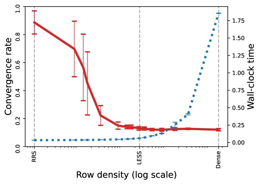
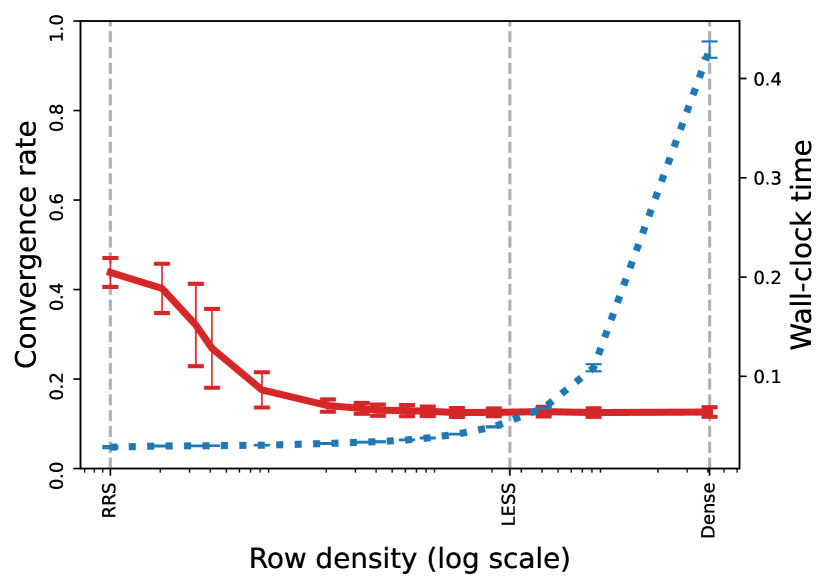
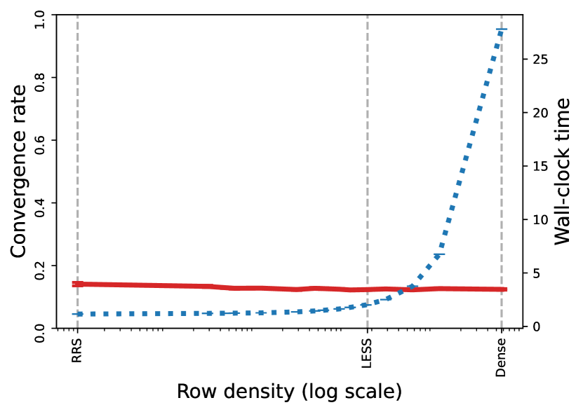
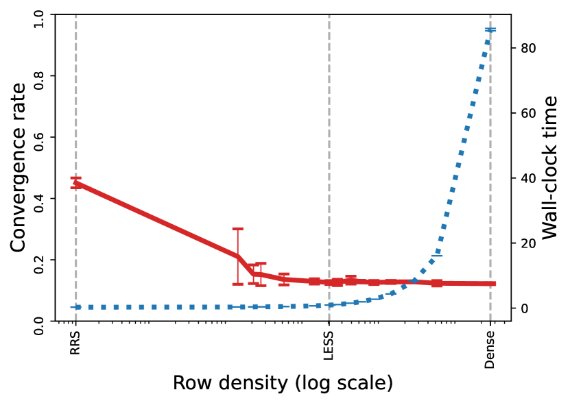
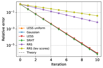
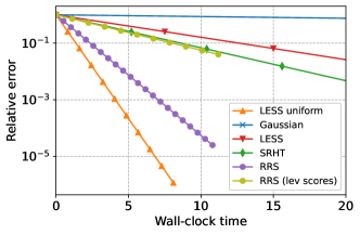
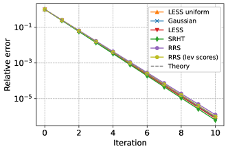
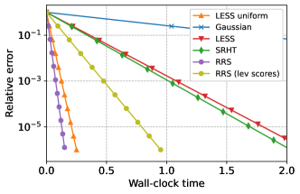
Figure 2: LESS-uniform embeddings: convergence rate of the Newton Sketch for least squares regression and wall-clock time of forming 𝐒𝐀𝐒𝐀\mathbf{S}\mathbf{A} versus row density, with sketch size m=8d𝑚8𝑑m=8d. The results were averaged over 100100100 trials and error bars show twice the empirical standard deviation.

5 Numerical Experiments

We have evaluated our theory on a range of different problems, and we have found that the more precise analysis that our theory provides describes well the convergence behavior for a range of optimization problems. In this section, we present numerical simulations illustrating this for regularized logistic regression and least squares regression, with different datasets ranging from medium to large scale: the CIFAR-10 dataset, the Musk dataset, and WESAD [SRD+18]. Data preprocessing and implementation details, as well as additional numerical results for least squares and regularized least squares, can be found in Appendix E.
Refer to caption
(a) WESAD dataset
Refer to caption
(b) CIFAR-10 dataset
Refer to caption
(c) Musk dataset
Refer to caption
Refer to caption
Refer to caption
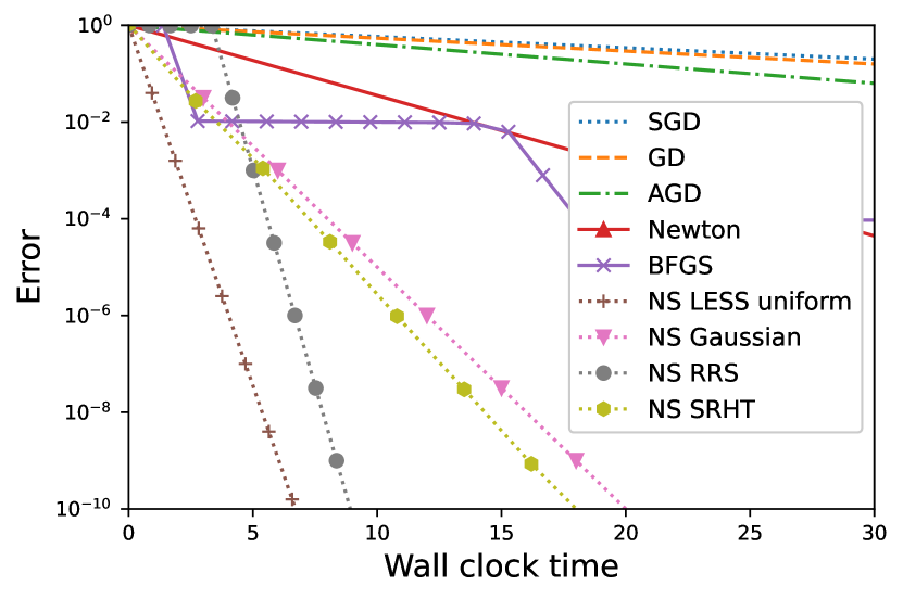
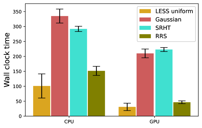
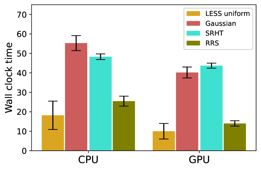
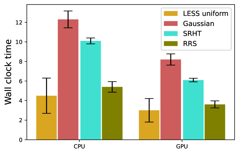
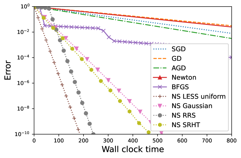
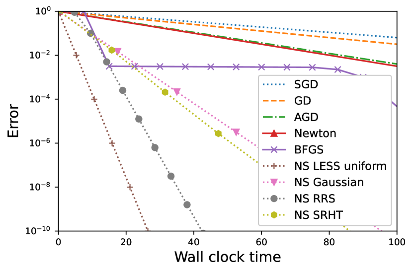
Figure 3: Top plots show the convergence of Newton Sketch (NS) and baselines for logistic regression. We use a sketch size m=d/2𝑚𝑑2m=d/2 for NS. In the bottom plots, we report the CPU and GPU wall-clock times to reach a 106superscript10610^{-6} accurate solution for NS with different sketching methods.

We investigate first the effect of the row density of a LESS-uniform embedding on the Newton Sketch convergence rate and on the time for computing the sketch 𝐒𝐀𝐒𝐀\mathbf{S}\mathbf{A} for least squares regression. In Figure 2, we report these two performance measures versus the row density. (This is the empirical analog for real data of Figure 1). Note that here we also consider a synthetic data matrix with high-coherence, which aims to be more challenging for a uniform sparsifier. Remarkably, our prescribed row density of d𝑑d non-zeros per row offers an excellent empirical trade-off: except for the CIFAR-10 dataset, for which random row sampling performs equally well to Gaussian embeddings, we observe that one can drastically decrease the row density without significantly impairing the convergence rate.

Next, in Figure 3, we investigate a minimization task for the regularized logistic regression loss. Namely, given a data matrix 𝐀n×d𝐀superscript𝑛𝑑\mathbf{A}\in\mathbb{R}^{n\times d} with rows denoted by 𝐚isubscript𝐚𝑖\mathbf{a}_{i}, a target vector of labels 𝐛{±1}n𝐛superscriptplus-or-minus1𝑛\mathbf{b}\in\{\pm 1\}^{n} and a regularization parameter λ>0𝜆0\lambda>0, the goal is to solve:

min𝐱d1ni=1nlog(1+exp(bi𝐚i𝐱))+λ2𝐱22.subscript𝐱superscript𝑑1𝑛superscriptsubscript𝑖1𝑛1subscript𝑏𝑖superscriptsubscript𝐚𝑖top𝐱𝜆2superscriptsubscriptnorm𝐱22\displaystyle\min_{\mathbf{x}\in\mathbb{R}^{d}}\frac{1}{n}\sum_{i=1}^{n}\log(1+\exp(-b_{i}\mathbf{a}_{i}^{\scriptscriptstyle{\top}}\mathbf{x}))+\frac{\lambda}{2}\|\mathbf{x}\|_{2}^{2}\,.

For CIFAR-10 and Musk, we pick λ=104𝜆superscript104\lambda=10^{-4}. For WESAD, we pick λ=105𝜆superscript105\lambda=10^{-5}. We plot the error versus wall-clock time for the Newton Sketch with LESS-uniform, Gaussian embedings, Subsampled Randomized Hadamard Transform (SRHT) and Random Row Sampling (RRS) matrices, for logistic regression, and we compare it with two standard second-order optimization baselines: Newton’s method and BFGS. We also included three first-order baselines: Gradient Descent (GD), Accelerated GD (AGD), and Stochastic GD (SGD), observing much worse performance. Based on the top plots in Figure 3, we conclude that Newton-LESS (i.e., NS LESS uniform) offers significant time speed-ups over all baselines.

Finally, we compare wall-clock time on different hardwares (CPU versus GPU) for the Newton Sketch to reach a 106superscript10610^{-6}-accurate solution (see Appendix E for hardware details). From Figure 3 (bottom plots), we conclude the following: first, when switching from CPU to GPU for WESAD and CIFAR-10, Gaussian embeddings become more efficient than SRHT, despite a worse time complexity, by taking better advantage of the massively parallel architecture; second, Random Row Sampling performs better than either of them, despite having much weaker theoretical guarantees; and third, LESS-uniform is more efficient than all three other methods, on both CPU and GPU hardware platforms, observing a significant speed-up when switching to the parallel GPU architecture.

6 Conclusions

We showed that, when constructing randomized Hessian estimates for second-order optimization, we can get the best of both worlds: the efficiency of Sub-Sampling methods and the precision of Gaussian embeddings, by using sparse sketching matrices known as LEverage Score Sparsified (LESS) embeddings. Our algorithm, called Newton-LESS, enjoys both strong theoretical convergence guarantees and excellent empirical performance on a number of hardware platforms. An important future direction is to explain the surprising effectiveness of the simpler LESS-uniform method, particularly on high-coherence matrices, which goes beyond the predictions of our current theory.

Acknowledgements

We would like to acknowledge DARPA, IARPA, NSF, and ONR via its BRC on RandNLA for providing partial support of this work. Our conclusions do not necessarily reflect the position or the policy of our sponsors, and no official endorsement should be inferred.

References

  • [ABH17] Naman Agarwal, Brian Bullins, and Elad Hazan. Second-order stochastic optimization for machine learning in linear time. Journal of Machine Learning Research, 18(116):1–40, 2017.
  • [AC09] Nir Ailon and Bernard Chazelle. The fast Johnson–Lindenstrauss transform and approximate nearest neighbors. SIAM Journal on computing, 39(1):302–322, 2009.
  • [ACW16] Haim Avron, Kenneth L Clarkson, and David P Woodruff. Sharper bounds for regularized data fitting. arXiv preprint arXiv:1611.03225, 2016.
  • [AM15] Ahmed El Alaoui and Michael W. Mahoney. Fast randomized kernel ridge regression with statistical guarantees. In Proceedings of the 28th International Conference on Neural Information Processing Systems, pages 775–783, December 2015.
  • [AMT10] Haim Avron, Petar Maymounkov, and Sivan Toledo. Blendenpik: Supercharging lapack’s least-squares solver. SIAM Journal on Scientific Computing, 32(3):1217–1236, 2010.
  • [BCNN11] Richard H Byrd, Gillian M Chin, Will Neveitt, and Jorge Nocedal. On the use of stochastic hessian information in optimization methods for machine learning. SIAM Journal on Optimization, 21(3):977–995, 2011.
  • [BCNW12] Richard H Byrd, Gillian M Chin, Jorge Nocedal, and Yuchen Wu. Sample size selection in optimization methods for machine learning. Mathematical programming, 134(1):127–155, 2012.
  • [BS10] Zhidong Bai and Jack W Silverstein. Spectral analysis of large dimensional random matrices, volume 20. Springer, 2010.
  • [BV04] Stephen Boyd and Lieven Vandenberghe. Convex optimization. Cambridge university press, 2004.
  • [CD11] Romain Couillet and Mrouane Debbah. Random Matrix Methods for Wireless Communications. Cambridge University Press, USA, 2011.
  • [CEM+15] Michael B Cohen, Sam Elder, Cameron Musco, Christopher Musco, and Madalina Persu. Dimensionality reduction for k-means clustering and low rank approximation. In Proceedings of the forty-seventh annual ACM symposium on Theory of computing, pages 163–172, 2015.
  • [Coh16] Michael B Cohen. Nearly tight oblivious subspace embeddings by trace inequalities. In Proceedings of the twenty-seventh annual ACM-SIAM symposium on Discrete algorithms, pages 278–287. SIAM, 2016.
  • [CW17] Kenneth L. Clarkson and David P. Woodruff. Low-rank approximation and regression in input sparsity time. J. ACM, 63(6):54:1–54:45, January 2017.
  • [DBPM20] Michał Dereziński, Burak Bartan, Mert Pilanci, and Michael W Mahoney. Debiasing distributed second order optimization with surrogate sketching and scaled regularization. In Advances in Neural Information Processing Systems, volume 33, pages 6889–6899, 2020.
  • [DCV19] Michał Dereziński, Daniele Calandriello, and Michal Valko. Exact sampling of determinantal point processes with sublinear time preprocessing. In H. Wallach, H. Larochelle, A. Beygelzimer, F. d Alché-Buc, E. Fox, and R. Garnett, editors, Advances in Neural Information Processing Systems 32, pages 11542–11554. 2019.
  • [Der19] Michał Dereziński. Fast determinantal point processes via distortion-free intermediate sampling. In Proceedings of the 32nd Conference on Learning Theory, 2019.
  • [DLDM21] Michał Dereziński, Zhenyu Liao, Edgar Dobriban, and Michael W Mahoney. Sparse sketches with small inversion bias. In Proceedings of the 34th Conference on Learning Theory, 2021.
  • [DLLM20] Michał Dereziński, Feynman Liang, Zhenyu Liao, and Michael W Mahoney. Precise expressions for random projections: Low-rank approximation and randomized Newton. In Advances in Neural Information Processing Systems, volume 33, pages 18272–18283, 2020.
  • [DM16] Petros Drineas and Michael W. Mahoney. RandNLA: Randomized numerical linear algebra. Communications of the ACM, 59:80–90, 2016.
  • [DM18] P. Drineas and M. W. Mahoney. Lectures on randomized numerical linear algebra. In M. W. Mahoney, J. C. Duchi, and A. C. Gilbert, editors, The Mathematics of Data, IAS/Park City Mathematics Series, pages 1–48. AMS/IAS/SIAM, 2018.
  • [DM19] Michał Dereziński and Michael W Mahoney. Distributed estimation of the inverse hessian by determinantal averaging. In Advances in Neural Information Processing Systems 32, pages 11401–11411. Curran Associates, Inc., 2019.
  • [DM21] Michał Dereziński and Michael W Mahoney. Determinantal point processes in randomized numerical linear algebra. Notices of the American Mathematical Society, 68(1):34–45, 2021.
  • [DMIMW12a] Petros Drineas, Malik Magdon-Ismail, Michael W. Mahoney, and David P. Woodruff. Fast approximation of matrix coherence and statistical leverage. J. Mach. Learn. Res., 13(1):3475–3506, December 2012.
  • [DMIMW12b] Petros Drineas, Malik Magdon-Ismail, Michael W Mahoney, and David P Woodruff. Fast approximation of matrix coherence and statistical leverage. The Journal of Machine Learning Research, 13(1):3475–3506, 2012.
  • [DMM06] Petros Drineas, Michael W Mahoney, and S Muthukrishnan. Sampling algorithms for 2subscript2\ell_{2} regression and applications. In Proceedings of the seventeenth annual ACM-SIAM symposium on Discrete algorithm, pages 1127–1136, 2006.
  • [DMM08] Petros Drineas, Michael W. Mahoney, and S. Muthukrishnan. Relative-error CUR matrix decompositions. SIAM J. Matrix Anal. Appl., 30(2):844–881, September 2008.
  • [EM15] Murat A Erdogdu and Andrea Montanari. Convergence rates of sub-sampled Newton methods. Advances in Neural Information Processing Systems, 28:3052–3060, 2015.
  • [GGD+21] Vipul Gupta, Avishek Ghosh, Michał Dereziński, Rajiv Khanna, Kannan Ramchandran, and Michael Mahoney. LocalNewton: Reducing communication bottleneck for distributed learning. arXiv preprint arXiv:2105.07320, 2021.
  • [KL17] Vladimir Koltchinskii and Karim Lounici. Concentration inequalities and moment bounds for sample covariance operators. Bernoulli, 23(1):110–133, 2017.
  • [LLDP20] Jonathan Lacotte, Sifan Liu, Edgar Dobriban, and Mert Pilanci. Limiting spectrum of randomized Hadamard transform and optimal iterative sketching methods. In Conference on Neural Information Processing Systems, 2020.
  • [LP19] Jonathan Lacotte and Mert Pilanci. Faster least squares optimization. arXiv preprint arXiv:1911.02675, 2019.
  • [MM13] Xiangrui Meng and Michael W. Mahoney. Low-distortion subspace embeddings in input-sparsity time and applications to robust linear regression. In Proceedings of the Forty-fifth Annual ACM Symposium on Theory of Computing, STOC ’13, pages 91–100, New York, NY, USA, 2013. ACM.
  • [MSM14] Xiangrui Meng, Michael A Saunders, and Michael W Mahoney. LSRN: A parallel iterative solver for strongly over-or underdetermined systems. SIAM Journal on Scientific Computing, 36(2):C95–C118, 2014.
  • [MZ20] Shahar Mendelson and Nikita Zhivotovskiy. Robust covariance estimation under L4L2subscript𝐿4subscript𝐿2{L}_{4}-{L}_{2} norm equivalence. Annals of Statistics, 48(3):1648–1664, 2020.
  • [NN13] Jelani Nelson and Huy L Nguyên. Osnap: Faster numerical linear algebra algorithms via sparser subspace embeddings. In 2013 ieee 54th annual symposium on foundations of computer science, pages 117–126. IEEE, 2013.
  • [PW17] Mert Pilanci and Martin J Wainwright. Newton sketch: A near linear-time optimization algorithm with linear-quadratic convergence. SIAM Journal on Optimization, 27(1):205–245, 2017.
  • [RKM19] Farbod Roosta-Khorasani and Michael W. Mahoney. Sub-Sampled Newton methods. Math. Program., 174(1–2):293–326, March 2019.
  • [RT08] Vladimir Rokhlin and Mark Tygert. A fast randomized algorithm for overdetermined linear least-squares regression. Proceedings of the National Academy of Sciences, 105(36):13212–13217, 2008.
  • [RV13] Mark Rudelson and Roman Vershynin. Hanson-Wright inequality and sub-gaussian concentration. Electronic Communications in Probability, 18, 2013.
  • [Sar06] Tamas Sarlos. Improved approximation algorithms for large matrices via random projections. In Proceedings of the 47th Annual IEEE Symposium on Foundations of Computer Science, FOCS ’06, pages 143–152, Washington, DC, USA, 2006. IEEE Computer Society.
  • [SRD+18] Philip Schmidt, Attila Reiss, Robert Duerichen, Claus Marberger, and Kristof Van Laerhoven. Introducing wesad, a multimodal dataset for wearable stress and affect detection. In Proceedings of the 20th ACM international conference on multimodal interaction, pages 400–408, 2018.
  • [Tro11] Joel A Tropp. Improved analysis of the subsampled randomized Hadamard transform. Advances in Adaptive Data Analysis, 3(01n02):115–126, 2011.
  • [Tro12] Joel A. Tropp. User-friendly tail bounds for sums of random matrices. Foundations of Computational Mathematics, 12(4):389–434, August 2012.
  • [Tro15] Joel A Tropp. An introduction to matrix concentration inequalities. Foundations and Trends in Machine Learning, 8(1-2):1–230, 2015.
  • [Woo14] David P Woodruff. Sketching as a tool for numerical linear algebra. Foundations and Trends® in Theoretical Computer Science, 10(1–2):1–157, 2014.
  • [WRKXM18] Shusen Wang, Farbod Roosta-Khorasani, Peng Xu, and Michael W Mahoney. GIANT: Globally improved approximate Newton method for distributed optimization. In Advances in Neural Information Processing Systems 31, pages 2332–2342. 2018.
  • [XRKM17] Peng Xu, Farbod Roosta-Khorasani, and Michael Mahoney. Newton-type methods for non-convex optimization under inexact hessian information. Mathematical Programming, August 2017.
  • [YXRKM18] Z. Yao, P. Xu, F. Roosta-Khorasani, and M. W. Mahoney. Inexact non-convex Newton-type methods. Technical report, 2018. Preprint: arXiv:1802.06925.

Appendix A Characterization of Inverse Moments (Proof of Theorem 6)

In this section, we prove Theorem 6. The proof consists of two parts corresponding to the first and second moment of 𝐐𝐐\mathbf{Q}. The analysis of the first moment bound is nearly the same as in [DLDM21], so we only outline it here, highlighting the differences coming from the regularization matrix 𝐂𝐂\mathbf{C}. The analysis of the second moment is our main contribution in this proof, and we discuss it in detail. First, however, we define the high probability event \mathcal{E} which is common to both parts.

To simplify the proof, we will let m𝑚m be divisible by 333. Note that we have 𝐐=(𝐔𝐒𝐒𝐔+𝐃)1𝐐superscriptsuperscript𝐔topsuperscript𝐒top𝐒𝐔𝐃1\mathbf{Q}=(\mathbf{U}^{\scriptscriptstyle{\top}}\mathbf{S}^{\scriptscriptstyle{\top}}\mathbf{S}\mathbf{U}+\mathbf{D})^{-1} for 𝐃=𝐇12𝐂𝐇12𝐃superscript𝐇12superscript𝐂𝐇12\mathbf{D}=\mathbf{H}^{-\frac{1}{2}}\mathbf{C}\mathbf{H}^{-\frac{1}{2}}. Moreover, let 𝐒isubscript𝐒𝑖\mathbf{S}_{-i} denote 𝐒𝐒\mathbf{S} without the i𝑖ith row, and let 𝐐i=(𝐔𝐒i𝐒i𝐔+𝐃)1subscript𝐐𝑖superscriptsuperscript𝐔topsuperscriptsubscript𝐒𝑖topsubscript𝐒𝑖𝐔𝐃1\mathbf{Q}_{-i}=(\mathbf{U}^{\scriptscriptstyle{\top}}\mathbf{S}_{-i}^{\scriptscriptstyle{\top}}\mathbf{S}_{-i}\mathbf{U}+\mathbf{D})^{-1}. Also, define 𝐒~1subscript~𝐒1\widetilde{\mathbf{S}}_{1}, 𝐒~2subscript~𝐒2\widetilde{\mathbf{S}}_{2}, 𝐒~3subscript~𝐒3\widetilde{\mathbf{S}}_{3} as the matrices consisting of the first, second and third group of m/3𝑚3m/3 rows in 𝐒𝐒\mathbf{S}, all scaled by 33\sqrt{3}, so that 𝐒𝐒=13j=13𝐒~j𝐒~jsuperscript𝐒top𝐒13superscriptsubscript𝑗13superscriptsubscript~𝐒𝑗topsubscript~𝐒𝑗\mathbf{S}^{\scriptscriptstyle{\top}}\mathbf{S}=\frac{1}{3}\sum_{j=1}^{3}\widetilde{\mathbf{S}}_{j}^{\scriptscriptstyle{\top}}\widetilde{\mathbf{S}}_{j}. Next, using 𝚺=𝐔𝐔𝚺superscript𝐔top𝐔\mathbf{\Sigma}=\mathbf{U}^{\scriptscriptstyle{\top}}\mathbf{U}, similarly as in [DLDM21] we let t=m/3𝑡𝑚3t=m/3 and define three independent events:

j:𝚺𝐔𝐒~j𝐒~j𝐔η,forj=1,2,3,\displaystyle\mathcal{E}_{j}:\quad\big{\|}\mathbf{\Sigma}-\mathbf{U}^{\scriptscriptstyle{\top}}\widetilde{\mathbf{S}}_{j}^{\scriptscriptstyle{\top}}\widetilde{\mathbf{S}}_{j}\mathbf{U}\big{\|}\leq\eta,\quad\text{for}\quad j=1,2,3, (5)

with =j=13jsuperscriptsubscript𝑗13subscript𝑗\mathcal{E}=\bigwedge_{j=1}^{3}\mathcal{E}_{j} defined as the intersection of the events. Conditioned on \mathcal{E}, we have:

𝐈(𝐔𝐒𝐒𝐔+𝐃)norm𝐈superscript𝐔topsuperscript𝐒top𝐒𝐔𝐃\displaystyle\|\mathbf{I}-(\mathbf{U}^{\scriptscriptstyle{\top}}\mathbf{S}^{\scriptscriptstyle{\top}}\mathbf{S}\mathbf{U}+\mathbf{D})\| =13j=13(𝚺𝐔𝐒~j𝐒~j𝐔)13j=13𝚺𝐔𝐒~j𝐒~j𝐔η,absentnorm13superscriptsubscript𝑗13𝚺superscript𝐔topsuperscriptsubscript~𝐒𝑗topsubscript~𝐒𝑗𝐔13superscriptsubscript𝑗13norm𝚺superscript𝐔topsuperscriptsubscript~𝐒𝑗topsubscript~𝐒𝑗𝐔𝜂\displaystyle=\Big{\|}\frac{1}{3}\sum_{j=1}^{3}\big{(}\mathbf{\Sigma}-\mathbf{U}^{\scriptscriptstyle{\top}}\widetilde{\mathbf{S}}_{j}^{\scriptscriptstyle{\top}}\widetilde{\mathbf{S}}_{j}\mathbf{U}\big{)}\Big{\|}\leq\frac{1}{3}\sum_{j=1}^{3}\|\mathbf{\Sigma}-\mathbf{U}^{\scriptscriptstyle{\top}}\widetilde{\mathbf{S}}_{j}^{\scriptscriptstyle{\top}}\widetilde{\mathbf{S}}_{j}\mathbf{U}\|\leq\eta,

which implies that 𝐐𝐈η1η2ηnorm𝐐𝐈𝜂1𝜂2𝜂\|\mathbf{Q}-\mathbf{I}\|\leq\frac{\eta}{1-\eta}\leq 2\eta. Furthermore, an important property of the definition of \mathcal{E} is that for each i{1,,m}𝑖1𝑚i\in\{1,...,m\} there is a j{1,2,3}𝑗123j\in\{1,2,3\} such that jsubscript𝑗\mathcal{E}_{j} is independent of 𝐱isubscript𝐱𝑖\mathbf{x}_{i}, and after conditioning only on jsubscript𝑗\mathcal{E}_{j} we get 𝐐i6normsubscript𝐐𝑖6\|\mathbf{Q}_{-i}\|\leq 6. From Condition 1 and the union bound we conclude that Pr()1δPr1𝛿\Pr(\mathcal{E})\geq 1-\delta.

The analysis of both the first and second moment uses the Sherman-Morrison formula, to separate one of the rows from the rest of the sketch. We state this formula in the following lemma.

Lemma 12 (Sherman-Morrison).

For 𝐀n×n𝐀superscript𝑛𝑛\mathbf{A}\in\mathbb{R}^{n\times n} invertible and 𝐮,𝐯n𝐮𝐯superscript𝑛\mathbf{u},\mathbf{v}\in\mathbb{R}^{n}, 𝐀+𝐮𝐯𝐀superscript𝐮𝐯top\mathbf{A}+\mathbf{u}\mathbf{v}^{\scriptscriptstyle{\top}} is invertible if and only if 1+𝐯𝐀1𝐮01superscript𝐯topsuperscript𝐀1𝐮01+\mathbf{v}^{\scriptscriptstyle{\top}}\mathbf{A}^{-1}\mathbf{u}\neq 0 and

(𝐀+𝐮𝐯)1=𝐀1𝐀1𝐮𝐯𝐀11+𝐯𝐀1𝐮.superscript𝐀superscript𝐮𝐯top1superscript𝐀1superscript𝐀1superscript𝐮𝐯topsuperscript𝐀11superscript𝐯topsuperscript𝐀1𝐮(\mathbf{A}+\mathbf{u}\mathbf{v}^{\scriptscriptstyle{\top}})^{-1}=\mathbf{A}^{-1}-\frac{\mathbf{A}^{-1}\mathbf{u}\mathbf{v}^{\scriptscriptstyle{\top}}\mathbf{A}^{-1}}{1+\mathbf{v}^{\scriptscriptstyle{\top}}\mathbf{A}^{-1}\mathbf{u}}.

From the above formula, it follows that:

(𝐀+𝐮𝐯)1𝐮=𝐀1𝐮1+𝐯𝐀1𝐮.superscript𝐀superscript𝐮𝐯top1𝐮superscript𝐀1𝐮1superscript𝐯topsuperscript𝐀1𝐮(\mathbf{A}+\mathbf{u}\mathbf{v}^{\scriptscriptstyle{\top}})^{-1}\mathbf{u}=\frac{\mathbf{A}^{-1}\mathbf{u}}{1+\mathbf{v}^{\scriptscriptstyle{\top}}\mathbf{A}^{-1}\mathbf{u}}.

A.1 Proof of first moment bound

In this part of the proof we recall the decomposition of 𝔼[𝐐]subscript𝔼delimited-[]𝐐\mathbb{E}_{\mathcal{E}}[\mathbf{Q}] used by [DLDM21]. Most of their analysis is unaffected by the presence of the regularization matrix 𝐃𝐃\mathbf{D}, so we will focus on the steps that will also be needed for our analysis of the second moment. Let the i𝑖ith row of 𝐒𝐒\mathbf{S} be 1mdeff𝐬i1𝑚subscript𝑑effsuperscriptsubscript𝐬𝑖top\frac{1}{\sqrt{m-{d_{\textnormal{eff}}}}}\mathbf{s}_{i}^{\scriptscriptstyle{\top}}, and define 𝐱i=m𝐔𝐬isubscript𝐱𝑖𝑚superscript𝐔topsubscript𝐬𝑖\mathbf{x}_{i}=m\mathbf{U}^{\scriptscriptstyle{\top}}\mathbf{s}_{i}, so that 𝐔𝐒𝐒𝐔=γmi𝐱i𝐱isuperscript𝐔topsuperscript𝐒top𝐒𝐔𝛾𝑚subscript𝑖subscript𝐱𝑖superscriptsubscript𝐱𝑖top\mathbf{U}^{\scriptscriptstyle{\top}}\mathbf{S}^{\scriptscriptstyle{\top}}\mathbf{S}\mathbf{U}=\frac{\gamma}{m}\sum_{i}\mathbf{x}_{i}\mathbf{x}_{i}^{\scriptscriptstyle{\top}}, where γ=mmdeff𝛾𝑚𝑚subscript𝑑eff\gamma=\frac{m}{m-{d_{\textnormal{eff}}}}. Using γi=1+γm𝐱i𝐐i𝐱isubscript𝛾𝑖1𝛾𝑚superscriptsubscript𝐱𝑖topsubscript𝐐𝑖subscript𝐱𝑖\gamma_{i}=1+\frac{\gamma}{m}\mathbf{x}_{i}^{\scriptscriptstyle{\top}}\mathbf{Q}_{-i}\mathbf{x}_{i}, we have:

𝔼[𝐐]𝐈subscript𝔼delimited-[]𝐐𝐈\displaystyle\mathbb{E}_{\mathcal{E}}[\mathbf{Q}]-\mathbf{I} =𝔼[𝐐(𝚺+𝐃)𝐐(𝐔𝐒𝐒𝐔+𝐃)]absentsubscript𝔼delimited-[]𝐐𝚺𝐃𝐐superscript𝐔topsuperscript𝐒top𝐒𝐔𝐃\displaystyle=\mathbb{E}_{\mathcal{E}}[\mathbf{Q}(\mathbf{\Sigma}+\mathbf{D})-\mathbf{Q}(\mathbf{U}^{\scriptscriptstyle{\top}}\mathbf{S}^{\scriptscriptstyle{\top}}\mathbf{S}\mathbf{U}+\mathbf{D})]
=𝔼[𝐐𝚺]𝔼[𝐐𝐔𝐒𝐒𝐔]absentsubscript𝔼delimited-[]𝐐𝚺subscript𝔼delimited-[]superscript𝐐𝐔topsuperscript𝐒top𝐒𝐔\displaystyle=\mathbb{E}_{\mathcal{E}}[\mathbf{Q}\mathbf{\Sigma}]-\mathbb{E}_{\mathcal{E}}[\mathbf{Q}\mathbf{U}^{\scriptscriptstyle{\top}}\mathbf{S}^{\scriptscriptstyle{\top}}\mathbf{S}\mathbf{U}]
=()𝔼[𝐐𝚺]𝔼[γγi𝐐i𝐱i𝐱i]subscript𝔼delimited-[]𝐐𝚺subscript𝔼delimited-[]𝛾subscript𝛾𝑖subscript𝐐𝑖subscript𝐱𝑖superscriptsubscript𝐱𝑖top\displaystyle\overset{(*)}{=}\mathbb{E}_{\mathcal{E}}[\mathbf{Q}\mathbf{\Sigma}]-\mathbb{E}_{\mathcal{E}}[\tfrac{\gamma}{\gamma_{i}}\mathbf{Q}_{-i}\mathbf{x}_{i}\mathbf{x}_{i}^{\scriptscriptstyle{\top}}]
=𝔼[𝐐𝐐i]𝚺+𝔼[𝐐i(𝚺𝐱i𝐱i)]+𝔼[(1γγi)𝐐i𝐱i𝐱i],absentsubscript𝔼delimited-[]𝐐subscript𝐐𝑖𝚺subscript𝔼delimited-[]subscript𝐐𝑖𝚺subscript𝐱𝑖superscriptsubscript𝐱𝑖topsubscript𝔼delimited-[]1𝛾subscript𝛾𝑖subscript𝐐𝑖subscript𝐱𝑖superscriptsubscript𝐱𝑖top\displaystyle=\mathbb{E}_{\mathcal{E}}[\mathbf{Q}-\mathbf{Q}_{-i}]\mathbf{\Sigma}+\mathbb{E}_{\mathcal{E}}[\mathbf{Q}_{-i}(\mathbf{\Sigma}-\mathbf{x}_{i}\mathbf{x}_{i}^{\scriptscriptstyle{\top}})]+\mathbb{E}_{\mathcal{E}}[(1-\tfrac{\gamma}{\gamma_{i}})\mathbf{Q}_{-i}\mathbf{x}_{i}\mathbf{x}_{i}^{\scriptscriptstyle{\top}}],

where ()(*) follows from the Sherman-Morrison formula. From this point, the analysis of [DLDM21] proceeds to bound the spectral norm of the first two terms by O(1/m)𝑂1𝑚O(1/m), and the spectral norm of the last term by O(tr(𝐔𝐔)/m)𝑂trsuperscript𝐔top𝐔𝑚O(\sqrt{\mathrm{tr}(\mathbf{U}^{\scriptscriptstyle{\top}}\mathbf{U})}/m). In their setup, 𝐂=𝟎𝐂0\mathbf{C}=\mathbf{0}, which means that tr(𝐔𝐔)=dtrsuperscript𝐔top𝐔𝑑\mathrm{tr}(\mathbf{U}^{\scriptscriptstyle{\top}}\mathbf{U})=d, whereas in our more general statement, we let deff=tr(𝐔𝐔)subscript𝑑efftrsuperscript𝐔top𝐔{d_{\textnormal{eff}}}=\mathrm{tr}(\mathbf{U}^{\scriptscriptstyle{\top}}\mathbf{U}). This does not affect the proofs. For the sake of our analysis of the second moment, we separate out the following guarantees obtained by [DLDM21], given here in a slightly more general form than originally.

Lemma 13 ([DLDM21]).

The following bounds hold for k{1,2}𝑘12k\in\{1,2\}:

𝔼[𝐐k𝐐ik]𝚺normsubscript𝔼delimited-[]superscript𝐐𝑘superscriptsubscript𝐐𝑖𝑘𝚺\displaystyle\|\mathbb{E}_{\mathcal{E}}[\mathbf{Q}^{k}-\mathbf{Q}_{-i}^{k}]\mathbf{\Sigma}\| =O(1/m),absent𝑂1𝑚\displaystyle=O(1/m),
𝔼[𝐐ik(𝐱i𝐱i𝚺)]normsubscript𝔼delimited-[]superscriptsubscript𝐐𝑖𝑘subscript𝐱𝑖superscriptsubscript𝐱𝑖top𝚺\displaystyle\|\mathbb{E}_{\mathcal{E}}[\mathbf{Q}_{-i}^{k}(\mathbf{x}_{i}\mathbf{x}_{i}^{\scriptscriptstyle{\top}}-\mathbf{\Sigma})]\| =O(1/m),absent𝑂1𝑚\displaystyle=O(1/m),
𝔼[(γγi1)𝐐ik𝐱i𝐱i]normsubscript𝔼delimited-[]𝛾subscript𝛾𝑖1superscriptsubscript𝐐𝑖𝑘subscript𝐱𝑖superscriptsubscript𝐱𝑖top\displaystyle\|\mathbb{E}_{\mathcal{E}}[(\tfrac{\gamma}{\gamma_{i}}-1)\mathbf{Q}_{-i}^{k}\mathbf{x}_{i}\mathbf{x}_{i}^{\scriptscriptstyle{\top}}]\| =O(deff/m).absent𝑂subscript𝑑eff𝑚\displaystyle=O(\sqrt{d_{\textnormal{eff}}}/m).

A.2 Proof of second moment bound

We next present the analysis of the second moment, 𝔼[𝐐2]subscript𝔼delimited-[]superscript𝐐2\mathbb{E}_{\mathcal{E}}[\mathbf{Q}^{2}], which requires a considerably more elaborate decomposition. Using ρ=deffmd~eff𝜌subscript𝑑eff𝑚subscript~𝑑eff\rho=\frac{{d_{\textnormal{eff}}}}{m-{\tilde{d}_{\textnormal{eff}}}} and 𝚺=𝐔𝐔𝚺superscript𝐔top𝐔\mathbf{\Sigma}=\mathbf{U}^{\scriptscriptstyle{\top}}\mathbf{U}, we have:

𝔼[𝐐2](𝐈+ρ𝚺)=(𝔼[𝐐]𝐈)𝐓1+(𝔼[𝐐(𝐐𝐈)]ρ𝚺).subscript𝔼delimited-[]superscript𝐐2𝐈𝜌𝚺subscriptsubscript𝔼delimited-[]𝐐𝐈subscript𝐓1subscript𝔼delimited-[]𝐐𝐐𝐈𝜌𝚺\displaystyle\mathbb{E}_{\mathcal{E}}[\mathbf{Q}^{2}]-(\mathbf{I}+\rho\mathbf{\Sigma})=\underbrace{\big{(}\mathbb{E}_{\mathcal{E}}[\mathbf{Q}]-\mathbf{I}\big{)}}_{\mathbf{T}_{1}}+\big{(}\mathbb{E}_{\mathcal{E}}[\mathbf{Q}(\mathbf{Q}-\mathbf{I})]-\rho\mathbf{\Sigma}\big{)}.

Recalling that 𝚺+𝐃=𝐈𝚺𝐃𝐈\mathbf{\Sigma}+\mathbf{D}=\mathbf{I}, we can rewrite the last term as:

𝔼[𝐐(𝐐𝐈)]subscript𝔼delimited-[]𝐐𝐐𝐈\displaystyle\mathbb{E}_{\mathcal{E}}[\mathbf{Q}(\mathbf{Q}-\mathbf{I})] =𝔼[𝐐(𝐐(𝚺+𝐃)𝐐(𝐔𝐒𝐒𝐔+𝐃))]absentsubscript𝔼delimited-[]𝐐𝐐𝚺𝐃𝐐superscript𝐔topsuperscript𝐒top𝐒𝐔𝐃\displaystyle=\mathbb{E}_{\mathcal{E}}[\mathbf{Q}(\mathbf{Q}(\mathbf{\Sigma}+\mathbf{D})-\mathbf{Q}(\mathbf{U}^{\scriptscriptstyle{\top}}\mathbf{S}^{\scriptscriptstyle{\top}}\mathbf{S}\mathbf{U}+\mathbf{D}))]
=𝔼[𝐐(𝐐𝚺𝐐𝐔𝐒𝐒𝐔)]absentsubscript𝔼delimited-[]𝐐𝐐𝚺superscript𝐐𝐔topsuperscript𝐒top𝐒𝐔\displaystyle=\mathbb{E}_{\mathcal{E}}[\mathbf{Q}(\mathbf{Q}\mathbf{\Sigma}-\mathbf{Q}\mathbf{U}^{\scriptscriptstyle{\top}}\mathbf{S}^{\scriptscriptstyle{\top}}\mathbf{S}\mathbf{U})]
=(a)𝔼[𝐐(𝐐𝚺γγi𝐐i𝐱i𝐱i)]𝑎subscript𝔼delimited-[]𝐐𝐐𝚺𝛾subscript𝛾𝑖subscript𝐐𝑖subscript𝐱𝑖superscriptsubscript𝐱𝑖top\displaystyle\overset{(a)}{=}\mathbb{E}_{\mathcal{E}}[\mathbf{Q}(\mathbf{Q}\mathbf{\Sigma}-\tfrac{\gamma}{\gamma_{i}}\mathbf{Q}_{-i}\mathbf{x}_{i}\mathbf{x}_{i}^{\scriptscriptstyle{\top}})]
=(b)𝔼[𝐐2]𝚺𝔼[γγi𝐐i2𝐱i𝐱i]+𝔼[𝐱i𝐐i2𝐱imγ2γi2𝐐i𝐱i𝐱i]𝑏subscript𝔼delimited-[]superscript𝐐2𝚺subscript𝔼delimited-[]𝛾subscript𝛾𝑖superscriptsubscript𝐐𝑖2subscript𝐱𝑖superscriptsubscript𝐱𝑖topsubscript𝔼delimited-[]superscriptsubscript𝐱𝑖topsuperscriptsubscript𝐐𝑖2subscript𝐱𝑖𝑚superscript𝛾2superscriptsubscript𝛾𝑖2subscript𝐐𝑖subscript𝐱𝑖superscriptsubscript𝐱𝑖top\displaystyle\overset{(b)}{=}\mathbb{E}_{\mathcal{E}}[\mathbf{Q}^{2}]\mathbf{\Sigma}-\mathbb{E}_{\mathcal{E}}[\tfrac{\gamma}{\gamma_{i}}\mathbf{Q}_{-i}^{2}\mathbf{x}_{i}\mathbf{x}_{i}^{\scriptscriptstyle{\top}}]+\mathbb{E}_{\mathcal{E}}\Big{[}\tfrac{\mathbf{x}_{i}^{\scriptscriptstyle{\top}}\mathbf{Q}_{-i}^{2}\mathbf{x}_{i}}{m}\,\tfrac{\gamma^{2}}{\gamma_{i}^{2}}\mathbf{Q}_{-i}\mathbf{x}_{i}\mathbf{x}_{i}^{\scriptscriptstyle{\top}}\Big{]}
=𝔼[𝐐2𝐐i2]𝚺𝐓2+𝔼[𝐐i2(𝚺𝐱i𝐱i)]𝐓3+𝔼[(1γγi)𝐐i2𝐱i𝐱i]𝐓4+𝔼[𝐱i𝐐i2𝐱imγ2γi2𝐐i𝐱i𝐱i],absentsubscriptsubscript𝔼delimited-[]superscript𝐐2superscriptsubscript𝐐𝑖2𝚺subscript𝐓2subscriptsubscript𝔼delimited-[]superscriptsubscript𝐐𝑖2𝚺subscript𝐱𝑖superscriptsubscript𝐱𝑖topsubscript𝐓3subscriptsubscript𝔼delimited-[]1𝛾subscript𝛾𝑖superscriptsubscript𝐐𝑖2subscript𝐱𝑖superscriptsubscript𝐱𝑖topsubscript𝐓4subscript𝔼delimited-[]superscriptsubscript𝐱𝑖topsuperscriptsubscript𝐐𝑖2subscript𝐱𝑖𝑚superscript𝛾2superscriptsubscript𝛾𝑖2subscript𝐐𝑖subscript𝐱𝑖superscriptsubscript𝐱𝑖top\displaystyle=\underbrace{\mathbb{E}_{\mathcal{E}}[\mathbf{Q}^{2}-\mathbf{Q}_{-i}^{2}]\mathbf{\Sigma}}_{\mathbf{T}_{2}}+\underbrace{\mathbb{E}_{\mathcal{E}}[\mathbf{Q}_{-i}^{2}(\mathbf{\Sigma}-\mathbf{x}_{i}\mathbf{x}_{i}^{\scriptscriptstyle{\top}})]}_{\mathbf{T}_{3}}+\underbrace{\mathbb{E}_{\mathcal{E}}[(1-\tfrac{\gamma}{\gamma_{i}})\mathbf{Q}_{-i}^{2}\mathbf{x}_{i}\mathbf{x}_{i}^{\scriptscriptstyle{\top}}]}_{\mathbf{T}_{4}}+\mathbb{E}_{\mathcal{E}}\Big{[}\tfrac{\mathbf{x}_{i}^{\scriptscriptstyle{\top}}\mathbf{Q}_{-i}^{2}\mathbf{x}_{i}}{m}\,\tfrac{\gamma^{2}}{\gamma_{i}^{2}}\mathbf{Q}_{-i}\mathbf{x}_{i}\mathbf{x}_{i}^{\scriptscriptstyle{\top}}\Big{]},

for a fixed i𝑖i, where we denote γi=1+γm𝐱i𝐐i𝐱isubscript𝛾𝑖1𝛾𝑚superscriptsubscript𝐱𝑖topsubscript𝐐𝑖subscript𝐱𝑖\gamma_{i}=1+\frac{\gamma}{m}\mathbf{x}_{i}^{\scriptscriptstyle{\top}}\mathbf{Q}_{-i}\mathbf{x}_{i}. Note that we used the Sherman-Morrison formula twice, in steps (a)𝑎(a) and (b)𝑏(b). We can put everything together as follows:

𝔼[𝐐2](𝐈+ρ𝚺)subscript𝔼delimited-[]superscript𝐐2𝐈𝜌𝚺\displaystyle\mathbb{E}_{\mathcal{E}}[\mathbf{Q}^{2}]-(\mathbf{I}+\rho\mathbf{\Sigma}) =𝐓1+𝐓2+𝐓3+𝐓4absentsubscript𝐓1subscript𝐓2subscript𝐓3subscript𝐓4\displaystyle=\mathbf{T}_{1}+\mathbf{T}_{2}+\mathbf{T}_{3}+\mathbf{T}_{4}
+ρ(𝔼[𝐐i]𝐈)𝚺𝐓5+ρ𝔼[𝐐i(𝐱i𝐱i𝚺)]𝐓6+𝔼[(𝐱i𝐐i2𝐱imγ2γi2ρ)𝐐i𝐱i𝐱i]𝐓7.subscript𝜌subscript𝔼delimited-[]subscript𝐐𝑖𝐈𝚺subscript𝐓5subscript𝜌subscript𝔼delimited-[]subscript𝐐𝑖subscript𝐱𝑖superscriptsubscript𝐱𝑖top𝚺subscript𝐓6subscriptsubscript𝔼delimited-[]superscriptsubscript𝐱𝑖topsuperscriptsubscript𝐐𝑖2subscript𝐱𝑖𝑚superscript𝛾2superscriptsubscript𝛾𝑖2𝜌subscript𝐐𝑖subscript𝐱𝑖superscriptsubscript𝐱𝑖topsubscript𝐓7\displaystyle+\underbrace{\rho(\mathbb{E}_{\mathcal{E}}[\mathbf{Q}_{-i}]-\mathbf{I})\mathbf{\Sigma}}_{\mathbf{T}_{5}}+\underbrace{\rho\,\mathbb{E}_{\mathcal{E}}[\mathbf{Q}_{-i}(\mathbf{x}_{i}\mathbf{x}_{i}^{\scriptscriptstyle{\top}}-\mathbf{\Sigma})]}_{\mathbf{T}_{6}}+\underbrace{\mathbb{E}_{\mathcal{E}}\Big{[}\Big{(}\tfrac{\mathbf{x}_{i}^{\scriptscriptstyle{\top}}\mathbf{Q}_{-i}^{2}\mathbf{x}_{i}}{m}\,\tfrac{\gamma^{2}}{\gamma_{i}^{2}}-\rho\Big{)}\mathbf{Q}_{-i}\mathbf{x}_{i}\mathbf{x}_{i}^{\scriptscriptstyle{\top}}\Big{]}}_{\mathbf{T}_{7}}.

From the bound on the first moment of 𝐐𝐐\mathbf{Q}, we conclude that 𝐓1=O(deff/m)normsubscript𝐓1𝑂subscript𝑑eff𝑚\|\mathbf{T}_{1}\|=O(\sqrt{d_{\textnormal{eff}}}/m) and that 𝐓5=O(deff/m)normsubscript𝐓5𝑂subscript𝑑eff𝑚\|\mathbf{T}_{5}\|=O(\sqrt{d_{\textnormal{eff}}}/m). Without loss of generality, assume that events 1subscript1\mathcal{E}_{1} and 2subscript2\mathcal{E}_{2} are both independent of 𝐱isubscript𝐱𝑖\mathbf{x}_{i}, and let =12superscriptsubscript1subscript2\mathcal{E}^{\prime}=\mathcal{E}_{1}\wedge\mathcal{E}_{2} as well as δ3=Pr(¬3)subscript𝛿3Prsubscript3\delta_{3}=\Pr(\neg\mathcal{E}_{3}). Next, we will use the fact that for a p.s.d. random matrix 𝐌𝐌\mathbf{M} in the probability space of 𝐒𝐒\mathbf{S}, we have 𝔼[𝐌]11δ𝔼[𝐌]2𝔼[𝐌]precedes-or-equalssubscript𝔼delimited-[]𝐌11𝛿subscript𝔼superscriptdelimited-[]𝐌precedes-or-equals2subscript𝔼superscriptdelimited-[]𝐌\mathbb{E}_{\mathcal{E}}[\mathbf{M}]\preceq\frac{1}{1-\delta}\mathbb{E}_{\mathcal{E}^{\prime}}[\mathbf{M}]\preceq 2\cdot\mathbb{E}_{\mathcal{E}^{\prime}}[\mathbf{M}].

Using k=2𝑘2k=2 in Lemma 13, we can bound 𝐓2normsubscript𝐓2\|\mathbf{T}_{2}\|, 𝐓3normsubscript𝐓3\|\mathbf{T}_{3}\| and 𝐓4normsubscript𝐓4\|\mathbf{T}_{4}\| by O(deff/m)𝑂subscript𝑑eff𝑚O(\sqrt{d_{\textnormal{eff}}}/m), and setting k=1𝑘1k=1, we can do the same for 𝐓6normsubscript𝐓6\|\mathbf{T}_{6}\|.

Thus, it remains to bound 𝐓7normsubscript𝐓7\|\mathbf{T}_{7}\|. Let γ~=mmd~eff~𝛾𝑚𝑚subscript~𝑑eff{\tilde{\gamma}}=\frac{m}{m-{\tilde{d}_{\textnormal{eff}}}}. We first use the Cauchy-Schwartz inequality twice, obtaining that:

𝐓71m𝔼[(γ~deff𝐱i𝐐i2𝐱iγ2γi2)2]sup𝐮=1𝔼[(𝐮𝐐i𝐱i)4]4sup𝐮=1𝔼[(𝐱i𝐮)4]4.normsubscript𝐓71𝑚subscript𝔼delimited-[]superscript~𝛾subscript𝑑effsuperscriptsubscript𝐱𝑖topsuperscriptsubscript𝐐𝑖2subscript𝐱𝑖superscript𝛾2superscriptsubscript𝛾𝑖22subscriptsupremumnorm𝐮14subscript𝔼delimited-[]superscriptsuperscript𝐮topsubscript𝐐𝑖subscript𝐱𝑖4subscriptsupremumnorm𝐮14subscript𝔼delimited-[]superscriptsuperscriptsubscript𝐱𝑖top𝐮4\displaystyle\|\mathbf{T}_{7}\|\leq\frac{1}{m}\sqrt{\mathbb{E}_{\mathcal{E}}\Big{[}\Big{(}{\tilde{\gamma}}{d_{\textnormal{eff}}}-\mathbf{x}_{i}^{\scriptscriptstyle{\top}}\mathbf{Q}_{-i}^{2}\mathbf{x}_{i}\cdot\tfrac{\gamma^{2}}{\gamma_{i}^{2}}\Big{)}^{2}\Big{]}}\cdot\sup_{\|\mathbf{u}\|=1}\sqrt[4]{\mathbb{E}_{\mathcal{E}}\big{[}(\mathbf{u}^{\scriptscriptstyle{\top}}\mathbf{Q}_{-i}\mathbf{x}_{i})^{4}\big{]}}\cdot\sup_{\|\mathbf{u}\|=1}\sqrt[4]{\mathbb{E}_{\mathcal{E}}\big{[}(\mathbf{x}_{i}^{\scriptscriptstyle{\top}}\mathbf{u})^{4}\big{]}}. (6)

The latter two terms can each be bounded easily by O(α+14)𝑂4𝛼1O(\sqrt[4]{\alpha+1}) using Condition 2. For instance, considering the middle term, we have:

𝔼[(𝐮𝐐i𝐱i)4]subscript𝔼delimited-[]superscriptsuperscript𝐮topsubscript𝐐𝑖subscript𝐱𝑖4\displaystyle\mathbb{E}_{\mathcal{E}}\big{[}(\mathbf{u}^{\scriptscriptstyle{\top}}\mathbf{Q}_{-i}\mathbf{x}_{i})^{4}\big{]} 2𝔼[𝔼[(𝐱i𝐐i𝐮𝐮𝐐i𝐱i)2𝐐i]]absent2subscript𝔼superscriptdelimited-[]𝔼delimited-[]conditionalsuperscriptsuperscriptsubscript𝐱𝑖topsubscript𝐐𝑖superscript𝐮𝐮topsubscript𝐐𝑖subscript𝐱𝑖2subscript𝐐𝑖\displaystyle\leq 2\,\mathbb{E}_{\mathcal{E}^{\prime}}\Big{[}\mathbb{E}\big{[}(\mathbf{x}_{i}^{\scriptscriptstyle{\top}}\mathbf{Q}_{-i}\mathbf{u}\mathbf{u}^{\scriptscriptstyle{\top}}\mathbf{Q}_{-i}\mathbf{x}_{i})^{2}\mid\mathbf{Q}_{-i}\big{]}\Big{]}
=2𝔼[Var[𝐱i𝐐i𝐮𝐮𝐐i𝐱i𝐐i]+(𝔼[𝐱i𝐐i𝐮𝐮𝐐i𝐱i𝐐i])2]absent2subscript𝔼superscriptdelimited-[]Vardelimited-[]conditionalsuperscriptsubscript𝐱𝑖topsubscript𝐐𝑖superscript𝐮𝐮topsubscript𝐐𝑖subscript𝐱𝑖subscript𝐐𝑖superscript𝔼delimited-[]conditionalsuperscriptsubscript𝐱𝑖topsubscript𝐐𝑖superscript𝐮𝐮topsubscript𝐐𝑖subscript𝐱𝑖subscript𝐐𝑖2\displaystyle=2\,\mathbb{E}_{\mathcal{E}^{\prime}}\Big{[}\mathrm{Var}\big{[}\mathbf{x}_{i}^{\scriptscriptstyle{\top}}\mathbf{Q}_{-i}\mathbf{u}\mathbf{u}^{\scriptscriptstyle{\top}}\mathbf{Q}_{-i}\mathbf{x}_{i}\mid\mathbf{Q}_{-i}\big{]}+\big{(}\mathbb{E}[\mathbf{x}_{i}^{\scriptscriptstyle{\top}}\mathbf{Q}_{-i}\mathbf{u}\mathbf{u}^{\scriptscriptstyle{\top}}\mathbf{Q}_{-i}\mathbf{x}_{i}\mid\mathbf{Q}_{-i}]\big{)}^{2}\Big{]}
2𝔼[αtr(𝐔(𝐐i𝐮𝐮𝐐i)2𝐔)+2(tr(𝐔𝐐i𝐮𝐮𝐐i𝐔))2]absent2subscript𝔼superscriptdelimited-[]𝛼tr𝐔superscriptsubscript𝐐𝑖superscript𝐮𝐮topsubscript𝐐𝑖2superscript𝐔top2superscripttrsubscript𝐔𝐐𝑖superscript𝐮𝐮topsubscript𝐐𝑖superscript𝐔top2\displaystyle\leq 2\,\mathbb{E}_{\mathcal{E}^{\prime}}\Big{[}\alpha\,\mathrm{tr}\big{(}\mathbf{U}(\mathbf{Q}_{-i}\mathbf{u}\mathbf{u}^{\scriptscriptstyle{\top}}\mathbf{Q}_{-i})^{2}\mathbf{U}^{\scriptscriptstyle{\top}}\big{)}+2\,\big{(}\mathrm{tr}(\mathbf{U}\mathbf{Q}_{-i}\mathbf{u}\mathbf{u}^{\scriptscriptstyle{\top}}\mathbf{Q}_{-i}\mathbf{U}^{\scriptscriptstyle{\top}})\big{)}^{2}\Big{]}
2𝔼[O(α)𝐮i𝐐i𝐔𝐔𝐐i𝐮i+(𝐮i𝐐i𝐔𝐔𝐐i𝐮i)2]absent2subscript𝔼superscriptdelimited-[]𝑂𝛼superscriptsubscript𝐮𝑖topsubscript𝐐𝑖superscript𝐔topsubscript𝐔𝐐𝑖subscript𝐮𝑖superscriptsuperscriptsubscript𝐮𝑖topsubscript𝐐𝑖superscript𝐔topsubscript𝐔𝐐𝑖subscript𝐮𝑖2\displaystyle\leq 2\,\mathbb{E}_{\mathcal{E}^{\prime}}\big{[}O(\alpha)\,\mathbf{u}_{i}^{\scriptscriptstyle{\top}}\mathbf{Q}_{-i}\mathbf{U}^{\scriptscriptstyle{\top}}\mathbf{U}\mathbf{Q}_{-i}\mathbf{u}_{i}+(\mathbf{u}_{i}^{\scriptscriptstyle{\top}}\mathbf{Q}_{-i}\mathbf{U}^{\scriptscriptstyle{\top}}\mathbf{U}\mathbf{Q}_{-i}\mathbf{u}_{i})^{2}\big{]}
2𝔼[O(α)𝐐i𝚺𝐐i+𝐐i𝚺𝐐i2]=O(α+1),absent2subscript𝔼superscriptdelimited-[]𝑂𝛼normsubscript𝐐𝑖𝚺subscript𝐐𝑖superscriptnormsubscript𝐐𝑖𝚺subscript𝐐𝑖2𝑂𝛼1\displaystyle\leq 2\,\mathbb{E}_{\mathcal{E}^{\prime}}\big{[}O(\alpha)\|\mathbf{Q}_{-i}\mathbf{\Sigma}\mathbf{Q}_{-i}\|+\|\mathbf{Q}_{-i}\mathbf{\Sigma}\mathbf{Q}_{-i}\|^{2}\big{]}=O(\alpha+1),

where we also used that matrices 𝐐isubscript𝐐𝑖\mathbf{Q}_{-i}, 𝚺𝚺\mathbf{\Sigma} and 𝐮𝐮superscript𝐮𝐮top\mathbf{u}\mathbf{u}^{\scriptscriptstyle{\top}} have spectral norms bounded by O(1)𝑂1O(1). Similarly, we obtain that 𝔼[(𝐱i𝐮)4]=O(α+1)subscript𝔼delimited-[]superscriptsuperscriptsubscript𝐱𝑖top𝐮4𝑂𝛼1\mathbb{E}_{\mathcal{E}}[(\mathbf{x}_{i}^{\scriptscriptstyle{\top}}\mathbf{u})^{4}]=O(\alpha+1). For the first term in (6), we have:

𝔼[(γ~deff𝐱i𝐐i2𝐱iγ2γi2)2]subscript𝔼delimited-[]superscript~𝛾subscript𝑑effsuperscriptsubscript𝐱𝑖topsuperscriptsubscript𝐐𝑖2subscript𝐱𝑖superscript𝛾2superscriptsubscript𝛾𝑖22\displaystyle\mathbb{E}_{\mathcal{E}}\Big{[}\Big{(}{\tilde{\gamma}}{d_{\textnormal{eff}}}-\mathbf{x}_{i}^{\scriptscriptstyle{\top}}\mathbf{Q}_{-i}^{2}\mathbf{x}_{i}\cdot\tfrac{\gamma^{2}}{\gamma_{i}^{2}}\Big{)}^{2}\Big{]} 2𝔼[(γ~deff𝐱i𝐐i2𝐱iγ2γi2)2]absent2subscript𝔼superscriptdelimited-[]superscript~𝛾subscript𝑑effsuperscriptsubscript𝐱𝑖topsuperscriptsubscript𝐐𝑖2subscript𝐱𝑖superscript𝛾2superscriptsubscript𝛾𝑖22\displaystyle\leq 2\cdot\mathbb{E}_{\mathcal{E}^{\prime}}\Big{[}\Big{(}{\tilde{\gamma}}{d_{\textnormal{eff}}}-\mathbf{x}_{i}^{\scriptscriptstyle{\top}}\mathbf{Q}_{-i}^{2}\mathbf{x}_{i}\cdot\tfrac{\gamma^{2}}{\gamma_{i}^{2}}\Big{)}^{2}\Big{]}
4𝔼[(γ~deff𝐱i𝐐i2𝐱i)2]+4𝔼[(𝐱i𝐐i2𝐱i)2(γ2γi21)2].absent4subscript𝔼superscriptdelimited-[]superscript~𝛾subscript𝑑effsuperscriptsubscript𝐱𝑖topsuperscriptsubscript𝐐𝑖2subscript𝐱𝑖24subscript𝔼superscriptdelimited-[]superscriptsuperscriptsubscript𝐱𝑖topsuperscriptsubscript𝐐𝑖2subscript𝐱𝑖2superscriptsuperscript𝛾2superscriptsubscript𝛾𝑖212\displaystyle\leq 4\cdot\mathbb{E}_{\mathcal{E}^{\prime}}\big{[}({\tilde{\gamma}}{d_{\textnormal{eff}}}-\mathbf{x}_{i}^{\scriptscriptstyle{\top}}\mathbf{Q}_{-i}^{2}\mathbf{x}_{i})^{2}\big{]}+4\cdot\mathbb{E}_{\mathcal{E}^{\prime}}\Big{[}\big{(}\mathbf{x}_{i}^{\scriptscriptstyle{\top}}\mathbf{Q}_{-i}^{2}\mathbf{x}_{i}\big{)}^{2}\Big{(}\tfrac{\gamma^{2}}{\gamma_{i}^{2}}-1\Big{)}^{2}\Big{]}.

We can further break down the first term as follows:

𝔼[(γ~deff𝐱i𝐐i2𝐱i)2]=(γ~deff𝔼[tr(𝐐i2𝚺)])2+Var[tr(𝐐i2𝚺)]+𝔼[(tr(𝐐i2𝚺)𝐱i𝐐i2𝐱i)2]subscript𝔼superscriptdelimited-[]superscript~𝛾subscript𝑑effsuperscriptsubscript𝐱𝑖topsuperscriptsubscript𝐐𝑖2subscript𝐱𝑖2superscript~𝛾subscript𝑑effsubscript𝔼superscriptdelimited-[]trsuperscriptsubscript𝐐𝑖2𝚺2subscriptVarsuperscriptdelimited-[]trsuperscriptsubscript𝐐𝑖2𝚺subscript𝔼superscriptdelimited-[]superscripttrsuperscriptsubscript𝐐𝑖2𝚺superscriptsubscript𝐱𝑖topsuperscriptsubscript𝐐𝑖2subscript𝐱𝑖2\displaystyle\mathbb{E}_{\mathcal{E}^{\prime}}\big{[}({\tilde{\gamma}}{d_{\textnormal{eff}}}-\mathbf{x}_{i}^{\scriptscriptstyle{\top}}\mathbf{Q}_{-i}^{2}\mathbf{x}_{i})^{2}\big{]}=({\tilde{\gamma}}{d_{\textnormal{eff}}}-\mathbb{E}_{\mathcal{E}^{\prime}}[\mathrm{tr}(\mathbf{Q}_{-i}^{2}\mathbf{\Sigma})])^{2}+\mathrm{Var}_{\mathcal{E}^{\prime}}[\mathrm{tr}(\mathbf{Q}_{-i}^{2}\mathbf{\Sigma})]+\mathbb{E}_{\mathcal{E}^{\prime}}\big{[}(\mathrm{tr}(\mathbf{Q}_{-i}^{2}\mathbf{\Sigma})-\mathbf{x}_{i}^{\scriptscriptstyle{\top}}\mathbf{Q}_{-i}^{2}\mathbf{x}_{i})^{2}\big{]} (7)

The latter term can be bounded immediately using Condition 2. The middle term is handled by a separate lemma, which is an immediate extension of Lemma 25 in [DLDM21].

Lemma 14 ([DLDM21]).

Let Var[]subscriptVarsuperscriptdelimited-[]\mathrm{Var}_{\mathcal{E}^{\prime}}[\cdot] be the conditional variance with respect to event =12superscriptsubscript1subscript2\mathcal{E}^{\prime}=\mathcal{E}_{1}\wedge\mathcal{E}_{2}. Then, for k{1,2}𝑘12k\in\{1,2\},

Var[tr(𝐐ik𝚺)]=O(deff).subscriptVarsuperscriptdelimited-[]trsuperscriptsubscript𝐐𝑖𝑘𝚺𝑂subscript𝑑eff\displaystyle\mathrm{Var}_{\mathcal{E}^{\prime}}\!\big{[}\mathrm{tr}(\mathbf{Q}_{-i}^{k}\mathbf{\Sigma})\big{]}=O({d_{\textnormal{eff}}}).

Next, note that |γ2γi21|=|γγi|γ+γiγi2|γγi|γ+1γisuperscript𝛾2superscriptsubscript𝛾𝑖21𝛾subscript𝛾𝑖𝛾subscript𝛾𝑖superscriptsubscript𝛾𝑖2𝛾subscript𝛾𝑖𝛾1subscript𝛾𝑖|\frac{\gamma^{2}}{\gamma_{i}^{2}}-1|=|\gamma-\gamma_{i}|\cdot\frac{\gamma+\gamma_{i}}{\gamma_{i}^{2}}\leq|\gamma-\gamma_{i}|\cdot\frac{\gamma+1}{\gamma_{i}}, since γi>1subscript𝛾𝑖1\gamma_{i}>1, so we get:

𝔼[(𝐱i𝐐i2𝐱i)2(γ2γi21)2]subscript𝔼superscriptdelimited-[]superscriptsuperscriptsubscript𝐱𝑖topsuperscriptsubscript𝐐𝑖2subscript𝐱𝑖2superscriptsuperscript𝛾2superscriptsubscript𝛾𝑖212\displaystyle\mathbb{E}_{\mathcal{E}^{\prime}}\Big{[}\big{(}\mathbf{x}_{i}^{\scriptscriptstyle{\top}}\mathbf{Q}_{-i}^{2}\mathbf{x}_{i}\big{)}^{2}\Big{(}\tfrac{\gamma^{2}}{\gamma_{i}^{2}}-1\Big{)}^{2}\Big{]} 62(γ+1)2𝔼[(𝐱i𝐐i𝐱i)2(γγi)2γi2]absentsuperscript62superscript𝛾12subscript𝔼superscriptdelimited-[]superscriptsuperscriptsubscript𝐱𝑖topsubscript𝐐𝑖subscript𝐱𝑖2superscript𝛾subscript𝛾𝑖2superscriptsubscript𝛾𝑖2\displaystyle\leq 6^{2}(\gamma+1)^{2}\cdot\mathbb{E}_{\mathcal{E}^{\prime}}\Big{[}(\mathbf{x}_{i}^{\scriptscriptstyle{\top}}\mathbf{Q}_{-i}\mathbf{x}_{i})^{2}\frac{(\gamma-\gamma_{i})^{2}}{\gamma_{i}^{2}}\Big{]}
62(γ+1)2𝔼[(𝐱i𝐐i𝐱i)2(1+γm𝐱i𝐐i𝐱i)2(γγi)2]absentsuperscript62superscript𝛾12subscript𝔼superscriptdelimited-[]superscriptsuperscriptsubscript𝐱𝑖topsubscript𝐐𝑖subscript𝐱𝑖2superscript1𝛾𝑚superscriptsubscript𝐱𝑖topsubscript𝐐𝑖subscript𝐱𝑖2superscript𝛾subscript𝛾𝑖2\displaystyle\leq 6^{2}(\gamma+1)^{2}\cdot\mathbb{E}_{\mathcal{E}^{\prime}}\Big{[}\frac{(\mathbf{x}_{i}^{\scriptscriptstyle{\top}}\mathbf{Q}_{-i}\mathbf{x}_{i})^{2}}{(1+\frac{\gamma}{m}\mathbf{x}_{i}^{\scriptscriptstyle{\top}}\mathbf{Q}_{-i}\mathbf{x}_{i})^{2}}(\gamma-\gamma_{i})^{2}\Big{]}
O(m2)𝔼[(γγi)2]absent𝑂superscript𝑚2subscript𝔼superscriptdelimited-[]superscript𝛾subscript𝛾𝑖2\displaystyle\leq O(m^{2})\cdot\mathbb{E}_{\mathcal{E}^{\prime}}\big{[}(\gamma-\gamma_{i})^{2}\big{]}
O(m2)O(αdeff/m2)=O(αdeff).absent𝑂superscript𝑚2𝑂𝛼subscript𝑑effsuperscript𝑚2𝑂𝛼subscript𝑑eff\displaystyle\leq O(m^{2})\cdot O(\alpha{d_{\textnormal{eff}}}/m^{2})=O(\alpha{d_{\textnormal{eff}}}).

Finally, we analyze the first term in (7) as follows:

|γ~deff𝔼[tr(𝐐i2𝚺)]|~𝛾subscript𝑑effsubscript𝔼superscriptdelimited-[]trsuperscriptsubscript𝐐𝑖2𝚺\displaystyle\big{|}{\tilde{\gamma}}{d_{\textnormal{eff}}}-\mathbb{E}_{\mathcal{E}^{\prime}}[\mathrm{tr}(\mathbf{Q}_{-i}^{2}\mathbf{\Sigma})]\big{|} =|tr((𝔼𝔼)[𝐐i2𝚺])tr(𝐓2)+tr(γ~𝚺𝔼[𝐐2]𝚺)|absenttrsubscript𝔼subscript𝔼superscriptdelimited-[]superscriptsubscript𝐐𝑖2𝚺trsubscript𝐓2tr~𝛾𝚺subscript𝔼delimited-[]superscript𝐐2𝚺\displaystyle=\big{|}\mathrm{tr}((\mathbb{E}_{\mathcal{E}}-\mathbb{E}_{\mathcal{E}^{\prime}})[\mathbf{Q}_{-i}^{2}\mathbf{\Sigma}])-\mathrm{tr}(\mathbf{T}_{2})+\mathrm{tr}({\tilde{\gamma}}\mathbf{\Sigma}-\mathbb{E}_{\mathcal{E}}[\mathbf{Q}^{2}]\mathbf{\Sigma})\big{|}
=|tr((𝔼𝔼)[𝐐i2𝚺])tr(𝐓2)+tr((𝐈+ρ𝚺𝔼[𝐐2])𝚺)|absenttrsubscript𝔼subscript𝔼superscriptdelimited-[]superscriptsubscript𝐐𝑖2𝚺trsubscript𝐓2tr𝐈𝜌𝚺subscript𝔼delimited-[]superscript𝐐2𝚺\displaystyle=\big{|}\mathrm{tr}((\mathbb{E}_{\mathcal{E}}-\mathbb{E}_{\mathcal{E}^{\prime}})[\mathbf{Q}_{-i}^{2}\mathbf{\Sigma}])-\mathrm{tr}(\mathbf{T}_{2})+\mathrm{tr}((\mathbf{I}+\rho\mathbf{\Sigma}-\mathbb{E}_{\mathcal{E}}[\mathbf{Q}^{2}])\mathbf{\Sigma})\big{|}
O(deff/m3)+deffO(αdeff/m)+|tr(𝐓7𝚺)|,absent𝑂subscript𝑑effsuperscript𝑚3subscript𝑑eff𝑂𝛼subscript𝑑eff𝑚trsubscript𝐓7𝚺\displaystyle\leq O({d_{\textnormal{eff}}}/m^{3})+{d_{\textnormal{eff}}}\cdot O(\alpha\sqrt{d_{\textnormal{eff}}}/m)+|\mathrm{tr}(\mathbf{T}_{7}\mathbf{\Sigma})|,

where to bound the first term we used the fact that Pr(¬3)1/m3Prconditionalsubscript3superscript1superscript𝑚3\Pr(\neg\mathcal{E}_{3}\mid\mathcal{E}^{\prime})\leq 1/m^{3} and for the last term, recall that deff=tr(𝚺)subscript𝑑efftr𝚺{d_{\textnormal{eff}}}=\mathrm{tr}(\mathbf{\Sigma}) and d~eff=tr(𝚺2)subscript~𝑑efftrsuperscript𝚺2{\tilde{d}_{\textnormal{eff}}}=\mathrm{tr}(\mathbf{\Sigma}^{2}), which leads to the following identity:

tr(γ~𝚺(𝐈+ρ𝚺)𝚺)tr~𝛾𝚺𝐈𝜌𝚺𝚺\displaystyle\mathrm{tr}\big{(}{\tilde{\gamma}}\mathbf{\Sigma}-(\mathbf{I}+\rho\mathbf{\Sigma})\mathbf{\Sigma}\big{)} =tr(d~effmd~eff𝚺deffmd~eff𝚺2)=0.absenttrsubscript~𝑑eff𝑚subscript~𝑑eff𝚺subscript𝑑eff𝑚subscript~𝑑effsuperscript𝚺20\displaystyle=\mathrm{tr}\big{(}\tfrac{{\tilde{d}_{\textnormal{eff}}}}{m-{\tilde{d}_{\textnormal{eff}}}}\mathbf{\Sigma}-\tfrac{{d_{\textnormal{eff}}}}{m-{\tilde{d}_{\textnormal{eff}}}}\mathbf{\Sigma}^{2}\big{)}=0.

Further, note that from the analysis of 𝐓7subscript𝐓7\mathbf{T}_{7} we have:

|tr(𝐓7)|trsubscript𝐓7\displaystyle|\mathrm{tr}(\mathbf{T}_{7})| deffm4(γ~deff𝔼[tr(𝐐i2)])2+O(αdeff)O(α)absentsubscript𝑑eff𝑚4superscript~𝛾subscript𝑑effsubscript𝔼superscriptdelimited-[]trsuperscriptsubscript𝐐𝑖22𝑂𝛼subscript𝑑eff𝑂𝛼\displaystyle\leq\frac{{d_{\textnormal{eff}}}}{m}\sqrt{4\big{(}{\tilde{\gamma}}{d_{\textnormal{eff}}}-\mathbb{E}_{\mathcal{E}^{\prime}}[\mathrm{tr}(\mathbf{Q}_{-i}^{2})]\big{)}^{2}+O(\alpha{d_{\textnormal{eff}}})}\cdot O(\sqrt{\alpha})
O(αdeff/m)(|γ~deff𝔼[tr(𝐐i2)]+deff).\displaystyle\leq O(\alpha{d_{\textnormal{eff}}}/m)\cdot\big{(}|{\tilde{\gamma}}{d_{\textnormal{eff}}}-\mathbb{E}_{\mathcal{E}^{\prime}}[\mathrm{tr}(\mathbf{Q}_{-i}^{2})]+\sqrt{d_{\textnormal{eff}}}\big{)}.

Putting this together with the previous inequality, we conclude that for sufficiently large m𝑚m:

|γ~deff𝔼[tr(𝐐i2)]|O(αdeff)1O(αdeff/m)=O(αdeff).~𝛾subscript𝑑effsubscript𝔼superscriptdelimited-[]trsuperscriptsubscript𝐐𝑖2𝑂𝛼subscript𝑑eff1𝑂𝛼subscript𝑑eff𝑚𝑂𝛼subscript𝑑eff\displaystyle\big{|}{\tilde{\gamma}}{d_{\textnormal{eff}}}-\mathbb{E}_{\mathcal{E}^{\prime}}[\mathrm{tr}(\mathbf{Q}_{-i}^{2})]\big{|}\leq\frac{O(\alpha\sqrt{d_{\textnormal{eff}}})}{1-O(\alpha{d_{\textnormal{eff}}}/m)}=O(\alpha\sqrt{d_{\textnormal{eff}}}).

Plugging this back into the analysis of 𝐓7normsubscript𝐓7\|\mathbf{T}_{7}\|, we can bound it by O(αd/m)𝑂𝛼𝑑𝑚O(\alpha\sqrt{d}/m), which concludes the proof.

Appendix B Local Convergence Rate of Newton-LESS

In this section, we present the convergence analysis of Newton Sketch for sketching matrices satisfying the structural conditions of Theorem 6. We start by proving Lemma 11, then we show how it can be used to establish the guarantee from Theorem 10. Finally, we discuss how the analysis needs to be adjusted to obtain the two-sided bound from Theorem 1.

B.1 Proof of Lemma 11

Let Δ~t=𝐱~t𝐱subscript~Δ𝑡subscript~𝐱𝑡superscript𝐱{\widetilde{\Delta}}_{t}=\widetilde{\mathbf{x}}_{t}-\mathbf{x}^{*}, Δt+1=𝐱t+1𝐱subscriptΔ𝑡1subscript𝐱𝑡1superscript𝐱\Delta_{t+1}=\mathbf{x}_{t+1}-\mathbf{x}^{*}, and 𝐩t=𝐱t+1𝐱tsubscript𝐩𝑡subscript𝐱𝑡1subscript𝐱𝑡\mathbf{p}_{t}=\mathbf{x}_{t+1}-\mathbf{x}_{t}. Also, define ρ=deffmd~eff𝜌subscript𝑑eff𝑚subscript~𝑑eff\rho=\frac{{d_{\textnormal{eff}}}}{m-{\tilde{d}_{\textnormal{eff}}}} as well as the matrices 𝐐~=𝐇t12(𝐀f0(𝐱~t)𝐒t𝐒t𝐀f0(𝐱~t)+2g(𝐱~t))1𝐇t12~𝐐superscriptsubscript𝐇𝑡12superscriptsubscript𝐀subscript𝑓0superscriptsubscript~𝐱𝑡topsuperscriptsubscript𝐒𝑡topsubscript𝐒𝑡subscript𝐀subscript𝑓0subscript~𝐱𝑡superscript2𝑔subscript~𝐱𝑡1superscriptsubscript𝐇𝑡12\widetilde{\mathbf{Q}}=\mathbf{H}_{t}^{\frac{1}{2}}({\mathbf{A}_{f_{0}}(\widetilde{\mathbf{x}}_{t})}^{\scriptscriptstyle{\top}}\mathbf{S}_{t}^{\scriptscriptstyle{\top}}\mathbf{S}_{t}{\mathbf{A}_{f_{0}}(\widetilde{\mathbf{x}}_{t})}+\nabla^{2}g(\widetilde{\mathbf{x}}_{t}))^{-1}\mathbf{H}_{t}^{\frac{1}{2}} and 𝐔t=𝐀f0(𝐱~)𝐇t12subscript𝐔𝑡subscript𝐀subscript𝑓0~𝐱superscriptsubscript𝐇𝑡12\mathbf{U}_{t}={\mathbf{A}_{f_{0}}(\widetilde{\mathbf{x}})}\mathbf{H}_{t}^{-\frac{1}{2}}. We have:

𝔼Δ~t+1𝐇t2Δt+1𝐇t2subscript𝔼superscriptsubscriptnormsubscript~Δ𝑡1subscript𝐇𝑡2superscriptsubscriptnormsubscriptΔ𝑡1subscript𝐇𝑡2\displaystyle\mathbb{E}_{\mathcal{E}}\,\|{\widetilde{\Delta}}_{t+1}\|_{\mathbf{H}_{t}}^{2}-\|\Delta_{t+1}\|_{\mathbf{H}_{t}}^{2} =2Δt+1𝐇t𝔼[𝐱~t+1𝐱t+1]+𝔼𝐱~t+1𝐱t+1𝐇t2absent2superscriptsubscriptΔ𝑡1topsubscript𝐇𝑡subscript𝔼delimited-[]subscript~𝐱𝑡1subscript𝐱𝑡1subscript𝔼superscriptsubscriptnormsubscript~𝐱𝑡1subscript𝐱𝑡1subscript𝐇𝑡2\displaystyle=2\Delta_{t+1}^{\scriptscriptstyle{\top}}\mathbf{H}_{t}\mathbb{E}_{\mathcal{E}}[\widetilde{\mathbf{x}}_{t+1}-\mathbf{x}_{t+1}]+\mathbb{E}_{\mathcal{E}}\,\|\widetilde{\mathbf{x}}_{t+1}-\mathbf{x}_{t+1}\|_{\mathbf{H}_{t}}^{2}
=2Δt+1𝐇t12(𝐈𝔼𝐐~)𝐇t12𝐩t+𝐩t𝐇t12𝔼(𝐈𝐐~)2𝐇t12𝐩tabsent2superscriptsubscriptΔ𝑡1topsuperscriptsubscript𝐇𝑡12𝐈subscript𝔼~𝐐superscriptsubscript𝐇𝑡12subscript𝐩𝑡superscriptsubscript𝐩𝑡topsuperscriptsubscript𝐇𝑡12subscript𝔼superscript𝐈~𝐐2superscriptsubscript𝐇𝑡12subscript𝐩𝑡\displaystyle=2\Delta_{t+1}^{\scriptscriptstyle{\top}}\mathbf{H}_{t}^{\frac{1}{2}}(\mathbf{I}-\mathbb{E}_{\mathcal{E}}\widetilde{\mathbf{Q}})\mathbf{H}_{t}^{\frac{1}{2}}\mathbf{p}_{t}+\mathbf{p}_{t}^{\scriptscriptstyle{\top}}\mathbf{H}_{t}^{\frac{1}{2}}\mathbb{E}_{\mathcal{E}}(\mathbf{I}-\widetilde{\mathbf{Q}})^{2}\mathbf{H}_{t}^{\frac{1}{2}}\mathbf{p}_{t}
ρ𝐩t𝐇t12𝐔t𝐔t𝐇t12𝐩t+2𝐈𝔼𝐐~(Δt+1𝐇t𝐩t𝐇t+𝐩t𝐇t2)absent𝜌superscriptsubscript𝐩𝑡topsuperscriptsubscript𝐇𝑡12superscriptsubscript𝐔𝑡topsubscript𝐔𝑡superscriptsubscript𝐇𝑡12subscript𝐩𝑡2norm𝐈subscript𝔼~𝐐subscriptnormsubscriptΔ𝑡1subscript𝐇𝑡subscriptnormsubscript𝐩𝑡subscript𝐇𝑡superscriptsubscriptnormsubscript𝐩𝑡subscript𝐇𝑡2\displaystyle\leq\rho\cdot\mathbf{p}_{t}^{\scriptscriptstyle{\top}}\mathbf{H}_{t}^{\frac{1}{2}}\mathbf{U}_{t}^{\scriptscriptstyle{\top}}\mathbf{U}_{t}\mathbf{H}_{t}^{\frac{1}{2}}\mathbf{p}_{t}+2\|\mathbf{I}-\mathbb{E}_{\mathcal{E}}\widetilde{\mathbf{Q}}\|\cdot\big{(}\|\Delta_{t+1}\|_{\mathbf{H}_{t}}\|\mathbf{p}_{t}\|_{\mathbf{H}_{t}}+\|\mathbf{p}_{t}\|_{\mathbf{H}_{t}}^{2}\big{)}
+𝐈+ρ𝐔t𝐔t𝔼𝐐~2𝐩t𝐇t2norm𝐈𝜌superscriptsubscript𝐔𝑡topsubscript𝐔𝑡subscript𝔼superscript~𝐐2superscriptsubscriptnormsubscript𝐩𝑡subscript𝐇𝑡2\displaystyle\quad+\|\mathbf{I}+\rho\mathbf{U}_{t}^{\scriptscriptstyle{\top}}\mathbf{U}_{t}-\mathbb{E}_{\mathcal{E}}\widetilde{\mathbf{Q}}^{2}\|\cdot\|\mathbf{p}_{t}\|_{\mathbf{H}_{t}}^{2}
ρ𝐩t2f0(𝐱~t)2+O(deffm)Δ~t𝐇t2,absent𝜌superscriptsubscriptnormsubscript𝐩𝑡superscript2subscript𝑓0subscript~𝐱𝑡2𝑂subscript𝑑eff𝑚superscriptsubscriptnormsubscript~Δ𝑡subscript𝐇𝑡2\displaystyle\leq\rho\,\|\mathbf{p}_{t}\|_{\nabla^{2}f_{0}(\widetilde{\mathbf{x}}_{t})}^{2}+O\big{(}\tfrac{\sqrt{d_{\textnormal{eff}}}}{m}\big{)}\|{\widetilde{\Delta}}_{t}\|_{\mathbf{H}_{t}}^{2},

where the last step follows by applying Theorem 6 and observing that 𝐩t𝐇tΔ~t𝐇t+Δt+1𝐇t2Δ~t𝐇tsubscriptnormsubscript𝐩𝑡subscript𝐇𝑡subscriptnormsubscript~Δ𝑡subscript𝐇𝑡subscriptnormsubscriptΔ𝑡1subscript𝐇𝑡2subscriptnormsubscript~Δ𝑡subscript𝐇𝑡\|\mathbf{p}_{t}\|_{\mathbf{H}_{t}}\leq\|{\widetilde{\Delta}}_{t}\|_{\mathbf{H}_{t}}+\|\Delta_{t+1}\|_{\mathbf{H}_{t}}\leq 2\|{\widetilde{\Delta}}_{t}\|_{\mathbf{H}_{t}} and Δt+1𝐇t𝐩t𝐇t12(Δt+1𝐇t2+𝐩t𝐇t2)3Δ~t𝐇t2subscriptnormsubscriptΔ𝑡1subscript𝐇𝑡subscriptnormsubscript𝐩𝑡subscript𝐇𝑡12superscriptsubscriptnormsubscriptΔ𝑡1subscript𝐇𝑡2superscriptsubscriptnormsubscript𝐩𝑡subscript𝐇𝑡23superscriptsubscriptnormsubscript~Δ𝑡subscript𝐇𝑡2\|\Delta_{t+1}\|_{\mathbf{H}_{t}}\|\mathbf{p}_{t}\|_{\mathbf{H}_{t}}\leq\frac{1}{2}(\|\Delta_{t+1}\|_{\mathbf{H}_{t}}^{2}+\|\mathbf{p}_{t}\|_{\mathbf{H}_{t}}^{2})\leq 3\|{\widetilde{\Delta}}_{t}\|_{\mathbf{H}_{t}}^{2}. The matching lower-bound follows identically.

B.2 Proof of Theorem 10

We start by analyzing the exact Newton step 𝐱t+1=𝐱~tμt𝐇t1𝐠tsubscript𝐱𝑡1subscript~𝐱𝑡subscript𝜇𝑡superscriptsubscript𝐇𝑡1subscript𝐠𝑡\mathbf{x}_{t+1}=\widetilde{\mathbf{x}}_{t}-\mu_{t}\mathbf{H}_{t}^{-1}\mathbf{g}_{t} wih step size μtsubscript𝜇𝑡\mu_{t}, gradient 𝐠t=f(𝐱~t)subscript𝐠𝑡𝑓subscript~𝐱𝑡\mathbf{g}_{t}=\nabla f(\widetilde{\mathbf{x}}_{t}), and Hessian 𝐇t=2f(𝐱~t)subscript𝐇𝑡superscript2𝑓subscript~𝐱𝑡\mathbf{H}_{t}=\nabla^{2}f(\widetilde{\mathbf{x}}_{t}). Letting Δ~t=𝐱~t𝐱subscript~Δ𝑡subscript~𝐱𝑡superscript𝐱{\widetilde{\Delta}}_{t}=\widetilde{\mathbf{x}}_{t}-\mathbf{x}^{*} and Δt+1=𝐱t+1𝐱subscriptΔ𝑡1subscript𝐱𝑡1superscript𝐱\Delta_{t+1}=\mathbf{x}_{t+1}-\mathbf{x}^{*}, we have:

Δt+1𝐇t2superscriptsubscriptnormsubscriptΔ𝑡1subscript𝐇𝑡2\displaystyle\|\Delta_{t+1}\|_{\mathbf{H}_{t}}^{2} =(1μt)Δt+1𝐠t+Δt+1(𝐇tΔ~t𝐠t)absent1subscript𝜇𝑡superscriptsubscriptΔ𝑡1topsubscript𝐠𝑡superscriptsubscriptΔ𝑡1topsubscript𝐇𝑡subscript~Δ𝑡subscript𝐠𝑡\displaystyle=(1-\mu_{t})\Delta_{t+1}^{\scriptscriptstyle{\top}}\mathbf{g}_{t}+\Delta_{t+1}^{\scriptscriptstyle{\top}}(\mathbf{H}_{t}{\widetilde{\Delta}}_{t}-\mathbf{g}_{t})
=(1μt)Δt+1𝐇tΔ~t(1μt)Δt+1(𝐇tΔ~t𝐠t)+Δt+1(𝐇tΔ~t𝐠t)absent1subscript𝜇𝑡superscriptsubscriptΔ𝑡1topsubscript𝐇𝑡subscript~Δ𝑡1subscript𝜇𝑡superscriptsubscriptΔ𝑡1topsubscript𝐇𝑡subscript~Δ𝑡subscript𝐠𝑡superscriptsubscriptΔ𝑡1topsubscript𝐇𝑡subscript~Δ𝑡subscript𝐠𝑡\displaystyle=(1-\mu_{t})\Delta_{t+1}^{\scriptscriptstyle{\top}}\mathbf{H}_{t}{\widetilde{\Delta}}_{t}-(1-\mu_{t})\Delta_{t+1}^{\scriptscriptstyle{\top}}(\mathbf{H}_{t}{\widetilde{\Delta}}_{t}-\mathbf{g}_{t})+\Delta_{t+1}^{\scriptscriptstyle{\top}}(\mathbf{H}_{t}{\widetilde{\Delta}}_{t}-\mathbf{g}_{t})
=(1μt)(Δ~t𝐇tΔ~tμt𝐠tΔ~t)+μtΔt+1(𝐇tΔ~t𝐠t)absent1subscript𝜇𝑡superscriptsubscript~Δ𝑡topsubscript𝐇𝑡subscript~Δ𝑡subscript𝜇𝑡superscriptsubscript𝐠𝑡topsubscript~Δ𝑡subscript𝜇𝑡superscriptsubscriptΔ𝑡1topsubscript𝐇𝑡subscript~Δ𝑡subscript𝐠𝑡\displaystyle=(1-\mu_{t})\big{(}{\widetilde{\Delta}}_{t}^{\scriptscriptstyle{\top}}\mathbf{H}_{t}{\widetilde{\Delta}}_{t}-\mu_{t}\mathbf{g}_{t}^{\scriptscriptstyle{\top}}{\widetilde{\Delta}}_{t}\big{)}+\mu_{t}\Delta_{t+1}^{\scriptscriptstyle{\top}}(\mathbf{H}_{t}{\widetilde{\Delta}}_{t}-\mathbf{g}_{t})
=(1μt)2Δ~t𝐇t2+μt(Δt+1+(1μt)Δ~t)(𝐇tΔ~t𝐠t).absentsuperscript1subscript𝜇𝑡2superscriptsubscriptnormsubscript~Δ𝑡subscript𝐇𝑡2subscript𝜇𝑡superscriptsubscriptΔ𝑡11subscript𝜇𝑡subscript~Δ𝑡topsubscript𝐇𝑡subscript~Δ𝑡subscript𝐠𝑡\displaystyle=(1-\mu_{t})^{2}\|{\widetilde{\Delta}}_{t}\|_{\mathbf{H}_{t}}^{2}+\mu_{t}\big{(}\Delta_{t+1}+(1-\mu_{t}){\widetilde{\Delta}}_{t}\big{)}^{\scriptscriptstyle{\top}}(\mathbf{H}_{t}{\widetilde{\Delta}}_{t}-\mathbf{g}_{t}).

Before we proceed, we make the following assumptions, which will be addressed later.

Assume:𝐇tΔ~t𝐠t𝐇t1ϵβΔ~t𝐇t,𝐇tϵ𝐇,formulae-sequenceAssume:subscriptnormsubscript𝐇𝑡subscript~Δ𝑡subscript𝐠𝑡superscriptsubscript𝐇𝑡1italic-ϵ𝛽subscriptnormsubscript~Δ𝑡subscript𝐇𝑡subscriptitalic-ϵsubscript𝐇𝑡𝐇\displaystyle\text{Assume:}\qquad\|\mathbf{H}_{t}{\widetilde{\Delta}}_{t}-\mathbf{g}_{t}\|_{\mathbf{H}_{t}^{-1}}\leq\epsilon\beta\|{\widetilde{\Delta}}_{t}\|_{\mathbf{H}_{t}},\qquad\mathbf{H}_{t}\approx_{\epsilon}\mathbf{H}, (8)

where ϵ=O(1deff)italic-ϵ𝑂1subscript𝑑eff\epsilon=O(\frac{1}{\sqrt{d_{\textnormal{eff}}}}) and β=ρ1+ρ𝛽𝜌1𝜌\beta=\frac{\rho}{1+\rho} will become the convergence rate of Newton-LESS, and recall that ρ=deffmd~eff𝜌subscript𝑑eff𝑚subscript~𝑑eff\rho=\frac{{d_{\textnormal{eff}}}}{m-{\tilde{d}_{\textnormal{eff}}}}. Now, using the Cauchy-Schwartz inequality we obtain that:

Δt+1𝐇t2superscriptsubscriptnormsubscriptΔ𝑡1subscript𝐇𝑡2\displaystyle\|\Delta_{t+1}\|_{\mathbf{H}_{t}}^{2} (1μt)2Δ~t𝐇t2+μtΔt+1+(1μt)Δ~t𝐇t𝐇tΔ~t𝐠t𝐇t1absentsuperscript1subscript𝜇𝑡2superscriptsubscriptnormsubscript~Δ𝑡subscript𝐇𝑡2subscript𝜇𝑡subscriptnormsubscriptΔ𝑡11subscript𝜇𝑡subscript~Δ𝑡subscript𝐇𝑡subscriptnormsubscript𝐇𝑡subscript~Δ𝑡subscript𝐠𝑡superscriptsubscript𝐇𝑡1\displaystyle\leq(1-\mu_{t})^{2}\|{\widetilde{\Delta}}_{t}\|_{\mathbf{H}_{t}}^{2}+\mu_{t}\|\Delta_{t+1}+(1-\mu_{t}){\widetilde{\Delta}}_{t}\|_{\mathbf{H}_{t}}\|\mathbf{H}_{t}{\widetilde{\Delta}}_{t}-\mathbf{g}_{t}\|_{\mathbf{H}_{t}^{-1}}
(1μt)2Δ~t𝐇t2+ϵβμtΔt+1𝐇tΔ~t𝐇t+ϵβμt(1μt)Δ~t𝐇t2.absentsuperscript1subscript𝜇𝑡2superscriptsubscriptnormsubscript~Δ𝑡subscript𝐇𝑡2italic-ϵ𝛽subscript𝜇𝑡subscriptnormsubscriptΔ𝑡1subscript𝐇𝑡subscriptnormsubscript~Δ𝑡subscript𝐇𝑡italic-ϵ𝛽subscript𝜇𝑡1subscript𝜇𝑡superscriptsubscriptnormsubscript~Δ𝑡subscript𝐇𝑡2\displaystyle\leq(1-\mu_{t})^{2}\|{\widetilde{\Delta}}_{t}\|_{\mathbf{H}_{t}}^{2}+\epsilon\beta\mu_{t}\|\Delta_{t+1}\|_{\mathbf{H}_{t}}\|{\widetilde{\Delta}}_{t}\|_{\mathbf{H}_{t}}+\epsilon\beta\mu_{t}(1-\mu_{t})\|{\widetilde{\Delta}}_{t}\|_{\mathbf{H}_{t}}^{2}.

Solving for Δt+1𝐇tsubscriptnormsubscriptΔ𝑡1subscript𝐇𝑡\|\Delta_{t+1}\|_{\mathbf{H}_{t}}, we obtain the following upper bound:

Δt+1𝐇t2superscriptsubscriptnormsubscriptΔ𝑡1subscript𝐇𝑡2\displaystyle\|\Delta_{t+1}\|_{\mathbf{H}_{t}}^{2} 2(1μt)2Δ~t𝐇t2+2ϵβμt(1μt)Δ~t𝐇t2+ϵ2β2μt2Δ~t𝐇t2absent2superscript1subscript𝜇𝑡2superscriptsubscriptnormsubscript~Δ𝑡subscript𝐇𝑡22italic-ϵ𝛽subscript𝜇𝑡1subscript𝜇𝑡superscriptsubscriptnormsubscript~Δ𝑡subscript𝐇𝑡2superscriptitalic-ϵ2superscript𝛽2superscriptsubscript𝜇𝑡2superscriptsubscriptnormsubscript~Δ𝑡subscript𝐇𝑡2\displaystyle\leq 2(1-\mu_{t})^{2}\|{\widetilde{\Delta}}_{t}\|_{\mathbf{H}_{t}}^{2}+2\epsilon\beta\mu_{t}(1-\mu_{t})\|{\widetilde{\Delta}}_{t}\|_{\mathbf{H}_{t}}^{2}+\epsilon^{2}\beta^{2}\mu_{t}^{2}\|{\widetilde{\Delta}}_{t}\|_{\mathbf{H}_{t}}^{2}
2((1μt)2+ϵβμt)Δ~t𝐇t2.absent2superscript1subscript𝜇𝑡2italic-ϵ𝛽subscript𝜇𝑡superscriptsubscriptnormsubscript~Δ𝑡subscript𝐇𝑡2\displaystyle\leq 2\big{(}(1-\mu_{t})^{2}+\epsilon\beta\mu_{t}\big{)}\|{\widetilde{\Delta}}_{t}\|_{\mathbf{H}_{t}}^{2}.

Setting μt=11+ρsubscript𝜇𝑡11𝜌\mu_{t}=\frac{1}{1+\rho}, we conclude that Δt+1𝐇t22ρ1+ρρ+ϵ1+ρΔ~t𝐇t2βΔ~t𝐇t2superscriptsubscriptnormsubscriptΔ𝑡1subscript𝐇𝑡22𝜌1𝜌𝜌italic-ϵ1𝜌superscriptsubscriptnormsubscript~Δ𝑡subscript𝐇𝑡2𝛽superscriptsubscriptnormsubscript~Δ𝑡subscript𝐇𝑡2\|\Delta_{t+1}\|_{\mathbf{H}_{t}}^{2}\leq\frac{2\rho}{1+\rho}\frac{\rho+\epsilon}{1+\rho}\|{\widetilde{\Delta}}_{t}\|_{\mathbf{H}_{t}}^{2}\leq\beta\|{\widetilde{\Delta}}_{t}\|_{\mathbf{H}_{t}}^{2} when m4deff+2𝑚4subscript𝑑eff2m\geq 4{d_{\textnormal{eff}}}+2 and ϵ<1/4italic-ϵ14\epsilon<1/4. Next, we return to the Newton Sketch. Recall that using Lemma 11 with the event \mathcal{E} having failure probability δ/T𝛿𝑇\delta/T, we have:

𝔼Δ~t+1𝐇t2Δt+1𝐇t2subscript𝔼superscriptsubscriptnormsubscript~Δ𝑡1subscript𝐇𝑡2superscriptsubscriptnormsubscriptΔ𝑡1subscript𝐇𝑡2\displaystyle\mathbb{E}_{\mathcal{E}}\,\|{\widetilde{\Delta}}_{t+1}\|_{\mathbf{H}_{t}}^{2}-\|\Delta_{t+1}\|_{\mathbf{H}_{t}}^{2} =ρ𝐩t2f0(𝐱~t)2±O(deffm)Δ~t𝐇t2absentplus-or-minus𝜌superscriptsubscriptnormsubscript𝐩𝑡superscript2subscript𝑓0subscript~𝐱𝑡2𝑂subscript𝑑eff𝑚superscriptsubscriptnormsubscript~Δ𝑡subscript𝐇𝑡2\displaystyle=\rho\|\mathbf{p}_{t}\|_{\nabla^{2}f_{0}(\widetilde{\mathbf{x}}_{t})}^{2}\pm O\big{(}\tfrac{\sqrt{d_{\textnormal{eff}}}}{m}\big{)}\|{\widetilde{\Delta}}_{t}\|_{\mathbf{H}_{t}}^{2}
ρ𝐩t𝐇t2+O(deffm)Δ~t𝐇t2,absent𝜌superscriptsubscriptnormsubscript𝐩𝑡subscript𝐇𝑡2𝑂subscript𝑑eff𝑚superscriptsubscriptnormsubscript~Δ𝑡subscript𝐇𝑡2\displaystyle\leq\rho\|\mathbf{p}_{t}\|_{\mathbf{H}_{t}}^{2}+O\big{(}\tfrac{\sqrt{d_{\textnormal{eff}}}}{m}\big{)}\|{\widetilde{\Delta}}_{t}\|_{\mathbf{H}_{t}}^{2}, (9)

where we also used the fact that 2f0(𝐱~t)𝐇tprecedes-or-equalssuperscript2subscript𝑓0subscript~𝐱𝑡subscript𝐇𝑡\nabla^{2}f_{0}(\widetilde{\mathbf{x}}_{t})\preceq\mathbf{H}_{t}. The leading term in the above decomposition can be written as follows:

ρ𝐩t𝐇t2𝜌superscriptsubscriptnormsubscript𝐩𝑡subscript𝐇𝑡2\displaystyle\rho\|\mathbf{p}_{t}\|_{\mathbf{H}_{t}}^{2} =ρμt2(𝐠tΔ~t𝐠t𝐇t1(𝐇tΔ~t𝐠t))absent𝜌superscriptsubscript𝜇𝑡2subscript𝐠𝑡subscript~Δ𝑡superscriptsubscript𝐠𝑡topsuperscriptsubscript𝐇𝑡1subscript𝐇𝑡subscript~Δ𝑡subscript𝐠𝑡\displaystyle=\rho\mu_{t}^{2}\,(\mathbf{g}_{t}{\widetilde{\Delta}}_{t}-\mathbf{g}_{t}^{\scriptscriptstyle{\top}}\mathbf{H}_{t}^{-1}(\mathbf{H}_{t}{\widetilde{\Delta}}_{t}-\mathbf{g}_{t}))
=ρμt2(Δ~t𝐇tΔ~tΔ~t(𝐇tΔ~t𝐠t)𝐠t𝐇t1(𝐇tΔ~t𝐠t))absent𝜌superscriptsubscript𝜇𝑡2superscriptsubscript~Δ𝑡topsubscript𝐇𝑡subscript~Δ𝑡superscriptsubscript~Δ𝑡topsubscript𝐇𝑡subscript~Δ𝑡subscript𝐠𝑡superscriptsubscript𝐠𝑡topsuperscriptsubscript𝐇𝑡1subscript𝐇𝑡subscript~Δ𝑡subscript𝐠𝑡\displaystyle=\rho\mu_{t}^{2}\,({\widetilde{\Delta}}_{t}^{\scriptscriptstyle{\top}}\mathbf{H}_{t}{\widetilde{\Delta}}_{t}-{\widetilde{\Delta}}_{t}^{\scriptscriptstyle{\top}}(\mathbf{H}_{t}{\widetilde{\Delta}}_{t}-\mathbf{g}_{t})-\mathbf{g}_{t}^{\scriptscriptstyle{\top}}\mathbf{H}_{t}^{-1}(\mathbf{H}_{t}{\widetilde{\Delta}}_{t}-\mathbf{g}_{t}))
=ρμt2Δ~t𝐇t2ρμt2(Δ~t+𝐇t1𝐠t)(𝐇tΔ~t𝐠t).absent𝜌superscriptsubscript𝜇𝑡2superscriptsubscriptnormsubscript~Δ𝑡subscript𝐇𝑡2𝜌superscriptsubscript𝜇𝑡2superscriptsubscript~Δ𝑡superscriptsubscript𝐇𝑡1subscript𝐠𝑡topsubscript𝐇𝑡subscript~Δ𝑡subscript𝐠𝑡\displaystyle=\rho\mu_{t}^{2}\|{\widetilde{\Delta}}_{t}\|_{\mathbf{H}_{t}}^{2}-\rho\mu_{t}^{2}({\widetilde{\Delta}}_{t}+\mathbf{H}_{t}^{-1}\mathbf{g}_{t})^{\scriptscriptstyle{\top}}(\mathbf{H}_{t}{\widetilde{\Delta}}_{t}-\mathbf{g}_{t}).

Putting everything together, and then setting μt=11+ρsubscript𝜇𝑡11𝜌\mu_{t}=\frac{1}{1+\rho}, we obtain:

𝔼Δ~t+1𝐇t2subscript𝔼superscriptsubscriptnormsubscript~Δ𝑡1subscript𝐇𝑡2\displaystyle\mathbb{E}_{\mathcal{E}}\,\|{\widetilde{\Delta}}_{t+1}\|_{\mathbf{H}_{t}}^{2} ((1μt)2+ρμt2+O(deffm))Δ~t𝐇t2absentsuperscript1subscript𝜇𝑡2𝜌superscriptsubscript𝜇𝑡2𝑂subscript𝑑eff𝑚superscriptsubscriptnormsubscript~Δ𝑡subscript𝐇𝑡2\displaystyle\leq\Big{(}(1-\mu_{t})^{2}+\rho\mu_{t}^{2}+O\big{(}\tfrac{\sqrt{d_{\textnormal{eff}}}}{m}\big{)}\Big{)}\|{\widetilde{\Delta}}_{t}\|_{\mathbf{H}_{t}}^{2}
+((1+ρ)μt(Δt+1Δ~t)+(1ρμt2)Δ~t)(𝐇tΔ~t𝐠t)superscript1𝜌subscript𝜇𝑡subscriptΔ𝑡1subscript~Δ𝑡1𝜌superscriptsubscript𝜇𝑡2subscript~Δ𝑡topsubscript𝐇𝑡subscript~Δ𝑡subscript𝐠𝑡\displaystyle\quad+\big{(}(1+\rho)\mu_{t}(\Delta_{t+1}-{\widetilde{\Delta}}_{t})+(1-\rho\mu_{t}^{2}){\widetilde{\Delta}}_{t}\big{)}^{\scriptscriptstyle{\top}}(\mathbf{H}_{t}{\widetilde{\Delta}}_{t}-\mathbf{g}_{t})
=(β+O(deffm))Δ~t𝐇t2+(Δt+1βμtΔ~t)(𝐇tΔ~t𝐠t).absent𝛽𝑂subscript𝑑eff𝑚superscriptsubscriptnormsubscript~Δ𝑡subscript𝐇𝑡2superscriptsubscriptΔ𝑡1𝛽subscript𝜇𝑡subscript~Δ𝑡topsubscript𝐇𝑡subscript~Δ𝑡subscript𝐠𝑡\displaystyle=\Big{(}\beta+O\big{(}\tfrac{\sqrt{d_{\textnormal{eff}}}}{m}\big{)}\Big{)}\|{\widetilde{\Delta}}_{t}\|_{\mathbf{H}_{t}}^{2}+\big{(}\Delta_{t+1}-\beta\mu_{t}{\widetilde{\Delta}}_{t}\big{)}^{\scriptscriptstyle{\top}}(\mathbf{H}_{t}{\widetilde{\Delta}}_{t}-\mathbf{g}_{t}).

We can bound the second term by using Cauchy-Schwartz, the first assumption in (8) and μt1subscript𝜇𝑡1\mu_{t}\leq 1:

|(Δt+1βμtΔ~t)(𝐇tΔ~t𝐠t)|superscriptsubscriptΔ𝑡1𝛽subscript𝜇𝑡subscript~Δ𝑡topsubscript𝐇𝑡subscript~Δ𝑡subscript𝐠𝑡\displaystyle\big{|}\big{(}\Delta_{t+1}-\beta\mu_{t}{\widetilde{\Delta}}_{t}\big{)}^{\scriptscriptstyle{\top}}(\mathbf{H}_{t}{\widetilde{\Delta}}_{t}-\mathbf{g}_{t})\big{|} ϵβΔt+1𝐇tΔ~t𝐇t+ϵβ2Δ~t𝐇t22ϵβΔ~t𝐇t2.absentitalic-ϵ𝛽subscriptnormsubscriptΔ𝑡1subscript𝐇𝑡subscriptnormsubscript~Δ𝑡subscript𝐇𝑡italic-ϵsuperscript𝛽2superscriptsubscriptnormsubscript~Δ𝑡subscript𝐇𝑡22italic-ϵ𝛽superscriptsubscriptnormsubscript~Δ𝑡subscript𝐇𝑡2\displaystyle\leq\epsilon\beta\|\Delta_{t+1}\|_{\mathbf{H}_{t}}\|{\widetilde{\Delta}}_{t}\|_{\mathbf{H}_{t}}+\epsilon\beta^{2}\|{\widetilde{\Delta}}_{t}\|_{\mathbf{H}_{t}}^{2}\leq 2\epsilon\beta\|{\widetilde{\Delta}}_{t}\|_{\mathbf{H}_{t}}^{2}.

Combining this with the assumption 𝐇tϵ𝐇subscriptitalic-ϵsubscript𝐇𝑡𝐇\mathbf{H}_{t}\approx_{\epsilon}\mathbf{H}, which implies that 𝐯𝐇t2ϵ𝐯𝐇2subscriptitalic-ϵsuperscriptsubscriptnorm𝐯subscript𝐇𝑡2superscriptsubscriptnorm𝐯𝐇2\|\mathbf{v}\|_{\mathbf{H}_{t}}^{2}\approx_{\epsilon}\|\mathbf{v}\|_{\mathbf{H}}^{2}, we obtain:

𝔼δ/TΔ~t+1𝐇2Δ~t𝐇2β(1+O(1deff)).subscript𝔼𝛿𝑇superscriptsubscriptnormsubscript~Δ𝑡1𝐇2superscriptsubscriptnormsubscript~Δ𝑡𝐇2𝛽1𝑂1subscript𝑑eff\displaystyle\mathbb{E}_{\delta/T}\,\frac{\|\widetilde{\Delta}_{t+1}\|_{\mathbf{H}}^{2}}{\|{\widetilde{\Delta}}_{t}\|_{\mathbf{H}}^{2}}\leq\beta\cdot\Big{(}1+O\big{(}\tfrac{1}{\sqrt{d_{\textnormal{eff}}}}\big{)}\Big{)}. (10)

Note that since ρ=deffmd~eff𝜌subscript𝑑eff𝑚subscript~𝑑eff\rho=\frac{{d_{\textnormal{eff}}}}{m-{\tilde{d}_{\textnormal{eff}}}}, we have β=deffm+deffd~eff𝛽subscript𝑑eff𝑚subscript𝑑effsubscript~𝑑eff\beta=\frac{{d_{\textnormal{eff}}}}{m+{d_{\textnormal{eff}}}-{\tilde{d}_{\textnormal{eff}}}} and μt=deffm+deffd~effsubscript𝜇𝑡subscript𝑑eff𝑚subscript𝑑effsubscript~𝑑eff\mu_{t}=\frac{{d_{\textnormal{eff}}}}{m+{d_{\textnormal{eff}}}-{\tilde{d}_{\textnormal{eff}}}}. Alternatively, if throughout the analysis we use ρ=deffmdeffdeffmd~eff𝜌subscript𝑑eff𝑚subscript𝑑effsubscript𝑑eff𝑚subscript~𝑑eff\rho=\frac{{d_{\textnormal{eff}}}}{m-{d_{\textnormal{eff}}}}\leq\frac{{d_{\textnormal{eff}}}}{m-{\tilde{d}_{\textnormal{eff}}}}, then we obtain the simpler (and slightly weaker) convergence rate β=deffm𝛽subscript𝑑eff𝑚\beta=\frac{{d_{\textnormal{eff}}}}{m} with step size μt=1deffmsubscript𝜇𝑡1subscript𝑑eff𝑚\mu_{t}=1-\frac{{d_{\textnormal{eff}}}}{m}, as in Theorem 4.

It remains to address the assumptions from (8), and then carefully chain the expectations together. Next, we define the neighborhood U𝑈U in which we can establish our convergence guarantee, and show that when the iterate lies in the neighborhood, then (8) is satisfied. This part of the proof will depend on what type of function f(𝐱)𝑓𝐱f(\mathbf{x}) we are minimizing.

Lipschitz Hessian.

Suppose that function f(𝐱)𝑓𝐱f(\mathbf{x}) has a Lipschitz continuous Hessian with constant L𝐿L (Assumption 8). We define the neighborhood U𝑈U through the following condition:

Δ~t𝐇<deffm(λmin)3/2L,subscriptnormsubscript~Δ𝑡𝐇subscript𝑑eff𝑚superscriptsubscript𝜆32𝐿\|{\widetilde{\Delta}}_{t}\|_{\mathbf{H}}<\frac{\sqrt{d_{\textnormal{eff}}}}{m}\frac{(\lambda_{\min})^{3/2}}{L},

where λminsubscript𝜆\lambda_{\min} denotes the smallest eigenvalue of 𝐇𝐇\mathbf{H}. Suppose that the condition holds for some t𝑡t. Then, we have:

𝐇12(𝐇t𝐇)𝐇121λmin𝐇t𝐇LλminΔ~tL(λmin)3/2Δ~t𝐇deffmϵ,normsuperscript𝐇12subscript𝐇𝑡𝐇superscript𝐇121subscript𝜆normsubscript𝐇𝑡𝐇𝐿subscript𝜆normsubscript~Δ𝑡𝐿superscriptsubscript𝜆32subscriptnormsubscript~Δ𝑡𝐇subscript𝑑eff𝑚italic-ϵ\displaystyle\|\mathbf{H}^{-\frac{1}{2}}(\mathbf{H}_{t}-\mathbf{H})\mathbf{H}^{-\frac{1}{2}}\|\leq\frac{1}{\lambda_{\min}}\|\mathbf{H}_{t}-\mathbf{H}\|\leq\frac{L}{\lambda_{\min}}\|{\widetilde{\Delta}}_{t}\|\leq\frac{L}{(\lambda_{\min})^{3/2}}\|{\widetilde{\Delta}}_{t}\|_{\mathbf{H}}\leq\frac{\sqrt{d_{\textnormal{eff}}}}{m}\leq\epsilon,

for ϵ=O(1deff)italic-ϵ𝑂1subscript𝑑eff\epsilon=O(\frac{1}{\sqrt{d_{\textnormal{eff}}}}), showing that 𝐇tϵ𝐇subscriptitalic-ϵsubscript𝐇𝑡𝐇\mathbf{H}_{t}\approx_{\epsilon}\mathbf{H}. In particular, this implies that 𝐇t11λmin(1ϵ)normsuperscriptsubscript𝐇𝑡11subscript𝜆1italic-ϵ\|\mathbf{H}_{t}^{-1}\|\geq\frac{1}{\lambda_{\min}(1-\epsilon)}. To get the second assumption in (8), we first follow standard analysis of the Newton’s method [BV04]:

𝐇tΔ~t𝐠tnormsubscript𝐇𝑡subscript~Δ𝑡subscript𝐠𝑡\displaystyle\|\mathbf{H}_{t}{\widetilde{\Delta}}_{t}-\mathbf{g}_{t}\| =𝐇tΔ~t(012f(𝐱+τΔ~t)𝑑τ)Δ~tabsentnormsubscript𝐇𝑡subscript~Δ𝑡superscriptsubscript01superscript2𝑓superscript𝐱𝜏subscript~Δ𝑡differential-d𝜏subscript~Δ𝑡\displaystyle=\bigg{\|}\mathbf{H}_{t}{\widetilde{\Delta}}_{t}-\Big{(}\int_{0}^{1}\nabla^{2}f(\mathbf{x}^{*}+\tau{\widetilde{\Delta}}_{t})d\tau\Big{)}{\widetilde{\Delta}}_{t}\bigg{\|}
Δ~t012f(𝐱~t)2f(𝐱+τΔ~t)𝑑τabsentnormsubscript~Δ𝑡superscriptsubscript01normsuperscript2𝑓subscript~𝐱𝑡superscript2𝑓superscript𝐱𝜏subscript~Δ𝑡differential-d𝜏\displaystyle\leq\|{\widetilde{\Delta}}_{t}\|\cdot\int_{0}^{1}\big{\|}\nabla^{2}f(\widetilde{\mathbf{x}}_{t})-\nabla^{2}f(\mathbf{x}^{*}+\tau{\widetilde{\Delta}}_{t})\big{\|}d\tau
Δ~t01(1τ)LΔ~t𝑑τL2Δ~t2.absentnormsubscript~Δ𝑡superscriptsubscript011𝜏𝐿normsubscript~Δ𝑡differential-d𝜏𝐿2superscriptnormsubscript~Δ𝑡2\displaystyle\leq\|{\widetilde{\Delta}}_{t}\|\cdot\int_{0}^{1}(1-\tau)L\|{\widetilde{\Delta}}_{t}\|d\tau\leq\frac{L}{2}\|{\widetilde{\Delta}}_{t}\|^{2}.

Then, we simply use the fact that 𝐇t11λmin(1ϵ)normsuperscriptsubscript𝐇𝑡11subscript𝜆1italic-ϵ\|\mathbf{H}_{t}^{-1}\|\geq\frac{1}{\lambda_{\min}(1-\epsilon)} to conclude:

𝐇tΔ~t𝐠t𝐇t1subscriptnormsubscript𝐇𝑡subscript~Δ𝑡subscript𝐠𝑡superscriptsubscript𝐇𝑡1\displaystyle\|\mathbf{H}_{t}{\widetilde{\Delta}}_{t}-\mathbf{g}_{t}\|_{\mathbf{H}_{t}^{-1}} 1λmin(1ϵ)𝐇tΔ~t𝐠tabsent1subscript𝜆1italic-ϵnormsubscript𝐇𝑡subscript~Δ𝑡subscript𝐠𝑡\displaystyle\leq\frac{1}{\sqrt{\lambda_{\min}(1-\epsilon)}}\|\mathbf{H}_{t}{\widetilde{\Delta}}_{t}-\mathbf{g}_{t}\|
1λmin(1ϵ)L2Δ~t2absent1subscript𝜆1italic-ϵ𝐿2superscriptnormsubscript~Δ𝑡2\displaystyle\leq\frac{1}{\sqrt{\lambda_{\min}(1-\epsilon)}}\,\frac{L}{2}\|{\widetilde{\Delta}}_{t}\|^{2}
L(λmin)3/2Δ~t𝐇2ϵβΔ~t𝐇t,absent𝐿superscriptsubscript𝜆32superscriptsubscriptnormsubscript~Δ𝑡𝐇2italic-ϵ𝛽subscriptnormsubscript~Δ𝑡subscript𝐇𝑡\displaystyle\leq\frac{L}{(\lambda_{\min})^{3/2}}\|{\widetilde{\Delta}}_{t}\|_{\mathbf{H}}^{2}\leq\epsilon\beta\|{\widetilde{\Delta}}_{t}\|_{\mathbf{H}_{t}},

since β=O(deffm)𝛽𝑂subscript𝑑eff𝑚\beta=O(\frac{{d_{\textnormal{eff}}}}{m}), thus establishing the assumptions from (8).

Self-concordant function.

Suppose that function f(𝐱)𝑓𝐱f(\mathbf{x}) is self-concordant (Assumption 9). We will define the neighborhood U𝑈U through the following condition:

Δ~t𝐇<deffm.subscriptnormsubscript~Δ𝑡𝐇subscript𝑑eff𝑚\displaystyle\|{\widetilde{\Delta}}_{t}\|_{\mathbf{H}}<\frac{\sqrt{d_{\textnormal{eff}}}}{m}.

Now, using a standard property of self-concordant functions [BV04, Chapter 9], we have:

(1Δ~t𝐇)2𝐇𝐇t1(1Δ~t𝐇)2𝐇,precedes-or-equalssuperscript1subscriptnormsubscript~Δ𝑡𝐇2𝐇subscript𝐇𝑡precedes-or-equals1superscript1subscriptnormsubscript~Δ𝑡𝐇2𝐇\displaystyle(1-\|{\widetilde{\Delta}}_{t}\|_{\mathbf{H}})^{2}\,\mathbf{H}\preceq\mathbf{H}_{t}\preceq\frac{1}{(1-\|{\widetilde{\Delta}}_{t}\|_{\mathbf{H}})^{2}}\,\mathbf{H},

and note that 1(1Δ~t𝐇)21+ϵ1superscript1subscriptnormsubscript~Δ𝑡𝐇21italic-ϵ\frac{1}{(1-\|{\widetilde{\Delta}}_{t}\|_{\mathbf{H}})^{2}}\leq 1+\epsilon for ϵ=O(1deff)italic-ϵ𝑂1subscript𝑑eff\epsilon=O(\frac{1}{\sqrt{d_{\textnormal{eff}}}}), so it follows that 𝐇tϵ𝐇subscriptitalic-ϵsubscript𝐇𝑡𝐇\mathbf{H}_{t}\approx_{\epsilon}\mathbf{H}. Furthermore, for self-concordant functions, it follows that:

𝐇tΔ~t𝐠t𝐇t1subscriptnormsubscript𝐇𝑡subscript~Δ𝑡subscript𝐠𝑡superscriptsubscript𝐇𝑡1\displaystyle\|\mathbf{H}_{t}{\widetilde{\Delta}}_{t}-\mathbf{g}_{t}\|_{\mathbf{H}_{t}^{-1}} =𝐇t12Δ~t𝐇t12(012f(𝐱+τΔ~t)𝑑τ)Δ~tabsentnormsuperscriptsubscript𝐇𝑡12subscript~Δ𝑡superscriptsubscript𝐇𝑡12superscriptsubscript01superscript2𝑓superscript𝐱𝜏subscript~Δ𝑡differential-d𝜏subscript~Δ𝑡\displaystyle=\bigg{\|}\mathbf{H}_{t}^{\frac{1}{2}}{\widetilde{\Delta}}_{t}-\mathbf{H}_{t}^{-\frac{1}{2}}\Big{(}\int_{0}^{1}\nabla^{2}f(\mathbf{x}^{*}+\tau{\widetilde{\Delta}}_{t})d\tau\Big{)}{\widetilde{\Delta}}_{t}\bigg{\|}
=(01(𝐈𝐇t122f(𝐱+τΔ~t)𝐇t12)𝑑τ)𝐇t12Δ~tabsentnormsuperscriptsubscript01𝐈superscriptsubscript𝐇𝑡12superscript2𝑓superscript𝐱𝜏subscript~Δ𝑡superscriptsubscript𝐇𝑡12differential-d𝜏superscriptsubscript𝐇𝑡12subscript~Δ𝑡\displaystyle=\bigg{\|}\Big{(}\int_{0}^{1}\big{(}\mathbf{I}-\mathbf{H}_{t}^{-\frac{1}{2}}\nabla^{2}f(\mathbf{x}^{*}+\tau{\widetilde{\Delta}}_{t})\mathbf{H}_{t}^{-\frac{1}{2}}\big{)}d\tau\Big{)}\mathbf{H}_{t}^{\frac{1}{2}}{\widetilde{\Delta}}_{t}\bigg{\|}
Δ~t𝐇t01𝐈𝐇t122f(𝐱+τΔ~t)𝐇t12𝑑τabsentsubscriptnormsubscript~Δ𝑡subscript𝐇𝑡superscriptsubscript01norm𝐈superscriptsubscript𝐇𝑡12superscript2𝑓superscript𝐱𝜏subscript~Δ𝑡superscriptsubscript𝐇𝑡12differential-d𝜏\displaystyle\leq\|{\widetilde{\Delta}}_{t}\|_{\mathbf{H}_{t}}\cdot\int_{0}^{1}\big{\|}\mathbf{I}-\mathbf{H}_{t}^{-\frac{1}{2}}\nabla^{2}f(\mathbf{x}^{*}+\tau{\widetilde{\Delta}}_{t})\mathbf{H}_{t}^{-\frac{1}{2}}\big{\|}d\tau
Δ~t𝐇t011(1τΔ~t𝐇t)2𝑑τ=Δ~t𝐇t21Δ~t𝐇t.absentsubscriptnormsubscript~Δ𝑡subscript𝐇𝑡superscriptsubscript011superscript1𝜏subscriptnormsubscript~Δ𝑡subscript𝐇𝑡2differential-d𝜏superscriptsubscriptnormsubscript~Δ𝑡subscript𝐇𝑡21subscriptnormsubscript~Δ𝑡subscript𝐇𝑡\displaystyle\leq\|{\widetilde{\Delta}}_{t}\|_{\mathbf{H}_{t}}\cdot\int_{0}^{1}\frac{1}{(1-\tau\|{\widetilde{\Delta}}_{t}\|_{\mathbf{H}_{t}})^{2}}d\tau=\frac{\|{\widetilde{\Delta}}_{t}\|_{\mathbf{H}_{t}}^{2}}{1-\|{\widetilde{\Delta}}_{t}\|_{\mathbf{H}_{t}}}.

Using the neighborhood condition, we conclude that Δ~t𝐇t21Δ~t𝐇tO(deffm)Δ~t𝐇tϵβΔ~t𝐇tsuperscriptsubscriptnormsubscript~Δ𝑡subscript𝐇𝑡21subscriptnormsubscript~Δ𝑡subscript𝐇𝑡𝑂subscript𝑑eff𝑚subscriptnormsubscript~Δ𝑡subscript𝐇𝑡italic-ϵ𝛽subscriptnormsubscript~Δ𝑡subscript𝐇𝑡\frac{\|{\widetilde{\Delta}}_{t}\|_{\mathbf{H}_{t}}^{2}}{1-\|{\widetilde{\Delta}}_{t}\|_{\mathbf{H}_{t}}}\leq O(\frac{\sqrt{d_{\textnormal{eff}}}}{m})\|{\widetilde{\Delta}}_{t}\|_{\mathbf{H}_{t}}\leq\epsilon\beta\|{\widetilde{\Delta}}_{t}\|_{\mathbf{H}_{t}}.

Chaining the expectations.

Let tsubscript𝑡\mathcal{E}_{t} denote the high-probability event corresponding to the conditional expectation in (10) for the iteration t𝑡t. It remains to show that after conditioning on event =t=0T1tsuperscriptsubscript𝑡0𝑇1subscript𝑡\mathcal{E}=\bigwedge_{t=0}^{T-1}\mathcal{E}_{t}, we maintain that 𝐱~tUsubscript~𝐱𝑡𝑈\widetilde{\mathbf{x}}_{t}\in U for all t𝑡t. Assume that this holds for t=0𝑡0t=0. Then, it suffices to show that Δ~t+1𝐇Δ~t𝐇subscriptnormsubscript~Δ𝑡1𝐇subscriptnormsubscript~Δ𝑡𝐇\|{\widetilde{\Delta}}_{t+1}\|_{\mathbf{H}}\leq\|{\widetilde{\Delta}}_{t}\|_{\mathbf{H}} for every t𝑡t almost surely (conditioned on \mathcal{E}). Recall that Theorem 6 implies that conditioned on tsubscript𝑡\mathcal{E}_{t} we have

𝐈𝐐~η,norm𝐈~𝐐𝜂\displaystyle\|\mathbf{I}-\widetilde{\mathbf{Q}}\|\leq\eta,

where Lemma 7 ensures that η𝜂\eta is small. We use this to show the following coarse convergence guarantee that holds almost surely conditioned on tsubscript𝑡\mathcal{E}_{t}, but is substantially weaker than β𝛽\beta. First, note that using the derivation as in the proof of Lemma 11 and the analysis of the exact Newton step,

Δ~t+1𝐇t2superscriptsubscriptnormsubscript~Δ𝑡1subscript𝐇𝑡2\displaystyle\|{\widetilde{\Delta}}_{t+1}\|_{\mathbf{H}_{t}}^{2} Δt+1𝐇t2+O(𝐈𝐐~)Δ~t𝐇t2absentsuperscriptsubscriptnormsubscriptΔ𝑡1subscript𝐇𝑡2𝑂norm𝐈~𝐐superscriptsubscriptnormsubscript~Δ𝑡subscript𝐇𝑡2\displaystyle\leq\|\Delta_{t+1}\|_{\mathbf{H}_{t}}^{2}+O\big{(}\|\mathbf{I}-\widetilde{\mathbf{Q}}\|\big{)}\cdot\|{\widetilde{\Delta}}_{t}\|_{\mathbf{H}_{t}}^{2}
(β+O(η))Δ~t𝐇t2.absent𝛽𝑂𝜂superscriptsubscriptnormsubscript~Δ𝑡subscript𝐇𝑡2\displaystyle\leq\big{(}\beta+O(\eta)\big{)}\cdot\|{\widetilde{\Delta}}_{t}\|_{\mathbf{H}_{t}}^{2}.

Using a sufficiently large constant C𝐶C in Lemma 7 so that β+O(η)𝛽𝑂𝜂\beta+O(\eta) is small enough, and given the assumption 𝐇tϵ𝐇subscriptitalic-ϵsubscript𝐇𝑡𝐇\mathbf{H}_{t}\approx_{\epsilon}\mathbf{H}, we obtain Δ~t+1𝐇2Δ~t𝐇2superscriptsubscriptnormsubscript~Δ𝑡1𝐇2superscriptsubscriptnormsubscript~Δ𝑡𝐇2\|{\widetilde{\Delta}}_{t+1}\|_{\mathbf{H}}^{2}\leq\|{\widetilde{\Delta}}_{t}\|_{\mathbf{H}}^{2}. Thus, we conclude that all of the iterates will lie in the neighborhood U𝑈U, and so (10) will hold for all t=0,1,,T1𝑡01𝑇1t=0,1,...,T-1. Finally, note that by the union bound, event \mathcal{E} holds with probability 1δ1𝛿1-\delta, which completes the proof.

Lower-bound from Theorem 1

The matching lower-bound from Theorem 1 holds only in the unregularized setting. In this case, we have 2f0(𝐱~t)=𝐇tsuperscript2subscript𝑓0subscript~𝐱𝑡subscript𝐇𝑡\nabla^{2}f_{0}(\widetilde{\mathbf{x}}_{t})=\mathbf{H}_{t}, so instead of an inequality in (9), we can obtain a two-sided approximation. The rest of the proof proceeds identically.

Appendix C Sketches Satisfying Structural Conditions (Proof of Lemma 7)

In this section, we prove Lemma 7, showing that sub-Gaussian, LESS, and LESS-uniform embeddings all satisfy the assumptions of Theorem 6, which are derived from Conditions 1 and 2. This analysis follows along similar lines as in [DLDM21], except for extending LESS embeddings to LESS-uniform, and allowing for the presence of regularization.

C.1 Sub-Gaussian embeddings

For sub-Gaussian embeddings, both conditions follow from existing results. To establish Condition 1, we rely on a covariance estimation result of [KL17], stated as in [MZ20]. Here, we say that a random vector 𝐱𝐱\mathbf{x} is sub-Gaussian if 𝐯𝐱superscript𝐯top𝐱\mathbf{v}^{\scriptscriptstyle{\top}}\mathbf{x} is a sub-Gaussian variable for all unit vectors 𝐯𝐯\mathbf{v}.

Lemma 15 ([MZ20, Theorem 1.4]).

For i{1,,m}𝑖1𝑚i\in\{1,\ldots,m\}, let 𝐱insubscript𝐱𝑖superscript𝑛\mathbf{x}_{i}\in\mathbb{R}^{n} be independent sub-Gaussian random vectors such that 𝔼[𝐱i]=0𝔼delimited-[]subscript𝐱𝑖0\mathbb{E}[\mathbf{x}_{i}]=0 and 𝔼[𝐱i𝐱i]=𝚺𝔼delimited-[]subscript𝐱𝑖superscriptsubscript𝐱𝑖top𝚺\mathbb{E}[\mathbf{x}_{i}\mathbf{x}_{i}^{\scriptscriptstyle{\top}}]=\mathbf{\Sigma}. Then, it holds with probability at least 12exp(t2)12superscript𝑡21-2\exp(-t^{2}) that

1mi=1m𝐱i𝐱i𝚺C𝚺(tr𝚺/𝚺m+tr𝚺/𝚺m+tm+t2m).norm1𝑚superscriptsubscript𝑖1𝑚subscript𝐱𝑖superscriptsubscript𝐱𝑖top𝚺𝐶norm𝚺tr𝚺norm𝚺𝑚tr𝚺norm𝚺𝑚𝑡𝑚superscript𝑡2𝑚\left\|\frac{1}{m}\sum_{i=1}^{m}\mathbf{x}_{i}\mathbf{x}_{i}^{\scriptscriptstyle{\top}}-\mathbf{\Sigma}\right\|\leq C\|\mathbf{\Sigma}\|\left(\sqrt{\frac{\mathrm{tr}\mathbf{\Sigma}/\|\mathbf{\Sigma}\|}{m}}+\frac{\mathrm{tr}\mathbf{\Sigma}/\|\mathbf{\Sigma}\|}{m}+\frac{t}{\sqrt{m}}+\frac{t^{2}}{m}\right).

Now, to establish Condition 1 for the sub-Gaussian sketching matrix 𝐒𝐒\mathbf{S}, i.e., where the m𝑚m rows are distributed as 1mdeff𝐬i1𝑚subscript𝑑effsuperscriptsubscript𝐬𝑖top\frac{1}{\sqrt{m-{d_{\textnormal{eff}}}}}\mathbf{s}_{i}^{\scriptscriptstyle{\top}} for 𝐬isubscript𝐬𝑖\mathbf{s}_{i} having i.i.d. zero mean, unit variance and sub-Gaussian entries, we let 𝐱i=𝐔𝐬isubscript𝐱𝑖superscript𝐔topsubscript𝐬𝑖\mathbf{x}_{i}=\mathbf{U}^{\scriptscriptstyle{\top}}\mathbf{s}_{i}. Recall that 𝐔=𝐀𝐇12𝐔superscript𝐀𝐇12\mathbf{U}=\mathbf{A}\mathbf{H}^{-\frac{1}{2}} for 𝐇=𝐀𝐀+𝐂𝐇superscript𝐀top𝐀𝐂\mathbf{H}=\mathbf{A}^{\scriptscriptstyle{\top}}\mathbf{A}+\mathbf{C}, so 𝐔1norm𝐔1\|\mathbf{U}\|\leq 1, so it follows that 𝐱isubscript𝐱𝑖\mathbf{x}_{i} is a sub-Gaussian random vector. Therefore, letting γ=mmdeff𝛾𝑚𝑚subscript𝑑eff\gamma=\frac{m}{m-{d_{\textnormal{eff}}}} and 𝚺=𝐔𝐔𝚺superscript𝐔top𝐔\mathbf{\Sigma}=\mathbf{U}^{\scriptscriptstyle{\top}}\mathbf{U}, we have 𝔼[𝐱i𝐱i]=𝚺𝔼delimited-[]subscript𝐱𝑖superscriptsubscript𝐱𝑖top𝚺\mathbb{E}[\mathbf{x}_{i}\mathbf{x}_{i}^{\scriptscriptstyle{\top}}]=\mathbf{\Sigma} and with probability 1δ1𝛿1-\delta:

𝐔𝐒𝐒𝐔𝚺normsuperscript𝐔topsuperscript𝐒top𝐒𝐔𝚺\displaystyle\|\mathbf{U}^{\scriptscriptstyle{\top}}\mathbf{S}^{\scriptscriptstyle{\top}}\mathbf{S}\mathbf{U}-\mathbf{\Sigma}\| γ1mi=1m𝐱i𝐱i𝚺+(γ1)𝚺absent𝛾norm1𝑚superscriptsubscript𝑖1𝑚subscript𝐱𝑖superscriptsubscript𝐱𝑖top𝚺𝛾1norm𝚺\displaystyle\leq\gamma\cdot\Big{\|}\frac{1}{m}\sum_{i=1}^{m}\mathbf{x}_{i}\mathbf{x}_{i}^{\scriptscriptstyle{\top}}-\mathbf{\Sigma}\Big{\|}+(\gamma-1)\cdot\|\mathbf{\Sigma}\|
C(deffm+log(1/δ)m)+deffmdeff,absent𝐶subscript𝑑eff𝑚1𝛿𝑚subscript𝑑eff𝑚subscript𝑑eff\displaystyle\leq C\bigg{(}\sqrt{\frac{{d_{\textnormal{eff}}}}{m}}+\sqrt{\frac{\log(1/\delta)}{m}}\bigg{)}+\frac{{d_{\textnormal{eff}}}}{m-{d_{\textnormal{eff}}}},

thus setting mO(1)(deff+log(1/δ))/η2𝑚𝑂1subscript𝑑eff1𝛿superscript𝜂2m\geq O(1)\cdot({d_{\textnormal{eff}}}+\log(1/\delta))/\eta^{2}, we can bound the above by η𝜂\eta, obtaining Condition 1.

To show Condition 2 for sub-Gaussian embeddings, we can again rely on a more general moment bound for quadratic forms, which is a special case of Lemma B.26 in [BS10].

Lemma 16 ([BS10]).

Let 𝐌𝐌\mathbf{M} be a n×n𝑛𝑛n\times n matrix, and let 𝐱𝐱\mathbf{x} be an n𝑛n-dimensional random vector with independent, mean zero, unit variance entries such that 𝔼[xi4]=O(1)𝔼delimited-[]superscriptsubscript𝑥𝑖4𝑂1\mathbb{E}[x_{i}^{4}]=O(1). Then,

Var[𝐱𝐌𝐱]O(1)tr(𝐌𝐌).Vardelimited-[]superscript𝐱top𝐌𝐱𝑂1trsuperscript𝐌𝐌top\displaystyle\mathrm{Var}[\mathbf{x}^{\scriptscriptstyle{\top}}\mathbf{M}\mathbf{x}]\leq O(1)\cdot\mathrm{tr}(\mathbf{M}\mathbf{M}^{\scriptscriptstyle{\top}}).

To obtain Condition 2, we simply set 𝐱=𝐬𝐱𝐬\mathbf{x}=\mathbf{s} and 𝐌=𝐔𝐁𝐔𝐌superscript𝐔𝐁𝐔top\mathbf{M}=\mathbf{U}\mathbf{B}\mathbf{U}^{\scriptscriptstyle{\top}}. Note that since 𝐔1norm𝐔1\|\mathbf{U}\|\leq 1, we have tr(𝐌𝐌)=tr(𝐔𝐁𝐔𝐔𝐁𝐔)tr(𝐔𝐁2𝐔)trsuperscript𝐌𝐌toptrsuperscript𝐔𝐁𝐔topsuperscript𝐔𝐁𝐔toptrsuperscript𝐔𝐁2superscript𝐔top\mathrm{tr}(\mathbf{M}\mathbf{M}^{\scriptscriptstyle{\top}})=\mathrm{tr}(\mathbf{U}\mathbf{B}\mathbf{U}^{\scriptscriptstyle{\top}}\mathbf{U}\mathbf{B}\mathbf{U}^{\scriptscriptstyle{\top}})\leq\mathrm{tr}(\mathbf{U}\mathbf{B}^{2}\mathbf{U}^{\scriptscriptstyle{\top}}).

C.2 LESS embeddings: Condtion 1

Now, we demonstrate that Condition 1 also holds for LESS embeddings. We will use the following matrix concentration inequality which is a straightforward combination of two standard results.

Lemma 17 ([Tro12, Theorem 6.2] and [Tro15, Theorem 7.7.1]).

For i=1,2,𝑖12i=1,2,..., consider a finite sequence 𝐗isubscript𝐗𝑖\mathbf{X}_{i} of d×d𝑑𝑑d\times d independent symmetric random matrices such that 𝔼[𝐗i]=𝟎𝔼delimited-[]subscript𝐗𝑖0\mathbb{E}[\mathbf{X}_{i}]=\mathbf{0}, and one of the following holds for all i𝑖i:

  1. 1.

    𝔼[𝐗ip]p!2Rp2𝐀i2precedes-or-equals𝔼delimited-[]superscriptsubscript𝐗𝑖𝑝𝑝2superscript𝑅𝑝2superscriptsubscript𝐀𝑖2\mathbb{E}[\mathbf{X}_{i}^{p}]\preceq\frac{p!}{2}\cdot R^{p-2}\mathbf{A}_{i}^{2} for p=2,3,𝑝23p=2,3,...;

  2. 2.

    𝐗iRnormsubscript𝐗𝑖𝑅\|\mathbf{X}_{i}\|\leq R and 𝔼[𝐗i2]𝐀i2precedes-or-equals𝔼delimited-[]superscriptsubscript𝐗𝑖2superscriptsubscript𝐀𝑖2\mathbb{E}[\mathbf{X}_{i}^{2}]\preceq\mathbf{A}_{i}^{2}.

Then, defining the variance matrix 𝐕=i𝐀i2𝐕subscript𝑖superscriptsubscript𝐀𝑖2\mathbf{V}=\sum_{i}\mathbf{A}_{i}^{2}, parameter σ2=𝐕superscript𝜎2norm𝐕\sigma^{2}=\|\mathbf{V}\| and deff=tr(𝐕)/𝐕subscript𝑑efftr𝐕norm𝐕{d_{\textnormal{eff}}}=\mathrm{tr}(\mathbf{V})/\|\mathbf{V}\|, for any tσ+R𝑡𝜎𝑅t\geq\sigma+R we have:

Pr{λmax(i𝐗i)t}Prsubscript𝜆subscript𝑖subscript𝐗𝑖𝑡\displaystyle\Pr\bigg{\{}\lambda_{\max}\Big{(}\sum\nolimits_{i}\mathbf{X}_{i}\Big{)}\geq t\bigg{\}} 4deffexp(t2/2σ2+Rt).absent4subscript𝑑effsuperscript𝑡22superscript𝜎2𝑅𝑡\displaystyle\leq 4{d_{\textnormal{eff}}}\cdot\exp\left(\frac{-t^{2}/2}{\sigma^{2}+Rt}\right).

Before we can use matrix concentration, we must first establish high-probability concentration of the quadratic form 𝐬𝐔𝐔𝐬superscript𝐬topsuperscript𝐔𝐔top𝐬\mathbf{s}^{\scriptscriptstyle{\top}}\mathbf{U}\mathbf{U}^{\scriptscriptstyle{\top}}\mathbf{s}, for a leverage score sparsified sub-Gaussian random vector 𝐬𝐬\mathbf{s}. This is an analog of the Hanson-Wright inequality, which holds for non-sparsified sub-Gaussian random vectors, as given below.

Lemma 18 (Hanson-Wright inequality, [RV13, Theorem 1.1]).

Let 𝐱𝐱\mathbf{x} have independent sub-Gaussian entries with mean zero and unit variance. Then, there is c=Ω(1)𝑐Ω1c=\Omega(1) such that for any n×n𝑛𝑛n\times n matrix 𝐁𝐁\mathbf{B} and t0𝑡0t\geq 0,

Pr{|𝐱𝐁𝐱tr(𝐁)|t}2exp(cmin{t2𝐁F2,t𝐁}).Prsuperscript𝐱top𝐁𝐱tr𝐁𝑡2𝑐superscript𝑡2superscriptsubscriptnorm𝐁𝐹2𝑡norm𝐁\displaystyle\Pr\Big{\{}|\mathbf{x}^{\scriptscriptstyle{\top}}\mathbf{B}\mathbf{x}-\mathrm{tr}(\mathbf{B})|\geq t\Big{\}}\leq 2\exp\bigg{(}-c\min\Big{\{}\frac{t^{2}}{\|\mathbf{B}\|_{F}^{2}},\frac{t}{\|\mathbf{B}\|}\Big{\}}\bigg{)}.

Our version of this result for sparsified sub-Gaussian vectors is an extension of Lemma 31 of [DLDM21], introducing the effective dimension deffsubscript𝑑eff{d_{\textnormal{eff}}} as opposed to the regular dimension d𝑑d, and allowing a broader class of sparsifiers, so that we can cover the results for LESS-uniform embeddings.

Lemma 19.

Let 𝐔=𝐀𝐇12𝐔superscript𝐀𝐇12\mathbf{U}=\mathbf{A}\mathbf{H}^{-\frac{1}{2}} for 𝐇=𝐀𝐀+𝐂𝐇superscript𝐀top𝐀𝐂\mathbf{H}=\mathbf{A}^{\scriptscriptstyle{\top}}\mathbf{A}+\mathbf{C}, and let deff=tr(𝐔𝐔)subscript𝑑efftrsuperscript𝐔top𝐔{d_{\textnormal{eff}}}=\mathrm{tr}(\mathbf{U}^{\scriptscriptstyle{\top}}\mathbf{U}). Let 𝛏𝛏\boldsymbol{\xi} be a (p,s)𝑝𝑠(p,s)-sparsifier and 𝐱𝐱\mathbf{x} have indepedent sub-Gaussian entries with mean zero and unit variance. If pi=Ω(li(𝐀,𝐂)/s)subscript𝑝𝑖Ωsubscript𝑙𝑖𝐀𝐂𝑠p_{i}=\Omega(l_{i}(\mathbf{A},\mathbf{C})/s) for all i𝑖i, then for any tCdeff𝑡𝐶subscript𝑑efft\geq C{d_{\textnormal{eff}}}, vector 𝐬=𝐱𝛏𝐬𝐱𝛏\mathbf{s}=\mathbf{x}\circ\boldsymbol{\xi} satisfies:

Pr{𝐬𝐔𝐔𝐬t}exp(c(t+t/deff)).Prsuperscript𝐬topsuperscript𝐔𝐔top𝐬𝑡𝑐𝑡𝑡subscript𝑑eff\displaystyle\Pr\Big{\{}\mathbf{s}^{\scriptscriptstyle{\top}}\mathbf{U}\mathbf{U}^{\scriptscriptstyle{\top}}\mathbf{s}\geq t\Big{\}}\leq\exp\Big{(}-c\,\big{(}\sqrt{t}+t/{d_{\textnormal{eff}}}\big{)}\Big{)}.
Proof.

The analysis follows along the same lines as the proof of Lemma 31 in [DLDM21]. First, we define the shorthand 𝐔¯=diag(𝝃)𝐔¯𝐔diag𝝃𝐔\bar{\mathbf{U}}=\operatorname*{\mathop{\mathrm{diag}}}(\boldsymbol{\xi})\mathbf{U}, and use Lemma 17 to bound the spectral norm 𝐔¯norm¯𝐔\|\bar{\mathbf{U}}\|. Observe that from the definition of the sparsifier 𝝃𝝃\boldsymbol{\xi} we have the following decomposition: 𝐔¯𝐔¯=i=1s1spti𝐮ti𝐮tisuperscript¯𝐔top¯𝐔superscriptsubscript𝑖1𝑠1𝑠subscript𝑝subscript𝑡𝑖subscript𝐮subscript𝑡𝑖superscriptsubscript𝐮subscript𝑡𝑖top\bar{\mathbf{U}}^{\scriptscriptstyle{\top}}\bar{\mathbf{U}}=\sum_{i=1}^{s}\frac{1}{sp_{t_{i}}}\mathbf{u}_{t_{i}}\mathbf{u}_{t_{i}}^{\scriptscriptstyle{\top}}, where 𝐮isuperscriptsubscript𝐮𝑖top\mathbf{u}_{i}^{\scriptscriptstyle{\top}} denotes the i𝑖ith row of 𝐔𝐔\mathbf{U} and t1,,tssubscript𝑡1subscript𝑡𝑠t_{1},...,t_{s} are the independently sampled indices from p𝑝p. Note that since li(𝐀,𝐂)=𝐮i2subscript𝑙𝑖𝐀𝐂superscriptnormsubscript𝐮𝑖2l_{i}(\mathbf{A},\mathbf{C})=\|\mathbf{u}_{i}\|^{2}, we have that pi=Ω(𝐮i2/s)subscript𝑝𝑖Ωsuperscriptnormsubscript𝐮𝑖2𝑠p_{i}=\Omega(\|\mathbf{u}_{i}\|^{2}/s), so 𝐗i=1spti𝐮ti𝐮ti1s𝐔𝐔subscript𝐗𝑖1𝑠subscript𝑝subscript𝑡𝑖subscript𝐮subscript𝑡𝑖superscriptsubscript𝐮subscript𝑡𝑖top1𝑠superscript𝐔top𝐔\mathbf{X}_{i}=\frac{1}{sp_{t_{i}}}\mathbf{u}_{t_{i}}\mathbf{u}_{t_{i}}^{\scriptscriptstyle{\top}}-\frac{1}{s}\mathbf{U}^{\scriptscriptstyle{\top}}\mathbf{U} satisfies 𝔼[𝐗i]=𝟎𝔼delimited-[]subscript𝐗𝑖0\mathbb{E}[\mathbf{X}_{i}]=\mathbf{0}, 𝐗i=O(1)normsubscript𝐗𝑖𝑂1\|\mathbf{X}_{i}\|=O(1), and 𝔼[𝐗i2]=O(1/s)𝐈𝔼delimited-[]superscriptsubscript𝐗𝑖2𝑂1𝑠𝐈\mathbb{E}[\mathbf{X}_{i}^{2}]=O(1/s)\cdot\mathbf{I}. So, using Lemma 17 with σ2=R=O(1)superscript𝜎2𝑅𝑂1\sigma^{2}=R=O(1), for any tCdeff𝑡𝐶subscript𝑑efft\geq C{d_{\textnormal{eff}}} we have Pr{𝐔¯2t}exp(ct)Prsuperscriptnorm¯𝐔2𝑡𝑐𝑡\Pr\{\|\bar{\mathbf{U}}\|^{2}\geq\sqrt{t}\}\leq\exp(-c\sqrt{t}), with c=Ω(1)𝑐Ω1c=\Omega(1). Using the fact that 𝐔¯2tr(𝐔¯𝐔¯)Cdeffsuperscriptnorm¯𝐔2trsuperscript¯𝐔top¯𝐔𝐶subscript𝑑eff\|\bar{\mathbf{U}}\|^{2}\leq\mathrm{tr}(\bar{\mathbf{U}}^{\scriptscriptstyle{\top}}\bar{\mathbf{U}})\leq C{d_{\textnormal{eff}}} almost surely, it follows that the event :𝐔¯2min{t,Cdeff}:superscriptnorm¯𝐔2𝑡𝐶subscript𝑑eff\mathcal{E}:\|\bar{\mathbf{U}}\|^{2}\leq\min\{\sqrt{t},C{d_{\textnormal{eff}}}\} has probability 1exp(c(t+t/deff))1𝑐𝑡𝑡subscript𝑑eff1-\exp(-c(\sqrt{t}+t/{d_{\textnormal{eff}}})). Now, it suffces to condition on 𝝃𝝃\boldsymbol{\xi} and apply the Hanson-Wright inequality (Lemma 18), concluding that:

Pr{𝐱𝐔¯𝐔¯𝐱Cdeff+t𝝃,}Prsuperscript𝐱top¯𝐔superscript¯𝐔top𝐱𝐶subscript𝑑effconditional𝑡𝝃\displaystyle\Pr\big{\{}\mathbf{x}^{\scriptscriptstyle{\top}}\bar{\mathbf{U}}\bar{\mathbf{U}}^{\scriptscriptstyle{\top}}\mathbf{x}\geq C{d_{\textnormal{eff}}}+t\mid\boldsymbol{\xi},\mathcal{E}\big{\}} 2exp(cmin{t2𝐔¯𝐔¯F2,t𝐔¯𝐔¯})absent2𝑐superscript𝑡2superscriptsubscriptnorm¯𝐔¯𝐔𝐹2𝑡norm¯𝐔superscript¯𝐔top\displaystyle\leq 2\exp\bigg{(}-c\min\Big{\{}\frac{t^{2}}{\|\bar{\mathbf{U}}\bar{\mathbf{U}}\|_{F}^{2}},\frac{t}{\|\bar{\mathbf{U}}\bar{\mathbf{U}}^{\scriptscriptstyle{\top}}\|}\Big{\}}\bigg{)}
2exp(Ω(t+t/deff)),absent2Ω𝑡𝑡subscript𝑑eff\displaystyle\leq 2\exp(-\Omega(\sqrt{t}+t/{d_{\textnormal{eff}}})),

which completes the proof. \blacksquare

By appropriately integrating out the concentration inequality from Lemma 19, as in Lemma 30 of [DLDM21] but replacing d𝑑d with deffsubscript𝑑eff{d_{\textnormal{eff}}}, we can show the following matrix moment bound.

Lemma 20.

Under the assumptions of Lemma 19, for all p=2,3,𝑝23p=2,3,... we have:

𝔼[(𝐔𝐬𝐬𝐔𝐔𝐔)p]p!2(Cdeff)p1.norm𝔼delimited-[]superscriptsuperscript𝐔topsuperscript𝐬𝐬top𝐔superscript𝐔top𝐔𝑝𝑝2superscript𝐶subscript𝑑eff𝑝1\displaystyle\bigg{\|}\mathbb{E}\bigg{[}\Big{(}\mathbf{U}^{\scriptscriptstyle{\top}}\mathbf{s}\mathbf{s}^{\scriptscriptstyle{\top}}\mathbf{U}-\mathbf{U}^{\scriptscriptstyle{\top}}\mathbf{U}\Big{)}^{p}\bigg{]}\bigg{\|}\leq\frac{p!}{2}\cdot(C{d_{\textnormal{eff}}})^{p-1}.
Proof.

First, we bound the expression in terms of the quadratic form 𝐬𝐔𝐔𝐬superscript𝐬topsuperscript𝐔𝐔top𝐬\mathbf{s}^{\scriptscriptstyle{\top}}\mathbf{U}\mathbf{U}^{\scriptscriptstyle{\top}}\mathbf{s}, so that we can use the concentration inequality from Lemma 19. To that end, we have:

𝔼[(𝐔𝐬𝐬𝐔𝐔𝐔)p]𝔼delimited-[]superscriptsuperscript𝐔topsuperscript𝐬𝐬top𝐔superscript𝐔top𝐔𝑝\displaystyle\mathbb{E}\bigg{[}\Big{(}\mathbf{U}^{\scriptscriptstyle{\top}}\mathbf{s}\mathbf{s}^{\scriptscriptstyle{\top}}\mathbf{U}-\mathbf{U}^{\scriptscriptstyle{\top}}\mathbf{U}\Big{)}^{p}\bigg{]} 𝔼[𝐔𝐬𝐬𝐔𝐔𝐔p2(𝐔𝐬𝐬𝐔𝐔𝐔)2]precedes-or-equalsabsent𝔼delimited-[]superscriptnormsuperscript𝐔topsuperscript𝐬𝐬top𝐔superscript𝐔top𝐔𝑝2superscriptsuperscript𝐔topsuperscript𝐬𝐬top𝐔superscript𝐔top𝐔2\displaystyle\preceq\mathbb{E}\bigg{[}\Big{\|}\mathbf{U}^{\scriptscriptstyle{\top}}\mathbf{s}\mathbf{s}^{\scriptscriptstyle{\top}}\mathbf{U}-\mathbf{U}^{\scriptscriptstyle{\top}}\mathbf{U}\Big{\|}^{p-2}\Big{(}\mathbf{U}^{\scriptscriptstyle{\top}}\mathbf{s}\mathbf{s}^{\scriptscriptstyle{\top}}\mathbf{U}-\mathbf{U}^{\scriptscriptstyle{\top}}\mathbf{U}\Big{)}^{2}\bigg{]}
()𝔼[(𝐬𝐔𝐔𝐬+deff)p2(2(𝐔𝐬𝐬𝐔)2+2(𝐔𝐔)2)]precedes-or-equals𝔼delimited-[]superscriptsuperscript𝐬topsuperscript𝐔𝐔top𝐬subscript𝑑eff𝑝22superscriptsuperscript𝐔topsuperscript𝐬𝐬top𝐔22superscriptsuperscript𝐔top𝐔2\displaystyle\overset{(*)}{\preceq}\mathbb{E}\bigg{[}\Big{(}\mathbf{s}^{\scriptscriptstyle{\top}}\mathbf{U}\mathbf{U}^{\scriptscriptstyle{\top}}\mathbf{s}+{d_{\textnormal{eff}}}\Big{)}^{p-2}\Big{(}2(\mathbf{U}^{\scriptscriptstyle{\top}}\mathbf{s}\mathbf{s}^{\scriptscriptstyle{\top}}\mathbf{U})^{2}+2(\mathbf{U}^{\scriptscriptstyle{\top}}\mathbf{U})^{2}\Big{)}\bigg{]}
2𝔼[(𝐬𝐔𝐔𝐬+deff)p1𝐔𝐬𝐬𝐔]+2𝔼[(𝐬𝐔𝐔𝐬+deff)p2]𝐈,precedes-or-equalsabsent2𝔼delimited-[]superscriptsuperscript𝐬topsuperscript𝐔𝐔top𝐬subscript𝑑eff𝑝1superscript𝐔topsuperscript𝐬𝐬top𝐔2𝔼delimited-[]superscriptsuperscript𝐬topsuperscript𝐔𝐔top𝐬subscript𝑑eff𝑝2𝐈\displaystyle\preceq 2\,\mathbb{E}\bigg{[}\Big{(}\mathbf{s}^{\scriptscriptstyle{\top}}\mathbf{U}\mathbf{U}^{\scriptscriptstyle{\top}}\mathbf{s}+{d_{\textnormal{eff}}}\Big{)}^{p-1}\mathbf{U}^{\scriptscriptstyle{\top}}\mathbf{s}\mathbf{s}^{\scriptscriptstyle{\top}}\mathbf{U}\bigg{]}+2\,\mathbb{E}\bigg{[}\Big{(}\mathbf{s}^{\scriptscriptstyle{\top}}\mathbf{U}\mathbf{U}^{\scriptscriptstyle{\top}}\mathbf{s}+{d_{\textnormal{eff}}}\Big{)}^{p-2}\bigg{]}\cdot\mathbf{I},

where in ()(*) we used the fact that function f(x)=x2𝑓𝑥superscript𝑥2f(x)=x^{2} is operator convex. Now, integrating out the concentration inequality from Lemma 19 for each of the two terms (following the steps of [DLDM21, Appendix D.2]), we obtain the desired bound. \blacksquare

We can now apply Lemma 17 with 𝐗i=1m𝐔𝐬i𝐬i𝐔1m𝐔𝐔subscript𝐗𝑖1𝑚superscript𝐔topsubscript𝐬𝑖superscriptsubscript𝐬𝑖top𝐔1𝑚superscript𝐔top𝐔\mathbf{X}_{i}=\frac{1}{m}\mathbf{U}^{\scriptscriptstyle{\top}}\mathbf{s}_{i}\mathbf{s}_{i}^{\scriptscriptstyle{\top}}\mathbf{U}-\frac{1}{m}\mathbf{U}^{\scriptscriptstyle{\top}}\mathbf{U}, and σ2=R=O(deff/m)superscript𝜎2𝑅𝑂subscript𝑑eff𝑚\sigma^{2}=R=O({d_{\textnormal{eff}}}/m), obtaining that:

Pr{γ1𝐔𝐒𝐒𝐔𝐔𝐔η}deffexp(Ω(η2m/deff)).Prnormsuperscript𝛾1superscript𝐔topsuperscript𝐒top𝐒𝐔superscript𝐔top𝐔𝜂subscript𝑑effΩsuperscript𝜂2𝑚subscript𝑑eff\displaystyle\Pr\big{\{}\|\gamma^{-1}\mathbf{U}^{\scriptscriptstyle{\top}}\mathbf{S}^{\scriptscriptstyle{\top}}\mathbf{S}\mathbf{U}-\mathbf{U}^{\scriptscriptstyle{\top}}\mathbf{U}\|\geq\eta\big{\}}\leq{d_{\textnormal{eff}}}\cdot\exp\big{(}-\Omega(\eta^{2}m/{d_{\textnormal{eff}}})\big{)}.

Setting mCdefflog(deff/δ)/η2𝑚𝐶subscript𝑑effsubscript𝑑eff𝛿superscript𝜂2m\geq C{d_{\textnormal{eff}}}\log({d_{\textnormal{eff}}}/\delta)/\eta^{2}, we obtain the desired bound. Note that we must account again for the scaling γ=mmdeff𝛾𝑚𝑚subscript𝑑eff\gamma=\frac{m}{m-{d_{\textnormal{eff}}}}, which gets absorbed into the error η𝜂\eta.

Finally, observe that the conditions imposed on the sparsifier 𝝃𝝃\boldsymbol{\xi} in Lemma 19 encompass both LESS and LESS-uniform embeddings. In the case of LESS, we can simply let s1/2deffsubscript12𝑠subscript𝑑effs\approx_{1/2}{d_{\textnormal{eff}}}, and then the condition on sparsifying distribution is pi=Ω(li(𝐀,𝐂)/deff)subscript𝑝𝑖Ωsubscript𝑙𝑖𝐀𝐂subscript𝑑effp_{i}=\Omega(l_{i}(\mathbf{A},\mathbf{C})/{d_{\textnormal{eff}}}). On the other hand, for LESS-uniform, as long as s=Ω(τdeff)𝑠Ω𝜏subscript𝑑effs=\Omega(\tau{d_{\textnormal{eff}}}) where τ=ndeffmaxili(𝐀,𝐂)𝜏𝑛subscript𝑑effsubscript𝑖subscript𝑙𝑖𝐀𝐂\tau=\frac{n}{{d_{\textnormal{eff}}}}\max_{i}l_{i}(\mathbf{A},\mathbf{C}) is the coherence of 𝐀𝐀\mathbf{A}, it follows that 1n=Ω(li(𝐀,𝐂)/s)1𝑛Ωsubscript𝑙𝑖𝐀𝐂𝑠\frac{1}{n}=\Omega(l_{i}(\mathbf{A},\mathbf{C})/s) for all i𝑖i’s, so a uniformly sparsifying distribution suffices.

C.3 LESS embeddings: Condition 2

Here, we prove a result that is similar to the so-called Restricted Bai-Silverstein inequality from [DLDM21, Lemma 28]. Our assumptions on the sparsifier are somewhat weaker, to account for LESS-uniform embeddings and for the presence of regularization.

Lemma 21.

Let 𝐔=𝐀𝐇12𝐔superscript𝐀𝐇12\mathbf{U}=\mathbf{A}\mathbf{H}^{-\frac{1}{2}} for 𝐇=𝐀𝐀+𝐂𝐇superscript𝐀top𝐀𝐂\mathbf{H}=\mathbf{A}^{\scriptscriptstyle{\top}}\mathbf{A}+\mathbf{C}. Let 𝛏𝛏\boldsymbol{\xi} be a (p,s)𝑝𝑠(p,s)-sparsifier and 𝐱𝐱\mathbf{x} have indepedent sub-Gaussian entries with mean zero and unit variance. If pi=Ω(li(𝐀,𝐂)/s)subscript𝑝𝑖Ωsubscript𝑙𝑖𝐀𝐂𝑠p_{i}=\Omega(l_{i}(\mathbf{A},\mathbf{C})/s) for all i𝑖i, then for all d×d𝑑𝑑d\times d psd matrices 𝐁𝐁\mathbf{B}, vector 𝐬=𝐱𝛏𝐬𝐱𝛏\mathbf{s}=\mathbf{x}\circ\boldsymbol{\xi} satisfies:

Var[𝐬𝐔𝐁𝐔𝐬]O(1)tr(𝐔𝐁2𝐔).Vardelimited-[]superscript𝐬topsuperscript𝐔𝐁𝐔top𝐬𝑂1trsuperscript𝐔𝐁2superscript𝐔top\displaystyle\mathrm{Var}[\mathbf{s}^{\scriptscriptstyle{\top}}\mathbf{U}\mathbf{B}\mathbf{U}^{\scriptscriptstyle{\top}}\mathbf{s}]\leq O(1)\cdot\mathrm{tr}(\mathbf{U}\mathbf{B}^{2}\mathbf{U}^{\scriptscriptstyle{\top}}).
Proof.

Let 𝐔¯=diag(𝝃)𝐔¯𝐔diag𝝃𝐔\bar{\mathbf{U}}=\operatorname*{\mathop{\mathrm{diag}}}(\boldsymbol{\xi})\mathbf{U}. We start with a decomposition of the variance:

Var[𝐬𝐔𝐁𝐔𝐬]Vardelimited-[]superscript𝐬topsuperscript𝐔𝐁𝐔top𝐬\displaystyle\mathrm{Var}[\mathbf{s}^{\scriptscriptstyle{\top}}\mathbf{U}\mathbf{B}\mathbf{U}^{\scriptscriptstyle{\top}}\mathbf{s}] =𝔼[(𝐱𝐔¯𝐁𝐔¯𝐱tr(𝐔¯𝐁𝐔¯)+tr(𝐔¯𝐁𝐔¯)tr(𝐁))2]absent𝔼delimited-[]superscriptsuperscript𝐱top¯𝐔𝐁superscript¯𝐔top𝐱tr¯𝐔𝐁superscript¯𝐔toptr¯𝐔𝐁superscript¯𝐔toptr𝐁2\displaystyle=\mathbb{E}\big{[}(\mathbf{x}^{\scriptscriptstyle{\top}}\bar{\mathbf{U}}\mathbf{B}\bar{\mathbf{U}}^{\scriptscriptstyle{\top}}\mathbf{x}-\mathrm{tr}(\bar{\mathbf{U}}\mathbf{B}\bar{\mathbf{U}}^{\scriptscriptstyle{\top}})+\mathrm{tr}(\bar{\mathbf{U}}\mathbf{B}\bar{\mathbf{U}}^{\scriptscriptstyle{\top}})-\mathrm{tr}(\mathbf{B}))^{2}\big{]}
=𝔼[Var[𝐱𝐔¯𝐁𝐔¯𝐱𝐔¯]]+Var[tr(𝐔¯𝐁𝐔¯)].absent𝔼delimited-[]Vardelimited-[]conditionalsuperscript𝐱top¯𝐔𝐁superscript¯𝐔top𝐱¯𝐔Vardelimited-[]tr¯𝐔𝐁superscript¯𝐔top\displaystyle=\mathbb{E}\big{[}\mathrm{Var}[\mathbf{x}^{\scriptscriptstyle{\top}}\bar{\mathbf{U}}\mathbf{B}\bar{\mathbf{U}}^{\scriptscriptstyle{\top}}\mathbf{x}\mid\bar{\mathbf{U}}]\big{]}+\mathrm{Var}[\mathrm{tr}(\bar{\mathbf{U}}\mathbf{B}\bar{\mathbf{U}}^{\scriptscriptstyle{\top}})].

Recall that 𝐔¯𝐔¯=i=1s1spti𝐮ti𝐮tisuperscript¯𝐔top¯𝐔superscriptsubscript𝑖1𝑠1𝑠subscript𝑝subscript𝑡𝑖subscript𝐮subscript𝑡𝑖superscriptsubscript𝐮subscript𝑡𝑖top\bar{\mathbf{U}}^{\scriptscriptstyle{\top}}\bar{\mathbf{U}}=\sum_{i=1}^{s}\frac{1}{sp_{t_{i}}}\mathbf{u}_{t_{i}}\mathbf{u}_{t_{i}}^{\scriptscriptstyle{\top}}, where 𝐮isuperscriptsubscript𝐮𝑖top\mathbf{u}_{i}^{\scriptscriptstyle{\top}} is the i𝑖ith row of 𝐔𝐔\mathbf{U} and pi=Ω(𝐮i2/s)subscript𝑝𝑖Ωsuperscriptnormsubscript𝐮𝑖2𝑠p_{i}=\Omega(\|\mathbf{u}_{i}\|^{2}/s). Then

Var[tr(𝐔¯𝐁𝐔¯)]Vardelimited-[]tr¯𝐔𝐁superscript¯𝐔top\displaystyle\mathrm{Var}\big{[}\mathrm{tr}(\bar{\mathbf{U}}\mathbf{B}\bar{\mathbf{U}}^{\scriptscriptstyle{\top}})\big{]} =sVar[𝐮t1𝐁𝐮t1spt1]𝔼[𝐮t12spt1𝐮t1𝐁2𝐮t1pt1]=O(1)tr(𝐔𝐁2𝐔),absent𝑠Vardelimited-[]superscriptsubscript𝐮subscript𝑡1topsubscript𝐁𝐮subscript𝑡1𝑠subscript𝑝subscript𝑡1𝔼delimited-[]superscriptnormsubscript𝐮subscript𝑡12𝑠subscript𝑝subscript𝑡1superscriptsubscript𝐮subscript𝑡1topsuperscript𝐁2subscript𝐮subscript𝑡1subscript𝑝subscript𝑡1𝑂1trsuperscript𝐔𝐁2superscript𝐔top\displaystyle=s\,\mathrm{Var}\bigg{[}\frac{\mathbf{u}_{t_{1}}^{\scriptscriptstyle{\top}}\mathbf{B}\mathbf{u}_{t_{1}}}{sp_{t_{1}}}\bigg{]}\leq\mathbb{E}\bigg{[}\frac{\|\mathbf{u}_{t_{1}}\|^{2}}{sp_{t_{1}}}\,\frac{\mathbf{u}_{t_{1}}^{\scriptscriptstyle{\top}}\mathbf{B}^{2}\mathbf{u}_{t_{1}}}{p_{t_{1}}}\bigg{]}=O(1)\,\mathrm{tr}(\mathbf{U}\mathbf{B}^{2}\mathbf{U}^{\scriptscriptstyle{\top}}),

where we use that 𝐔𝐔𝐈precedes-or-equalssuperscript𝐔top𝐔𝐈\mathbf{U}^{\scriptscriptstyle{\top}}\mathbf{U}\preceq\mathbf{I}. Next, we use the classical Bai-Silverstein inequality (Lemma 16):

𝔼[Var[𝐱𝐔¯𝐁𝐔¯𝐱𝐔¯]]𝔼delimited-[]Vardelimited-[]conditionalsuperscript𝐱top¯𝐔𝐁superscript¯𝐔top𝐱¯𝐔\displaystyle\mathbb{E}\big{[}\mathrm{Var}[\mathbf{x}^{\scriptscriptstyle{\top}}\bar{\mathbf{U}}\mathbf{B}\bar{\mathbf{U}}^{\scriptscriptstyle{\top}}\mathbf{x}\mid\bar{\mathbf{U}}]\big{]} O(1)𝔼[tr((𝐔¯𝐁𝐔¯)2)]=O(1)𝔼[tr((i=1s1spti𝐁𝐮ti𝐮ti)2)]absent𝑂1𝔼delimited-[]trsuperscript¯𝐔𝐁superscript¯𝐔top2𝑂1𝔼delimited-[]trsuperscriptsuperscriptsubscript𝑖1𝑠1𝑠subscript𝑝subscript𝑡𝑖subscript𝐁𝐮subscript𝑡𝑖superscriptsubscript𝐮subscript𝑡𝑖top2\displaystyle\leq O(1)\cdot\mathbb{E}\big{[}\mathrm{tr}\big{(}(\bar{\mathbf{U}}\mathbf{B}\bar{\mathbf{U}}^{\scriptscriptstyle{\top}})^{2}\big{)}\big{]}=O(1)\cdot\mathbb{E}\Big{[}\mathrm{tr}\Big{(}\Big{(}\sum_{i=1}^{s}\frac{1}{sp_{t_{i}}}\mathbf{B}\mathbf{u}_{t_{i}}\mathbf{u}_{t_{i}}^{\scriptscriptstyle{\top}}\Big{)}^{2}\Big{)}\Big{]}
=O(1)tr(𝐔𝐁2𝐔)+O(1)tr((𝐔𝐁𝐔)2),absent𝑂1trsuperscript𝐔𝐁2superscript𝐔top𝑂1trsuperscriptsuperscript𝐔𝐁𝐔top2\displaystyle=O(1)\,\mathrm{tr}(\mathbf{U}\mathbf{B}^{2}\mathbf{U}^{\scriptscriptstyle{\top}})+O(1)\,\mathrm{tr}\big{(}(\mathbf{U}\mathbf{B}\mathbf{U}^{\scriptscriptstyle{\top}})^{2}\big{)},

where the last step follows by breaking down the expanded square into the diagonal part and the cross-terms. Since tr((𝐔𝐁𝐔)2)tr(𝐔𝐁2𝐔)trsuperscriptsuperscript𝐔𝐁𝐔top2trsuperscript𝐔𝐁2superscript𝐔top\mathrm{tr}\big{(}(\mathbf{U}\mathbf{B}\mathbf{U}^{\scriptscriptstyle{\top}})^{2}\big{)}\leq\mathrm{tr}(\mathbf{U}\mathbf{B}^{2}\mathbf{U}^{\scriptscriptstyle{\top}}), this completes the proof. \blacksquare

Appendix D Distributed Averaging for Newton-LESS

An important property of the Gaussian Newton Sketch is that it produces unbiased estimates of the exact Newton step. This is useful in distributed settings, where we can construct multiple independent estimates in parallel, and then produce an improved estimate by averaging them together. Newton-LESS retains this unbiasedness property, up to a small error, which also makes it amenable to distributed averaging. This near-unbiasedness of LESS embeddings follows from the characterization of the first inverse moment of the sketched Hessian (see [DLDM21] and the first part of Theorem 6).

In this section, we show that the near-unbiasedness of LESS embeddings can be combined with our new convergence analysis to provide improved convergence rates for Distributed Newton-LESS:

𝐱~t+1=𝐱~tμtqi=1q(𝐀f0(𝐱~t)𝐒t,i𝐒t,i𝐀f0(𝐱~t)+2g(𝐱~t))1f(𝐱~t),subscript~𝐱𝑡1subscript~𝐱𝑡subscript𝜇𝑡𝑞superscriptsubscript𝑖1𝑞superscriptsubscript𝐀subscript𝑓0superscriptsubscript~𝐱𝑡topsuperscriptsubscript𝐒𝑡𝑖topsubscript𝐒𝑡𝑖subscript𝐀subscript𝑓0subscript~𝐱𝑡superscript2𝑔subscript~𝐱𝑡1𝑓subscript~𝐱𝑡\displaystyle\widetilde{\mathbf{x}}_{t+1}=\widetilde{\mathbf{x}}_{t}-\frac{\mu_{t}}{q}\sum_{i=1}^{q}\big{(}{\mathbf{A}_{f_{0}}(\widetilde{\mathbf{x}}_{t})}^{\scriptscriptstyle{\top}}\mathbf{S}_{t,i}^{\scriptscriptstyle{\top}}\mathbf{S}_{t,i}{\mathbf{A}_{f_{0}}(\widetilde{\mathbf{x}}_{t})}+\nabla^{2}g(\widetilde{\mathbf{x}}_{t})\big{)}^{-1}\nabla f(\widetilde{\mathbf{x}}_{t}), (11)

where 𝐒t,isubscript𝐒𝑡𝑖\mathbf{S}_{t,i} are independently drawn LESS embedding matrices. To adapt our analysis for this algorithm, we extend the characterization from Lemma 11.

Lemma 22.

Fix 𝐇t=2f(𝐱~t)subscript𝐇𝑡superscript2𝑓subscript~𝐱𝑡\mathbf{H}_{t}=\nabla^{2}f(\widetilde{\mathbf{x}}_{t}) and let 𝐱~t+1subscript~𝐱𝑡1\widetilde{\mathbf{x}}_{t+1} be as in (11) with 𝐒t,isubscript𝐒𝑡𝑖\mathbf{S}_{t,i} as in Lemma 7 (i.e., sub-Gaussian, LESS or LESS-uniform). Also, suppose that the exact Newton step 𝐱t+1=𝐱~tμt𝐇t1𝐠tsubscript𝐱𝑡1subscript~𝐱𝑡subscript𝜇𝑡superscriptsubscript𝐇𝑡1subscript𝐠𝑡\mathbf{x}_{t+1}=\widetilde{\mathbf{x}}_{t}-\mu_{t}\mathbf{H}_{t}^{-1}\mathbf{g}_{t} is a descent direction, i.e., Δt+1𝐇tΔ~t𝐇tsubscriptnormsubscriptΔ𝑡1subscript𝐇𝑡subscriptnormsubscript~Δ𝑡subscript𝐇𝑡\|\Delta_{t+1}\|_{\mathbf{H}_{t}}\leq\|{\widetilde{\Delta}}_{t}\|_{\mathbf{H}_{t}} where Δt+1=𝐱t+1𝐱subscriptΔ𝑡1subscript𝐱𝑡1superscript𝐱\Delta_{t+1}=\mathbf{x}_{t+1}-\mathbf{x}^{*} and Δ~t=𝐱~t𝐱subscript~Δ𝑡subscript~𝐱𝑡superscript𝐱{\widetilde{\Delta}}_{t}=\widetilde{\mathbf{x}}_{t}-\mathbf{x}^{*}. Then, letting ρ=deff(𝐱~t)md~eff(𝐱~t)𝜌subscript𝑑effsubscript~𝐱𝑡𝑚subscript~𝑑effsubscript~𝐱𝑡\rho=\tfrac{{d_{\textnormal{eff}}}(\widetilde{\mathbf{x}}_{t})}{m-{\tilde{d}_{\textnormal{eff}}}(\widetilde{\mathbf{x}}_{t})}, we have:

𝔼qδΔ~t+1𝐇t2=Δt+1𝐇t2+ρq𝐱t+1𝐱~t2f0(𝐱~t)2±O(deffm)Δ~t𝐇t2.subscript𝔼𝑞𝛿superscriptsubscriptnormsubscript~Δ𝑡1subscript𝐇𝑡2plus-or-minussuperscriptsubscriptnormsubscriptΔ𝑡1subscript𝐇𝑡2𝜌𝑞superscriptsubscriptnormsubscript𝐱𝑡1subscript~𝐱𝑡superscript2subscript𝑓0subscript~𝐱𝑡2𝑂subscript𝑑eff𝑚superscriptsubscriptnormsubscript~Δ𝑡subscript𝐇𝑡2\displaystyle\mathbb{E}_{q\delta}\,\|{\widetilde{\Delta}}_{t+1}\|_{\mathbf{H}_{t}}^{2}=\|\Delta_{t+1}\|_{\mathbf{H}_{t}}^{2}+\tfrac{\rho}{q}\,\|\mathbf{x}_{t+1}-\widetilde{\mathbf{x}}_{t}\|_{\nabla^{2}f_{0}(\widetilde{\mathbf{x}}_{t})}^{2}\pm O\big{(}\tfrac{\sqrt{d_{\textnormal{eff}}}}{m}\big{)}\|{\widetilde{\Delta}}_{t}\|_{\mathbf{H}_{t}}^{2}.
Proof.

The proof is analogous to the proof of Lemma 11, except we must replace 𝐐~~𝐐\widetilde{\mathbf{Q}} with

𝐐¯=1qi=1q𝐐~i,for𝐐~i=𝐇t12(𝐀f0(𝐱~t)𝐒t,i𝐒t,i𝐀f0(𝐱~t)+2g(𝐱~t))1𝐇t12.formulae-sequence¯𝐐1𝑞superscriptsubscript𝑖1𝑞subscript~𝐐𝑖forsubscript~𝐐𝑖superscriptsubscript𝐇𝑡12superscriptsubscript𝐀subscript𝑓0superscriptsubscript~𝐱𝑡topsuperscriptsubscript𝐒𝑡𝑖topsubscript𝐒𝑡𝑖subscript𝐀subscript𝑓0subscript~𝐱𝑡superscript2𝑔subscript~𝐱𝑡1superscriptsubscript𝐇𝑡12\displaystyle{\bar{\mathbf{Q}}}=\frac{1}{q}\sum_{i=1}^{q}\widetilde{\mathbf{Q}}_{i},\qquad\text{for}\qquad\widetilde{\mathbf{Q}}_{i}=\mathbf{H}_{t}^{\frac{1}{2}}({\mathbf{A}_{f_{0}}(\widetilde{\mathbf{x}}_{t})}^{\scriptscriptstyle{\top}}\mathbf{S}_{t,i}^{\scriptscriptstyle{\top}}\mathbf{S}_{t,i}{\mathbf{A}_{f_{0}}(\widetilde{\mathbf{x}}_{t})}+\nabla^{2}g(\widetilde{\mathbf{x}}_{t}))^{-1}\mathbf{H}_{t}^{\frac{1}{2}}.

Each 𝐐~isubscript~𝐐𝑖\widetilde{\mathbf{Q}}_{i} satisfies the first and second moment characterizations from Theorem 6. Let =i=1qisuperscriptsubscript𝑖1𝑞subscript𝑖\mathcal{E}=\bigwedge_{i=1}^{q}\mathcal{E}_{i} denote the intersection of the corresponding 1δ1𝛿1-\delta probability events. Then, 𝔼[𝐐¯]𝐈O(deffm)normsubscript𝔼delimited-[]¯𝐐𝐈𝑂subscript𝑑eff𝑚\|\mathbb{E}_{\mathcal{E}}[{\bar{\mathbf{Q}}}]-\mathbf{I}\|\leq O\big{(}\tfrac{\sqrt{d_{\textnormal{eff}}}}{m}\big{)} and also:

𝔼[𝐐¯2]𝐈subscript𝔼delimited-[]superscript¯𝐐2𝐈\displaystyle\mathbb{E}_{\mathcal{E}}[{\bar{\mathbf{Q}}}^{2}]-\mathbf{I} =1q2i=1q𝔼[𝐐~i2]ij𝔼[𝐐~i]𝔼[𝐐~j]𝐈absent1superscript𝑞2superscriptsubscript𝑖1𝑞subscript𝔼delimited-[]superscriptsubscript~𝐐𝑖2subscript𝑖𝑗subscript𝔼delimited-[]subscript~𝐐𝑖subscript𝔼delimited-[]subscript~𝐐𝑗𝐈\displaystyle=\frac{1}{q^{2}}\sum_{i=1}^{q}\mathbb{E}_{\mathcal{E}}[\widetilde{\mathbf{Q}}_{i}^{2}]-\sum_{i\neq j}\mathbb{E}_{\mathcal{E}}[\widetilde{\mathbf{Q}}_{i}]\mathbb{E}_{\mathcal{E}}[\widetilde{\mathbf{Q}}_{j}]-\mathbf{I}
=1q(𝔼[𝐐~12]𝐈)+q(q1)q2(𝔼[𝐐~1]2𝐈),absent1𝑞subscript𝔼delimited-[]superscriptsubscript~𝐐12𝐈𝑞𝑞1superscript𝑞2subscript𝔼superscriptdelimited-[]subscript~𝐐12𝐈\displaystyle=\frac{1}{q}\big{(}\mathbb{E}_{\mathcal{E}}[\widetilde{\mathbf{Q}}_{1}^{2}]-\mathbf{I})+\frac{q(q-1)}{q^{2}}\big{(}\mathbb{E}_{\mathcal{E}}[\widetilde{\mathbf{Q}}_{1}]^{2}-\mathbf{I}\big{)},

so using that 𝔼[𝐐~12](𝐈+ρ𝐔𝐔)O(deffm)normsubscript𝔼delimited-[]superscriptsubscript~𝐐12𝐈𝜌superscript𝐔top𝐔𝑂subscript𝑑eff𝑚\|\mathbb{E}_{\mathcal{E}}[\widetilde{\mathbf{Q}}_{1}^{2}]-(\mathbf{I}+\rho\,\mathbf{U}^{\scriptscriptstyle{\top}}\mathbf{U})\|\leq O\big{(}\frac{\sqrt{d_{\textnormal{eff}}}}{m}\big{)}, where 𝐔=𝐀f0(𝐱~)𝐇t12𝐔subscript𝐀subscript𝑓0~𝐱superscriptsubscript𝐇𝑡12\mathbf{U}={\mathbf{A}_{f_{0}}(\widetilde{\mathbf{x}})}\mathbf{H}_{t}^{-\frac{1}{2}}, we get:

𝔼[𝐐¯2](𝐈+ρq𝐔𝐔)O(deffm).normsubscript𝔼delimited-[]superscript¯𝐐2𝐈𝜌𝑞superscript𝐔top𝐔𝑂subscript𝑑eff𝑚\displaystyle\|\mathbb{E}_{\mathcal{E}}[{\bar{\mathbf{Q}}}^{2}]-(\mathbf{I}+\tfrac{\rho}{q}\mathbf{U}^{\scriptscriptstyle{\top}}\mathbf{U})\|\leq O\big{(}\tfrac{\sqrt{d_{\textnormal{eff}}}}{m}\big{)}.

The rest of the proof follows identically as in Lemma 11, using 𝐐¯¯𝐐{\bar{\mathbf{Q}}} in place of 𝐐~~𝐐\widetilde{\mathbf{Q}}. Note that, using the union bound, we can show that the probability of \mathcal{E} is at least 1qδ1𝑞𝛿1-q\delta. \blacksquare

From this lemma, repeating the local convergence analysis of Theorem 10, we obtain that in the neighborhood of 𝐱superscript𝐱\mathbf{x}^{*}, setting μt=q(md~eff)deff+q(md~eff)subscript𝜇𝑡𝑞𝑚subscript~𝑑effsubscript𝑑eff𝑞𝑚subscript~𝑑eff\mu_{t}=\frac{q(m-{\tilde{d}_{\textnormal{eff}}})}{{d_{\textnormal{eff}}}+q(m-{\tilde{d}_{\textnormal{eff}}})}, Distributed Newton-LESS achieves:

(𝔼qTδ𝐱~T𝐱𝐇2𝐱~0𝐱𝐇2)1/Tdeffdeff+q(md~eff)+O(deffm),superscriptsubscript𝔼𝑞𝑇𝛿superscriptsubscriptnormsubscript~𝐱𝑇superscript𝐱𝐇2superscriptsubscriptnormsubscript~𝐱0superscript𝐱𝐇21𝑇subscript𝑑effsubscript𝑑eff𝑞𝑚subscript~𝑑eff𝑂subscript𝑑eff𝑚\displaystyle\bigg{(}\mathbb{E}_{qT\delta}\,\frac{\|\widetilde{\mathbf{x}}_{T}-\mathbf{x}^{*}\|_{\mathbf{H}}^{2}}{\|\widetilde{\mathbf{x}}_{0}-\mathbf{x}^{*}\|_{\mathbf{H}}^{2}}\bigg{)}^{1/T}\leq\ \frac{{d_{\textnormal{eff}}}}{{d_{\textnormal{eff}}}+q(m-{\tilde{d}_{\textnormal{eff}}})}+O\Big{(}\frac{\sqrt{d_{\textnormal{eff}}}}{m}\Big{)},

and for the unregularized case, where deff=d~eff=dsubscript𝑑effsubscript~𝑑eff𝑑{d_{\textnormal{eff}}}={\tilde{d}_{\textnormal{eff}}}=d, we can obtain a matching lower bound on the convergence rate. This shows that the convergence rate of Newton-LESS can be substantially improved via distributed averaging.

Appendix E Additional Numerical Experiments and Implemention Details

Experiments are implemented in Python using the Pytorch module on Amazon Sagemaker instances with CPUs with 256256256 gigabytes of memory and GPUs NVIDIA Tesla V100. Code is publicly available at https://github.com/lessketching/newtonsketch.

E.1 Sketching matrices

Given a data matrix 𝐀n×dsuperscript𝑛𝑑𝐀absent\mathbf{A}\in^{n\times d}, we follow the procedure described in [DMIMW12b] (see Algorithm 1 therein) for fast approximation of the leverage scores. We use these approximate leverage scores to compute the RSS-lev-score embedding.

For LESS embeddings, we report the performance of the computationally most efficient method between using the approximate leverage scores, or, pre-processing the data matrix 𝐀𝐀\mathbf{A} by a Hadamard matrix 𝐇𝐇\mathbf{H} and then using a uniformly sparsified sketching matrix. Preprocessing with a Hadamard matrix uniformizes the leverage scores, so this second option is a valid implementation of a LESS embedding (see [DLDM21] for a detailed discussion). We found this second option to be the fastest method in practice.

For a LESS-uniform embedding 𝐒m×n𝐒superscript𝑚𝑛\mathbf{S}\in\mathbb{R}^{m\times n}, we fix a number of non-zero entries per row to be s𝑠s. For each row 𝐬isuperscriptsubscript𝐬𝑖top\mathbf{s}_{i}^{\scriptscriptstyle{\top}}, we sample s𝑠s indices {i1,,is}subscript𝑖1subscript𝑖𝑠\{i_{1},\dots,i_{s}\} in {1,,n}1𝑛\{1,\dots,n\} uniformly at random with replacement. Each entry Siijsubscript𝑆𝑖subscript𝑖𝑗S_{ii_{j}} is then chosen uniformly at random in {±(n/ms)1/2}plus-or-minussuperscript𝑛𝑚𝑠12\{\pm(n/ms)^{1/2}\}. We choose to sample with replacement for maximal computational efficiency. In our experiments, the number of non-zero entries s𝑠s is small in comparison to the sample size n𝑛n, so the probability of sampling twice the same index remains very small.

E.2 Datasets

The high-coherence synthetic data matrix 𝐀𝐀\mathbf{A} is generated as follows. We construct a covariance matrix 𝚺d×d𝚺superscript𝑑𝑑\mathbf{\Sigma}\in\mathbb{R}^{d\times d} with entries 𝚺ij=20.5|ij|subscript𝚺𝑖𝑗2superscript0.5𝑖𝑗\mathbf{\Sigma}_{ij}=2\cdot 0.5^{|i-j|}. The rows 𝐚isubscript𝐚𝑖\mathbf{a}_{i} of 𝐀𝐀\mathbf{A} are then sampled independently as 𝐚i𝐠i/zisimilar-tosubscript𝐚𝑖subscript𝐠𝑖subscript𝑧𝑖\mathbf{a}_{i}\sim\mathbf{g}_{i}/\sqrt{z_{i}} where 𝐠i𝒩(0,Σ)similar-tosubscript𝐠𝑖𝒩0Σ\mathbf{g}_{i}\sim\mathcal{N}(0,\Sigma) and zisubscript𝑧𝑖z_{i} follows a Gamma distribution with shape 1/2121/2 and scale 222. We use n=16384𝑛16384n=16384 and d=256𝑑256d=256.

We downloaded the Musk and CIFAR-10 datasets from https://www.openml.org/. The Musk data matrix has size n=4096𝑛4096n=4096 and d=256𝑑256d=256. The sample size of the CIFAR-10 dataset is n=50000𝑛50000n=50000. We transform each image using a random features map that approximates the Gaussian kernel exp(γx2)𝛾superscript𝑥2\exp(-\gamma x^{2}) with bandwith γ=0.02𝛾0.02\gamma=0.02, and we use d=2000𝑑2000d=2000 random cosine components. Regarding the labels, we partition the ten classes of CIFAR-10 into two groups with corresponding labels 00 and 111.

For the WESAD dataset [SRD+18], we used the data obtained from the E4 Empatica device and we filtered the data over windows of one second.222We refer to the public repository for implementation details about subsampling the signal, https://github.com/WJMatthew/WESAD/blob/master/data_wrangling.py. This results in a sample size n=262144𝑛262144n=262144. Then we applied a random features map that approximates the Gaussian kernel exp(γx2)𝛾superscript𝑥2\exp(-\gamma x^{2}) with γ=0.01𝛾0.01\gamma=0.01 and we use d=2000𝑑2000d=2000 components.

E.3 Least squares regression

We consider first least squares regression. On Figure 4, we report the relative error versus number of iterations, as well as the relative error versus wall-clock time for the Newton Sketch. We compare to Gaussian embeddings, the SRHT, uniformly random row sampling matrices (RRS) and random row sampling based on approximate leverage scores (RRS-lev-scores). As predicted by our theory, LESS embeddings have convergence rate scaling as d/m𝑑𝑚d/m. This is similar to the convergence rate of the Newton sketch with Gaussian embeddings [LP19]. We also observe similar convergence for the SRHT, which is not explained by existing worst-case theory [Tro11], but it matches the predictions based on high-dimensional asymptotic analysis of the SRHT [LLDP20]. Except for CIFAR-10, RSS and RSS-lev-scores have weaker convergence rates. This suggests that the CIFAR-10 data matrix has low coherence. Except for the high-coherence synthetic data matrix for which the convergence rate is slightly worse than d/m𝑑𝑚d/m, using LESS with a uniformly random sparsifier does not affect the convergence rate. Here, we implement LESS-uniform with d𝑑d non-zero entries per row subsampled uniformly at random. Importantly, LESS-uniform offers significant speed-ups over other sketching matrices.

Note that some curves stop earlier than others (e.g., RRS) on the wall-clock time versus error plots, because we run the Newton sketch for each embedding for a fixed number of iterations.
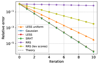
Refer to caption
Refer to caption
  (a) High-coherence synthetic matrix
Refer to caption
Refer to caption
(b) WESAD dataset
Refer to caption
Refer to caption
(c) CIFAR-10 dataset
Refer to caption
Refer to caption
(d) Musk dataset
Figure 4: Newton sketch for least squares regression. We use the sketch size m=4d𝑚4𝑑m=4d for all experiments. Results are averaged over 101010 trials.

E.4 Regularized least squares and effective dimension

On Figure 5, we report the error versus number of iterations of the Newton Sketch for regularized least squares regression. These results illustrate in particular our theoretical predictions: the convergence rate of Newton-LESS is upper bounded by deff/msubscript𝑑eff𝑚d_{\text{eff}}/m. In fact, Newton-LESS has the same convergence rate as the Newton Sketch with dense Gaussian embeddings.
Refer to caption
(a) High-coherence synthetic matrix
Refer to caption
(b) CIFAR-10 dataset
Refer to caption
(c) Musk dataset
Refer to caption
(d) WESAD dataset
Figure 5: Newton Sketch for regularized least squares regression. We use the sketch size m=4deff𝑚4subscript𝑑effm=4d_{\text{eff}} for all experiments. Results are averaged over 101010 trials.