Using a template engine as a computer algebra tool

Abstract

In research problems that involve the use of numerical methods for solving systems of ordinary differential equations (ODEs), it is often required to select the most efficient method for a particular problem. To solve a Cauchy problem for a system of ODEs, Runge–Kutta methods (explicit or implicit ones, with or without step-size control, etc.) are employed. In that case, it is required to search through many implementations of the numerical method and select coefficients or other parameters of its numerical scheme. This paper proposes a library and scripts for automated generation of routine functions in the Julia programming language for a set of numerical schemes of Runge–Kutta methods. For symbolic manipulations, we use a template substitution tool. The proposed approach to automated generation of program code allows us to use a single template for editing, instead of modifying each individual function to be compared. On the one hand, this provides universality in the implementation of a numerical scheme and, on the other hand, makes it possible to minimize the number of errors in the process of modifying the compared implementations of the numerical method. We consider Runge–Kutta methods without step-size control, embedded methods with step-size control, and Rosenbrock methods with step-size control. The program codes for the numerical schemes, which are generated automatically using the proposed library, are tested by numerical solution of several well-known problems.

I Introduction

Runge–Kutta methods are basic numerical methods for solving nonrigid systems of ordinary differential equations (ODEs). Numerical schemes of high orders (tenth and higher) with step-size control and dense output are well known. For many programming languages, there are libraries that implement the most efficient numerical schemes. The most well debugged codes were generated for Fortran 77 by Ernst Hairer and his colleagues; the codes were described in L_Hairer_1 ; L_Hairer_2 and are available online L_FortranCodes . These routines implement the methods DOPRI5 L_DORPRI1980 and DOPRI853 L_DORPRI1981 , which feature step-size control and dense output. The latter method also supports order switching between $8$ and $5$ for better performance when solving smooth problems.

The DOPRI5 and DOPRI853 subroutines are very well optimized and are included in many libraries and math packages, e.g., Matlab L_Matlab , Octave L_Octave , SciPy L_Scipy , SciLab L_Scilab , Boost C++ L_Boost , etc. However, for educational and research purposes, it is often required to search through a number of Runge–Kutta methods to select the optimal one for a particular problem kulyabov:2016:rk-stochastic ; kulyabov:2017:ceur:vol2064:runge-kutta ; kulyabov:2018:dccn:rk-stochastic . In addition, the efficiency of a particular numerical scheme also significantly depends on a problem to be solved.

To reliably compare different numerical schemes, we need a universal code that implements embedded methods for any set of coefficients. In this case, all implementations must be unified and differ only in their sets of coefficients.

To solve this problem, we propose a library for Julia L_JuliaLang_1 ; L_JuliaLang_2 ; L_JuliaLang_3 that consists of two parts: a computation part that implements algorithms of the Runge–Kutta type and a construction part that uses symbolic computations to generate specific versions of the Runge–Kutta algorithm and features automatic generation of function code from several ready-made templates. Initially, we considered implementing the construction part by using a universal computer algebra system, e.g., SymPy kulyabov:2020:rng-cas-sympy::en . However, in the process of implementation, it turned out that the main requirement for the computer algebra system was the support of template comparison. That is why we decided to use a lighter tool for symbolic manipulations. More specifically, instead of a full-featured computer algebra system, we use a template substitution tool. This approach, although somewhat exotic, is justified by a higher performance of the functions generated. For code generation, we use Python L_Python and Jinja2 template engine L_Jinja2 .

I.1 Paper structure

Section II briefly discusses embedded Runge–Kutta methods and step-size control strategy. Section III describes the developed library for Julia. Section IV presents the results of testing the functions generated automatically using the proposed library for the numerical solution of systems of ODEs. In particular, that section considers in detail the solution of the restricted three-body problem (problem of computing Arenstorf orbits).

II Runge–Kutta methods

In this paper, the Runge–Kutta methods are applied to a Cauchy problem formulated for a system of ODEs. The theory of Runge–Kutta methods is well known and described in detail in L_Hairer_1 ; L_Hairer_2 ; L_Butcher . Thus, in this section, we confine ourselves only to the basic formulas while briefly discussing the step-size control strategy implemented in our library.

II.1 Problem statement

Suppose that we have two smooth functions: $y^{\alpha}(t)\colon[t_{0},T]\to\mathbb{R}^{N}$ an unknown function and a known function $f^{\alpha}(t,y^{\beta}(t))\colon\mathbb{R}\times\mathbb{R}^{N}\to\mathbb{R}^{N}$, where $[t_{0},T]\in\mathbb{R}$ and $\alpha=1,\ldots,N$. Suppose also that the value of the function at the initial instant is known: $y^{\alpha}_{0}=y^{\alpha}(t_{0})$. Then, the Cauchy problem for a system of ODEs is formulated as follows:

$$\left\{\begin{aligned} &\dot{y}^{\alpha}(t)=f^{\alpha}(t,y^{\beta}(t)),\\ &y^{\alpha}(t_{0})=y^{\alpha}_{0},\;\alpha,\beta=1,\ldots,N.\\ \end{aligned}\right.$$ (1)

System (1) can be written component by component:

$$\left\{\begin{aligned} &\dot{y}^{1}(t)=f^{1}(t,y^{1}(t),\ldots,y^{N}(t)),\\ &\vdots\\ &\dot{y}^{N}(t)=f^{N}(t,y^{1}(t),\ldots,y^{N}(t)),\\ &y^{\alpha}(t_{0})=y^{\alpha}_{0}.\\ \end{aligned}\right.$$ (2)

On a segment $[t_{0},T]$, we define a grid from a set of points $t_{0}<t_{1}<t_{2}<\ldots<t_{k}<\ldots<t_{N}=T$ with a grid step $h_{k+1}=t_{k+1}-t_{k}$. Based on a certain rule called a numerical scheme, each point of the grid is associated with a certain value $y^{\alpha}_{k}$ that approximates (with desired accuracy) the solution of the system of ODEs at this point, i.e., $y^{\alpha}_{k}\approx y^{\alpha}(t_{k})$. To estimate approximation error, we use the norm $\|y^{\alpha}(t_{k})-y^{\alpha}_{k}\|$.

II.2 Embedded explicit Runge–Kutta methods

The error of the Runge–Kutta method can also be estimated in other way. The idea is that, in addition to the main solution $y^{\alpha}_{m}$ at a certain point, we also consider an auxiliary solution $\hat{y}^{\alpha}_{m}$ found by a Runge–Kutta method of an adjacent order. The difference between these solutions serves as an estimate for the local error of the lower-order method. This estimate facilitates the selection of a variable integration step. The methods that use the local error estimate are called embedded Runge–Kutta methods L_Hairer_1 . In this case, the method $y^{\alpha}_{m}$ is called main, while the method $\hat{y}^{\alpha}_{m}$ is called embedded.

An embedded explicit Runge–Kutta method for Cauchy problem (2) is given by the following formulas:

$$k^{1\alpha}=f^{\alpha}(t_{m},y^{\beta}_{m}),$$

$$\begin{multlined}k^{i\alpha}=f^{\alpha}\big{(}t_{m}+c^{i}h_{m},y^{\alpha}_{m}+h\sum^{i-1}_{j=1}a^{i}_{j}k^{j\beta}\big{)},\\ i=2,\ldots,s,\end{multlined}k^{i\alpha}=f^{\alpha}\big{(}t_{m}+c^{i}h_{m},y^{\alpha}_{m}+h\sum^{i-1}_{j=1}a^{i}_{j}k^{j\beta}\big{)},\\ i=2,\ldots,s,$$

$$\begin{multlined}y^{\alpha}_{m+1}=y^{\alpha}_{m}+h_{m}(b_{1}k^{1\alpha}+b_{2}k^{2\alpha}+{}\\ {}+\ldots+b_{s-1}k^{s-1,\alpha}+b_{s}k^{s\alpha}),\end{multlined}y^{\alpha}_{m+1}=y^{\alpha}_{m}+h_{m}(b_{1}k^{1\alpha}+b_{2}k^{2\alpha}+{}\\ {}+\ldots+b_{s-1}k^{s-1,\alpha}+b_{s}k^{s\alpha}),$$

$$\begin{multlined}\hat{y}^{\alpha}_{m+1}=y^{\alpha}_{m}+h_{m}(\hat{b}_{1}k^{1\alpha}+\hat{b}_{2}k^{2\alpha}+{}\\ {}+\ldots+\hat{b}_{s-1}k^{s-1,\alpha}+\hat{b}_{s}k^{s\alpha}),\end{multlined}\hat{y}^{\alpha}_{m+1}=y^{\alpha}_{m}+h_{m}(\hat{b}_{1}k^{1\alpha}+\hat{b}_{2}k^{2\alpha}+{}\\ {}+\ldots+\hat{b}_{s-1}k^{s-1,\alpha}+\hat{b}_{s}k^{s\alpha}),$$

where $N$ is the number of equations in the system of ODEs and $s$ is the number of stages in the numerical method. The Latin indices $i,j,l=1,\ldots,s$ are associated with the numerical scheme, the Greek indices $\alpha$ and $\beta$ are associated with the system of ODEs, while the subscript $m$ indicates the number of a step.

The orders of approximation by the grid functions $y^{\alpha}_{m}$ and $\hat{y}^{\alpha}_{m}$ are different, which makes it possible to compute approximation error at each step. Thus, to specify the order of the embedded method, we use the notation $p(\hat{p})$, where $p$ and $\hat{p}$ are the orders of the main and embedded Runge–Kutta methods, respectively.

The values $c^{i},a^{i}_{j},b_{j},\hat{b}_{j}$ completely define the numerical scheme and are called coefficients of the method; they are usually grouped in a Butcher table (named after John C. Butcher):

$$\begin{array}[]{c|cccccc}0&0&0&\ldots&0&0\\ c^{2}&a^{2}_{1}&0&\ldots&0&0\\ c^{3}&a^{3}_{1}&a^{3}_{2}&\ldots&0&0\\ \vdots&\vdots&\vdots&\ddots&\vdots&\vdots\\ c^{s-1}&a^{s-1}_{1}&a^{s-1}_{2}&\ldots&0&0\\ c^{s}&a^{s}_{1}&a^{s}_{2}&\ldots&a^{s}_{s-1}&0\\ \hline\cr&b_{1}&b_{2}&\ldots&b_{s-1}&b_{s}\\ &\hat{b}_{1}&\hat{b}_{2}&\ldots&\hat{b}_{s-1}&\hat{b}_{s}\end{array}$$

Finding the coefficients of the Runge–Kutta method for orders higher than fourth is a separate complex problem, which falls outside the scope of this paper and is described in detail in L_Hairer_1 . It should be noted, however, that it is common practice to impose the following additional conditions on the coefficients $c^{i}$ and $a^{i}_{j}$: $c^{i}=a^{i}_{1}+\ldots+a^{i}_{s}$.

To date, the coefficients for many embedded Runge–Kutta methods up to the tenth order of accuracy have been found. The most popular methods are those found by J.R. Dorman and P.J. Prince L_DORPRI1980 ; L_DORPRI1981 ; L_DORPRI1986 , E. Fehlberg fehlberg:1969:klassische-runge-kutta-funfter ; fehlberg:1970:klassische-runge-kutta-vierter , and J.R. Cash and A.H. Karp L_CashKarp1990 .

II.3 Step-size control strategy

There are various strategies for step-size (h) control depending on the local error. The choice of a particular strategy generally depends on a problem to be solved. Here, we employ the classical algorithm proposed by E. HairerL_Hairer_2 , which is based on ideas borrowed from control theory and works well for most nonrigid problems.

Suppose that $y^{\alpha}_{m}$ and $\hat{y}^{\alpha}_{m}$ are two numerical solutions of different approximation orders that are computed at the step $m$ of the algorithm. It is required that , where the desired scale $sc^{\alpha}$ is found by the formula

$$sc^{\alpha}=A_{tol}+\max(|y^{\alpha}_{m}|,|\hat{y}^{\alpha}_{m}|)R_{tol},$$

where $A_{tol}$ and $R_{tol}$ are the desired absolute and relative tolerances, respectively. The permissible error at the step $m$ is found as a root mean square:

$$E_{m}=\sqrt{\dfrac{1}{N}\sum\limits_{\alpha=1}^{N}{\left(\dfrac{y^{\alpha}_{m}-y^{\alpha}_{m}}{sc^{\alpha}}\right)^{2}}}.$$

A new step size is computed by the formula

$$h_{m+1}=h_{m}/\max\left(f_{\min},\min\left(f_{\max},E^{a}_{m}E^{-b}_{m-1}/f_{s}\right)\right),$$

where $E_{m-1}$ is the error found at the previous step. The factor $f_{s}$ (used to prevent a sharp increase in the step size) is generally $0.9$ or $0.8$. The exponents $a$ and $b$ are selected depending on a problem. In L_Hairer_2 , the following universal values were recommended: $a=0.7/p-0.75b$ and $b=0.4/p$, where $p$ is the order of approximation. The factors $f_{\min}$ and $f_{\max}$ set the step-size variation boundaries and also depend on a problem to be solved. In practice, the values $f_{\min}=0.1$ and $f_{\max}=5.0$ are generally selected.

In the case of $E_{m}<1$, the computed values $y^{\alpha}_{m}$ are considered satisfactory and the method goes to the next step. If $E_{m}>1$, then the results are considered unsatisfactory and the current step is repeated with a new value of $h_{m}$:

$$h_{m}\leftarrow h_{m}/\min\left(f_{\max},E^{a}_{m}/f_{s}\right).$$

At the next step $m+1$, as the initial value $y^{\alpha}_{m}$, we can use either directly $y^{\alpha}_{m}$ or the value yielded by the embedded method $\hat{y}^{\alpha}_{m}$.

III Description of the routine

III.1 Motivation to use code generation

Universal implementation of an embedded explicit Runge–Kutta method implies that, as parameters, the routine must receive arrays of coefficients from Butcher tables, which are then used in computations. Arrays seem to be a natural way to store these coefficients. However, $a^{i}_{j}$ is a lower-diagonal matrix and, when storing it as an $s\times s$ array, more than half of the memory allocated for the array is spent on storing zeros. The coefficients $c^{i}$, $b_{j}$, and $\hat{b}_{j}$ also often contain zeros, storing which is unreasonable.

That is why most codes that implement embedded explicit Runge–Kutta methods use a set of named constants (rather than arrays) to store the coefficients. Moreover, in most languages, scalar operations are faster than array operations.

In Julia, standard arrays are dynamic, which is why the overhead of storing a two-dimensional $s\times s$ array exceeds the overhead of storing $s\times s$ named constants.

To preserve the requirement for universality of the generated code while speeding up computations and reducing memory consumption, we decided to use automatic code generation based on one template for each individual method.

In addition to gaining in performance, automatic code generation allows us to add or modify all functions at once (rather than each function individually) by editing only one template. This also makes it possible to reduce the number of errors and generate different variants of functions for different purposes.

III.2 Description of the Runge–Kutta Generator

As a language for code generation, we chose Python because it supports various means for text manipulation. In addition, the standard Python library contains the Fraction data type, which allows us to set the Runge–Kutta coefficients as rational fractions and then convert them to real-valued form with desired order of accuracy.

In addition to Python, we also employ the Jinja2 template processing library L_Jinja2 . This template engine was originally designed for generating HTML pages. However, it has a very flexible syntax and can be used as a universal tool for generating text files of any kind, including source codes in any programming language. In combination with Jinja2, we use the numpy library L_Scipy to process arrays of coefficients.

The templates for generating functions are stored in the files rk_method.jl and erk_method.jl, which are Julia source codes with Jinja2 instructions. The template engine allows us to place the entire code generation logic in a template and input only the data associated with the method.

Information about numerical schemes is stored in a JSON file, where each method is a JSON object similar to the following one:

⬇

{"name": "Name (one word)",

"description": "Brief description",

"stage": ,

"order": ,

"extrapolation_order": ,

"a": [["0" , "0" , "0" ], ["1" , "0" ,

"0" ], ["1/4" , "1/4" , "0" ]],

"b": ["1/2" , "1/2" , "0" ],

"b_hat": ["1/6" , "1/6" , "2/3" ],

"c": ["0" , "1" , "1/2" ]}

The name of the JSON object is used as a name of a subsequently generated function. The arrays a, b, b_hat, and c can have either numeric or string type. If the method’s coefficients are set as rational fractions, then we can define them as "m/n". Further, they are converted to a Fraction object of the Python standard library; in the body of a function generated, they are represented as double-precision decimal fractions with $17$ significant digits.

The list of these objects is sequentially processed by the scripts erk_generator.py and rk_generator.py. By using the information about the methods, the scripts generate codes of several functions (in Julia) for each method.

These scripts generate functions for 16 embedded Runge–Kutta methods. Low-order methods are borrowed from L_Hairer_1 . For the methods of the fifth order and higher, we use the coefficients from L_DORPRI1980 ; L_DORPRI1981 ; L_DORPRI1986 and fehlberg:1969:klassische-runge-kutta-funfter ; fehlberg:1970:klassische-runge-kutta-vierter . The method from L_CashKarp1990 is implemented separately as it supports order switching and has a complex step-size control algorithm. To add user methods, it is required to create a JSON object (see above) and run the scripts to generate the corresponding functions for these methods.

III.3 Description of the functions generated

The developed library has a structure typical for Julia modules. The entire source code is stored in the src directory. The subdirectory src/generated contains files with automatically generated functions, which, in turn, are included in the main module file src/RungeKutta.jl by using the include directive. The code responsible for step-size control is stored in the file StepControl.jl and is common to all methods.

For each of the embedded Runge–Kutta methods, three functions are generated, two of which have the following form:

⬇

ERK(func, A_tol, R_tol, x_0, t_start, t_stop) -> (T, X)

ERK(func, A_tol, R_tol, x_0, t_start, t_stop, last) -> (t, x)

The functions have the same name and their lists of arguments differ only in the last argument. With Julia supporting multiple dispatch (function overloading), the compiler by itself determines which implementation needs to be called in each case.

In the functions described above,

• func::Function is the right-hand side of the system of ODEs $\dot{x}^{\alpha}(t)=f^{\alpha}(t,x^{\beta})$: func(t,x), where t::Float64 is time and x::VectorFloat64 is the value of the function $x(t)$; the argument $t$ must always be included in the function call, even if the system is autonomous and obviously does not depend on time;

• the arguments A_tol and R_tol are the absolute and relative accuracies of the methods, respectively; they must have the type Float64;

• x_0::Vector{Float64} is the initial value of the function $x^{\alpha}_{0}=x^{\alpha}(t_{0})$;

• t_start and t_stop are the start and end points of the integration interval, respectively; they have the type Float64;

• if the argument last::Bool is specified, then the end point of the integration interval $t_{n}$ and vector $x^{\alpha}_{n}\approx x^{\alpha}(t_{n})$ are returned; otherwise, the arrays T::Vector{Float64} and Matrix{Float64} are returned.

For the Runge–Kutta methods without step-size control, similar functions are generated with their only difference being the absence of the arguments A_tol and R_tol. Instead of them, the argument h, which specifies a step size used for computation, is passed.

To implement the step-size control algorithm, another function is generated:

⬇

ERK_info(func, A_tol, R_tol, x_0, t_start, t_stop) -> (accepted_t, accepted_h, rejected_t, rejected_h)

This function returns the following arrays:

• accepted_t: all grid points at which the computation error is considered satisfactory;

• accepted_h: all accepted step sizes;

• rejected_t: all grid points at which the computation error is considered unsatisfactory;

• rejected_h: all rejected step sizes;

• errors: values of the local error $E_{n}$.

All returned values have the type Vector{Float64}.

IV Testing the codes generated for the numerical schemes

To test the methods, we use three systems of differential equations considered in L_Hairer_2 . The first system is a system of van der Pol equations

$$\derivative[2]{x}{t}-\mu(1-x^{2})\derivative{x}{t}+x=0,$$

$$\left\{\begin{aligned} &\dot{x}_{1}(t)=x_{2}(t),\\ &\dot{x}_{2}(t)=\mu(1-x^{2}_{1}(t))x_{2}(t)-x_{1}(t),\end{aligned}\right.$$

with the initial values

$$\mu=1,\quad\mathbf{x}=(0,\sqrt{3})^{T},\quad 0\leqslant t\leqslant 12,$$

where the coefficient $\mu$ characterizes the nonlinearity and decay of oscillations.

The second system is a system of equations for a rigid body without external forces, i.e., a system of Euler’s equations for a rigid body:

$$\left\{\begin{aligned} &\dot{x}_{1}(t)=I_{1}x_{2}(t)x_{3}(t),\\ &\dot{x}_{2}(t)=I_{2}x_{1}(t)x_{3}(t),\\ &\dot{x}_{3}(t)=I_{3}x_{1}(t)x_{2}(t),\\ &I_{1}=-2,\;I_{2}=1.25,\;I_{3}=-0.5,\\ &\mathbf{x}=(0,1,1)^{T},\;t=[0,12].\end{aligned}\right.$$

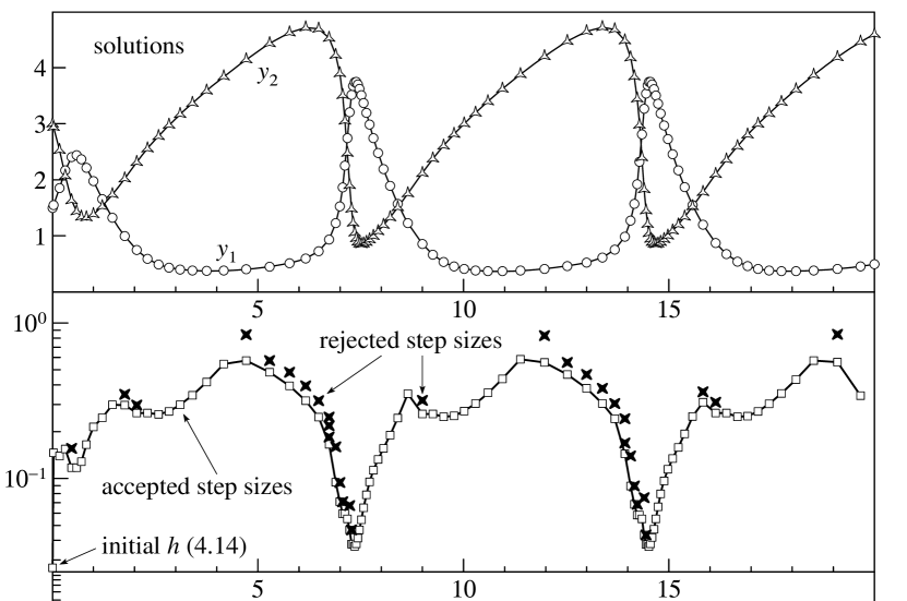
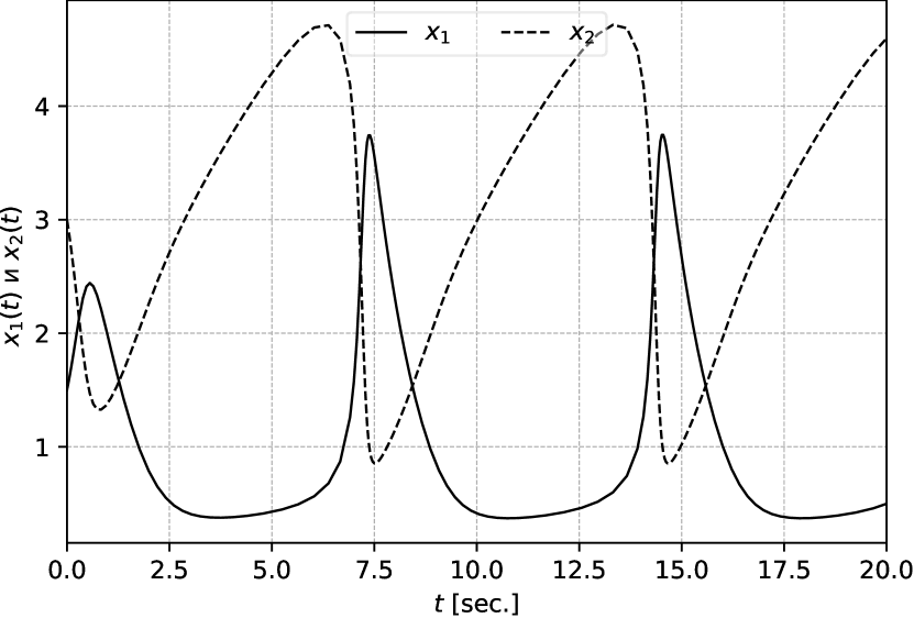
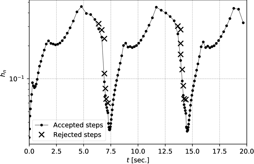
To test the step-size control algorithm, we apply the numerical scheme of the embedded Runge–Kutta method with $p=4$ and $\hat{p}=3$ to a system of Brusselator equations

$$\left\{\begin{aligned} &\dot{x}_{1}(t)=1+x^{2}_{1}x_{2}-4x_{1},\\ &\dot{x}_{2}(t)=3x_{1}-x^{2}_{1}x_{2}.\end{aligned}\right.$$ (3)

Under the initial conditions $x_{1}(0)=1.5$ and $x_{2}(0)=3$, the Brusselator equation is numerically integrated by the ERK43b method on a segment $0\leqslant t\leqslant 20$ with the absolute and relative tolerances $A_{tol}=R_{tol}=10^{-4}$. The corresponding graphs, which are identical to those from (L_Hairer_1, , p. 170, Fig. 4.1), are constructed. When comparing the results from L_Hairer_1 (see Fig. 1) and our results (see Figs. 2 and 3), it can be seen that our method performs almost identically to that from L_Hairer_1 ; however, our method selects step size more accurately.

Figure 1: Solution of system (3) with rejected and accepted steps  (L_Hairer_1, , p. 170, Fig. 4.1)

Figure 2: Solution of system (3)

Figure 3: Rejected and accepted steps for (3)

Another system of equations often used to test numerical schemes is a special case of the restricted three-body problem: the problem of computing Arenstorf orbits (named after an American physicist who computed a stable orbit of a small body between the Moon and the Earth).

The restricted three-body problem considers the motion of a small body in the gravitational fields of a medium body and large body (the Moon and the Earth). The mass of the small body is considered zero, while the masses of the medium and large bodies are $\mu_{1}$ and $\mu_{2}$, respectively. The orbits of the bodies are assumed to be on the same plane.

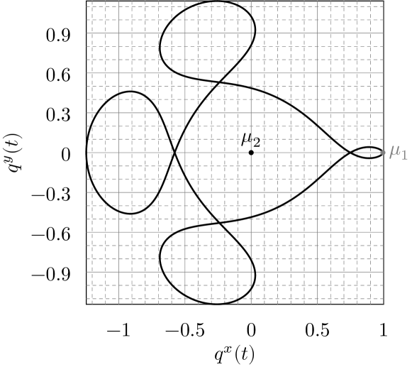
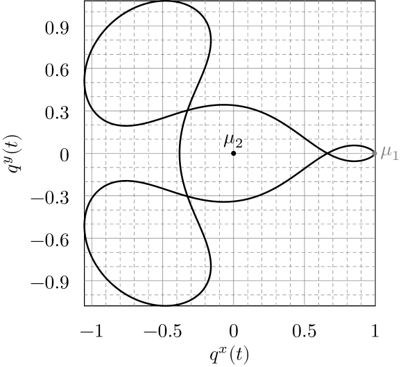
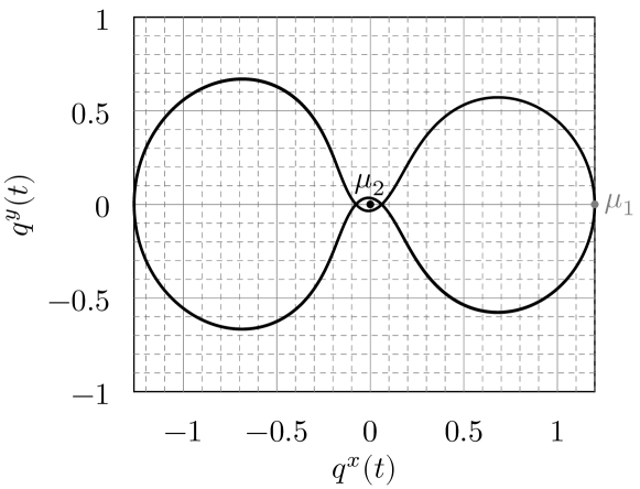
In the Arenstorf problem, different stable orbits can be obtained depending on initial values L_Hairer_1 . In dimensionless synodic coordinates, three groups of initial values, which provide three different orbits, have the following form:

$$\begin{gathered}p_{y}=-1.00758510637908238,\quad p_{x}=0.0,\\ q^{x}=0.994,\quad q^{y}=0.0;\end{gathered}$$ (4)

$$\begin{gathered}p_{y}=-1.03773262955733680,\quad p_{x}=0.0,\\ q^{x}=0.994,\quad q^{y}=0.0;\end{gathered}$$ (5)

$$\begin{gathered}p_{y}=0.15064248999999985,\quad p_{x}=0.0,\\ q^{x}=1.2,\quad q^{y}=0.0.\end{gathered}$$ (6)

Here, $p_{x}$ and $p_{y}$ are generalized momenta of the system, while $q^{x}$ and $q^{y}$ are generalized coordinates of the system.

It should be noted that the initial values are purposefully set with high accuracy because the small body very closely approaches the medium body and even a small computational error can lead to an incorrect physical interpretation (fall of the small body on the medium body). This makes the Arenstorf problem well suitable for testing implementations of numerical schemes.

The Hamilton function in synodic coordinates is written as follows:

$$H(p_{x},p_{y},q^{x},q^{y})=\frac{1}{2}(p_{x}^{2}+p_{y}^{2})+p_{x}q^{y}-p_{y}q^{x}-F(q^{x},q^{y}),$$

where

$$F(q^{x},q^{y})=\frac{\mu_{1}}{r_{1}}+\frac{\mu_{2}}{r_{2}},\quad\mu_{1}+\mu_{2}=1,$$

$$r_{1}=\sqrt{(q^{x}-\mu_{2})^{2}+(q^{y})^{2}},$$

$$r_{2}=\sqrt{(q^{x}+\mu_{1})^{2}+(q^{y})^{2}};$$

$$\partialderivative{F}{q^{x}}=-\frac{\mu_{1}(q^{x}-\mu_{2})}{r^{3}_{1}}-\frac{\mu_{2}(q^{x}+\mu_{1})}{r^{3}_{2}},$$

$$\partialderivative{F}{q^{y}}=-\frac{\mu_{1}q^{y}}{r^{3}_{1}}-\frac{\mu_{2}q^{y}}{r^{3}_{2}}.$$

The canonical equations to which the numerical scheme is applied have the following form:

$$\left\{\begin{aligned} &\dot{p}_{x}=+p_{y}+\partialderivative{F}{q^{x}},\dot{q}^{x}=p_{x}+q^{y},\\ &\dot{p}_{y}=-p_{x}+\partialderivative{F}{q^{y}},\dot{q}^{y}=p_{y}-q^{x}.\end{aligned}\right.$$

Numerical solution is carried out for $0\leqslant t\leqslant 17.065216560157962558$ with the absolute and relative tolerances $A_{tol}=10^{-17}$ and $R_{tol}=0$ and average mass $\mu_{1}=0.012277471$. As a result, we find Arenstorf orbits (see Figs. 6, 6, and 6) for initial values (4), (5), and (6), respectively.

Figure 4: Orbit for the first group of initial values (4)

Figure 5: Orbit for the second group of initial values (5)

Figure 6: Orbit for the third group of initial values (6)

To estimate the error, the system is solved numerically for a time interval equal to one period. At the end point of the interval, the small body must return to the start point, i.e., $(q^{x}(0),q^{y}(0))=(q^{x}(T),q^{y}(T))$, which is why the error $\|\mathbf{q}_{0}-\mathbf{q}_{n}\|$ corresponds to the global error of the method. The errors for the first group of initial values are shown in Table 1.

Table 1: Global errors of the numerical methods for one orbital revolution for the first group of initial values

Method	Error
DPRK546S	$1.84566\cdot 10^{-12}$
DPRK547S	$2.93634\cdot 10^{-12}$
DPRK658M	$4.22771\cdot 10^{-12}$
Fehlberg45	$7.42775\cdot 10^{-12}$
DOPRI5	$1.95463\cdot 10^{-13}$
DVERK65	$1.67304\cdot 10^{-12}$
Fehlberg78B	$5.45348\cdot 10^{-12}$
DOPRI8	$1.06343\cdot 10^{-11}$

V Conclusions

Thus, the main contribution of this work is as follows.

1. The language of the Jinja2 template engine has been used as a specialized symbolic computation system. As compared to a universal symbolic computation system, this approach has allowed us to make the software package simpler and more compact, as well as improve its portability.

2. A set of Python scripts has been created using the Jinja2 language; these scripts generate Julia codes that implement numerical schemes of Runge–Kutta methods without step-size control, embedded methods with step-size control, and Rosenbrock methods with step-size control (all the routines are available at https://bitbucket.org/mngev/rungekutta_generator).

3. The generated functions have been tested by solving several typical problems (in this paper, we have considered in detail the Arenstorf problem as it depends more heavily on the accuracy of a numerical scheme); the module for the Julia language is available at https://bitbucket.org/mngev/rangekutta-autogen.