The Effect of Continuum Elimination in Identifying Circumstellar Dust around Mira

Abstract

Asymptotic Giant Branch (AGB) stars are major contributors of cosmic dust to the universe. Typically, dust around AGB stars is investigated via radiative transfer (RT) modeling, or via simple deconstruction of observed spectra. However, methodologies applied vary. Using archival spectroscopic, photometric, and temporal data for the archetypal dusty star, Mira, we identify its circumstellar silicate dust grains. This is achieved by matching the positions and widths of observed spectral features with laboratory data. To do this comparison properly, it is necessary to account for the continuum emission. Here we investigate various ways in which a continuum is eliminated from observational spectra and how it affects the interpretation of spectral features. We find that while the precise continuum shapes and temperatures do not have a critical impact on the positions and shapes of dust spectral features, it is important to eliminate continua in a specific way. It is important to understand what contributes to the spectrum in order to remove the continuum in a way that allows comparison with laboratory spectra of candidate dust species. Our methodologies are applicable to optically thin systems, like that of Mira. Higher optical depths will require RT modeling, which cannot include many different potential astrominerals because there is a lack of complex refractive indices. Finally, we found that the classic silicate feature exhibited by Mira is not consistent with a real amorphous silicate alone but may be best explained with a small alumina contribution to match the observed FWHM of the $\sim 10\mu$m feature.

1 Introduction

Asymptotic Giant Branch (AGB) stars are major contributors of cosmic dust to the interstellar medium. Understanding the formation of cosmic dust ejected from these stars is essential to understanding the broader topics of evolution and composition of stellar and interstellar objects in our universe. We identify dust grains in space by matching the positions of observed spectral features with those seen in laboratory spectra. While radiative transfer modeling should allow us to build a spectrum that includes all contributions to the observed spectra, we are hampered by a paucity of appropriate laboratory data for such modeling. Typically, we need the complex refractive indices of candidate minerals in order to perform radiative transfer modeling. While there are many simple absorption or transmission spectra measurements for candidate minerals, very few minerals have corresponding complex refractive indices. This limits the application of radiative transfer modeling if we want to determine the detailed mineralogy of the dust.

In some cases (usually very optically thin scenarios), we can simply eliminate a continuum contribution to the observed spectrum to isolate any observed features and measure their basic spectral parameters (peak and barycentric positions, relative strength, FWHM) In this paper, we investigate several methods of continuum elimination to verify whether removing the continuum will affect the shape, strength, and position of the spectral features.

In § 2 we discuss relevant background including the theory behind continuum removal and previous studies that apply a variety of continuum elimination methods; in § 3 we give background information on Mira ($o$ Ceti) that is relevant to our study; in § 4 we describe the data and processing used to eliminate the continuum and measure the spectral features, while in § 5 the results of applying these methods are described. § 6 contains a discussion of the implications of our results.

2 background

2.1 Fitting the Continuum

To fit and remove the continuum from an observed spectrum, we need to consider what contributes to the photons we receive. If the dust shell is not very opaque (i.e., its optical depth is low), an observed spectrum can be represented by

$$F_{\rm tot}(\lambda)=F_{\star}(\lambda)+F_{\rm dust}(\lambda)$$ (1)

Some starlight is always obscured by the dust, which is why this equation is most applicable to optically thin situations. As optical depth increases, more starlight is removed and significant radiative transfer occurs, making this simple equation no longer accurate.

We can then break down the light emitted by the dust, $F_{\rm dust}$ (dustlight) as follows:

$$F_{\lambda}=F_{\star}+\sum_{i=1,j=1}^{n,m}C_{j}\times Q_{\lambda,j}\times B_{\lambda,i}(T_{i})$$ (2)

where each $B_{i}$ represents a single dust temperature blackbody (of which there are $n$ total), each $Q_{\lambda,j}$ represents the wavelength-dependent extinction efficiency for a single grain type as defined by its size, shape, composition, and crystal structure, and each $C_{j}$ represents the scale factor for a single grain type (of which there are $m$ total). This means that at each given wavelength the emission from the individual dust species is simply added to give the total emission at that wavelength.

It is possible to subtract the star’s contribution to the spectrum by using either an observed spectrum of a naked star of similar temperature (like e.g., Sloan et al., 2003A) or by using a stellar atmosphere model (from e.g., Allard, 2016). However, the precise details of the stellar spectrum, with all the molecular absorption features, especially those due to CO and SiO, are sensitive to the exact temperature and composition of the stellar atmosphere. The goal of this paper is not to accurately model the underlying star, but to assess the effects of the processes of deconstructing observed spectra of dusty stars on extracting data about the dust. Therefore, rather than applying a detailed model of the stellar atmosphere, we approximate the star as a blackbody with a temperature $T_{*}$. Subtracting the stellar flux $F_{\star}$ gives:

$$F_{dust}=\sum_{i=1,j=1}^{n,m}C_{j}\times Q_{j}\times B_{i}$$ (3)

In cases where the dust shell is optically thick, the starlight will be significantly extinguished and simply subtracting the star is difficult.

The spectrum is often simplified to:

$$F_{\lambda}=C\times Q_{\lambda}\times B_{\lambda}(T)$$ (4)

where $B_{\lambda}(T)$ is the Planck function for a blackbody of temperature $T$, $Q_{\lambda}$ is a composite value including contributions from all dust grains of various sizes, shapes, crystallinities, and compositions, and with a mean temperature $T$, and $C$ is a scale factor that depends on the number of dust particles, their geometric cross section, and the distance to the star. In the literature, this equation has been applied to the entire spectrum including the star; or it has been applied after subtraction of a stellar or blackbody spectrum (see § 2.2). Here we determine the sensitivity of the positions and shapes of spectral features to the simplification of the spectrum to Equations 1–4.

2.2 Previous studies with continuum elimination

Different methodologies have been used to eliminate the continua from stellar spectra to extract dust spectral features that follow the theory described in § 2.1. The usual techniques are continuum subtraction or division, but the choice of continuum shape also varies. The opacity (optical depth) of the dust shell should influence which method is used. As outlined in the previous section, if the circumstellar dust shell is optically thin, the spectrum of the star should be subtracted from the total flux to isolate the temperature-dependent spectrum of the dust. An optically thick dust shell will be dominated by the spectrum of the dust which will obscure the flux coming from the star. While previous work using continuum elimination has covered many different types of dust environments, here we focus on previous work on O-rich Asymptotic Giant Branch (AGB) stars.

Previous work which used continuum elimination methods include Sylvester et al. (1999), Dijkstra et al. (2005), and Speck et al. (2008) who all used the continuum division method. This is equivalent to applying Equation 4 to the whole spectrum. Sylvester et al. (1999) used data from the Infrared Space Observatory (ISO) Short- and Long-Wavelength Spectrometers (SWS and LWS, respectively) to examine a sample of seven oxygen-rich AGB stars with dense (optically thick) circumstellar dust shells. In these OH/IR stars, the dust completely obscures the stars at visible wavelengths. Mira was also presented for comparison. Their method used a “pseudo-continuum” spline-fit to approximate the general shape of this continuum. Division by a spline fitted continuum was also employed by Dijkstra et al. (2005) who examined 7-14-$\mu$m ISO spectra of a sample of 12 M-type evolved stars of varying mass-loss rates and therefore different optical depths. Both these papers use spline-fitting, which does not necessarily represent a real, physical cause for the continuum. Speck et al. (2008) also applied a continuum-division method, focused on IRAS 17485-2534, a highly obscured oxygen-rich AGB star. In this case, the continuum was modeled as a 400K blackbody rather than a spline fit. The match of the observed continuum to a single blackbody temperature would suggest that we are seeing an isothermal surface within the dust shell. This represents the depth at which the shell becomes optically thick. The lack of extra emission at longer wavelengths suggests that any outlying dust is low enough in density to have an insignificant contribution to the overall emission (c.f. Speck et al., 2009).

There are many examples of previous studies which used continuum-subtraction to extract dust spectral features. Volk & Kwok (1987) examined Infrared Astronomical Satellite (IRAS) Low-Resolution Spectrometer (LRS) 8-22$\mu$m spectra for a sample of 467 oxygen-rich AGB stars having a wide variety of optical depths. The continuum was fit with a power law of the form $F\propto$ $\lambda^{\beta}$ on either side of the 10-$\mu$m feature. The power-law fit is taken to represent the true continuum over the feature, and the strength of the feature is measured relative to the continuum. Little-Marenin & Little (1988) used a similar method to study the dust emission seen in IRAS LRS spectra of 79 MS, S, and SC stars. In this case, they fit a blackbody energy distribution to both sides of an emission feature and subtracted this continuum from the observed spectrum. Little-Marenin & Little (1990) applied a slightly different continuum to a larger sample of (291) Mira variables observed with IRAS LRS. In this study, they subtracted a 2500 K blackbody from each observed spectrum prior to classifying the shape and position of the $\sim$10$\mu$m spectral feature. Sloan & Price (1995) also used IRAS LRS spectra to investigate a sample of variable oxygen-rich AGB stars and the silicate emission at 10$\mu$m. They isolated dust emission by modeling the stellar continuum with a modified Planck function, fitting it to the spectra, and subtracting it. These studies all fit the star and subtracted it; they just approximated the star differently.

Following on from IRAS, researchers found new details in the spectra of cosmic dust from the ISO. While examining the 13-$\mu$m dust emission feature in ISO SWS spectra of optically-thin oxygen-rich circumstellar dust shells, Sloan et al. (2003A) eliminated the continua by fitting a naked (dust-free) oxygen-rich AGB star spectrum and subtracting it. The 131 stars in the sample are mostly AGB with some supergiants and objects transitioning between AGB and planetary nebula stages. Molster et al. (2002) used spectra from the ISO SWS and LWS to study a sample of 17 oxygen-rich circumstellar dust shells surrounding evolved stars, ranging from AGB stars to the planetary nebula phase and including some massive red supergiants and objects whose status are unclear. They used a spline fit to approximate the continuum, which they subtracted.

Speck et al. (2000) analyzed the ground-based (UKIRT) 8$-$13 $\mu$m spectra of 142 M-type stars, including 80 oxygen-rich AGB stars and 62 red supergiants. The dust features in the 10-$\mu$m region were examined using normalized, continuum-subtracted spectra. For each source, a 3000 K blackbody representing the stellar photosphere was normalized to the spectrum at 8.0-$\mu$m. This was then subtracted from the observed astronomical spectrum. It is also worth noting that varying the assumed 3000 K blackbody temperature by +/- 1000 K has very little effect on the size and shape of the derived continuum-subtracted dust features, but the precise positions were not measured. This is similar to the result found by DePew et al. (2006), where radiative transfer models showed that the stellar temperature does not have a major effect on positions and strengths of spectral features.

These different approaches have also been used to study various types of objects other than stars. Markwick-Kemper et al. (2007) looked at grain properties in the dust composition in a broad absorption line quasar observed with the Spitzer Space Telescope and used a power law to fit the continuum. The method included a continuum-divided spectrum, assuming the emission region is optically thin in the infrared. This is to yield the resulting opacity of the dust, and the temperature dependence has been eliminated by dividing the spectra by the continua. They also subtracted a spline-fit continuum of each spectrum to provide the same base line and ran models on the continuum-divided spectrum. Peeters et al. (2002) used ISO SWS spectra to fit continua for PAH bands using a sample of 57 sources including reflection nebulae, HII regions, YSOs, evolved stars, and galaxies. They used a variety of methods to extract the feature profiles including subtracting a local spine continuum, subtracting a polynomial of order 1, drawing a general continuum splined through chosen points, and drawing a continuum under features. It is worth noting that PAH spectral features are much narrower than the $\sim$10$\mu$m silicate feature, and thus, is less affected by difference in the choice of continuum.

Methods for eliminating the continuum have varied, and the effect of different methodologies has not been adequately explored. When working with a very optically thick system, the star is hidden visibly, and one may be able to divide by a blackbody. This blackbody represents the dust temperature in the circumstellar shell where the medium transitions from optically thin to optically thick. Division by the blackbody extracts the dust emission/absorption efficiencies ($Q_{\lambda}$) as given in Equation 4. When working with an optically thin system, simply subtracting a stellar continuum ($F_{\star}$) leaves a residual dust spectrum ($F_{\rm dust}$) that still depends on the dust temperature (see Equation 3). This temperature dependence has been largely neglected when measuring or classifying the residual dust spectral features. It should be noted that there are intermediate optical depths, where significant radiative transfer occurs such that the simplification to either Equation 1 (optically thin) or Equation 4 (optical thick) is not applicable. In these cases, it is necessary to apply full radiative transfer modelling.

Below, we explore the effect of applying Equations 1–4 as different pathways to isolating and measuring observed dust features using the optically thin star, Mira.

3 Mira as a case study

Mira has the distinction of being the first known variable star, having been discovered over 400 years ago. This pulsating AGB star has a period of 332 days, a V-band magnitude ranging 2-10.1, and spectral type M5–9IIIe. The temperatures corresponding to Mira’s spectral type range over 3420–2667 K (see the stellar spectral flux library by Pickles 1998). Mira itself exists as a binary system consisting of the AGB star (Mira A) and a compact accreting companion (Mira B), first seen optically in 1923 (Aitken). The classic $\sim$10$\mu$m silicate spectral feature was first observed in the late sixties in the infrared (IR) spectra of several M-type giants and red supergiants (RSGs) including Mira (Gillett et al., 1968).

This well-studied, archetypal, dusty star is used here to demonstrate that the analysis method affects the interpretation of dust spectral features and to find which method(s) of continuum elimination should be applied to the analysis of similar AGB stars.

Many dusty stars have been classified according to their mid-infrared (IR) spectra obtained by the IRAS LRS. Mira has been classified by Sloan & Price (1998) as infrared emission class SE8, indicating silicate and oxygen-rich dust composition with classic narrow silicate emission. Kraemer et al. (2002) classified Mira as infrared spectral class 2.SEc, representing strong silicate emission features with peaks at 10–12$\mu$m and 18–20$\mu$m. Sloan et al. (2003A) extended this work and classified Mira as IR spectral class 2.SE8, signifying a lack of a 13-$\mu$m feature. Speck et al. (2000) used UKIRT spectra to classify Mira’s dust features as silicate AGB A, indicating a “classic” narrow 9.7-$\mu$m silicate feature.

Mira displays the classic circumstellar $\sim$10 $\mu$m silicate dust emission feature seen in many dusty environments. Understanding the nature of the silicate dust is important to so many astrophysical environments (e.g., Videen & Kocifaj, 2002; Draine, 2003; Krishna-Swamy, 2005; Krugel, 2008; Mann et al., 2006; Casassus et al., 2001; Chiar et al., 2007; Hao et al., 2005) but interpreting this classic spectral feature is sensitive to how we extract it from our observations. In the next section we will investigate this sensitivity.

4 Measuring the Spectral Parameters

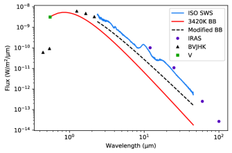
Figure 1: The spectral energy distribution for Mira together with the stellar blackbody spectrum (T = 3420 K) and the best fit modified blackbody. The black triangles are the flux values in the BVJHK bands; the purple dots are the flux values in the four IRAS photometry bands; the green square is the V-band flux for the same date as the ISO SWS observations; the blue line is the ISO SWS spectrum of Mira; the red line is a 3420 K blackbody fitted to the observed data at V-band; and the black dashed line is the best fit modified blackbody. The $x$-axis is wavelength in $\mu$m and the $y$-axis is flux density in Wm${}^{-2}\mu$m${}^{-}1$.

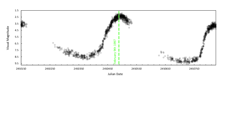
Figure 2: The V-band light curve for Mira over a $\sim$22-month period (2 full pulsation cycles) from AAVSO. The ISO SWS observation date is indicated by the dashed green line. The $x$-axis is Julian Date and the $y$-axis is visual magnitude.

Mira was observed using ISO SWS on February 9th, 1997. The fully processed post-pipeline spectral data were acquired from an online atlas associated with Sloan et al. (2003B). Detailed data reduction information is available from the atlas website accessed at https://users.physics.unc.edu/$\sim$gcsloan/library/swsatlas/aot1.html. We acquired the BVJHK photometric fluxes and the IRAS 12, 25, 60, and 100 $\mu$m photometry data from the SIMBAD astronomical database. In addition to the broad band magnitudes from SIMBAD, we also retrieved the V-band magnitude from the AAVSO database for the exact date of the ISO SWS observation. The resulting spectral energy distribution (SED) is shown in Figure 1.

The lightcurve from AAVSO shows that the observation date for the ISO SWS spectrum is close to that of the maximum brightness of Mira (Figure 2), allowing us to constrain the stellar temperature to the highest value for known spectral range of Mira, i.e., 3420 K. The V-band photometric data point for the observation date was used to normalize our stellar (3420 K) blackbody to the SED as shown in Figure 1.

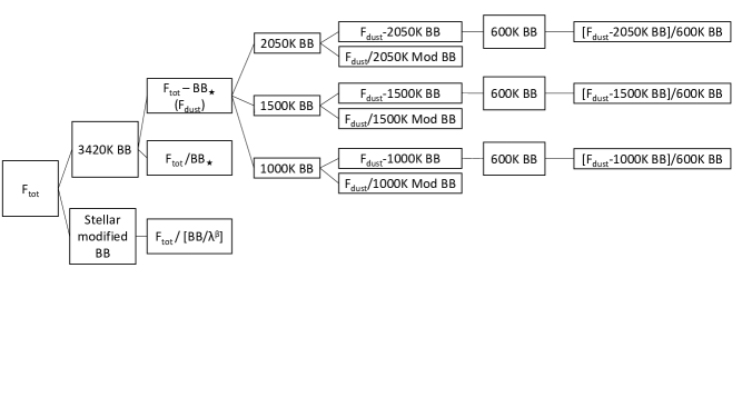
Figure 3: Continuum elimination pathways.

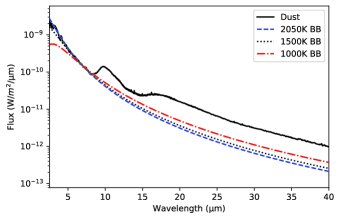
Figure 4: F_dust - the stellar-blackbody-subtracted, or total dust spectrum, for Mira together with the dust continuum blackbodies. The black line is F_dust; the dashed blue line is a 2050 K blackbody; the dotted black line is a 1500 K blackbody; and the dot-dash blue line is a 1000 K blackbody. The $x$-axis is the wavelength in $\mu$m and the y-axis is flux density in Wm${}^{-2}\mu$m${}^{-}1$.

To determine the sensitivity of spectral feature measurements to the choice of continuum elimination, we used six pathways, which fall into two categories: 1) Fit and subtract a stellar blackbody; or 2) fold the stellar contribution in equation 1 into the overall dust flux as in Equation 4.

If we subtract a stellar continuum, we must then subtract or divide a dust continuum. If we subtract a continuum, we must then fit another dust continuum and divide by it. If we divide by the continuum - we are left with some form of emission efficiency ($Q$-value). If we divide by the initial “stellar” continuum, we are assuming that Equation 4 applies, and we cannot make any more steps. We can only divide by a continuum once! The list of pathways, along with symbols/abbreviations is summarized in Table 1 and a flow diagram to show each pathway is given in Figure 3.

Table 1: Definitions of terms

Name/symbol	Definition
Ftot	the total flux coming from Mira and the surrounding circumstellar dust
Ftot/BB⋆	total flux received divided by stellar blackbody
Ftot/(BB/$\lambda^{\beta}$)	total flux received divided by a modified blackbody with emissivity index $\beta$
Fdust	total dust flux = total flux received with stellar blackbody subtracted
Fdust/(BB/$\lambda^{\beta}$)	total dust flux divided by a modified blackbody with emissivity index $\beta$
Fdust-BBdust1	total dust flux with a dust continuum subtracted
(Fdust-BBdust1)/BBdust2	total dust flux, with a dust continuum subtracted and then divided by a second dust blackbody continuum.

Following Equation 1, we can isolate the TOTAL emission from the dust by subtracting the stellar blackbody. The resulting dustlight spectrum ($F_{\rm dust}$) is shown in Figure 4. Once we subtract the star, the next step is to fit the dust continuum with either a regular or a modified blackbody where the modified version can be expressed as $BN=B\lambda^{\beta}$, and $\beta$ is the emissivity index for the dust. The dust continuum is then divided out to leave a continuum-eliminated spectrum (see e.g., Figure 5).

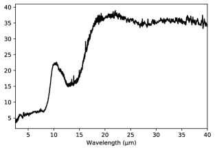
Figure 5: The ISO SWS spectrum of Mira divided by 3420 K stellar blackbody. $x$-axis is wavelength in $\mu$m and the $y$-axis is normalized flux.

We developed a program called MiraFitter which allows us to fit blackbodies (or modified blackbodies) to any spectrum. The original, flux calibrated ISO SWS data is $F_{\rm tot}=F_{\star}+F_{\rm dust}$, the total flux from both the star and the dust surrounding it. As described in Section 2.1, stars with optically thin dust will need the stellar flux subtracted in order for us to examine the dust. To fit a blackbody, MiraFitter uses a Planck curve for a given temperature; we can select the wavelength at which Planck curve is normalized to the observational spectral data. We can also apply a modification via an emissivity law (as described above, where $\beta$ is the emissivity index).

In addition to fitting blackbodies and/or modified blackbodies, MiraFitter analyzes the spectral features in each of the continuum-eliminated spectrum produced by following the 6 pathways shown in Figure 3 and Table 1 as well as in the original, total flux spectrum (F_tot). MiraFitter can find the peak position of the silicate emission features at $\sim$10 $\mu$m and $\sim$18 $\mu$m, calculate the barycentric positions of those features, and measure their full width half maxima (FWHM). While there is often an emphasis on the “peak position” for dust spectral features, both the peak and barycentric positions are important for discriminating between different potential astrominerals. The combination of the peak, barycenter, and FWHM gives a good measure of both the position and the shape of the spectral features. This will be discussed further below and in § 6.

To identify the peak positions around $\sim$10 $\mu$m and $\sim$18 $\mu$m in all the various continuum-eliminated spectra, MiraFitter determines the maximum flux in the ranges 9.5–10.5$\mu$m and 17.6–18.3$\mu$m and then the corresponding wavelength of each peak. These positions were examined visually to ensure that the peak measurement is not due to a noisy point in the observed spectrum. This methodology is applied to seven different versions of the same original spectrum (as listed in Table 1).

The barycentric position of a dust spectral feature is often not aligned with the peak position (see e.g. Speck et al., 2011). While barycenter is often used in terms of the center of mass of a system, in spectroscopic terms, the barycenter of a spectral feature is the wavelength at which the energy within the feature is split exactly in half. Therefore, we need to calculate the area under the curve of the spectral feature and split that area in half to find the centroid or barycenter. The barycentric positions of the $\sim$10$\mu$m and $\sim$18$\mu$m features as well as the FWHM for the $\sim$10$\mu$m are listed in Table 2. The $\sim$18 $\mu$m peaks are not consistently defined, and FWHM values are not reported. It should be noted that many previous studies of dust features simply fit the continuum either side of the silicate features at 10 and 18$\mu$m (e.g., Volk & Kwok, 1987; Little-Marenin & Little, 1988), which does yield a clearly defined 18$\mu$m feature. But the application of this method will shift the position of the observed feature and make comparison to laboratory data difficult. This will be discussed further in § 6.

As described in Section 2.1, Equation 4 has been applied to analyzing the whole spectrum including both dust and starlight. In this case, the version of the spectrum that is considered continuum eliminated is F_tot/BB_⋆, i.e., the total flux divided by the blackbody spectrum of the star. This is best applied when the system is optically thick and there is little direct starlight to remove (e.g., Sylvester et al., 1999; Speck et al., 2009). More examples of work that has used this version of continuum elimination are given in Section 2.2.

The F_tot/BB_⋆ spectrum is shown in Figure 5, while the F_tot/(BB/$\lambda^{\beta}$) spectrum (divided by modified blackbody) is shown in Figure 6.

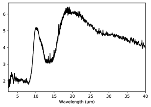
Figure 6: The ISO SWS spectrum of Mira divided by a modified blackbody. $x$-axis is wavelength in $\mu$m and the $y$-axis is normalized flux.

When the system is optically thin enough that the total spectrum ($F_{\rm tot}$) is dominated by direct starlight, we must subtract the stellar blackbody to isolate the emission from dust ($F_{\rm dust}=F_{\rm tot}$ – $F_{\star}$, see Equation 1). There is always some uncertainty in the stellar temperature, especially for variable stars. In many studies, AGB stars have been assumed to be 3000 K for simplicity. Mira itself has a range of temperatures from 2667 K to 3420 K. To determine whether the precise temperature of a stellar continuum affects the peak position of the spectral dust feature, we varied the stellar blackbody temperature. We found that temperatures above 2493 K and above could be used before the peak positions around $\sim$10 $\mu$m and $\sim$18 $\mu$m are affected. The TOTAL dust spectrum (i.e., the stellar-blackbody-subtracted spectrum) F_dust is plotted in Figure 4.

Applying a blackbody modified by an emissivity law (BB/$\lambda^{\beta}$) as the continuum may be appropriate, depending on the precise nature of the dust. The emissivity index, $\beta$, depends on the size, structure, composition, and temperature of the dust grains as well as the optical depth of the dust shell (e.g. Demyk et al., 2017, and references therein). While in reality $\beta$ should have a value in the range 1-2 to have a physical meaning (Koike et al., 1987; Mennella et al., 1998), laboratory experiments have shown that it is possible to have emissivity indices outside this range (Koike et al., 1980, where amorphous carbon has a $\beta\approx 0.8$). Moreover, a negative $\beta$ value can be used to mimic a continuum that is the sum of several blackbodies of differing temperatures. Figure 7 demonstrates that using a negative $\beta$ value emulates the summing of several blackbodies of different temperatures into a single spectrum. In this case, the value of $\beta$ reflects the range of temperatures and the total amount of dust at each temperature.

For fitting a modified blackbody to our Mira SED, the value of $\beta$ was varied until the best fit (by eye) was achieved. This is established using a visual tool within MiraFitter that displays both the spectrum being fitting and the fitting modified blackbody as well as a plot of the resultant divided spectrum. The presence of both the silicate features and the numerous molecular absorption feature makes a chi-squared minimization difficult to apply, but the divided spectrum should be flattened (on average, ignoring the dust and molecular features). This fitting process yielded $\beta$ = -0.5. This best-fitting modified blackbody is shown with the SED in Figure 1. A range of $\beta$ values were tested to determine at what values the peak positions were affected. The $\sim$10 $\mu$m peak is unchanged for -0.79 $\leq\beta\leq$ -0.03, and the $\sim$18 $\mu$m peak is unchanged for -1.99 $\leq\beta\leq$ 0.0. It is notable that the beta value is always negative, indicative of a range of dust temperatures combining to give the continuum (see Figure 7.) In fact, that we can simply sum a series of blackbodies to replicate a negative $\beta$ value is consistent with Equation 3 where the dust spectrum is a sum of blackbodies with emission efficiencies applied.

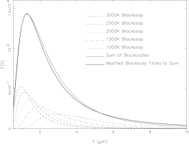
Figure 7: A demonstration of the effect of summing blackbodies on the continuum-fitting process. $x$-axis is wavelength in $\mu$m; $y$-axis is flux density in arbitrary units.

Once we have removed the stellar contribution from the spectrum (i.e., generated $F_{\rm dust}$), we then fit another blackbody to account for the temperature-dependent dust continuum. There are several ways to conceptualize the dust “continuum”. It could be the blackbody ($B_{\lambda}(T)$) from Equation 4, in which case, division by said blackbody would yield the emission efficiency factor $Q_{\lambda}$ for a composite dust species including contributions from all dust grains of various sizes and assuming a single mean temperature. Alternatively, the continuum could be due to a collection of dust grains that contribute to the overall continuum but do not display diagnostic spectral features (e.g., metallic iron). In this case, the continuum would be one of the $C_{j}\times Q_{j}\times B_{i}$ components in Equation 3, and thus subtracting the continuum to isolate the dust with spectral features is appropriate. Note that in this case we are still left with another $C_{j}\times Q_{j}\times B_{i}$ component and this residual spectrum is still temperature dependent.

To test the effect of different dust continua, we created blackbodies of 1000 K, 1500 K, and 2050 K for removal. The fits of these continuum blackbodies to the total dust spectrum is shown in Figure 4. The conventional (most common) choice for the dust continuum temperature is based on the identification of the $\sim$10 $\mu$m feature as amorphous or glassy silicate. Approximately 1000 K is the typical silicate glass transition temperature (see Speck et al., 2011). Above the glass transition, the silicate grains will either form directly as crystalline material or an amorphous solid will begin crystallizing. The other temperatures we chose coincide with (1) the condensation temperature for olivine and pyroxene; $\sim$1500 K; and (2) best fit to the total dust spectrum, F_dust without any theoretical considerations about dust stability; 2050 K. While 2050 K is above the stability temperature for any silicates, it is not an unfeasible temperature for the first solids to form (e.g., high temperature oxides, aluminates or titanates; McSween, 1989; Ebel, 2006). Furthermore, there is a molecular layer in the atmosphere of Mira with a temperature of 1500–2100 K (Perrin, 2004). In addition, this 2050 K blackbody was the best fit for the total dust spectrum and thus serves to test (a) the sensitivity to getting the best fitting continuum rather than using a physically expected value and (b) the effect of temperature on the resulting spectral feature parameters.

Assuming that most of the dust is silicate and that the dust emission can be modeled according to Equation 4, we need to divide by the dust-continuum temperature to extract the temperature-independent parameters ($Q$-values) of the dust spectral features.

As with the measurement of the spectral feature parameters in the total dust spectrum (F_dust), we wanted to test for the effect of varying the star temperature used to generate $F_{\rm dust}$ prior to dividing out the dust continuum: i.e., we want to know whether there are downstream effects on the spectral feature parameters that depend on early steps in the pathway to continuum elimination. After dividing out the dust continuum, the peak position of silicate spectral features at $\sim$10 $\mu$m and $\sim$18 $\mu$m remain unchanged for all stellar temperatures greater than 2493 K, well within the known temperature of Mira for the observation date.

In addition, F_dust/(BB/$\lambda^{\beta}$) uses emissivity after subtracting the star. A new blackbody is constructed using dust temperatures of 1000, 1500 and 2050 K, as described above, normalized at 7  $\mu$m. Each blackbody was modified by an emissivity law; the emissivity index, $\beta$, was varied until the best fit (by eye, using the methodology described above) was achieved. This gave $\beta$ = -0.9, which works for all temperatures above 411 K. The resulting spectra are shown in Figure 8 (top row). A range of $\beta$ values was tested to determine its effect on spectral feature parameters. The peak positions remain unchanged for -0.74 $\leq$ $\beta$ $\leq$ -1.96. The position and shape of the spectral features is not very sensitive to the temperature or value of emissivity index.

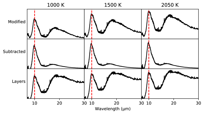
Figure 8: The effect of different dust continuum elimination. Each column shows the temperature labeled at the top for the blackbody used for continuum removal. The top row uses a modified blackbody and is the total dust spectrum divided by the blackbody dust continuum for that column, i.e., F_dust/(BB/$\lambda^{\beta}$); the middle row shows the total dust spectrum with the dust continuum blackbody subtracted, i.e. F_dust-BB_dust1; and the bottom row is the same as the middle row, but with a 600 K blackbody divided out. i.e., (F_dust-BB_dust1)/BB_dust2.

It is possible that the blackbody fitted to the star-subtracted spectrum (F_dust) represents a different dust component than silicate (for example, metallic iron or some form of high-temperature oxide). In that case, it is necessary to subtract the dust blackbody to isolate the emission from silicate. Then we need to fit a new blackbody to account for the temperature of the silicate dust. Figure 8 (middle row) shows this F_dust-BB_dust1, with the dust blackbody curve subtracted from the original F_dust. The spectral features at $\sim$10 $\mu$m and $\sim$18 $\mu$m in the F_dust-BB_dust1 (dust continuum subtracted spectrum) have peak positions that remain the same for a dust temperature range of 1000–3200 K.

The final step is to determine the intrinsic spectral parameters for the silicate features in this 2-dust component scenario. Since this leaves a residual spectrum that is still temperature-dependent, we then fit a second blackbody curve for a dust layer at 600 K, which was divided out to give us the temperature-independent $Q$-values, i.e., (F_dust-BB_dust1)/BB_dust2, shown in Figure 8 (bottom row). The $\sim$10 $\mu$m peak is unchanged for the second dust layer having temperatures ranging 203$-$663 K, and the $\sim$18 $\mu$m peak is unchanged for temperatures above 225 K.

5 Measurement Results

The results of the spectral feature measurements described in § 4 are summarized in Table 2. We have tested the effect on spectral parameters of using different temperatures and emissivity indices and found that the measurements are not very sensitive to either temperature or emissivity index. However, Table 2 shows that the precise pathway to continuum elimination can have a large impact on the peak position, barycenter, and FWHM of the spectral features.

For the $\sim$10 $\mu$m feature, the peak position is consistent for all pathways to continuum eliminations that start with subtraction of the stellar blackbody, whereas the $\sim$18 $\mu$m is more sensitive to the next steps in the continuum elimination. For the pathways to continuum elimination that do not start with subtracting the star, even the $\sim$10 $\mu$m feature varies. The barycentric positions for both the $\sim$10 $\mu$m and $\sim$18 $\mu$m features shows similar trends with the $\sim$18 $\mu$m peak position, showing that division by a continuum has a major effect on how we measure the position of the silicate features. The implications of these results are discussed in § 6.

Table 2: Spectral Feature Measurements

	Peak position ($\mu$m)		Barycenter		FWHM
	$\sim 10\mu$m	$\sim 18\mu$m	$\sim 10\mu$m	$\sim 18\mu$m	($\mu$m)
Ftot	9.83	17.64	10.15	17.75	2.18
Ftot/BB⋆	10.37	18.20	10.49	19.06	2.87
Ftot/(BB/$\lambda^{\beta}$)	10.12	18.20	10.44	18.97	2.77
Fdust	9.83	17.64	10.16	17.74	2.05
1000 K Fdust/(BB/$\lambda^{\beta}$)	9.83	18.20	10.36	18.83	2.36
1500 K Fdust/(BB/$\lambda^{\beta}$)	9.83	18.20	10.39	18.86	2.47
2050 K Fdust/(BB/$\lambda^{\beta}$)	9.83	18.20	10.40	18.88	2.54
1000 K Fdust-BBdust1	9.83	17.64	10.20	18.27	2.36
1500 K Fdust-BBdust1	9.83	17.64	10.19	18.20	2.34
2050 K Fdust-BBdust1	9.83	17.64	10.19	18.16	2.34
1000 K (Fdust-BBdust1)/BBdust2	9.83	18.20	10.37	18.93	2.70
1500 K (Fdust-BBdust1)/BBdust2	9.83	18.20	10.37	18.93	2.76
2050 K (Fdust-BBdust1)/BBdust2	9.83	18.20	10.37	18.93	2.76

6 Discussion

Figure 9: Laboratory absorbance spectra for samples from (Speck et al., 2011). In all cases the $x$-axis is the wavelength in $\mu$m and the $y$-axis is absorbance. The dotted line indicates the barycentric positions for the $\sim$10 $\mu$m and $\sim$18 $\mu$m features. The wavelengths of the peak positions are listed in Table 3.

We investigated the positions and shapes of the $\sim$10 $\mu$m and $\sim$18 $\mu$m spectral features using different analysis methods.

We identify dust components in circumstellar spectra by comparing with laboratory data. The precise composition and structure of a silicate will affect the parameters of the $\sim$10 $\mu$m and $\sim$18 $\mu$m of spectral features. Comparing the laboratory data parameters from Speck et al. (2011), shown in Table 3 and Figures 9 and 10, and the peak positions and barycenters extracted from the Mira spectrum (shown in Table 2), we can see that incorrect continuum elimination will lead to incorrect attributions of minerals to circumstellar features.

Table 3: Spectral Parameters of Glasses from Speck et al. (2011) (all units are $\mu$m)

Sample	Peak		Barycenter		FWHM
Name	$\sim$10$\mu$m	$\sim$18$\mu$m	$\sim$10$\mu$m	$\sim$18$\mu$m	$\sim$10$\mu$m
Gehlenite	10.3		10.8		2.86
Akermanite	10.3		10.6		2.46
Forsterite	10.2		10.4		2.43
Diopside	10.1	19.2	10.2	19.4	2.46
Basalt	10.0		9.9		2.41
Enstatite	9.9	17.6	9.9	18.5	2.58
Cosmic silicate	9.8	18.3	9.7	18.7	3.15
Obsidian	9.0		9.1		2.14
Herasil (SiO2)	9.0		8.9		1.34

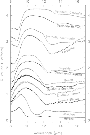
Figure 10: Calculated Q-values (absorption efficiency factors) for samples from Speck et al. (2011). These Q-value spectra are stacked to demonstrate the shift in wavelength of the peak of the $\sim$10 $\mu$m with composition.

For instance, the $\sim$10 $\mu$m feature peaks at 9.8-9.9$\mu$m for both Enstatite and “Cosmic Silicate” but their $\sim$18 $\mu$m features peak at 17.6$\mu$m and 18.3$\mu$m, respectively. This means that F_tot and F_dust are consistent with Enstatite, but F_dust/(BB/$\lambda^{-\beta}$) and (F_dust-BB_dust1)/BB_dust2 are consistent with “Cosmic Silicate”. Meanwhile the continuum-elimination pathways that do not subtract the star would suggest a match to Forsterite or Gehlenite.

When we focus on the barycentric position of the features (rather than peak position), we see similar trends with the $\sim$18 $\mu$m peak position. The barycentric position of both silicate features is shifted whenever a continuum division is involved in the process of continuum elimination.

Comparing the measured barycenters to those for laboratory samples listed in Table 3, we see that the $\sim$10 $\mu$m feature matches diopside (CaMgSiO₄) most closely when there is no continuum division in the elimination pathway but is closer to forsterite for continuum elimination that uses a divided continuum. Unfortunately, we do not have a measurement of the $\sim$18 $\mu$m feature for this forsterite glass, but the diopside $\sim$18 $\mu$m feature occurs at a significantly longer wavelength than that observed for Mira in any version of the continuum elimination.

The comparison of both the peak position AND the barycentric position of the dust spectral features is critical to identifying their mineral carriers. Simply measuring the peak position will not suffice.

In addition to the peak and barycentric positions of the observed spectral features, we also measured the FWHM of the $\sim$10 $\mu$m feature. It is clear from the list in Table 2 that the FWHM is quite sensitive to the choice of continuum elimination pathway. Unlike the peak position and barycenter, the FWHM is sensitive to the choice of continuum temperature, making the parameter difficult to use to identify potential mineral carriers.

We need to compare like with like, i.e., ensure that what we take from laboratory data is equivalent to observational data to which we compare. This is discussed extensively in Speck (2013). Figure 10 shows the $Q_{\lambda}$ values for a range of silicate glass compositions, while Figure 9 shows the wavelength dependent absorbance for the silicate glasses for which Speck et al. (2011) measured the $\sim$18 $\mu$m feature. Absorbance is closer to an optical depth than a $Q$-value.

Looking back at § 2.1, we can see for a fairly optically thin dust shell like that of Mira, we should subtract the stellar continuum (see Eqn 2). This leaves us with a temperature- dependent dust spectrum as given in Eqn 4. To extract the emission/absorption efficiency, we must divide the observed spectrum by the blackbody temperature of the dust. Without dividing by the dust continuum AFTER subtraction of the star, we should not compare to the $Q$-values.

Many of the studies of silicate features in circumstellar dusts, like those mentioned in § 2.2, simply subtract the stellar continuum and do not completely eliminate the dust continuum. Thus, those spectra cannot be used to infer the mineralogy of the dust.

If we follow any of the continuum elimination pathways that use both stellar continuum subtraction and dust continuum division, we find that for Mira the peak positions of the silicate features are consistently at 9.83 and 18.20$\mu$m, while the barycenters occur at 10.4 and 18.9$\mu$m (with a little more variability than the peak position). The peak position is consistent with “Cosmic Silicate” while the barycentric position is not. This may suggest the need for a non-silicate component (e.g., alumina; Speck et al., 2000), even in this archetypal strong silicate feature.

It is clear from this study that care must be taken when deconstructing observational spectroscopic data. While radiative transfer modeling may be able to provide a more accurate representation of the temperatures of dust involved in the emission of photons at each wavelength, RT modeling is hampered by a lack of applicable laboratory data. Most radiative transfer modeling uses synthetic complex refractive indices (or dielectric constants) such as Draine & Lee (1984); Ossenkopf, Henning, & Mathis (1992). However, these optical constants are not based on real mineral samples and cannot allow us to extract mineralogical information from observed spectra (see Speck et al., 2015, and references therein). Moreover, there are problems with many of the published refractive indices that are based on real mineral samples (Speck et al., 2011). Consequently, it is difficult to use RT modeling when the goal is to extract the detailed dust mineralogy.

Here we have shown that for low optical depth systems, we MUST subtract a stellar contribution from the observed total spectrum (see Equation 1) - but the precise $T_{\star}$ value is not critical. Then we must divide by a dust continuum in order to get a spectrum equivalent to the emission efficiency $Q_{\lambda}$ (i.e., applying Equation 4). In this case we generate F_dust/(BB/$\lambda^{\beta}$) and include the step of subtracting a featureless continuum due to e.g., metallic iron will not change the relevant parameters of the silicate features (although the overall feature-to-continuum ratio may be affected). Failure to subtract a stellar continuum OR divide by a dust continuum will lead to incorrect feature parameters and thus to misidentified astrominerals. As optical depth increases, the application of this simplified deconstruction method becomes problematic and RT modeling becomes necessary. However, at very high optical depth, there are several examples of systems where the continuum can be fitted by a single blackbody (e.g., Speck et al., 2008, 2009). In this case we are observing an isothermal layer in the dust shell outside of which the dust is optically thin. We usually apply Equation 4 to determine the $Q_{\lambda}$ values for the absorbing dust in the optically thin outer layers, but further study should be undertaken to determine what affect this has, versus treating the isothermal layer as the central “stellar” source.

7 Conclusions

We find that for optically thin dust shells, it is possible to deconstruct their spectra to extract detailed mineralogical information. However, the precise pathway by which continua are eliminated has significant effects on the residual dust spectrum and may lead to misidentification of dust species in space. For moderate to high optical depth systems, we cannot apply this simple deconvolution and must apply RT modeling. Unfortunately, RT modeling is hampered by a paucity of complex refractive indices for detailed mineralogical studies. To continue investigating dust in space we need to (a) acquire optical constants (complex refractive indices) of more real mineral samples; and (b) revisit the many studies of optically thin systems that have classified the silicate features with a new eye to understanding the detailed mineralogy.

Finally, our study suggests that the archetypal/classic silicate feature exhibited by Mira is not consistent with a real amorphous silicate alone, but may be best explained with a small alumina contribution to match the observed FWHM of the $\sim 10\mu$m feature.

Data Availability

The data underlying this article are available in publicly. The datasets were derived from sources in the public domain: (1) ISO SWS spectroscopic observational data from https://users.physics.unc.edu/$\sim$gcsloan/library/swsatlas/aot1.html; (2) all photometric data points were retrieved from SIMBAD (http://simbad.u-strasbg.fr/simbad/); and (3) lightcurve data from the AAVSO (https://www.aavso.org/).

References

- Aitken (1923) Aitken R. G., 1923, PASP, 35, 323
- Allard (2016) Allard, F., 2016, in SF2A-2016: Proceedings of the Annual meeting of the French Society of Astronomy and Astrophysics. Eds.: C. Reylé, J. Richard, L. Cambrésy, M. Deleuil, E. Pécontal, L. Tresse and I. Vauglin, pp.223-227.
- Casassus et al. (2001) Casassus, S., Roche, P. F., Aitken, D. K., Smith, C. H. 2001, MNRAS, 320, 424.
- Chiar et al. (2007) Chiar, J. E., Ennico, K., Pendleton, Y. J., et al. 2007, ApJ, 666, L73.
- Demyk et al. (2017) Demyk, K., Meny, C., Lu, X.-H., et al. A&A, 600, 123.
- DePew et al. (2006) DePew K., Speck A., Dijkstra C., 2006, ApJ, 640, 971
- Dijkstra et al. (2005) Dijkstra C., Speck A. K., Reid R. B., Abraham P., 2005, ApJ, 633, L133
- Draine & Lee (1984) Draine, B. T., Lee, H. M. 1984, ApJ, 285, 89.
- Draine (2003) Draine, B.T., 2003, ARA&A, 41, 241
- Ebel (2006) Ebel, D. 2006, in Meteorites and the Early Solar System II, D. S. Lauretta and H. Y. McSween Jr. (eds.), University of Arizona Press, Tucson, 943 pp., p.253-277.
- Gillett et al. (1968) Gillett, F. C., Low, F. J., Stein, W. A. 1968, ApJ, 154, 677.
- Hao et al. (2005) Hao, Lei, Spoon, H. W. W., Sloan, G. C., et al. 2005, ApJ, 625, L75.
- Koike et al. (1980) Koike, C., Hasegaqwa, H., Manab e, S., 1980, Ap&SS, 67, 495.
- Koike et al. (1987) Koike, C., Hasegaqwa, H., Hattori, T., 1987, Ap&SS, 134, 95.
- Kraemer et al. (2002) Kraemer K. E., Sloan G. C., Price S. D., Walker H. J., 2002, ApJS, 140, 389
- Krishna-Swamy (2005) Krishna Swarmy, K. S., 2005 “Dust in the Universe: Similarities And Differences”, World Scientific Series in Astronomy and Astrophysics, Vol. 7. Singapore: World Scientific Publishing, ISBN 981-256-293-1, 2005, XI + 252 pp.
- Krugel (2008) Krugel, E. 2008, “An Introduction to the Physics of Interstellar Dust” Taylor & Francis Group, LLC, New York, p387.
- Little-Marenin & Little (1988) Little-Marenin I. R., Little S. J., 1988, ApJ, 333, 305
- Little-Marenin & Little (1990) Little-Marenin I. R., Little S. J., 1990, AJ, 99, 1173.
- Mann et al. (2006) Mann, Ingrid, Köhler, Melanie, Kimura, Hiroshi, Cechowski, Andrzej, Minato, Tetsunori, 2006, A&ARev, 13, 159.
- Markwick-Kemper et al. (2007) Markwick-Kemper F., Gallagher S. C., Hines D. C., Bouwman J., 2007, ApJ, 668, L107
- McSween (1989) McSween, H. Y., 1989, American Scientist, 77, 146.
- Mennella et al. (1998) Mennella, V., Brucato, J. R., Colangeli, L., Palumbo, P., Rotundi, A., Bussoletti, E., 1998, ApJ, 496, 1058.
- Molster et al. (2002) Molster F. J., Waters L. B. F. M., Tielens A. G. G. M., Barlow M. J., 2002, A&A, 382, 184
- Ossenkopf, Henning, & Mathis (1992) Ossenkopf, V., Henning, Th., & Mathis, J. S. 1992, A&A, 261, 567.
- Peeters et al. (2002) Peeters E. et al., 2002, A&A, 390, 1089
- Perrin (2004) Perrin, G., Ridgway, S. T., Mennesson, B., et al. 2004, A&A, 426, 279.
- Pickles (1998) Pickles A. J. 1998, PASP, 110, 863
- Sloan et al. (2003A) Sloan G. C., Kraemer K. E., Goebel J. H., Price S. D., 2003A, ApJ, 594, 483
- Sloan et al. (2003B) Sloan G. C., Kraemer K. E., Price S. D., Shipman R. F., 2003B, ApJS, 147, 379
- Sloan & Price (1995) Sloan G. C., Price S. D., 1995, ApJ, 451, 758
- Sloan & Price (1998) Sloan G. C., Price S. D., 1998, ApJS, 119, 141
- Speck et al. (2000) Speck A. K., Barlow M. J., Sylvester, R. J., Hofmeister, A. M., 2000, A&A, 146, 437
- Speck et al. (2008) Speck A. K., Whittington A. G., Tartar J. B., 2008, ApJ, 687, L91
- Speck et al. (2009) Speck, A. K., Corman, A. B., Wakeman, K., Wheeler, C.H., Thompson, G., 2009, ApJ, 691, 1202.
- Speck et al. (2011) Speck A. K., Whittington A. G., Hofmeister, A. M., 2011, ApJ, 740, 93
- Speck (2013) Speck, A., 2013, in Proceedings of The Life Cycle of Dust in the Universe: Observations, Theory, and Laboratory Experiments, eds. A. Anderson, M. Baes, H. Gomez, C. Kemper, and D. Watson, Taipei, Taiwan, LCDU2013.
- Speck et al. (2015) Speck A. K., Pitman, K. M., Hofmeister, A. M., 2015, ApJ, 809, 65.
- Sylvester et al. (1999) Sylvester R. J. et al., 1999, A&A, 352, 587
- Videen & Kocifaj (2002) Videen, G., Kocifaj, M., 2002 Optics of Cosmic Dust: proceedings of a NATO Advanced Research Workshop NATO Science Series. Dordrecht/Boston/London: Kluwer Academic Publishers, 2002.
- Volk & Kwok (1987) Volk K., Kwok S., 1987, ApJ, 315, 654
- Yang et al. (2004) Yang X. H., Chen P., He J., 2004, A&A, 414, 1049
- Yang et al. (2007) Yang X. H., Chen P., Wang J., He J., 2007, A&A, 463, 663