PC-MLP: Model-based Reinforcement Learning
with Policy Cover Guided Exploration

Abstract

Model-based Reinforcement Learning (RL) is a popular learning paradigm due to its potential sample efficiency compared to model-free RL. However, existing empirical model-based RL approaches lack the ability to explore. This work studies a computationally and statistically efficient model-based algorithm for both Kernelized Nonlinear Regulators (KNR) and linear Markov Decision Processes (MDPs). For both models, our algorithm guarantees polynomial sample complexity and only uses access to a planning oracle. Experimentally, we first demonstrate the flexibility and efficacy of our algorithm on a set of exploration challenging control tasks where existing empirical model-based RL approaches completely fail. We then show that our approach retains excellent performance even in common dense reward control benchmarks that do not require heavy exploration. Finally, we demonstrate that our method can also perform reward-free exploration efficiently. Our code can be found at https://github.com/yudasong/PCMLP.

1 Introduction

Model-based Reinforcement Learning (MBRL) has played a central role in Reinforcement Learning for decades and has achieved great empirical performance on tasks such as robotics (Deisenroth & Rasmussen, 2011; Levine & Abbeel, 2014) and video games (Kaiser et al., 2019). However, most existing empirical model-based RL approaches lack the ability to perform strategic exploration. Thus they usually can not guarantee any global performance.

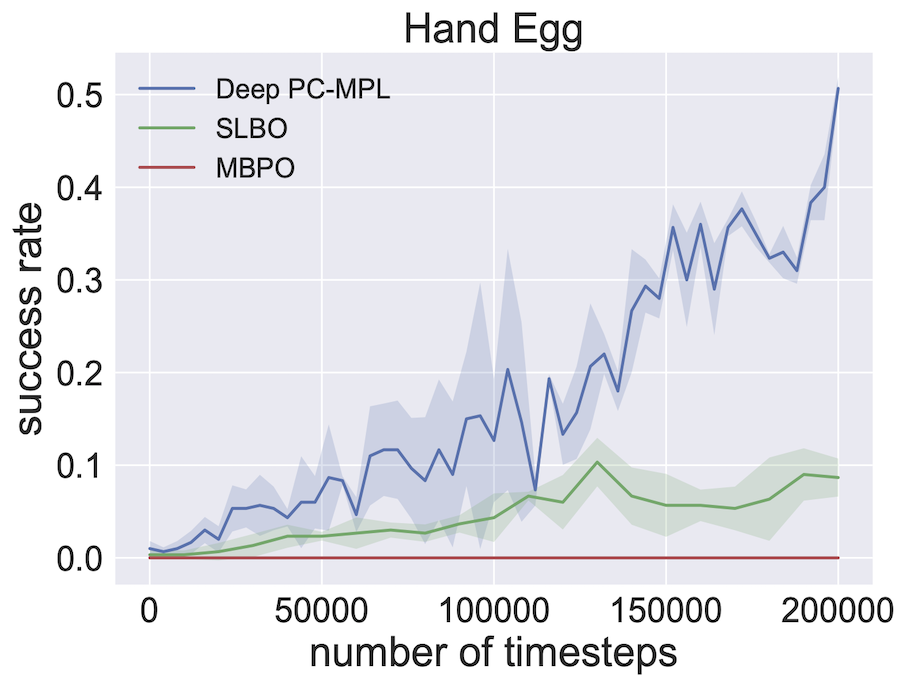
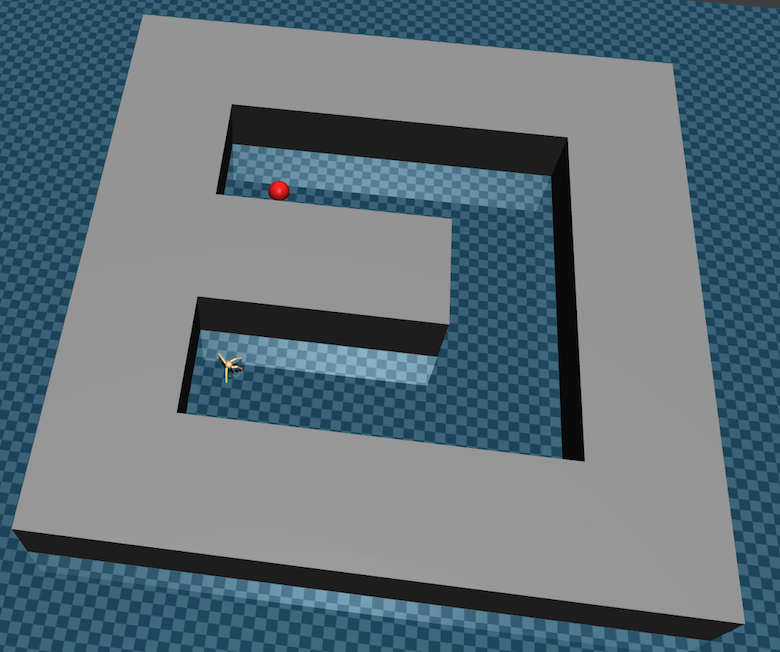
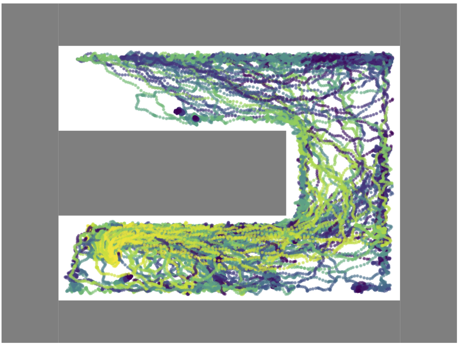
Figure 1: Example of the exploration ability of PC-MLP in the HandEgg and AntMaze experiments. The environments involve complex dynamics and sparse/no reward. Top Left: the HandEgg environment. Top Right: PC-MLP can explore strategically and thus learns much faster than other MBRL (SLBO and MBPO) baselines which rely on random exploration. Bottom Left: the AntMaze environment where we perform reward-free exploration. Bottom Right: coverage map of 5 policies in the policy cover (policy 10, 20, 30, 40 and 50). Thus PC-MLP can efficiently explore the maze without an explicit reward signal.

In this work, we consider learning to control a nonlinear dynamical system. Specifically, we focus on systems that can be modeled via Reproducing Kernel Hilbert Spaces (RKHS). Following (Kakade et al., 2020), we name such models Kernelized Nonlinear Regulators (KNRs). Such model has been extensively used in the robotics community in the last two decades due to its flexibility to capture popular models such as linear dynamics (LQRs), piece-wise hybrid linear system, nonlinear models that can be modeled by higher-order polynomials, and systems that can be captured by Gaussian Processes (GPs) (e.g., (Ko et al., 2007; Deisenroth & Rasmussen, 2011; Bansal et al., 2017; Fisac et al., 2018; Umlauft et al., 2018; Mania et al., 2020)). The fact that KNRs have been widely used in real-world robotics and control problems proves that KNR is capable to model real-world dynamics. Thus it motivates the development of algorithms that have global performance guarantees and are also provably sample and computation efficient for KNRs.

(Kakade et al., 2020) initiated an information theoretical analysis for KNRs and provided an algorithm (LC3) that achieves near-optimal regret. However, the proposed LC3 algorithm relies on an optimistic planning oracle (see Sec. 3 for the detailed definition of an optimistic planning oracle) which is unfortunately not computationally efficient. Thus, LC3 algorithm cannot be easily implemented using off-shelf computational tools developed from the planning and control community (e.g., highly efficient planning oracles). While its regret analysis is novel and tight, the computation inefficiency dramatically limits the practical usage of LC3. In this work, we develop a Model-based algorithm named PC-MLP, standing for Model Learning and Planning with Policy Cover for Exploration, that is provably sample efficient (i.e., polynomial in all relevant parameters), and is also planning-oracle efficient, i.e., it only requires access to a classic planning oracle rather than an optimistic planning oracle. Thus PC-MLP allows one to leverage existing off-shelf efficient planning oracles from the motion planning and control community, which provide excellent flexibility when deploying the algorithm to real-world control problems.

From RL side, several new linear MDP models (Yang & Wang, 2019; Jin et al., 2019; Modi et al., 2020; Zhou et al., 2020) recently have gained a lot of interest in the theoretical RL community, although unlikely KNRs, these linear MDP models haven’t been demonstrated to be applicable in real world problems. While our focus in this work is on KNRs due to their proven applicability to real-world robotics problems, we nevertheless also analyze our algorithm directly on linear MDPs. Note that linear MDPs are different from KNRs as linear MDPs cannot capture simple linear dynamical systems such as LQR.

Our contributions in this work are twofold. First, theoretically, we provide a single algorithm framework PC-MLP that is provably sample efficient, and computation-wise is planning-oracle efficient (i.e., no more optimistic planning) in both KNRs and Linear MDPs (Yang & Wang, 2019), simultaneously. Our algorithm is modular and simple. It maintains a policy cover (i.e., an ensemble that contains all previous learned policies) and learns a model from the traces of the policies in the cover. Policy cover avoids catastrophic forgetting issues when fitting the model (i.e., during model fitting, the latest model overfits to the current policies’ traces). The algorithm also uses a simple reward bonus scheme that is motivated by classic linear bandit algorithms (Dani et al., 2008) and also recent RL algorithms that work beyond tabular settings (Agarwal et al., 2020a). Unlike count-based reward bonus, our bonus works provably on continuous state and actions space. Empirically, we develop a practical version of PC-MLP—Deep PC-MLP, which uses deep neural network for model fitting, and random features (either Random fourier features (Rahimi & Recht, 2008) or random network based features (Burda et al., 2019)) for reward bonus design. We evaluate Deep PC-MLP extensively on common continuous control benchmarks including both sparse/no reward environments (e.g., sparse reward hand manipulation and high-dimensional reward-free maze shown in Fig. 1) and dense reward environments. Our algorithm achieves excellent performance in both exploration challenging control tasks and reward-free exploration tasks, and the classic dense reward control tasks.

This paper is structured as follows: in section 2 we provide additional related works. Section 3 introduces the KNRs and linear MDPs settings, notations, and basic assumptions. In section 4 we describe our algorithm framework, PC-MLP, while in section 5 we provide the main results on the sample complexity of PC-MLP in both linear MDPs and in KNRs. We then describe a practical implementation of PC-MLP using deep neural networks in section 6. Sections 7 includes a comprehensive empirical evaluation of the practical implementation.

2 Related Works

Below we discuss additional related works. On the theoretical side of KNRs, (Mania et al., 2020) studied KNRs from a system identification perspective. Their approach relies on a reachability assumption and a Lipschitz assumption on state-action features. Our work does not require any of the two assumptions. The high-level intuition is that if there is a subspace that is not reachable, it does not matter in terms of policy optimization as no policy can reach that subspace to collect rewards. When specializing in LQR, there are a lot of prior works studying sample complexity of learning in LQRs (Abbasi-Yadkori & Szepesvári, 2011; Dean et al., 2018; Mania et al., 2019; Cohen et al., 2019; Simchowitz & Foster, 2020). Optimal planning oracle in LQR exists and has a closed-form solution of the optimal control policy.

On the RL side, in both theory and in practice, model-based approaches are often considered to be sample efficient (Deisenroth & Rasmussen, 2011; Levine & Abbeel, 2014; Chua et al., 2018; Sun et al., 2018; Kurutach et al., 2018; Nagabandi et al., 2018; Luo et al., 2018; Ross & Bagnell, 2012; Sun et al., 2019; Osband & Van Roy, 2014; Ayoub et al., 2020; Lu & Van Roy, 2019). Many existing empirical MBRL algorithms lack the ability to perform exploration and thus cannot automatically adapt to exploration challenging tasks. Existing theoretical works either do not apply to KNRs directly or rely on optimistic planning oracles or a Thompson sampling approach which only guarantees a regret bound in the Bayesian setting.

3 PRELIMINARIES

We consider episodic finite horizon MDPs $\mathcal{M}=\{{\mathcal{S}},\mathcal{A},H,r,P^{\star},s_{0}\}$ where $s_{0}$ is a fixed initial state, ${\mathcal{S}}$ and $\mathcal{A}$ are continuous state and action space, $H\in\mathbb{N}^{+}$ is the horizon, $r:{\mathcal{S}}\times\mathcal{A}\mapsto[0,1]$ is the reward function, and $P^{\star}:{\mathcal{S}}\times\mathcal{A}\mapsto\Delta({\mathcal{S}})$ is the Markovian transition. In our learning setting, we assume reward $r$ is known but transition $P^{\star}$ is unknown. The learner is equipped with a policy class $\Pi\subset{\mathcal{S}}\mapsto\Delta(\mathcal{A})$, and the goal is to search for an optimal policy $\pi^{\star}\in\Pi$, such that $\pi^{\star}\in\mathop{\mathrm{argmax}}_{\pi\in\Pi}J(\pi;r,P^{\star})$, where $J(\pi;r,P):=\mathbb{E}\left[\sum_{h=0}^{H-1}r(s_{h},a_{h})|a_{h}\sim\pi(\cdot|s_{h}),s_{h+1}\sim P(\cdot|s_{h},a_{h})\right]$ is the expected total reward of $\pi$ under a transition $P\in{\mathcal{S}}\times\mathcal{A}\mapsto\Delta({\mathcal{S}})$ and reward $r:{\mathcal{S}}\times\mathcal{A}\mapsto[0,1]$. In additional to policy class $\Pi$, a model-based learner is also equipped with a model class $\mathcal{P}\subset{\mathcal{S}}\times\mathcal{A}\mapsto\Delta({\mathcal{S}})$. Throughout the paper, we assume realizability in model class:

Assumption 1 (Model Realizability).

We assume $\mathcal{P}$ is rich enough such that $P^{\star}\in\mathcal{P}$.

We require the sample complexity of our learning algorithm to depend only on the complexity measures of the model class $\mathcal{P}$.

The goal is to find an $\epsilon$-near optimal policy from $\Pi$, i.e., a policy $\hat{\pi}$ such that $J(\hat{\pi};r,P^{\star})\geq\max_{\pi\in\Pi}J(\pi;r,P^{\star})-\epsilon$, with high probability, using number of samples scaling polynomially with respect to all relevant parameters including the complexity of the model class $\mathcal{P}$. With the above setup, we discuss two specific examples.

Kernelized Nonlinear Regulators

For a KNR, we denote the transition as $s^{\prime}=W^{\star}\phi(s,a)+\epsilon$ where ${\mathcal{S}}\subset\mathbb{R}^{d_{s}}$, $\epsilon\sim\mathcal{N}(0,\sigma^{2}I)$, $\|W^{\star}\|_{F}\leq F\in\mathbb{R}^{+}$, and $\phi:{\mathcal{S}}\times\mathcal{A}\mapsto\mathbb{R}^{d}$ is potentially a nonlinear mapping. In other words, $P^{\star}(\cdot|s,a)=\mathcal{N}(W^{\star}\phi(s,a),\sigma^{2}I)$. Here $\phi$ is known, $\sigma$ is known, but $W^{\star}$ is unknown to the learner. When $\phi$ corresponds to some kernel feature mapping, $W^{\star}\phi(s,a)$ falls into the corresponding Reproducing Kernel Hilbert Space (RKHS). In this case, the model class $\mathcal{P}$ consists of transitions parameterized by $W$ with $\|W\|_{F}\leq F$. We can denote $\mathcal{W}=\{W:\|W\|_{F}\leq F\}$. It is clear that $W^{\star}\in\mathcal{W}$. Prior work LC3 relies on an optimistic planning oracle, i.e., $\max_{W\in\text{Ball}}\max_{\pi\in\Pi}J(\pi;r,W)$ with $\text{Ball}\subset\mathcal{W}$.

Linear MDPs

We consider a specific linear MDP model $P^{\star}(s^{\prime}|s,a)=\langle\mu^{\star}(s^{\prime}),\phi(s,a)\rangle,\forall s,a,s^{\prime}$ with $\phi:{\mathcal{S}}\times\mathcal{A}\mapsto\mathbb{R}^{d}$, where we assume $\mu^{\star}\in\Upsilon\subset{\mathcal{S}}\mapsto\mathbb{R}^{d}$. Here $\mu^{\star}$ is unknown but $\phi$ is known. Recently (Agarwal et al., 2020b) show that such linear model has a latent representation interpretation. For this model we assume $\Upsilon$ is finite and $\mu^{\star}\in\Upsilon$. For norm bound, we assume $\|\mu\cdot\nu\|_{2}\leq\sqrt{d}$ for any $\nu\in\mathbb{R}^{|{\mathcal{S}}|}$ with that $\|\nu\|_{\infty}\leq 1$. The statistical complexity of the model class is the log of the cardinality of $\Upsilon$, i.e., $\ln\left\lvert\Upsilon\right\rvert$. This model does not directly capture the linear MDP proposed by (Jin et al., 2019), but captures the version from (Yang & Wang, 2019) due to its finite degree of freedom in the linear model’s parameterization. The algorithm from (Yang & Wang, 2019) also relies on optimistic planning with value iteration to be the specific planning oracle.

Note that two models, linear MDPs and KNRs, are different: one does not generalize the other. While linear MDP generalizes the usual tabular MDPs, the Gaussian noise makes KNRs are unable to generalize tabular MDPs directly. However KNRs generalizes polynomial dynamical systems (i.e., linear system $s^{\prime}=As+Ba+\epsilon$) while linear MDPs cannot.

Despite the differences in two models, we present a single model-based algorithmic framework that takes $\mathcal{P}$ and $\Pi$ as inputs, and outputs an $\epsilon$ near-optimal policy $\pi$ in sample complexity scaling polynomially with respect to $H,1/\epsilon,d$ and the complexity of $\mathcal{P}$, with a polynomial number of calls to a planning oracle $\text{OP}(\Pi,r,P)$.

Assumption 2 (Planning Oracle).

Given reward $r$, transition $P$, and $\Pi$, we assume access to a planning oracle: $\text{OP}(\Pi,r,P):=\mathop{\mathrm{argmax}}_{\pi\in\Pi}J(\pi;r,P)$.

We treat OP as a black-box planning oracle and we do not place any restrictions on the form of the oracle. It could be a trajectory optimization based motion planner and controller (Ratliff et al., 2009; Todorov & Li, 2005; Sun et al., 2016) or it could be an asymptotically optimal sampling-based planner (Williams et al., 2017a; Karaman & Frazzoli, 2011). Note that $\text{OP}(\Pi,r,P)$ is a computation oracle which does not use any real-world samples.

The algorithm framework simultaneously applies to both KNR and Linear MDPs, with $\mathcal{P}=\left\{P(\cdot|s,a):\mathcal{N}(W\phi(s,a),\sigma^{2}I),\forall s,a\>|\>\|W\|_{F}\leq F\right\}$ and $\mathcal{P}=\left\{P(\cdot|s,a):\mu\phi(s,a),\forall s,a\>|\>\mu\in\Upsilon\right\}$ as model class inputs, respectively,

Additional Notations

We denote $d^{\pi}_{h}\in\Delta({\mathcal{S}}\times\mathcal{A})$ as the state-action distribution induced by policy $\pi$ at time step $h$, and $d^{\pi}=\sum_{h=0}^{H-1}d^{\pi}_{h}/H$ as the average state-action distribution from $\pi$.

4 Algorithm Framework

0:  MDP $\mathcal{M}$, inputs $(N,K,\lambda,M,\mathcal{P},c)$

1:  Initialize $\pi_{1}$

2:  Set policy-cover $\bm{\pi}_{1}=\{\pi_{1}\}$

3:  for $n=1\to N$ do

4:     Draw $K$ samples $\{s_{i},a_{i}\}\sim d_{\pi_{n}}$

5:     Set $\widehat{\Sigma}_{\pi_{n}}=\sum_{i=1}^{K}\phi(s_{i},a_{i})\phi(s_{i},a_{i})^{\top}/K$

6:     Set covariance matrix $\widehat{\Sigma}_{n}=\sum_{i=1}^{n}\Sigma_{\pi_{i}}+\lambda I$

7:     Model Learning (MLE) with data from policy-cover $\bm{\pi}_{n}$ and denote $\widehat{P}_{n}$ as an approximate optimizer of the following optimization program:

$$\max_{P\in\mathcal{P}}\sum_{i=1}^{M}\ln P(s_{i}^{\prime}|s_{i},a_{i})$$ (1)

where $\{s_{i},a_{i}\}\sim d_{\bm{\pi}_{n}},s^{\prime}\sim P^{\star}_{s_{i},a_{i}},\forall i\in[M]$

8:     Set reward bonus $\widehat{b}_{n}$ as in Eq. 2

9:     Plan $\pi_{n+1}=\text{OP}\left(\Pi,r+\widehat{b}_{n},\widehat{P}_{n},\right)$

10:     Update policy-cover: $\bm{\pi}_{n+1}=\bm{\pi}_{n}\oplus\{\pi_{n+1}\}$

11:  end for

Algorithm 1 The PC-MLP Framework

In this section, we introduce our algorithmic framework. Alg. 1 summarizes the algorithm PC-MLP standing for Model Learning and Planning using Policy Cover for Exploration.

In high-level, the algorithm maintains a policy cover $\bm{\pi}_{n}=\{\pi_{1},\dots,\pi_{n}\}$ that contains all previously learned policies. In each episode, the model learning procedure is a maximum likelihood estimation on training data collected by $\bm{\pi}_{n}$. Sampling from $\bm{\pi}_{n}$ can be implemented by first sampling $i\in[1,\dots,n]$ uniformly random, and then sample $(s,a)$ from $d^{\pi_{i}}$. The model $\widehat{P}_{n}$ trained this way (via the classic Maximum Likelihood Estimation) can predict well under state-action pairs covered by $\bm{\pi}_{n}$. This forces the learned model to achieve good prediction performance under the state-action pairs that are covered by the current policy cover $\bm{\pi}_{n}$.

For state-action pairs that do not well covered by $\bm{\pi}_{n}$, we design reward bonus. Specifically, we form the (unnormalized and regularized) empirical covariance matrix of the policy cover $\bm{\pi}_{n}$, i.e., $\widehat{\Sigma}_{n}=\sum_{i=1}^{n}\Sigma_{\pi_{i}}+\lambda I$. Intuitively, any state-action pair $(s,a)$, whose feature $\phi(s,a)$ falls into the subspace corresponding to the eigenvectors of $\widehat{\Sigma}_{n}$ with small eigenvalues, is considered as novel. Concretely, we design reward bonus as:

$$\widehat{b}_{n}(s,a)=\min\left\{2c\sqrt{\phi(s,a)^{\top}\widehat{\Sigma}_{n}^{-1}\phi(s,a)},H\right\}$$ (2)

with $c$ being a parameter. Note we truncate it at $H$ just because we know that the total reward is always upper bounded by $H$. To gain an intuition of the reward bonus, we can think about the tabular MDP as a special case here. To model tabular MDPs, one can design $\phi(s,a)\in\mathbb{R}^{|{\mathcal{S}}|\mathcal{A}|}$ as a one-hot vector that encodes state-action pair $(s,a)$. In this case, $\widehat{\Sigma}_{n}$ is a diagonal matrix and a diagonal entry approximates the probability of $\bm{\pi}_{n}$ visiting the corresponding state-action pair.

With reward bonus to encourage further exploration at novel state-action pairs, we invoke the planning oracle $\textrm{OP}(\Pi,r+\widehat{b}_{n},\widehat{P}_{n})$ to search for the best policy from $\Pi$ that optimizes the combination $r+\widehat{b}_{n}$ under the empirical model $\widehat{P}_{n}$. The intuition here is that the optimal policy $\pi_{n+1}$ returned by the planning oracle can visit novel state-action pairs due to the reward bonus. Thus the new policy cover $\bm{\pi}_{n+1}$ expands the coverage of $\bm{\pi}_{n}$, which leads to exploration.

Such iterative framework—iteratively fitting model and collecting new data using the optimal policy of the learned model, is widely used in practical model-based approaches (e.g., (Ross & Bagnell, 2012; Kaiser et al., 2019)), and our framework simply designs additional reward bonus for the planning oracle. There are prior works that leverage heuristic reward bonus inside tree search (Schrittwieser et al., 2019) for discrete action domains, though the reward bonus in tree search in worst case performs no better than uniform random exploration (Munos, 2014).

For KNRs and Linear MDPs models, different from the LC3 algorithm (Kakade et al., 2020) and the algorithm for linear MDP from (Yang & Wang, 2019), our algorithm avoids the optimistic planning oracle and abstracts the details (e.g., optimistic value iteration) away via a black-box planning oracle. Not only optimistic planning is computationally inefficient, but it also limits the flexibility of plugging in existing efficient planning oracles developed from the motion planning and control community. As we demonstrate in our experiments, Alg. 1 has the flexibility to integrate rich function approximation (e.g., deep nets for modeling transition $P$), and furthermore state-of-the-art model-based planning algorithms. In our experiments, we use TRPO inside the learned model as the planner. Meanwhile, we also offer another implementation using MPPI as the planner, and we perform an empirical comparison between the two planners in Appendix C.1.

We note that the idea of policy cover was previously used in PC-PG (Agarwal et al., 2020a). While PC-PG achieves PAC bounds on linear MDPs, it cannot be applied to KNRs due to the potential nonlinear Q functions in KNRs.

5 Analysis

Algorithm 1 simultaneously applies to both linear MDPs and KNRs except that it takes different parameterized model class $\mathcal{P}$ as algorithmic inputs. PC-MLP achieves polynomial sample complexity in both models, with access to a planning oracle. Note prior work on KNR requires an optimistic planning oracle, which is computationally inefficient even in linear bandit.

For KNRs, regarding the MLE oracle, we can approximately optimize it via SGD. Namely, in Eq. 1, we can draw one sample at a time, and perform one step of SGD. We perform total $M$ steps of SGD. Due to the specific parameterization for $\mathcal{P}$ for KNRs, we can guarantee a generalization bound that the learned model parameterized by $\widehat{W}^{n}$, is close to $W^{\star}$ under $d_{\bm{\pi}_{n}}$,

$$\mathbb{E}_{s,a\sim d_{\bm{\pi}_{n}}}\|\widehat{W}^{n}\phi(s,a)-W^{\star}\phi(s,a)\|_{2}\leq\widetilde{O}(1/\sqrt{M}).$$

Theorem 3 (KNRs).

Fix $\epsilon\in(0,H)$ and $\delta\in(0,1)$. With probability at least $1-\delta$, PC-MLP learns a policy $\pi$ such that $J(\pi;r,P^{\star})\geq\max_{\pi\in\Pi}J(\pi;r,P^{\star})-\epsilon$, using number of samples $\mathrm{Poly}\left(H,1/\epsilon,\ln(1/\delta),d,d_{s},F,\frac{1}{\sigma}\right)$.

The detailed parameter setup and the polynomial dependency can be found in Theorem 15. Unlike prior work LC3 which relies on optimistic planning, here we show that KNR is planning-oracle efficient PAC learnable. We note that in their experiments, (Kakade et al., 2020) use a Thompson sampling version of LC3, though without providing a regret proof of the Thompson sampling (TS) algorithm. To the best of our knowledge, while achieving a Bayesian regret bound is possible via TS, it is unclear if TS achieves a frequentist regret bound for KNRs.

For linear MDPs result, we need a stronger assumption on the MLE oracle. Specifically, we are going to assume that we can exactly solve Eq. 1, i.e., we can find the best $P\in\mathcal{P}$ that maximizes the training likelihood objective, i.e.,

$$\widehat{P}_{n}\in\mathop{\mathrm{argmax}}_{P\in\mathcal{P}}\sum_{i=1}^{M}\ln P(s^{\prime}_{i}|s_{i},a_{i}).$$

This poses a slightly stronger assumption on the computational MLE oracle. Such offline computational oracle has been widely assumed in RL works using general function approximation (e.g., (Ross & Bagnell, 2012; Agarwal et al., 2020b)). Prior work (Agarwal et al., 2020b) established a generalization bound for MLE in terms of the total variation distance. Specifically, we can show that under realizability assumption $P^{\star}\in\mathcal{P}$, we have the following generalization bound:

$$\mathbb{E}_{s,a\sim d_{\bm{\pi}_{n}}}\|\widehat{\mu}^{n}\phi(s,a)-\mu^{\star}\phi(s,a)\|^{2}_{tv}\leq\widetilde{O}(1/M).$$

See Theorem 21 from (Agarwal et al., 2020b) for example. With this MLE maximization oracle at training time, we get the following statement for linear MDPs.

Theorem 4 (Linear MDPs Model).

Fix $\epsilon\in(0,H)$ and $\delta\in(0,1)$. With probability at least $1-\delta$, PC-MLP learns a policy $\pi$ such that $J(\pi;r,P^{\star})\geq\max_{\pi\in\Pi}J(\pi;r,P^{\star})-\epsilon$, using number of samples $\mathrm{Poly}\left(H,1/\epsilon,\ln(1/\delta),d,\ln\left(|\Upsilon|\right)\right)$.

Note that the sample complexity scales polynomially with respect to $\ln\left(\left\lvert\Upsilon\right\rvert\right)$ rather than the cardinality $|\Upsilon|$. Note that our model generalizes the linear MDP model from (Yang & Wang, 2019) as we can use classic covering argument here and $\ln(|\Upsilon|)$ will correspond to the covering dimension of the parameter space of the linear model from (Yang & Wang, 2019). We provide detailed hyper-parameter setup and polynomials in Theorem 14, and its proofs in Appendix A.

Theorems 3 and 4 indicate that the PC-MLP framework achieves an oracle-efficient PAC guarantee on KNRs and Linear MDPs simultaneously.

6 A Practical Algorithm: Deep PC-MLP

0:  MDP $\mathcal{M}$

1:  Initialize $\pi_{1}$

2:  Set replay buffer $\mathcal{D}=\emptyset$

3:  Initialize model $\mathcal{P}_{\theta}$ with parameters $\theta$

4:  for $n=1\dots$ do

5:     Draw $K$ samples $\{s_{i},a_{i},s_{i}^{\prime}\}\sim d_{\pi_{n}}$

6:     Set $\widehat{\Sigma}_{\pi_{n}}=\sum_{i=1}^{K}\phi(s_{i},a_{i})\phi(s_{i},a_{i})^{\top}/K$

7:     Set covariance matrix $\widehat{\Sigma}_{n}=\sum_{i=1}^{n}\Sigma_{\pi_{i}}+\lambda I$

8:     Add $\{s_{i},a_{i},s_{i}^{\prime}\}_{i=1}^{K}$ to replay buffer $\mathcal{D}$

9:     Perform $C$ steps of SGD on model $P_{\theta}$ (Eq. 6)

10:     Set reward bonus $\widehat{b}_{n}$ as in Eq. 2

11:     Denote $\pi_{n+1}:=\text{TRPO}\left(r+\widehat{b}_{n},P_{\theta}\right)$

12:  end for

Algorithm 2 Deep PC-MLP

The PC-MLP framework and its analysis from the previous sections convey three important messages: (1) use a policy cover to ensure the learned model $\widehat{P}$ is accurate at the state-action space that is covered by all previous learned policies, (2) use the bonus to reward novel state-action pairs that are not covered by all previous policies, (3) and use a planning oracle on the combined reward to balance exploration and exploitation. PC-MLP relies on three modules: (1) MLE model fitting, (2) reward bonus design, (3) a planning oracle. In this section, we instantiate these three modules which lead to a practical implementation (Alg. 2) that is used in the experiment section.

At a high level, the instantiation, Deep PC-MLP (Alg. 2), implements the above three modules using standard off-shelf techniques. For bonus, it uses Eq. 2 with $\phi$ being the value of the second from the last layer of a randomly initialized neural network or a Random Fourier Feature (RFF) that corresponds to the RBF kernel (Rahimi & Recht, 2008). Randomly initialized network based bonus has been used in practice before in the model-free algorithm RND (Burda et al., 2019). Here we also demonstrate that such a bonus can be effective in the model-based setting.

For model learning, we represent model class $\mathcal{P}$ as a class of feedforward neural networks $P_{\theta}$ with $\theta$ being the parameters to be optimized, that takes state-action pair as the input, and outputs the predicted next state. Under the assumption that both models and the true transition have Gaussian noise with the covariance matrix $\sigma^{2}I$, negative log likelihood loss simply is reduced to standard $\ell_{2}$ reconstruction loss. We use the standard replay buffer $\mathcal{D}$ to store all previous $(s,a,s^{\prime})$ triples. Note that since the replay buffer stores all prior experiences, it approximates the state-action coverage from the policy cover $\bm{\pi}_{n}$. We update the model with a few steps mini-batch SGD with the mini-batch $\{s_{i},a_{i},s^{\prime}_{i}\}_{i=1}^{m+L}$ randomly sampled from the replay buffer $\mathcal{D}$. Here we use an L-step loss given its better empirical performance demonstrated in (Nagabandi et al., 2018; Luo et al., 2018):

$$\theta:=$$

$$\theta-\mu\sum_{i=1}^{m}\nabla_{\theta}\left(\sum_{l=1}^{L}\left\|(\hat{s}_{i+l}-\hat{s}_{i+l-1})-(s_{i+l}-s_{i+l-1})\right\|_{2}\right),$$ (3)

where $\hat{s_{i}}=s_{i}$ and $\hat{s}_{i+l+1}=P_{\theta}({\hat{s}_{i+l},a_{i+l}})$. In our experiments, we use $L=2$.

For planning oracle, we use TRPO (Schulman et al., 2015) as our planner and adopt the framework in (Luo et al., 2018) where in each iteration we make multiple interchangeable updates between the model and the TRPO agent. We note that we can also leverage the state-of-art model-based planner such as Model-Predictive-Path Integral (MPPI) (Williams et al., 2017a) due to its excellent performance on challenging real-world continuous control tasks, for example, agile autonomous driving (Williams et al., 2017b). MPPI is easy to implement and for completeness, we include the pseudocode of MPPI in Appendix D.1. We also include an empirical comparison between the two planners (TRPO and MPPI) in Appendix C.1.

7 Experiments

In this section, we investigate the empirical performance of Deep PC-MPL. Our tests are mainly in three folds: we first experiment on sparse rewards experiments which are usually difficult for existing MBRL algorithms due to the demand for significant exploration. We then test our algorithm on benchmark environments with dense rewards, where exploration is not mandatory. Finally, we investigate the performance of our method in a reward-free maze exploration environment. Our results show that our practical algorithm achieves competitive results in all three scenarios and a moderate amount of exploration induced by our algorithm can even boost the performance under the dense reward settings. In this section, we refer our algorithm as the version that uses $\phi$ from the random network and TRPO as the planner. We include all experiments and hyperparameter details in Appendix D.

7.1 Sparse Reward Environments

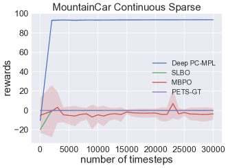
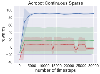
Figure 2: Episodic returns and success rates on MountainCar (top), Acrobot (bottom) environments with continuous action spaces, averaged over 4 random seeds. For the learning curve of HandEgg experiment, we refer back to Fig. 1. The solid line denotes the mean and the shaded area denotes one standard deviation. Note in the top plot the results of SLBO and PETS-GT almost overlap after the second iteration and thus the learning curve of SLBO is covered.

We first investigate how our algorithm mitigates the exploration issue faced by traditional MBRL algorithms with three continuous control and robotic environments in OpenAI Gym (Brockman et al., 2016). The first environment is the Mountain Car environment (Moore, 1990) with a continuous action space of $[-1,1]$. Upon every timestep, a small control cost is incurred, and the learner receives no reward until they reach the goal where they receive a reward of 100 and the episode terminates. The second environment is Acrobot (Sutton, 1996; Geramifard et al., 2015), and while the original action space is discrete, here we change the action space to continuous with range $[-1,1]$. We use the same reward scheme as in Mountain Car. The third environment is a hand manipulation task on the egg object (Plappert et al., 2018). We follow the original task design that incurs a constant penalty for not reaching the goal but we change the reward to 10 upon reaching the goal state. We remove the rotational perturbation but still keep the positional perturbation during goal sampling. This slightly relaxes the problem since our focus is on exploration issues instead of solving goal-conditioned RL problems and one algorithm is still required to learn the rotational dynamics by strategic exploration.

We observe that these three environments are very challenging to traditional MBRL algorithms: in the first two environments, because of the existence of the motor cost, one suboptimal policy is to just take actions with minimal motor costs. Thus the model will only be accurate around the initial states and never reach the goal state. For the manipulation environment, the huge state space and complex dynamics prohibit random exploration, which could require impractical numbers of samples to accurately capture the dynamics.

Here we compare with three MBRL baselines: a) PETS-GT (Chua et al., 2018) with CEM (Botev et al., 2013), and here we gives it the access to the ground truth dynamics. We also include baselines with moderate exploration power: b) SLBO (Luo et al., 2018) enforces entropy regularization during TRPO updates and adding Ornstein-Uhlunbeck noise while collecting samples. c) MBPO (Janner et al., 2019) uses SAC (Haarnoja et al., 2018) as the planner to encourage exploration. We plot the learning curves in Fig. 2. In the first two environments, while all the other baselines completely fail, Deep PC-MPL achieves the optimal performance within very few model updates. This indicates that with our constructed bonus, the planner has enough exploration power to reach the goal state with small numbers of samples. The results on the manipulation task also verify our hypothesis: with strategic exploration, our algorithm captures the dynamics in a reasonable number of samples and thus the planner learns to reach the goal while planning under the accurate model. However, with the same number of samples, the other baseline (SLBO) with random exploration could barely reach the goal state with the inaccurate dynamics model due to insufficient exploration.

	PETS-CEM	SLBO
Mean Rank	5.6/11	4/11
Median Rank	6/11	5/11
	Best MBBL	Deep PC-MLP (Ours)
Mean Rank	4/11	2.4/11
Median Rank	4/11	1.5/11

Table 1: The rankings of our algorithm and other baselines in the 10 benchmark environments in Table 2. The rankings are out of 11 algorithms (10 baselines from the benchmark paper plus Deep PC-MLP). We rank the algorithms descendingly based on their mean episodic returns for each task. We then take the average position in the ranking (from 1 to 11) across the 10 tasks as the mean rank and likewise for the median rank. Note here the best mean and median rank from the benchmark paper (denoted as Best MBBL) may not be the rank of the same algorithm.

	HalfCheetah	Hopper-ET	Walker2D-ET	Reacher	Ant
PETS-CEM	$2795.3\pm 879.9$	$129.3\pm 36.0$	$-2.5\pm 6.8$	$-15.1\pm 1.7$	$1165.5\pm 226.9$
SLBO	$1097.7\pm 166.4$	$805.7\pm 142.4$	$207.8\pm 108.7$	$-4.1\pm 0.1$	$718.1\pm 123.3$
Best MBBL	$3639.0\pm 1185.8$	$926.9\pm 154.1$	$312.5\pm 493.4$	$-4.1\pm 0.1$	$1852.1\pm 141.0$
Deep PC-MLP (Ours)	$3599.9\pm 662.6$	$1076.1\pm 378.6$	$1873.9\pm 927.0$	$-3.8\pm 0.2$	$1583.1\pm 903.6$
TRPO	$-12\pm 85.5$	$237.4\pm 33.5$	$229.5\pm 27.1$	$-10.1\pm 0.6$	$323.3\pm 24.9$
	Humanoid-ET	SlimHumanoid-ET	Swimmer	Swimmer-v0	Pendulum
PETS-CEM	$110.8\pm 91.0$	$355.1\pm 157.1$	$306.3\pm 37.3$	$22.1\pm 25.2$	$167.4\pm 53.0$
SLBO	$1377.0\pm 150.4$	$776.1\pm 252.5$	$125.2\pm 93.2$	$46.1\pm 18.4$	$173.5\pm 2.5$
Best MBBL	$1377.0\pm 150.4$	$1084.3\pm 77.0$	$336.3\pm 15.8$	$85.0\pm 98.9$	$177.3\pm 1.9$
DEEP PC-MLP (Ours)	$1775.5\pm 322.2$	$1521.0\pm 232.6$	$161.8\pm 167.8$	$26.1\pm 21.0$	$174.0\pm 2.4$
TRPO	$289.8\pm 5.2$	$281.3\pm 10.9$	$215.7\pm 10.4$	$37.9\pm 2.0$	$166.7\pm 7.3$

Table 2: Final performance for benchmark Mujoco locomotion and navigation tasks. The MBRL (top 4) algorithms are evaluated after 200k real world samples and the MFRL algorithm (TRPO) is evaluated after 1 million real world samples. All the results of the baselines (both model-based and model-free ones) are directly adopted from (Wang et al., 2019). We use the same 4 random seeds as in the benchmark paper while testing our algorithm and reporting the results. Here “ET” in the environment name denotes that the planner has access to the termination function, which is a common assumption in current MBRL algorithms (Janner et al., 2019; Rajeswaran et al., 2020). We use bold font to highlight the results of the algorithms with top 1 episodic rewards in each of the environments.

7.2 Dense Reward Environments

For dense reward environments, we follow the same setup as in the MBRL benchmark paper (Wang et al., 2019). We test Deep PC-MPL in 10 Mujoco (Todorov et al., 2012) locomotion and navigation environments. We report the final evaluation performance of our algorithm (after training with 200k real-world samples) in Table 2. For reference, we include the performances of PETS-CEM (Chua et al., 2018), SLBO (Luo et al., 2018), and the best MBRL algorithm in the benchmark paper for each corresponding environment (denoted as Best MBBL). We also include the evaluation result of our planner algorithm, TRPO, trained with 1 million real-world samples. Following the format in (Wang et al., 2019), we also provide the ranking of each algorithm in Table 1.

The results show that Deep PC-MPL achieves the best performances in 5 out of 10 environments, including the most challenging control environments such as Humanoid and Walker. This indicates that our exploration scheme helps boost the performances even under dense reward settings. Note that our algorithm uses the same set of hyperparameters for all 10 environments.

7.3 Reward Free Exploration

In this section, we investigate the performance of Deep PC-MLP in the context where there is no explicit reward signal. We test our algorithm in the high-dimensional AntMaze environment (shown in Fig. 1), following (Trott et al., 2019), but here the goal is to control the ant agent to explore as many distinct states in the U-shaped maze as possible. In this task, the agent receives no explicit rewards for reaching new states, but only small rewards are given for keeping the ant agent moving, which is irrelevant to the maze exploration task (algorithms without exploration ability tend to output agents running in a circle around the spawning point). We summarize the performance of our method in Fig. 3, where the results show that our method quickly covers the whole maze while random exploration completely fails to explore. We further visualize the trace map from different policies in the policy cover, which shows that different policies learn to explore different regions of the maze. The unification of the traces from the policies in the policy cover can provide a uniform coverage over the entire environment (see Fig. 1).

(a) Coverage Curve

(b) Policy 10

(c) Policy 30

(d) Policy 50

Figure 3: Visualization on AntMaze environment. (a): coverage curve of PC-MLP vs. random exploration. (b) Trace map from policy 10 from the policy cover. Yellow dots denote states in the earlier of the trajectories and purple dots denote later states in the trajectories. (c) Trace map from policy 30. (d) Trace map from policy 50.

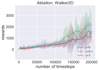
Figure 4: Ablation study: Comparison of different bonus coefficients in sparse reward environment MountainCar (top) and dense reward environment Walker2D (bottom). The results are averaged over 4 random seeds. The solid line denotes the mean and the shaded area denotes one standard deviation. In the first plot, note that the behaviors when $c=0$ and $c=1$ are identical thus the learning curves overlap.

7.4 Ablation Study on Bonus

Next, we investigate how the magnitude of the exploration bonus affects the performance of our algorithm. We control the amount of exploration by changing the bonus coefficient $c$ defined in Eq. 2 and we show the learning curves of different coefficient choices in Fig. 4.

For sparse reward environments such as Mountain Car, lacking exploration results in a suboptimal policy that takes actions that minimize the motor cost, which resembles the behaviors of the other baseline algorithms in section 7.1. If the bonus signal is not strong enough ($c=1$), we hypothesize that the control cost still dominates and thus it results in the same suboptimal policy with limited exploration around the initial states. For dense reward environments, existence of bonus ($c=0.1$) outperforms situation where there is no bonus ($c=0$). However, if the bonus signal is too strong ($c=1$), it will focus too much on exploration while ignoring exploitation.

7.5 Ablation Study: Vanishing Bonus

According to the construction of bonus, our algorithm will assign small bonuses to state-action pairs that are already visited. Theoretically, the bonuses of all state-action pairs will eventually converge to 0 after we fully explore the environment. In this section, we investigate the trend of the bonus empirically in the sparse reward environment MountainCar. Fig. 5 shows the curve of the bonus per timestep that the planner receives during the evaluation phase in the real-world environment. Here all hyperparameters are fixed as in the settings in section 7.1. We discover that the average bonus converges to near 0 quickly, indicating that our algorithm can finish fully exploring the environment within the very first few iterations.

Figure 5: Decay of bonus per timestep as Deep PC-MPL fully explores the Mountain Car environment. The results are collected on the same random seeds as in section 7.1.

8 Conclusion

In this paper, we introduce a new algorithm framework PC-MLP, which stands for Model Learning and Planning with Policy Cover for Exploration. We show that the same algorithm framework achieves polynomial sample complexity on both linear MDP and KNR models. Computation-wise, the algorithm uses a reward bonus and a black-box planner that optimizes the combination of the ground truth reward and the reward bonus inside the learned models.

Our algorithm is modular and has great flexibility to integrate with modern rich function approximators such as deep neural networks. We provide a practical instantiation of PC-MLP where we use a deep neural network to model transition dynamics and uses reward bonus based on random features either from RFF or from a fully connected layer of a randomly initialized neural network. Our bonus scheme is simple and is motivated by classic linear bandit theory and recent RL theory on models beyond tabular MDPs. Extensive empirical results indicate that our algorithm works well on exploration challenging tasks including a high-dimensional manipulation task and reward-free exploration. For a common continuous control benchmark where the dense reward is available, our algorithm still provides competitive results. Further ablation study indicates that even for dense reward settings, a mild amount of exploration is helpful.

Appendix A Sample Complexity Analysis of PC-MLP

In this section, we provide a detailed analysis for PC-MLP on both KNRs and Linear MDPs.

A.1 Model Learning from MLE

We consider a fixed episode $n$. The derived result here can be applied to all episodes via a union bound. We derive model’s generalization error under distribution $d^{\bm{\pi}_{n}}$ in terms of total variation distance. For linear MDPs, we can directly call Theorem 21 from (Agarwal et al., 2020b), which shows under realizability $P^{\star}\in\mathcal{P}$, the empirical maximizer of MLE directly enjoys the following generalization error.

Lemma 5 (MLE for linear MDPs (Theorem 21 from (Agarwal et al., 2020b))).

Fix $\delta\in(0,1)$, and assume $|\mathcal{P}|<\infty$ and $P^{\star}\in\mathcal{P}$. Consider $M$ samples with $(s_{i},a_{i})\sim d^{\bm{\pi}_{n}}$, and $s_{i}^{\prime}\sim P^{\star}(\cdot|s,a)$. Denote the empirical risk minimizer as $\widehat{P}_{n}=\mathop{\mathrm{argmax}}_{P\in\mathcal{P}}\sum_{i=1}^{M}\ln P(s_{i}^{\prime}|s_{i},a_{i})$. We have that with probability at least $1-\delta$,

$$\mathbb{E}_{s,a\sim d^{\bm{\pi}_{n}}}\left\|\widehat{P}_{n}(\cdot|s,a)-P^{\star}(\cdot|s,a)\right\|^{2}_{1}\leq{\frac{2\ln\left(\left\lvert\mathcal{P}\right\rvert/\delta\right)}{M}}.$$

For KNRs, we do not need to rely on the exact empirical risk minimization. Instead, we can use approximation optimization approach SGD here. Note that due to the Gaussian noise in the KNR model, we have that for a model $P_{W}$ with $W$ as the parameterization:

$$\ln P_{W}(s^{\prime}|s,a)=-\|W\phi(s,a)-s^{\prime}\|_{2}^{2}/\sigma^{2}+\ln(1/C),$$

where $C$ is the normalization constant for Gaussian distribution with zero mean and covariance matrix $\sigma^{2}I$. Hence gradient of the log-likelihood is equivalent to the gradient of the squared $\ell_{2}$ loss. Specifically, for approximately optimizing the empirical log-likelihood, we start with ${W}^{0}=0$, and perform SGD with ${W}^{i+1}=\prod_{W:\|W\|_{2}\leq F}\left({W}^{i}-\eta\left(W^{i}\phi(s_{i},a_{i})-s^{\prime}_{i}\right)\phi(s_{i},a_{i})^{\top}\right)$ and set $\widehat{W}_{n}=\frac{1}{M}\sum_{i=1}^{M}W^{i}$.

To use SGD’s result, we first need to bound all states $s^{\prime}$. The following lemma indicates that with high probability, the states have bounded norms.

Lemma 6.

In each episode, we generate M data points $\{s_{i},a_{i},s_{i}^{\prime}\}_{i=1}^{M}$ with $s_{i},a_{i}\sim d^{\bm{\pi}_{n}}$ and $s_{i}^{\prime}\sim\mathcal{N}\left(W^{\star}\phi(s_{i},a_{i}),\sigma^{2}I\right)$ with $\|W^{\star}\|_{2}\leq F$. With probability at least $1-\delta$, we have:

$$\left\|s_{i}^{\prime}\right\|_{2}\leq F+\sigma\sqrt{d_{s}\ln\left(d_{s}M/\delta\right)},\forall i\in[1,\dots,M].$$

Proof.

Denote $s_{i}^{\prime}=\epsilon_{i}+W^{\star}\phi(s_{i},a_{i})$ where $\epsilon_{i}\sim\mathcal{N}(0,\sigma^{2}I)$. We must have that for a fixed $i$ and dimension $j\in[d_{s}]$:

$$\mathbb{P}(|\epsilon_{i}[j]|\geq t)\leq\exp(-t^{2}/\sigma^{2}).$$

Take a union bound over all $i,j$, we have:

$$\mathbb{P}(\exists i,j,\text{ s.t. }|\epsilon_{i}[j]|\geq t)\leq d_{s}M\exp(-t^{2}/\sigma^{2}).$$

Set $d_{s}M\exp(-t^{2}/\sigma^{2})=\delta$, we get:

$$t=\sigma\sqrt{\ln\left(\frac{d_{s}M}{\delta}\right)}.$$

Hence with probability $1-\delta$, for $i,j$, we have:

$$\left\lvert\epsilon_{i}[j]\right\rvert\leq\sigma\sqrt{\ln\frac{d_{s}M}{\delta}}.$$

Hence, $\|s_{i}^{\prime}\|_{2}\leq\|W^{\star}\phi(s_{i},a_{i})\|_{2}+\|\epsilon_{i}\|_{2}\leq F+\sigma\sqrt{d_{s}\ln\left(\frac{d_{s}M}{\delta}\right)}$. ∎

Throughout this section, we assume the above event in Lemma 6 holds and we denote $F+\sigma\sqrt{d_{s}\ln\left(d_{s}M/\delta\right)}=B$ for notation simplicity .

Now we can call Lemma 16 (dimension-free SGD result) to conclude the following lemma.

Lemma 7 (MLE on KNRs).

With probability at least $1-\delta$, we have that:

$$\mathbb{E}_{s,a\sim d^{\bm{\pi}_{n}}}\left[\left\|\widehat{W}_{n}\phi(s,a)-W^{\star}\phi(s,a)\right\|_{2}^{2}\right]\leq\frac{3(F^{2}+FB)\ln(1/\delta)}{\sqrt{M}},$$

where $B=F+\sigma\sqrt{d_{s}\ln\left(\frac{2d_{s}M}{\delta}\right)}$.

Proof.

Lemma 6 states that with probability $1-\delta/2$, we have that $\|s_{i}^{\prime}\|_{2}\leq B$ for all $i\in[1,\dots,M]$. Condition on this event, we call Lemma 16 and using the fact that $\|W^{\star}\|_{2}\leq\|W^{\star}\|_{F}\leq F$, we get that with probability at least $1-\delta/2$,

$$\mathbb{E}_{s,a\sim d^{\bm{\pi}_{n}}}\left[\left\|\widehat{W}_{n}\phi(s,a)-W^{\star}\phi(s,a)\right\|_{2}^{2}\right]\leq\frac{3(F^{2}+FB)\ln(2/\delta)}{\sqrt{M}}$$

The total probability of failure is $\delta$.

This concludes the proof. ∎

A.2 Optimism at the Starting State

We denote $b_{n}(s,a)$ using $\Sigma_{n}$ as follows:

$$b_{n}(s,a)=\min\left\{c\sqrt{\phi(s,a)^{\top}\Sigma_{n}^{-1}\phi(s,.a)},\;H\right\}.$$

Recall that the reward bonus in the algorithm is defined with respect to $\widehat{\Sigma}_{n}$ in Eq. 2. We will link $b_{n}$ and $\widehat{b}_{n}$ later in the analysis.

The bonus is related to the uncertainty in the model. Consider any policy $\pi$, reward bonus $b_{n}$ in the form of Eq. 2, and any model $\widehat{P}\in\mathcal{P}$. Denote $\widehat{V}^{\pi}_{r+b_{n};h}$ as the value function at time step $h$ under policy $\pi$ in model $\widehat{P}$ and reward $r+b_{n}$. Note that $r(s,a)+b_{n}(s,a)\in[0,H+1]$, we have $\|\widehat{V}^{\pi}_{r+b_{n},h}\|_{\infty}\leq H^{2}$ for any $h$.

Lemma 8 (Optimism in Linear MDPs).

Assume the following condition hold for all $n\in[1,\dots,N]$:

$$\mathbb{E}_{s,a\sim d^{\bm{\pi}_{n}}}\|\widehat{P}_{n}(\cdot|s,a)-P^{\star}(\cdot|s,a)\|^{2}_{1}\leq\epsilon_{stat}\in\mathbb{R}^{+},\forall n.$$

Set $c=H\sqrt{\left(\lambda d+N\epsilon_{stat}\right)}$, and assume $b_{n}(s,a)\leq\widehat{b}_{n}(s,a)\leq 4b_{n}(s,a)$ holds for all $n$. Then, we have that for any $n$:

$$\widehat{V}^{\pi_{n+1}}_{r+\widehat{b}_{n};0}(s_{0})\geq\max_{\pi\in\Pi}V^{\pi}_{0}(s_{0}).$$

Proof.

We denote $\pi^{\star}=\mathop{\mathrm{argmax}}_{\pi\in\Pi}V^{\pi}_{0}(s_{0})$. We consider $\pi^{\star}$ specifically. Without loss of generality, we denote $\widehat{V}^{\pi}_{r+\hat{b}_{n};H}(s)=V^{\pi}_{H}(s)=0$ for all $s\in{\mathcal{S}}$. Thus, for $h=H$, we have $\widehat{V}^{\pi^{\star}}_{r+\hat{b}_{n};H}(s)\geq V^{\pi^{\star}}_{H}(s),\forall s$.

Assume that at time step $h+1$, we have $\widehat{V}^{\pi^{\star}}_{r+\hat{b}_{n};h+1}(s)\geq V^{\pi^{\star}}_{h+1}(s),\forall s$. Now we move on to prove this also holds at time step $h$. Denote $a^{\star}=\pi^{\star}(s)$. Also we define $\Sigma_{n}=\sum_{i=1}^{n}\Sigma_{\pi_{n}}+\lambda I$.

$$\widehat{V}^{\pi^{\star}}_{r+\hat{b}_{n};h}(s)-{V}^{\pi^{\star}}_{h}(s) =r(s,a^{\star})+\widehat{b}_{n}(s,a^{\star})+\mathbb{E}_{s^{\prime}\sim\widehat{P}^{n}(\cdot|s,a^{\star})}\widehat{V}^{\pi^{\star}}_{r+\hat{b}_{n};h+1}(s^{\prime})-\left(r(s,a^{\star})+\mathbb{E}_{s^{\prime}\sim P^{\star}(\cdot|s,a^{\star})}V^{\pi^{\star}}_{h+1}(s^{\prime})\right)$$

$$\geq b_{n}(s,a^{\star})+\left(\mathbb{E}_{s^{\prime}\sim\widehat{P}^{n}(\cdot|s,a^{\star})}{V}^{\pi^{\star}}_{h+1}(s^{\prime})-\mathbb{E}_{s^{\prime}\sim P^{\star}(\cdot|s,a^{\star})}V_{h+1}^{\pi^{\star}}(s^{\prime})\right)$$

$$=b_{n}(s,a^{\star})+\left((\widehat{\mu}_{n}-\mu^{\star})\phi(s,a^{\star})\right)\cdot V^{\pi^{\star}}_{h+1}$$

We bound $\left((\widehat{\mu}_{n}-\mu^{\star})\phi(s,a)\right)\cdot V^{\pi^{\star}}_{h+1}$ below.

$$\left\lvert\left((\widehat{\mu}_{n}-\mu^{\star})\phi(s,a)\right)\cdot V^{\pi^{\star}}_{h+1}\right\rvert^{2}\leq\|\phi(s,a)\|^{2}_{\Sigma^{-1}_{n}}\left\|\left(\widehat{\mu}_{n}-\mu^{\star}\right)^{\top}V^{\pi^{\star}}_{h+1}\right\|^{2}_{\Sigma_{n}}$$

$$=\|\phi(s,a)\|^{2}_{\Sigma^{-1}_{n}}\left(\lambda\left\|\left(\widehat{\mu}_{n}-\mu^{\star}\right)^{\top}V^{\pi^{\star}}_{h+1}\right\|_{2}^{2}+n\mathbb{E}_{s,a\sim d^{\bm{\pi}_{n}}}\left(\phi(s,a)^{\top}\left(\widehat{\mu}_{n}-\mu^{\star}\right)^{\top}V^{\pi^{\star}}_{h+1}\right)^{2}\right)$$

$$\leq\|\phi(s,a)\|^{2}_{\Sigma^{-1}_{n}}\left(\lambda\left\|\left(\widehat{\mu}_{n}-\mu^{\star}\right)^{\top}V^{\pi^{\star}}_{h+1}\right\|_{2}^{2}+nH^{2}\mathbb{E}_{s,a\sim d^{\bm{\pi}_{n}}}\|\widehat{P}_{n}(\cdot|s,a)-P^{\star}(\cdot|s,a)\|^{2}_{1}\right)$$

$$\leq\|\phi(s,a)\|^{2}_{\Sigma^{-1}_{n}}\left(\lambda H^{2}d+nH^{2}\mathbb{E}_{s,a\sim d^{\bm{\pi}_{n}}}\|\widehat{P}_{n}(\cdot|s,a)-P^{\star}(\cdot|s,a)\|^{2}_{1}\right)$$

$$\leq\left(\lambda H^{2}d+nH^{2}\epsilon_{stat}\right)\|\phi(s,a)\|^{2}_{\Sigma_{n}^{-1}}\leq c^{2}\|\phi(s,a)\|^{2}_{\Sigma_{n}^{-1}}.$$

Thus, we get that:

$$\widehat{V}^{\pi^{\star}}_{r+\hat{b}_{n};h}(s)-{V}^{\pi^{\star}}_{h+1}(s)\geq b_{n}(s,a^{\star})-c\|\phi(s,a^{\star})\|_{\Sigma_{n}^{-1}}=0.$$

Note that the above holds for any $s$. Thus via induction, we conclude that at $h=0$, we have $\widehat{V}^{\pi^{\star}}_{r+\hat{b}_{n};0}(s_{0})\geq V^{\pi^{\star}}_{0}(s_{0})$. Using the fact that $\pi_{n+1}=\mathop{\mathrm{argmax}}_{\pi\in\Pi}\widehat{V}^{\pi}_{r+\hat{b}_{n};0}(s_{0})$, we conclude the proof. ∎

Lemma 9 (Optimism in KNRs).

Assume the following condition hold for all $n\in[1,\dots,N]$:

$$\mathbb{E}_{s,a\sim d^{\bm{\pi}_{n}}}\left\|\widehat{W}_{n}\phi(s,a)-W^{\star}\phi(s,a)\right\|^{2}_{2}\leq\epsilon_{stat},\forall n,$$

Set $c=\frac{1}{\sigma}{H\sqrt{\lambda 4F^{2}+N\epsilon_{stat}}}$, and assume that $b_{n}(s,a)\leq\widehat{b}_{n}(s,a)\leq 4b_{n}(s,a)$ holds for all $n$. we have that for any $n$:

$$\widehat{V}^{\pi_{n+1}}_{r+\hat{b}_{n};0}(s_{0})\geq\max_{\pi\in\Pi}V^{\pi}_{0}(s_{0}).$$

Proof.

For any $n$, the condition in the lemma implies that:

$$\sum_{i=1}^{n}\mathbb{E}_{s,a\sim d^{\pi_{i}}}\left\|\widehat{W}_{n}\phi(s,a)-W^{\star}\phi(s,a)\right\|^{2}_{2}=\mathop{\mathrm{tr}}\left(\left(\widehat{W}_{n}-W^{\star}\right)\sum_{i=1}^{n}\Sigma_{\pi_{i}}\left(\widehat{W}_{n}-W^{\star}\right)^{\top}\right)\leq n\epsilon_{stat}$$

Note that $\Sigma_{n}=\sum_{i=1}^{n}\Sigma_{\pi_{i}}+\lambda I$, we have that:

$$\left\|\left(\widehat{W}_{n}-W^{\star}\right)\Sigma_{n}^{1/2}\right\|_{2}^{2}\leq\mathop{\mathrm{tr}}\left(\left(\widehat{W}_{n}-W^{\star}\right)\Sigma_{n}\left(\widehat{W}_{n}-W^{\star}\right)^{\top}\right)\leq n\epsilon_{stat}+\lambda 4F^{2},$$

where we use the norm bound that $\|\widehat{W}_{n}\|^{2}_{F}\leq F^{2},\|W^{\star}\|_{F}^{2}\leq F^{2}$.

Similarly, we can use induction to prove optimism. Assume $\widehat{V}^{\pi^{\star}}_{r+\hat{b}_{n};h+1}(s)\geq V^{\pi^{\star}}_{h+1}(s)$ for all $s$. For any $s$, denote $a^{\star}=\pi^{\star}(s)$, we have:

$$\widehat{V}^{\pi^{\star}}_{r+\hat{b}_{n};h}(s)-V^{\pi^{\star}}_{h}(s) \geq b_{n}(s,a^{\star})+\left(\mathbb{E}_{s^{\prime}\sim\widehat{P}^{n}(\cdot|s,a^{\star})}{V}^{\pi^{\star}}_{h+1}(s^{\prime})-\mathbb{E}_{s^{\prime}\sim P^{\star}(\cdot|s,a^{\star})}V_{h+1}^{\pi^{\star}}(s^{\prime})\right)$$

$$\geq b_{n}(s,a^{\star})-\left\|\widehat{P}_{n}(\cdot|s,a^{\star})-P^{\star}(\cdot|s,a^{\star})\right\|_{1}\|V^{\pi^{\star}}_{h+1}\|_{\infty}$$

$$\geq b_{n}(s,a^{\star})-\frac{H}{\sigma}\left\|\left(\widehat{W}_{n}-W^{\star}\right)\phi(s,a^{\star})\right\|_{2}$$

$$\geq b_{n}(s,a^{\star})-\frac{H}{\sigma}\left\|\widehat{W}_{n}-W^{\star}\right\|_{\Sigma_{n}}\left\|\phi(s,a^{\star})\right\|_{\Sigma_{n}^{-1}}$$

$$\geq b_{n}(s,a^{\star})-\frac{H\sqrt{n\epsilon_{stat}+\lambda 4F^{2}}}{\sigma}\|\phi(s,a^{\star})\|_{\Sigma_{n}^{-1}}\geq 0,$$

due to the set up of $c$. Similar via induction, this concludes the proof. ∎

A.3 Regret Upper Bound

Below we consider bounding $\sum_{n=1}^{N}\left(J(\pi^{\star};P^{\star})-J(\pi_{n};P^{\star})\right)$ using optimism we proved in the section above.

Lemma 10 (Regret bound in linear MDPs).

Assuming all conditions in Lemma 8 holds. We have:

$$\sum_{n=1}^{N}\left(J(\pi^{\star};r,P^{\star})-J(\pi_{n};r,P^{\star})\right)\leq 6H^{2}\sum_{n=1}^{N-1}\mathbb{E}_{s,a\sim d^{\pi_{n+1}}}\left[b_{n}(s,a)\right]+H.$$

Proof.

Since the condition in Lemma 8 holds, we have that for all $n$, optimism holds, i.e., $J(\pi_{n+1};r+\widehat{b}_{n},\widehat{P}_{n})\geq J(\pi^{\star};r,P^{\star})$. Hence, together with the simulation lemma (Lemma 19) we have:

$$J(\pi^{\star};r,P^{\star})-J(\pi_{n+1};r,P^{\star}) \leq J(\pi_{n+1};r+\widehat{b}_{n},\widehat{P}_{n})-J(\pi_{n+1};r,P^{\star})$$

$$=\sum_{h=0}^{H-1}\mathbb{E}_{s,a\sim d^{\pi_{n+1}}_{h}}\left[\widehat{b}_{n}(s,a)+\left(\widehat{P}_{n}(\cdot|s,a)-P^{\star}(\cdot|s,a)\right)\cdot\widehat{V}^{\pi_{n+1}}_{r+\hat{b}_{n};h+1}\right]$$

$$\leq\sum_{h=0}^{H-1}\mathbb{E}_{s,a\sim d^{\pi_{n+1}}_{h}}\left[4{b}_{n}(s,a)+\left(\widehat{P}_{n}(\cdot|s,a)-P^{\star}(\cdot|s,a)\right)\cdot\widehat{V}^{\pi_{n+1}}_{r+\hat{b}_{n};h+1}\right].$$

Note that $\|\widehat{V}^{\pi}_{r+\hat{b};h}\|_{\infty}\leq H^{2}$ for any $\pi,h,n$. Following similar derivation in the proof of Lemma 8, we have:

$$\left\lvert\left((\widehat{\mu}_{n}-\mu^{\star})\phi(s,a)\right)\cdot\widehat{V}^{\pi_{n+1}}_{r+b_{n};h+1}\right\rvert \leq\min\left\{\|\phi(s,a)\|_{\Sigma_{n}^{-1}}\sqrt{\left(\lambda H^{4}d+nH^{4}\epsilon_{stat}\right)},2H^{2}\right\}$$

$$\leq 2H\min\left\{H\sqrt{\lambda d+N\epsilon_{stat}}\cdot\left\|\phi(s,a)\right\|_{\Sigma_{n}^{-1}},\;H\right\}=2Hb_{n}(s,a).$$

Note that the regret at the first policy $\pi_{1}$ is at most $H$. This concludes the proof. ∎

Lemma 11 (Regret bound in KNRs).

Assuming all conditions in Lemma 9 holds. We have:

$$\sum_{n=1}^{N}\left(J(\pi^{\star};r,P^{\star})-J(\pi_{n};r,P^{\star})\right)\leq 5H^{2}\sum_{n=1}^{N-1}\mathbb{E}_{s,a\sim d^{\pi_{n+1}}}\left[b_{n}(s,a)\right]+H.$$

Proof.

Again, via simulation lemma and optimism, we have:

$$J(\pi^{\star};r,P^{\star})-J(\pi_{n+1};r,P^{\star}) \leq\sum_{h=0}^{H-1}\mathbb{E}_{s,a\sim d^{\pi_{n+1}}_{h}}\left[\widehat{b}_{n}(s,a)+\left(\widehat{P}_{n}(\cdot|s,a)-P^{\star}(\cdot|s,a)\right)\cdot\widehat{V}^{\pi_{n+1}}_{r+b_{n};h+1}\right]$$

$$\leq\sum_{h=0}^{H-1}\mathbb{E}_{s,a\sim d^{\pi_{n+1}}_{h}}\left[4{b}_{n}(s,a)+\left(\widehat{P}_{n}(\cdot|s,a)-P^{\star}(\cdot|s,a)\right)\cdot\widehat{V}^{\pi_{n+1}}_{r+b_{n};h+1}\right]$$

Following the derivation in the proof of Lemma 9, we have:

$$\left\lvert\left(\widehat{P}_{n}(\cdot|s,a)-P^{\star}(\cdot|s,a)\right)\cdot\widehat{V}^{\pi_{n+1}}_{r+b_{n};h+1}\right\rvert\leq\frac{H^{2}\sqrt{n\epsilon_{stat}+\lambda 4F^{2}d_{s}}}{\sigma}\|\phi(s,a)\|_{\Sigma_{n}^{-1}}=Hb_{n}(s,a).$$

Combine the above two inequalities, we conclude the proof. ∎

Recall the definition of information gain, $\mathcal{I}_{N}(\lambda)=\max_{\pi_{1},\dots,\pi_{N}}\ln\det\left(I+\frac{1}{\lambda}\sum_{n=1}^{N}\Sigma_{\pi_{n}}\right)$.

Lemma 12.

For any sequence of policies $\pi_{1},\dots,\pi_{n}$, with $\Sigma_{n}=\sum_{i=1}^{n}\Sigma_{\pi_{n}}$ and $b_{n}(s,a)\leq c\sqrt{\phi(s,a)^{\top}\Sigma_{n}^{-1}\phi(s,a)}$, we have that:

$$\sum_{n=1}^{N-1}\mathbb{E}_{s,a\sim d^{\pi_{n+1}}}b_{n}(s,a)\leq c\sqrt{2N\mathcal{I}_{N}(\lambda)}.$$

When $\phi\in\mathbb{R}^{d}$, we have:

$$\sum_{n=1}^{N-1}\mathbb{E}_{s,a\sim d^{\pi_{n+1}}}b_{n}(s,a)\leq c\sqrt{2Nd\ln\left(1+N/\lambda\right)}.$$

Proof.

Starting from the definition of $b_{n}$, we have:

$$\sum_{n=1}^{N-1}\mathbb{E}_{s,a\sim d^{\pi_{n+1}}}b_{n}(s,a) \leq c\sum_{n=1}^{N-1}\mathbb{E}_{s,a\sim d^{\pi_{n+1}}}\sqrt{\phi(s,a)^{\top}\Sigma_{n}^{-1}\phi(s,a)}\leq c\sqrt{N}\sqrt{\sum_{n=1}^{N-1}\mathbb{E}_{s,a\sim d^{\pi_{n+1}}}{\phi(s,a)^{\top}\Sigma_{n}^{-1}\phi(s,a)}}$$

$$=c\sqrt{N}\sqrt{\sum_{n=1}^{N-1}\mathop{\mathrm{tr}}\left(\Sigma_{\pi_{n+1}}\Sigma_{n}^{-1}\right)}\leq c\sqrt{2N\ln\left(\det(\Sigma_{N})/\det(\lambda I)\right)}$$

Here in the second inequality, we use Cauchy-Schwartz inequality, in the third inequality, we use Lemma 18.

If $\phi\in\mathbb{R}^{d}$, we have that:

$$\sqrt{N\ln(\det(\Sigma_{N})/\det(\lambda I))}\leq\sqrt{Nd\ln(1+N/\lambda)},$$

where we use $\|\phi(s,a)\|_{2}\leq 1$.

This concludes the proof. ∎

A.4 Concluding the Sample Complexity Calculation

Before concluding the final sample complexity, we need to link $\widehat{\Sigma}_{n}$ to $\Sigma_{n}$, as our reward bonus in the algorithm is defined in terms of the empirical estimate $\widehat{\Sigma}_{n}$.

Lemma 13 (Relating $\widehat{b}_{n}$ and $b_{n}$).

With probability at least $1-\delta$, for all $n\in[1,\dots,N]$, we have:

$$b_{n}(s,a)\leq\widehat{b}_{n}(s,a)\leq 4b_{n}(s,a),\forall s,a.$$

Proof.

The proof uses Lemma 20. Under Lemma 20, we have:

$$\min\left\{c\sqrt{\phi(s,a)^{\top}\widehat{\Sigma}^{-1}_{n}\phi(s,a)},H\right\}\leq\min\left\{c\sqrt{2}\sqrt{\phi(s,a)^{\top}{\Sigma}^{-1}_{n}\phi(s,a)},H\right\}$$

$$\leq\sqrt{2}\min\left\{c\sqrt{\phi(s,a)^{\top}{\Sigma}^{-1}_{n}\phi(s,a)},H\right\}=\sqrt{2}b_{n}(s,a).$$

and

$$b_{n}(s,a)/\sqrt{2}=\min\left\{c\sqrt{\phi(s,a)^{\top}\Sigma_{n}^{-1}\phi(s,a)},H\right\}/\sqrt{2}$$

$$\leq\min\left\{c\sqrt{(1/2)\phi(s,a)^{\top}\Sigma_{n}^{-1}\phi(s,a)},H\right\}\leq\min\left\{c\sqrt{\phi(s,a)^{\top}\widehat{\Sigma}_{n}^{-1}\phi(s,a)},H\right\},$$

Note that $\widehat{b}_{n}(s,a)=2\min\{c\sqrt{(1/2)\phi(s,a)^{\top}\widehat{\Sigma}_{n}^{-1}\phi(s,a)},H\}$, we have that:

$$b_{n}(s,a)/\sqrt{2}\leq\widehat{b}_{n}(s,a)/2\leq\sqrt{2}b_{n}(s,a),$$

which concludes the proof. ∎

In high level, from Lemma 10, Lemma 11, and Lemma 12 we know that after $N$ iterations, we have:

$$\max_{i\in[1,\dots,N]}J(\pi_{i};r,P^{\star})\geq J(\pi^{\star};r,P^{\star})-\frac{10H^{2}c}{\sqrt{N}}\sqrt{d\ln(1+N/\lambda)}.$$

Hence, to ensure we get an $\epsilon$ near optimal policy, we just need to set $N$ large enough such that $\frac{10H^{2}c}{\sqrt{N}}\sqrt{d\ln(1+N/\lambda)\ln}\approx\epsilon$ and to do so, we need to control $M$ in order to make $c$ scale as a constant.

A.4.1 Concluding for Linear MDPs

Theorem 14 (Sample Complexity for Linear MDPs).

Set $\delta\in(0,0.5)$ and $\epsilon\in(0,1)$. There exists a set of hyper-parameters,

$$N=\frac{80H^{6}d^{2}}{\epsilon^{2}}\ln\left(\frac{40H^{6}d^{2}}{\epsilon^{2}}\right),\quad M=2N\ln\left(|\mathcal{P}|N/\delta\right),\quad c=H\sqrt{d+1},\quad K=32N^{2}\ln\left(8Nd/\delta\right),$$

such that with probability at least $1-2\delta$, PC-MLP returns a policy $\widehat{\pi}$ such that:

$$J(\hat{\pi};r,P^{\star})\geq\max_{\pi\in\Pi}J(\pi;r,P^{\star})-\epsilon,$$

with number of samples

$$O\left(\frac{H^{18}d^{6}}{\epsilon^{6}}\cdot\ln\left(\frac{|\mathcal{P}|H^{6}d^{2}}{\epsilon^{2}\delta}\ln\left(\frac{H^{6}d^{2}}{\epsilon^{2}}\right)\right)\ln^{3}\left(\frac{H^{6}d^{2}}{\epsilon^{2}}\right)\right).$$

Ignoring log terms, we get the sample complexity scales in the order of $\widetilde{O}\left(\frac{H^{18}d^{6}}{\epsilon^{6}}\right)$.

The above theorem verifies Theorem 4

Proof.

From Lemma 8, we know that:

$$c=H\sqrt{d+N\epsilon_{stat}},$$

where we have set $\lambda=1$ explicitly. Also from Lemma 5, we know that with probability at least $1-\delta$,

$$\epsilon_{stat}=\frac{2\ln(|\mathcal{P}|N/\delta)}{M}.$$

We set $M$ large enough such that $N\epsilon_{stat}=1$. To achieve this, it is easy to verify that it is enough to set $M=2N\ln(|\mathcal{P}|N/\delta)$. As $d\geq 1$, we immediately have that $c\leq 2H\sqrt{d}$ in this case.

To achieve $\epsilon$ approximation error, we set $N$ big enough such that:

$$\frac{10H^{2}c}{\sqrt{N}}\sqrt{d\ln(1+N/\lambda)\ln}\leq\epsilon.$$

Using $c=2H\sqrt{d}$, we get:

$$\frac{20H^{3}{d}}{\sqrt{N}}\sqrt{\ln(1+N)}\leq\epsilon.$$

We can verify that the above inequality holds when we set:

$$N=\frac{80H^{6}d^{2}}{\epsilon^{2}}\ln\left(\frac{40H^{6}d^{2}}{\epsilon^{2}}\right).$$

Hence, the total number of samples we use for estimating models during $N$ epsilons is bounded as:

$$N\times M=2N^{2}\ln(|\mathcal{P}|N/\delta)\leq\frac{H^{12}d^{4}}{\epsilon^{4}}\cdot 12800\ln^{2}\left(\frac{40H^{6}d^{2}}{\epsilon^{2}}\right)\ln\left(\frac{80H^{6}d^{2}|\mathcal{P}|}{\epsilon^{2}\delta}\ln\left(\frac{40H^{6}d^{2}}{\epsilon^{2}}\right)\right).$$

We also need to count the total number of samples used to estimate the covariance matrix $\widehat{\Sigma}_{n}$ for all $n$. From Lemma 20. The number is bounded as:

$$K\cdot N=32N^{3}\ln\left(8Nd/\delta\right)=\frac{H^{18}d^{6}}{\epsilon^{6}}\cdot(32\times 80^{3})\ln^{3}\left(\frac{40H^{6}d^{2}}{\epsilon^{2}}\right)\ln\left(\frac{640H^{6}d^{3}}{\epsilon^{2}\delta}\ln\left(\frac{40H^{6}d^{2}}{\epsilon^{2}}\right)\right).$$

The total number of samples is $N\times M+N\times K$, which after rearranging terms, we get:

$$NM+NK\leq\frac{H^{18}d^{6}}{\epsilon^{6}}\cdot\ln\left(\frac{640H^{6}d^{2}|\mathcal{P}|}{\epsilon^{2}\delta}\ln\left(\frac{40H^{6}d^{2}}{\epsilon^{2}}\right)\right)\ln^{3}\left(\frac{40H^{6}d^{2}}{\epsilon^{2}}\right)\cdot(60\times 80^{3}).$$

We conclude here by noting that the total failure probability is at most $2\delta$. ∎

A.4.2 Concluding for KNRs

Theorem 15 (Sample Complexity for KNRs).

Set $\delta\in(0,0.5)$ and $\epsilon\in(0,1)$. There exists a set of hyper-parameters,

$$N=\Theta\left(\frac{H^{6}F^{2}d_{s}d}{\sigma^{2}\epsilon^{2}}\ln\left(\frac{H^{6}F^{2}d_{s}d}{\sigma^{2}\epsilon^{2}}\right)\right),\quad M=\Theta\left(N^{2}(F^{2}+FB)^{2}\ln^{2}\left(\frac{N}{\delta}\right)\right),$$

$$c=\Theta\left(\frac{H}{\sigma}\sqrt{d+1}\right),\quad K=32N^{2}\ln\left(8Nd/\delta\right),$$

such that with probability at least $1-2\delta$, PC-MLP returns a policy $\widehat{\pi}$ such that:

$$J(\hat{\pi};r,P^{\star})\geq\max_{\pi\in\Pi}J(\pi;r,P^{\star})-\epsilon,$$

with number of samples

$$O\left(\frac{H^{18}d^{3}d_{s}^{3}}{\sigma^{6}\epsilon^{6}}\cdot\left(F^{10}+\sigma^{2}F^{8}d_{s}\right)\nu\right),$$

where $\nu$ only contains log terms,

$$\nu =\ln^{2}\left(\frac{N}{\delta}\right)\ln\left(\frac{2d_{s}N}{\delta}\right)+\ln\left(\left(8F^{4}+9\sigma^{2}F^{2}d_{s}\ln\left(\frac{2d_{s}N}{\delta}\right)\right)\ln^{2}\left(\frac{N}{\delta}\right)N^{2}+18\sigma^{2}F^{2}d_{s}\right)$$

$$\qquad+\ln^{3}\left(\frac{6400H^{6}F^{2}d_{s}d}{\sigma^{2}\epsilon^{2}}\right)\ln\left(Nd/\delta\right).$$

Ignoring log terms, we get sample complexity scales in the order $\widetilde{O}\left(\frac{H^{18}d^{3}d_{s}^{3}}{\sigma^{6}\epsilon^{6}}\cdot\left(F^{10}+\sigma^{2}F^{8}d_{s}\right)\right)$.

The above theorem verifies Theorem 3

Proof.

The proof is similar to the proof of Theorem 14. From Lemma 9, we know that $c\leq\frac{4H}{\sigma}\sqrt{\lambda F^{2}d_{s}/\sigma^{2}+N\epsilon_{stat}/\sigma^{2}}$. Also from Lemma 7, we know that

$$\epsilon_{stat}=\frac{3(F^{2}+FB)\ln(N/\delta)}{\sqrt{M}},$$

with $B=F+\sigma\sqrt{d_{s}\ln(2d_{s}NM/\delta)}$, for all $n$. We set $M$ such that $N\epsilon_{stat}=1$. This gives us that:

$$M\geq 9N^{2}(F^{2}+FB)^{2}\ln^{2}\left(\frac{N}{\delta}\right).$$

Solve for $M$, we can verify that it suffices to set $M$ as:

$$M =\left(8F^{4}+9\sigma^{2}F^{2}d_{s}\ln\left(\frac{2d_{s}N}{\delta}\right)\right)\ln^{2}\left(\frac{N}{\delta}\right)N^{2}$$

$$\quad+18\sigma^{2}F^{2}d_{s}\ln\left(\left(8F^{4}+9\sigma^{2}F^{2}d_{s}\ln\left(\frac{2d_{s}N}{\delta}\right)\right)\ln^{2}\left(\frac{N}{\delta}\right)N^{2}+18\sigma^{2}F^{2}d_{s}\right)$$

This gives us $c=\frac{8H}{\sigma}\sqrt{F^{2}d_{s}}$.

Similarly, we will set $N$ such that $\frac{10H^{2}c}{\sqrt{N}}\sqrt{d\ln(1+N/\lambda)}\leq\epsilon$. With $c=\frac{8H}{\sigma}\sqrt{F^{2}d_{s}}$, we get:

$$\frac{80H^{3}\sqrt{F^{2}d_{s}}}{\sigma\sqrt{N}}\sqrt{d\ln(1+N/\lambda)}\leq\epsilon$$

We can verify that it suffices to set $N$ as:

$$N=\frac{12800H^{6}F^{2}d_{s}d}{\sigma^{2}\epsilon^{2}}\ln\left(\frac{6400H^{6}F^{2}d_{s}d}{\sigma^{2}\epsilon^{2}}\right)$$

Thus the total number of samples used for model learning is upper bounded as:

$$NM =O\left(N^{3}\left(F^{4}+\sigma^{2}F^{2}d_{s}\right)\ln^{2}\left(\frac{N}{\delta}\right)\ln\left(\frac{2d_{s}N}{\delta}\right)\right)$$

$$\qquad+O\left(N\sigma^{2}F^{2}d_{s}\cdot\ln\left(\left(8F^{4}+9\sigma^{2}F^{2}d_{s}\ln\left(\frac{2d_{s}N}{\delta}\right)\right)\ln^{2}\left(\frac{N}{\delta}\right)N^{2}+18\sigma^{2}F^{2}d_{s}\right)\right)$$

$$=O\left(\nu\frac{H^{18}d^{3}d_{s}^{3}F^{6}(F^{4}+\sigma^{2}F^{2}d_{s})}{\sigma^{6}\epsilon^{6}}\right),$$

where $v$ only contains log terms, i.e.,

$$\nu=\ln^{2}\left(\frac{N}{\delta}\right)\ln\left(\frac{2d_{s}N}{\delta}\right)+\ln\left(\left(8F^{4}+9\sigma^{2}F^{2}d_{s}\ln\left(\frac{2d_{s}N}{\delta}\right)\right)\ln^{2}\left(\frac{N}{\delta}\right)N^{2}+18\sigma^{2}F^{2}d_{s}\right).$$

We also need to count the total number of samples used to estimate the covariance matrix $\widehat{\Sigma}_{n}$ for all $n$. From Lemma 20. The number is bounded as:

$$K\cdot N=O\left(N^{3}\ln\left(Nd/\delta\right)\right)=O\left(\nu_{1}\cdot\frac{H^{18}F^{6}d_{s}^{3}d^{3}}{\sigma^{6}\epsilon^{6}}\right)$$

where $\nu_{1}$ only contains log terms, i.e.,

$$\nu_{1}=\ln^{3}\left(\frac{6400H^{6}F^{2}d_{s}d}{\sigma^{2}\epsilon^{2}}\right)\ln\left(Nd/\delta\right).$$

Combine the two terms, we can conclude that:

$$KN+KM=O\left(\frac{H^{18}d^{3}d_{s}^{3}}{\sigma^{6}\epsilon^{6}}\cdot\left(F^{10}+\sigma^{2}F^{8}d_{s}\right)\left(\nu+\nu_{1}\right)\right).$$

∎

Appendix B Auxiliary Lemmas

Lemma 16 (Dimension-free SGD (Lemma G.1 from (Agarwal et al., 2020a))).

Consider the following learning process. Initialize $W_{1}=\mathbf{0}$. For $i=1,\dots,N$, draw $x_{i},y_{i}\sim\nu$, $\|y_{i}\|_{2}\leq B$, $\|x_{i}\|\leq 1$; Set $W_{i+1}=\prod_{\mathcal{W}:=\{W:\|W\|_{2}\leq F\}}\left(W_{i}-\eta_{i}\left(W_{i}x_{i}-y_{i}\right)x_{i}^{\top}\right)$ with $\eta_{i}=(F^{2})/((F+B)\sqrt{N})$. Set $\widehat{W}=\frac{1}{N}\sum_{i=1}^{N}W_{i}$, we have that with probability at least $1-\delta$:

$$\mathbb{E}_{x\sim\nu}\left[\left\|\widehat{W}\cdot x-\mathbb{E}\left[y|x\right]\right\|_{2}^{2}\right]\leq\mathbb{E}_{x\sim\nu}\left[\left\|W^{\star}\cdot x-\mathbb{E}\left[y|x\right]\right\|_{2}^{2}\right]+\frac{R\sqrt{\ln(1/\delta)}}{\sqrt{N}},$$

with any $W^{\star}$ such that $\|W^{\star}\|_{2}\leq F$ and $R=3(F^{2}+FB)$.

Lemma 17 (Total Variation Distance between Two Gaussians).

Given two Gaussian distributions $P_{1}=\mathcal{N}(\mu_{1},\sigma^{2}I)$ and $P_{2}=\mathcal{N}(\mu_{2},\sigma^{2}I)$, we have $\|P_{1}-P_{2}\|_{tv}\leq\min\{\frac{1}{\sigma}\|\mu_{1}-\mu_{2}\|_{2},1\}$.

The above lemma can be verified using the KL divergence between two Gaussians and the application of Pinsker’s inequality (Devroye et al., 2018).

Lemma 18.

Consider the following process. For $n=1,\dots,N$, $M_{n}=M_{n-1}+\Sigma_{n}$ with $M_{0}=\lambda\mathbf{I}$ and $\Sigma_{n}$ being PSD matrix with eigenvalues upper bounded by $1$. We have that:

$$2\log\det(M_{N})-2\log\det(\lambda\mathbf{I})\geq\sum_{n=1}^{N}\mathop{\mathrm{tr}}\left(\Sigma_{i}M_{i-1}^{-1}\right).$$

The proof of the above lemma is standard and can be found in Lemma G.2 from (Agarwal et al., 2020a) for instance.

Lemma 19 (Simulation Lemma).

Consider a MDPs $\mathcal{M}_{1}=\{\hat{r},\widehat{P}\}$ where $\hat{r}$ and $\widehat{P}$ represent reward and transition. For any policy $\pi:{\mathcal{S}}\times\mathcal{A}\mapsto\Delta(\mathcal{A})$, we have:

$$J(\pi;\hat{r},\widehat{P})-J(\pi;r,P^{\star})=\sum_{h=0}^{H-1}\mathbb{E}_{s,a\sim d_{h}^{\pi}}\left[r^{\prime}(s,a)-r(s,a)+\mathbb{E}_{s^{\prime}\sim\widehat{P}(\cdot|s,a)}\widehat{V}^{\pi}_{h}(s^{\prime})-\mathbb{E}_{s^{\prime}\sim P^{\star}(\cdot|s,a)}\widehat{V}^{\pi}_{h}(s^{\prime})\right].$$

Simulation lemma is widely used in proving sample complexity for RL algorithms. For proof, see Lemma 10 in (Sun et al., 2019) for instance.

The following lemma studies the concentration related to the empirical covariance matrix $\widehat{\Sigma}_{n}$ and $\Sigma_{n}$.

Lemma 20 ( Concentration with the Inverse of Covariance Matrix (Lemma G.4 from (Agarwal et al., 2020a))).

Consider a fixed $N$. Assume $\phi\in\mathbb{R}^{d}$. Given $N$ distributions $\nu_{1},\dots,\nu_{N}$ with $\nu_{i}\in\Delta({\mathcal{S}}\times\mathcal{A})$, assume we draw $K$ i.i.d samples from $\nu_{i}$ and form $\widehat{\Sigma}^{i}=\sum_{j=1}^{K}\phi_{j}\phi_{j}^{\top}/K$ for all $i$. Denote $\Sigma_{n}=\sum_{i=1}^{n}\mathbb{E}_{(s,a)\sim\nu_{i}}\phi(s,a)\phi(s,a)^{\top}+\lambda I$ and $\widehat{\Sigma}_{n}=\sum_{i=1}^{n}\widehat{\Sigma}^{i}+\lambda I$ with $\lambda\in(0,1]$. Setting $K=32N^{2}\log\left(8N{d}/\delta\right)/\lambda^{2}$, with probability at least $1-\delta$, we have that for any $n\in[1,\dots,N]$,

$$\frac{1}{2}x^{T}\left({\Sigma}_{n}\right)^{-1}x\leq x^{T}\left(\widehat{\Sigma}_{n}\right)^{-1}x\leq 2x^{T}\left({\Sigma}_{n}\right)^{-1}x,$$

for all $x$ with $\|x\|_{2}\leq 1$.

Appendix C Additional Experiments

C.1 MPPI vs TRPO

In this section we compare two of our practical implementation of Deep PC-MLP: a) using MPPI as the planner and use random RFF feature as $\phi$, b) using TRPO as the planner and use the fully connected layer of a random network as $\phi$. We plot the learning curves of the two in Fig. 6. The settings of the experiments follow Sec. 7.1. We observe that both implementations achieve the optimal performance while all the other baselines completely fail. In terms of stability, TRPO outperforms MPPI since the performance of MPPI still oscillates before fully converges.

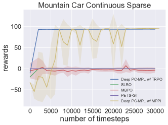
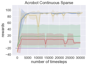
Figure 6: Performance comparison between our two practical implementations.

C.2 Computation Efficiency of PC-MLP

In this section, we investigate the wall-clock running time of Deep PC-MLP comparing with other baselines. We test on the running time of each algorithm on the MountainCar environment. We summarize the wall-clock running time in table 3. We see that our practical implementation can run as fast as other baselines. Taking the computation of exploration bonus into consideration, the results show that our algorithm is indeed computationally efficient.

	Time
PC-MLP	148m43s
PETS-GT	132m50s
MBPO	153m30s

Table 3: Wall-clock running time comparison

Appendix D Experimental Details

D.1 MPPI Pseudocode

Here we present the pseudocode for MPPI in Alg. 3:

0:  Learned dynamics $\hat{P}$, reward $r$, number of samples $K$, shooting horizon $H$, noise convariance $\Sigma$, temperature $\lambda$, initial state $s_{0}$

1:  if First time planning then

2:     Initialize $\{a_{0},a_{1},\dots,a_{T-1}\}$

3:  end if

4:  for $k=1,\dots,K$ do

5:     Sample $\mathcal{E}^{k}=\{\varepsilon_{0}^{k},\varepsilon_{1}^{k},\dots,\varepsilon_{T-1}^{k}\}$

6:     for $t=1,\dots,T$ do

7:        $S(\mathcal{E}^{k})\mathrel{+}=-r(s_{t-1},a_{t-1}+\varepsilon^{k}_{t-1})+\lambda a_{t-1}^{T}\Sigma^{-1}\epsilon_{t-1}^{k}$

8:        $s_{t}=\hat{P}(s_{t-1},a_{t-1}+\varepsilon^{k}_{t-1})$

9:     end for

10:     $\beta=\min_{k}S(\mathcal{E}^{k})$

11:     $\eta=\sum_{k=0}^{K-1}\exp{\left(-\frac{1}{\lambda}\left(S(\mathcal{E}^{k})-\beta\right)\right)}$

12:     for $k=1,\dots,K$ do

13:        $w(\mathcal{E}^{k})=\frac{1}{\eta}\exp{\left(-\frac{1}{\lambda}\left(S(\mathcal{E}^{k})-\beta\right)\right)}$

14:     end for

15:     for $t=1,\dots,T$ do

16:        $a_{t}\mathrel{+}=\sum_{k=1}^{K}w(\mathcal{E}^{k})\epsilon^{k}_{t}$

17:     end for

18:  end for

19:  $a=a_{0}$

20:  for $t=1,\dots,T-1$ do

21:     $a_{t-1}=a_{t}$

22:  end for

23:  Initialize $a_{T-1}$

Algorithm 3 MPPI

D.2 Hyperparameters of Deep PC-MLP

D.2.1 MountainCar and Acrobot

We provide the hyperparameters we considered and finally adopted for MountainCar and Acrobot environments in Table 4 (using TRPO as the planner) and Table 5 (using MPPI as the planner).

	Value Considered	Final Value
Model Learning Rate	{1e-3, 5e-3, 1e-4}	1e-3
Dynamics Model Hidden Layer Size	{[500,500]}	[500,500]
Policy Learning Rate	{3e-4}	3e-4
Policy Hidden Layer Size	{[32,32]}	[32,32]
Number of Model Updates	{100}	100
Number of Policy Updates	{40}	40
Number of Iterations	{30,60}	15
Multistep Loss L	{2}	2
Sample Size per Iteration (K)	{1000,2000,3000}	2000
Covariance Regulerazation Coefficient ($\lambda$)	{1,0.1,0.01,0.001}	0.01
Replay Buffer Size	{30000}	30000
Bonus Scale ($C$)	{1,2,5}	5

Table 4: Hyperparameter for MountainCarContinuous environment using TRPO as planner.

	Value Considered	Final Value
Learning Rate	{1e-3, 5e-3, 1e-4}	5e-3
Hidden Layer Size	{64}	64
Number of Iterations	{30,60}	30
Sample Size per Iteration (K)	{1000,2000,3000}	1000
Covariance Regulerazation Coefficient ($\lambda$)	{1,0.1,0.01,0.001}	0.01
Replay Buffer Size	{10000}	10000
Bonus Scale ($C$)	{1,2}	1
Dimention of RFF Feature ($|\phi|$)	{10,15,20,30}	20
MPPI Sampling Size (K)	{15,100,200,300}	200
MPPI Shooting Horizon (H)	{15,30,45,60}	30
MPPI Temperature ($\lambda$)	{1,0.2,0.1,0.001}	0.2
MPPI Noise Covariance ($\Sigma$)	{0.2,0.3,0.5,1}$I$	0.3$I$

Table 5: Hyperparameter for MountainCarContinuous environment using MPPI as planner.

D.2.2 Hand Egg and Dense Reward Environments

We provide the hyperparameters we considered and finally adopted for Hand Egg and dense reward environments in Table 6.

	Value Considered	Final Value
Model Learning Rate	{1e-3, 5e-3, 1e-4}	1e-3
Dynamics Model Hidden Layer Size	{[500,500]}	[500,500]
Policy Learning Rate	{3e-4}	3e-4
Policy Hidden Layer Size	{[32,32]}	[32,32]
Number of Model Updates	{100}	100
Number of Policy Updates	{40}	40
Number of Iterations	{200,100,50}	50
Multistep Loss L	{2}	2
Sample Size per Iteration (K)	{1000,2000,4000}	4000
Covariance Regulerazation Coefficient ($\lambda$)	{1,0.1,0.01,0.001}	0.01
Replay Buffer Size	{100000}	100000
Bonus Scale ($C$)	{0.1,1}	0.1

Table 6: Hyperparameter for HandEgg and dense reward environment.

References

• Abbasi-Yadkori & Szepesvári (2011) Abbasi-Yadkori, Y. and Szepesvári, C. Regret bounds for the adaptive control of linear quadratic systems. In Conference on Learning Theory, pp.  1–26, 2011.
• Agarwal et al. (2020a) Agarwal, A., Henaff, M., Kakade, S., and Sun, W. Pc-pg: Policy cover directed exploration for provable policy gradient learning. arXiv preprint arXiv:2007.08459, 2020a.
• Agarwal et al. (2020b) Agarwal, A., Kakade, S., Krishnamurthy, A., and Sun, W. Flambe: Structural complexity and representation learning of low rank mdps. arXiv preprint arXiv:2006.10814, 2020b.
• Ayoub et al. (2020) Ayoub, A., Jia, Z., Szepesvari, C., Wang, M., and Yang, L. F. Model-based reinforcement learning with value-targeted regression. arXiv preprint arXiv:2006.01107, 2020.
• Bansal et al. (2017) Bansal, S., Calandra, R., Xiao, T., Levine, S., and Tomiin, C. J. Goal-driven dynamics learning via bayesian optimization. In 2017 IEEE 56th Annual Conference on Decision and Control (CDC), pp.  5168–5173. IEEE, 2017.
• Botev et al. (2013) Botev, Z. I., Kroese, D. P., Rubinstein, R. Y., and L’Ecuyer, P. The cross-entropy method for optimization. In Handbook of statistics, volume 31, pp.  35–59. Elsevier, 2013.
• Brockman et al. (2016) Brockman, G., Cheung, V., Pettersson, L., Schneider, J., Schulman, J., Tang, J., and Zaremba, W. OpenAI gym. arXiv preprint arXiv:1606.01540, 2016.
• Burda et al. (2019) Burda, Y., Edwards, H., Storkey, A., and Klimov, O. Exploration by random network distillation. In International Conference on Learning Representations, 2019. URL https://openreview.net/forum?id=H1lJJnR5Ym.
• Chua et al. (2018) Chua, K., Calandra, R., McAllister, R., and Levine, S. Deep reinforcement learning in a handful of trials using probabilistic dynamics models. In Advances in Neural Information Processing Systems, pp. 4754–4765, 2018.
• Cohen et al. (2019) Cohen, A., Koren, T., and Mansour, Y. Learning linear-quadratic regulators efficiently with only sqrtT regret. In International Conference on Machine Learning, pp. 1300–1309, 2019.
• Dani et al. (2008) Dani, V., Hayes, T. P., and Kakade, S. M. Stochastic linear optimization under bandit feedback. In COLT, pp.  355–366, 2008.
• Dean et al. (2018) Dean, S., Mania, H., Matni, N., Recht, B., and Tu, S. Regret bounds for robust adaptive control of the linear quadratic regulator. In Advances in Neural Information Processing Systems, pp. 4188–4197, 2018.
• Deisenroth & Rasmussen (2011) Deisenroth, M. and Rasmussen, C. E. PILCO: A model-based and data-efficient approach to policy search. In International Conference on Machine Learning, pp. 465–472, 2011.
• Devroye et al. (2018) Devroye, L., Mehrabian, A., and Reddad, T. The total variation distance between high-dimensional gaussians. arXiv preprint arXiv:1810.08693, 2018.
• Fisac et al. (2018) Fisac, J. F., Akametalu, A. K., Zeilinger, M. N., Kaynama, S., Gillula, J., and Tomlin, C. J. A general safety framework for learning-based control in uncertain robotic systems. IEEE Transactions on Automatic Control, 64(7):2737–2752, 2018.
• Geramifard et al. (2015) Geramifard, A., Dann, C., Klein, R. H., Dabney, W., and How, J. P. Rlpy: a value-function-based reinforcement learning framework for education and research. J. Mach. Learn. Res., 16(1):1573–1578, 2015.
• Haarnoja et al. (2018) Haarnoja, T., Zhou, A., Abbeel, P., and Levine, S. Soft actor-critic: Off-policy maximum entropy deep reinforcement learning with a stochastic actor. In International Conference on Machine Learning, pp. 1861–1870. PMLR, 2018.
• Janner et al. (2019) Janner, M., Fu, J., Zhang, M., and Levine, S. When to trust your model: Model-based policy optimization. arXiv preprint arXiv:1906.08253, 2019.
• Jin et al. (2019) Jin, C., Yang, Z., Wang, Z., and Jordan, M. I. Provably efficient reinforcement learning with linear function approximation. arXiv preprint arXiv:1907.05388, 2019.
• Kaiser et al. (2019) Kaiser, L., Babaeizadeh, M., Milos, P., Osinski, B., Campbell, R. H., Czechowski, K., Erhan, D., Finn, C., Kozakowski, P., Levine, S., et al. Model-based reinforcement learning for atari. arXiv preprint arXiv:1903.00374, 2019.
• Kakade et al. (2020) Kakade, S., Krishnamurthy, A., Lowrey, K., Ohnishi, M., and Sun, W. Information theoretic regret bounds for online nonlinear control. arXiv preprint arXiv:2006.12466, 2020.
• Karaman & Frazzoli (2011) Karaman, S. and Frazzoli, E. Sampling-based algorithms for optimal motion planning. The international journal of robotics research, 30(7):846–894, 2011.
• Ko et al. (2007) Ko, J., Klein, D. J., Fox, D., and Haehnel, D. Gaussian processes and reinforcement learning for identification and control of an autonomous blimp. In Proceedings 2007 ieee international conference on robotics and automation, pp.  742–747. IEEE, 2007.
• Kurutach et al. (2018) Kurutach, T., Clavera, I., Duan, Y., Tamar, A., and Abbeel, P. Model-ensemble trust-region policy optimization. arXiv preprint arXiv:1802.10592, 2018.
• Levine & Abbeel (2014) Levine, S. and Abbeel, P. Learning neural network policies with guided policy search under unknown dynamics. In Advances in Neural Information Processing Systems, pp. 1071–1079, 2014.
• Lu & Van Roy (2019) Lu, X. and Van Roy, B. Information-theoretic confidence bounds for reinforcement learning. In Advances in Neural Information Processing Systems, pp. 2458–2466, 2019.
• Luo et al. (2018) Luo, Y., Xu, H., Li, Y., Tian, Y., Darrell, T., and Ma, T. Algorithmic framework for model-based deep reinforcement learning with theoretical guarantees. arXiv preprint arXiv:1807.03858, 2018.
• Mania et al. (2019) Mania, H., Tu, S., and Recht, B. Certainty equivalent control of LQR is efficient. arXiv preprint arXiv:1902.07826, 2019.
• Mania et al. (2020) Mania, H., Jordan, M. I., and Recht, B. Active learning for nonlinear system identification with guarantees. arXiv preprint arXiv:2006.10277, 2020.
• Modi et al. (2020) Modi, A., Jiang, N., Tewari, A., and Singh, S. Sample complexity of reinforcement learning using linearly combined model ensembles. In International Conference on Artificial Intelligence and Statistics, pp.  2010–2020, 2020.
• Moore (1990) Moore, A. W. Efficient memory-based learning for robot control. Technical report, 1990.
• Munos (2014) Munos, R. From bandits to monte-carlo tree search: The optimistic principle applied to optimization and planning. 2014.
• Nagabandi et al. (2018) Nagabandi, A., Kahn, G., Fearing, R. S., and Levine, S. Neural network dynamics for model-based deep reinforcement learning with model-free fine-tuning. In IEEE International Conference on Robotics and Automation, pp.  7559–7566, 2018.
• Osband & Van Roy (2014) Osband, I. and Van Roy, B. Model-based reinforcement learning and the Eluder dimension. In Advances in Neural Information Processing Systems, pp. 1466–1474, 2014.
• Plappert et al. (2018) Plappert, M., Andrychowicz, M., Ray, A., McGrew, B., Baker, B., Powell, G., Schneider, J., Tobin, J., Chociej, M., Welinder, P., et al. Multi-goal reinforcement learning: Challenging robotics environments and request for research. arXiv preprint arXiv:1802.09464, 2018.
• Rahimi & Recht (2008) Rahimi, A. and Recht, B. Random features for large-scale kernel machines. In Advances in neural information processing systems, pp. 1177–1184, 2008.
• Rajeswaran et al. (2020) Rajeswaran, A., Mordatch, I., and Kumar, V. A game theoretic framework for model based reinforcement learning. In International Conference on Machine Learning, pp. 7953–7963. PMLR, 2020.
• Ratliff et al. (2009) Ratliff, N., Zucker, M., Bagnell, J. A., and Srinivasa, S. Chomp: Gradient optimization techniques for efficient motion planning. In 2009 IEEE International Conference on Robotics and Automation, pp.  489–494. IEEE, 2009.
• Ross & Bagnell (2012) Ross, S. and Bagnell, J. A. Agnostic system identification for model-based reinforcement learning. arXiv preprint arXiv:1203.1007, 2012.
• Schrittwieser et al. (2019) Schrittwieser, J., Antonoglou, I., Hubert, T., Simonyan, K., Sifre, L., Schmitt, S., Guez, A., Lockhart, E., Hassabis, D., Graepel, T., et al. Mastering atari, go, chess and shogi by planning with a learned model. arXiv preprint arXiv:1911.08265, 2019.
• Schulman et al. (2015) Schulman, J., Levine, S., Abbeel, P., Jordan, M., and Moritz, P. Trust region policy optimization. In International Conference on Machine Learning, pp. 1889–1897, 2015.
• Simchowitz & Foster (2020) Simchowitz, M. and Foster, D. J. Naive exploration is optimal for online LQR. arXiv preprint arXiv:2001.09576, 2020.
• Sun et al. (2016) Sun, W., van den Berg, J., and Alterovitz, R. Stochastic extended lqr for optimization-based motion planning under uncertainty. IEEE Transactions on Automation Science and Engineering, 13(2):437–447, 2016.
• Sun et al. (2018) Sun, W., Gordon, G. J., Boots, B., and Bagnell, J. Dual policy iteration. In Advances in Neural Information Processing Systems, pp. 7059–7069, 2018.
• Sun et al. (2019) Sun, W., Jiang, N., Krishnamurthy, A., Agarwal, A., and Langford, J. Model-based RL in contextual decision processes: PAC bounds and exponential improvements over model-free approaches. In Conference on Learning Theory, pp.  1–36, 2019.
• Sutton (1996) Sutton, R. S. Generalization in reinforcement learning: Successful examples using sparse coarse coding. Advances in neural information processing systems, pp. 1038–1044, 1996.
• Todorov & Li (2005) Todorov, E. and Li, W. A generalized iterative lqg method for locally-optimal feedback control of constrained nonlinear stochastic systems. In Proceedings of the 2005, American Control Conference, 2005., pp.  300–306. IEEE, 2005.
• Todorov et al. (2012) Todorov, E., Erez, T., and Tassa, Y. Mujoco: A physics engine for model-based control. In 2012 IEEE/RSJ International Conference on Intelligent Robots and Systems, pp.  5026–5033. IEEE, 2012.
• Trott et al. (2019) Trott, A., Zheng, S., Xiong, C., and Socher, R. Keeping your distance: Solving sparse reward tasks using self-balancing shaped rewards. Advances in Neural Information Processing Systems, 32:10376–10386, 2019.
• Umlauft et al. (2018) Umlauft, J., Pöhler, L., and Hirche, S. An uncertainty-based control lyapunov approach for control-affine systems modeled by gaussian process. IEEE Control Systems Letters, 2(3):483–488, 2018.
• Wang et al. (2019) Wang, T., Bao, X., Clavera, I., Hoang, J., Wen, Y., Langlois, E., Zhang, S., Zhang, G., Abbeel, P., and Ba, J. Benchmarking model-based reinforcement learning. arXiv preprint arXiv:1907.02057, 2019.
• Williams et al. (2017a) Williams, G., Aldrich, A., and Theodorou, E. A. Model predictive path integral control: From theory to parallel computation. Journal of Guidance, Control, and Dynamics, 40(2):344–357, 2017a.
• Williams et al. (2017b) Williams, G., Wagener, N., Goldfain, B., Drews, P., Rehg, J. M., Boots, B., and Theodorou, E. A. Information theoretic mpc for model-based reinforcement learning. In 2017 IEEE International Conference on Robotics and Automation (ICRA), pp.  1714–1721. IEEE, 2017b.
• Yang & Wang (2019) Yang, L. F. and Wang, M. Reinforcement leaning in feature space: Matrix bandit, kernels, and regret bound. arXiv preprint arXiv:1905.10389, 2019.
• Zhou et al. (2020) Zhou, D., He, J., and Gu, Q. Provably efficient reinforcement learning for discounted mdps with feature mapping. arXiv preprint arXiv:2006.13165, 2020.