Slow diffusion is necessary to explain the $\gamma$-ray pulsar halos

Abstract

It was suggested that the $\gamma$-ray halo around Geminga might not be interpreted by slow-diffusion. If the ballistic regime of electron/positron propagation is considered, the Geminga halo may be explained even with a large diffusion coefficient. In this work, we examine this effect by taking the generalized Jüttner propagator as the approximate relativistic Green’s function for diffusion and find that the morphology of the Geminga halo can be marginally fitted in the fast-diffusion scenario. However, the recently discovered $\gamma$-ray halo around PSR J0622$+$3749 at LHAASO cannot be explained by the same effect and slow diffusion is the only solution. Furthermore, both the two pulsar halos require a conversion efficiency from the pulsar spin-down energy to the high energy electrons/positrons much larger than 100%, if they are interpreted by this ballistic transport effect. Therefore, we conclude that slow diffusion is necessary to account for the $\gamma$-ray halos around pulsars.

1 Introduction

It has been predicted that a middle-aged pulsar should be surrounded by a $\gamma$-ray halo (Linden et al., 2017). The $\gamma$-ray halo is generated by the high-energy electrons and positrons, accelerated by the central pulsar wind nebula (PWN), scattering with the background photons when they are injected and propagate in the interstellar medium. The $\gamma$-ray halos around Geminga and Monogem were first detected by the HAWC Collaboration (Abeysekara et al., 2017). The most intriguing feature of the halos is that the diffusion coefficients indicated by the $\gamma$-ray profiles are much smaller than the average value in the Galaxy derived by the B/C data.

Recently, a paper by Recchia et al. (2021) points out another plausible scenario, in which the pulsar halo may be explained without a slow-diffusion environment. It is well known that the non-relativistic diffusion equation has the superluminal problem. For the relativistic particles injected within the time $t_{\rm crit}\equiv 3D/c^{2}$, the typical diffusion distance $\lambda\sim\sqrt{Dt}$ is greater than $ct$, where $D$ is the diffusion coefficient and $c$ is the light speed. For $t\ll t_{\rm crit}$, the particles should propagate ballistically rather than diffusively. They found that the ballistic propagation and the transition to the diffusion regime may explain the Geminga halo even assuming a typical diffusion coefficient in the Galaxy.

The superluminal problem in non-relativistic diffusion equation has been studied by Aloisio et al. (2009). It is found that the generalized Jüttner propagator can be taken as the approximate relativistic Green’s function for diffusion although a full relativistic diffusion equation has not been developed (Aloisio et al., 2009). The method used by Recchia et al. (2021) can be considered as an approximate form of the Jüttner propagator to describe the ballistic and quasi-ballistic propagation.

In this work, we examine the effect of relativistic diffusion on the interpretation of the $\gamma$-ray pulsar halos. We adopt the generalized Jüttner propagator as the relativistic Green’s function for the diffusion equation. Besides the Geminga halo that has been paid great attention, we also test another newly discovered $\gamma$-ray halo around PSR J0622$+$3749 by LHAASO-KM2A (Aharonian et al., 2021), which is very likely an analog of the Geminga halo.

We find that if the effect of ballistic propagation is taken into account the profile of the $\gamma$-ray halo around Geminga can be roughly fitted and the result by Recchia et al. (2021) is repeated. However, the same effect cannot account for the $\gamma$-ray halo profile around PSR J0622$+$3749 and slow diffusion is still necessary in this case. Furthermore, for the large diffusion coefficients the conversion efficiencies from pulsar spin-down energy to the high energy electrons are much greater than 100% for both the two halos.

In the next section, we will present our calculation and the results. Then we give the conclusion.

2 Calculation and Results

Pulsar halos are generated by electrons escaping from the PWNe and wandering in the ISM. Thus, solving the electron propagation equation in the ISM is the core of calculating the halo morphology. The electron propagation can be expressed by the diffusion-cooling equation:

$$\frac{\partial N(E,\boldsymbol{r},t)}{\partial t}=D(E)\Delta N(E,\boldsymbol{r},t)+\frac{\partial[b(E)N(E,\boldsymbol{r},t)]}{\partial E}+Q(E,\boldsymbol{r},t)\ ,$$ (1)

where $E$ is the electron energy, and $N$ is the electron number density. The diffusion coefficient is taken as $D(E)=D_{0}(E/1~{}{\rm GeV})^{\delta}$, where we assume $\delta=1/3$ following the Komolgorov’s theory.

The energy-loss rate is defined by $b(E)=-{\rm d}E/{\rm d}t$ and can be expressed by $b(E)=b_{0}E^{2}$. ICS and synchrotron radiation dominate the energy losses of high-energy electrons. Considering the Klein-Nishina effect in ICS, $b_{0}$ should be energy dependent. We adopt the parameterization given by Fang et al. (2021a) to precisely calculate the ICS component. The seed photon fields for ICS are taken from Abeysekara et al. (2017) and Fang et al. (2021b) for Geminga and LHAASO J0621$+$3755, respectively. We take the magnetic field to be 3 ${\rm\mu}$G for both the cases to get the synchrotron component.

The source function is taken as

$$Q(E,\boldsymbol{r},t)=\left\{\begin{aligned} &q(E)\ \delta(\boldsymbol{r}-\boldsymbol{r}_{s})\ (1+t/t_{\rm sd})^{-2}/(1+t_{s}/t_{\rm sd})^{-2}\ ,&t\geq 0\\ &0\ ,&t<0\end{aligned}\right.\ ,$$ (2)

where $q(E)$ is the electron injection spectrum at the current time, $\boldsymbol{r}_{s}$ is the position of the pulsar, $t_{s}$ is the pulsar age, and $t_{\rm sd}$ is the typical spin-down time scale of pulsar, which is set to be 10 kyr.

We assume the injection spectrum to be a power-law form with an exponential cutoff:

$$q(E)=q_{0}(E/{\rm 1~{}GeV})^{-p}\ {\rm exp}[-(E/E_{c})^{2}]\ ,$$ (3)

where the values of $p$ and $E_{c}$ are listed in Table. 1, and the normalization $q_{0}$ can be determined by the relation

$$\int q(E)E{\rm d}E=\eta L\ ,$$ (4)

where $L$ is the current spin-down luminosity of the pulsar and $\eta$ is the conversion efficiency from the spin-down energy to the electron energy. For the Geminga halo, the spectral parameters are determined by a rough fit to a preliminary $\gamma$-ray spectrum of HAWC (Zhou, 2019). For LHAASO J0621$+$3755, we adopt the best-fit spectral parameters to the LHAASO-KM2A spectrum (Aharonian et al., 2021; Fang et al., 2021b).

We can obtain the solution of Eq. (1) with the Green’s function method:

$$N(E,\boldsymbol{r},t)=\int_{\mathbb{R}^{3}}{\rm d}^{3}\boldsymbol{r}_{0}\int_{-\infty}^{t}{\rm d}t_{0}\int_{-\infty}^{+\infty}{\rm d}E_{0}\,G(E,\boldsymbol{r},t;E_{0},\boldsymbol{r}_{0},t_{0})\,Q(E_{0},\boldsymbol{r}_{0},t_{0})\ .$$ (5)

In the normal diffusion model, the Green’s function is expressed as

$$G(E,\boldsymbol{r},t;E_{0},\boldsymbol{r}_{0},t_{0})=\frac{1}{b(E)(\uppi\lambda^{2})^{3/2}}\ {\rm exp}\left[-\frac{(\boldsymbol{r}-\boldsymbol{r}_{0})^{2}}{\lambda^{2}}\right]\ \delta(t-t_{0}-\tau)\ H(\tau)\ ,$$ (6)

where

$$\lambda=2\sqrt{\int_{E}^{E_{0}}\ \frac{D(E^{\prime})}{b(E^{\prime})}\ {\rm d}E^{\prime}}\ ,\quad\tau=\int_{E}^{E_{0}}\frac{{\rm d}E^{\prime}}{b(E^{\prime})}\ ,$$ (7)

and $H$ is the Heaviside step function.

In order to eliminate superluminal motion, we need to find the relativistic correction of Eq. (1). Unfortunately, many efforts over decades have not been successful so far. To evade this difficulty, Dunkel et al. (2007a) noticed that the propagator

$$P(E,r,t)=\frac{1}{(\uppi\lambda^{2})^{3/2}}{\rm exp}\left(-\frac{r^{2}}{\lambda^{2}}\right)$$ (8)

has the same form with the Maxwell-Boltzmann speed distribution of particles with mass $m$ in thermal equilibrium gas with temperature $T$:

$$f_{\rm{M-B}}(\boldsymbol{v})=\left(\frac{m}{2\uppi kT}\right)^{3/2}\ {\rm exp}\left(-\frac{mv^{2}}{2kT}\right)\ ,$$ (9)

if we make the replacements $v\rightarrow x$ and $2kT/m\rightarrow\lambda^{2}$. Jüttner (1911) derived the Maxwell-Jüttner distribution which describes the speeds of relativistic particles in thermal equilibrium gas:

$$f_{\rm{M-J}}(\boldsymbol{p})=\frac{1}{4\uppi(mc)^{3}}\ \frac{\mu}{K_{2}(\mu)}\ {\rm exp}(-\gamma\mu)\ ,$$ (10)

where $\boldsymbol{p}=\gamma m\boldsymbol{v}$ represents the momentum, $\gamma=1/\sqrt{1-v^{2}/c^{2}}$ represents the Lorentz factor, $\mu=mc^{2}/kT$, and $K_{\nu}$ is the $\nu$-order modified Bessel function of the second kind. From the relationship $4\uppi v^{2}f_{v}(\boldsymbol{v}){\rm d}v=4\uppi p^{2}f_{p}(\boldsymbol{p}){\rm d}p$, we derive

$$f_{\rm{M-J}}(\boldsymbol{v})=\frac{\gamma^{5}}{4\uppi c^{3}}\ \frac{\mu}{K_{2}(\mu)}\ {\rm exp}(-\gamma\mu)\ .$$ (11)

However, the standard form Eq. (11) might not represent the correct relativistic equilibrium distribution (Dunkel et al., 2007b). A modification

$$f_{\rm{M-J}}(\boldsymbol{v})=\frac{\gamma^{4}}{4\uppi c^{3}}\ \frac{\mu}{K_{1}(\mu)}\ {\rm exp}(-\gamma\mu)\$$ (12)

is most frequently suggested.

It reminds us to take Eq. (12) with the same replacements $v\rightarrow r$, $2kT/m\rightarrow\lambda^{2}$ and $c\rightarrow ct$ as the propagator in the Green’s function, called the generalized Jüttner propagator (Aloisio et al., 2009):

$$P_{\rm rela}(E,r,t)=\frac{1}{4\uppi(ct)^{3}}\ \frac{H[1-\xi(r,t)]}{[1-\xi^{2}(r,t)]^{2}}\ \frac{\kappa(E,t)}{K_{1}[\kappa(E,t)]}\ {\rm exp}\left[-\frac{\kappa(E,t)}{\sqrt{1-\xi^{2}(r,t)}}\right]\ ,$$ (13)

where $\xi(r,t)=r/ct$ and $\kappa(E,t)=2(ct/\lambda)^{2}$. The Heaviside step function $H$ is used to ensure that $P_{\rm rela}$ vanishes when $r>ct$. In the extreme case of $\kappa\ll 1$ or $\kappa\gg 1$, the propagator will transit to ballistic or diffusive propagator separately (see Appendix A). In this way we derive the Green’s function with relativistic correction:

$$G_{\rm rela}(E,\boldsymbol{r},t;E_{0},\boldsymbol{r}_{0},t_{0})=\frac{1}{4\uppi[c(t-t_{0})]^{3}b(E)}\ \frac{H(1-\xi)}{(1-\xi^{2})^{2}}\ \frac{\kappa}{K_{1}(\kappa)}\ {\rm exp}\left(-\frac{\kappa}{\sqrt{1-\xi^{2}}}\right)\ \delta(t-t_{0}-\tau)\ H(\tau)\ ,$$ (14)

where $\xi=(\boldsymbol{r}-\boldsymbol{r}_{0})/c(t-t_{0})$ and $\kappa=2[c(t-t_{0})/\lambda]^{2}$.

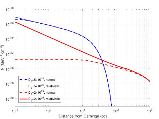
Figure 1: Electron number densities as functions of the distance from Geminga for the slow-diffusion ($D_{0}=5\times 10^{25}$ cm² s^-1) and fast-diffusion ($D_{0}=2\times 10^{29}$ cm² s^-1) scenarios. Both the relativistic and non-relativistic diffusion models are presented. The conversion efficiency is set as 100% for all the cases in this figure.

In Fig. 1, we draw $N$ as functions of the distance from Geminga to show the effect of relativistic correction. The electron energy is 100 TeV, which is roughly the parent electron energy of the TeV pulsar halos. The conversion efficiency is set as 100% for all the cases. As expected, there is little difference between the standard and relativistic diffusion models in the slow-diffusion scenario. When the diffusion coefficient is significantly larger, the relativistic correction is crucial. The newly injected electrons are still in the ballistic regime and cannot flee far away from the source with superluminal velocities, leading to a more constrictive distribution than that of the non-relativistic case. However, although the fast-diffusion scenario can also predict a steep electron distribution near the source after the relativistic correction, the absolute $N$ is about an order of magnitude smaller than that of the slow-diffusion scenario. It means that a significantly larger conversion efficiency is required for the former to explain a same observation.

Due to the anisotropy of inverse Compton scattering (ICS) processes of the quasi-ballistic electrons within the vicinity of source, it is necessary to consider the velocity angular distribution of the electrons in the small-angle region with the following form (Prosekin et al., 2015), the details of which are discussed in Appendix B:

$$M(x,\alpha)=\frac{1}{Z(x)}\ \mathrm{exp}[-\frac{3(1-\alpha)}{x}]\ ,$$ (15)

where $x(r,E)=rc/D(E)$, $Z(x)=\frac{x}{3}[1-\mathrm{exp}(-\frac{6}{x})]$ is the normalization coefficient, and $\alpha$ is the cosine of the angle $\phi$ between the radial direction and the line of sight.

We integrate $2NM$ over the line of sight from the Earth to an angle of $\theta$ observed away from the pulsar to get the apparent electron surface density and then obtain the $\gamma$-ray surface brightness profile (SBP) with the standard calculation of ICS (Blumenthal & Gould, 1970). For the case of LHAASO J0621$+$3755, the point-spread function (PSF) must be convoluted with our calculation results:

$$\frac{{\rm d}\Phi}{{\rm d}\Omega}^{\ast}(\theta_{x},\theta_{y})=(\frac{{\rm d}\Phi}{{\rm d}\Omega}\ast{\rm PSF})\ (\theta_{x},\theta_{y})=\iint_{\mathbb{R}^{2}}\frac{{\rm d}\Phi}{{\rm d}\Omega}(\delta_{x},\delta_{y})\ {\rm PSF}(\theta_{x}-\delta_{x},\theta_{y}-\delta_{y})\ {\rm d}\delta_{x}\ {\rm d}\delta_{y}\ ,$$ (16)

where ${\rm d}\Phi/{\rm d}\Omega$ is the flux per unit solid angle at the point with coordinates $(\theta_{x},\theta_{y})$ in the image plane predicted by our model, the star mark ${\ast}$ represents the convolution results. We emphasize that the PSF is a 2-dimentional (2D) Gaussian function as

$${\rm PSF}(\theta_{x},\theta_{y})=\frac{1}{2\uppi\sigma^{2}}\ {\rm exp}\left(-\frac{\theta_{x}^{2}+\theta_{y}^{2}}{2\sigma^{2}}\right)\ ,$$ (17)

where $\sigma=0.45^{\circ}$ (Aharonian et al., 2021). For each angular distance $\theta$, we take the average value of $({\rm d}\Phi/{\rm d}\Omega)^{\ast}$ to get the SBP:

$${\rm SBP}(\theta)=\frac{1}{2\uppi}\ \int_{0}^{2\uppi}\frac{{\rm d}\Phi}{{\rm d}\Omega}^{\ast}(\theta{\rm cos}\varphi,\theta{\rm sin}\varphi)\ {\rm d}\varphi\ .$$ (18)

We vary the diffusion coefficient $D_{0}$ from $10^{25}$ to $10^{30}$ cm² s^-1 and take the energy conversion efficiency $\eta$ as the free parameter to fit the HAWC data for Geminga and the LHASSO-KM2A data for LHAASO J0621$+$3755, using the least-$\chi^{2}$ method. Other determined parameters are summarized in Table. 1. The details about the parameters $E_{c}$ and $p$ of the injection spectrum refer to Appendix C.

Table 1: Model parameters for Geminga and LHAASO J0621$+$3755.

	Geminga	J0621
$t_{s}~{}({\rm kyr})$	$342$	$208$
$r_{s}~{}({\rm pc})$	$250$	$1600$
$L~{}(\rm{erg~{}s^{-1}})~{}$	$~{}3.2\times 10^{34}~{}$	$~{}2.7\times 10^{34}$
$p$	$1.0$	$1.5$
$E_{c}~{}({\rm TeV})$	$133$	$265$

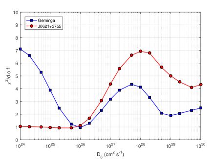
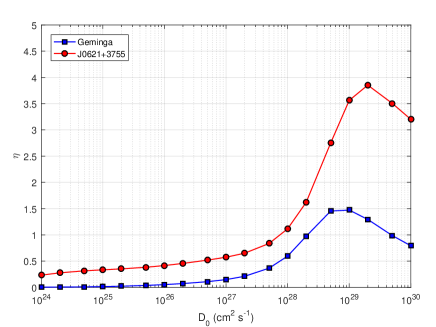
Figure 2: Left: The minimal $\chi^{2}$ of best fitting to the $\gamma$-ray halo profiles as function of diffusion coefficient at 1 GeV. Right: The efficiency of energy transfer from the pulsar spin-down energy to electron/positron pairs for different values of $D_{0}$.

We illustrate the fitting results in Fig. 2. It is clear that there are two minimal values of $\chi^{2}$ for the Geminga case. The solution of the slow-diffusion scenario with $D_{0}=1\times 10^{26}~{}\mathrm{cm^{2}~{}s^{-1}}~{}[D(100~{}\mathrm{TeV})=5\times 10^{27}~{}\mathrm{cm^{2}~{}s^{-1}}]$ gives very good fit to the data with $\chi^{2}/\rm{d.o.f.}\sim 1$. The fast-diffusion scenario with $D_{0}=1\times 10^{29}~{}\mathrm{cm^{2}~{}s^{-1}}~{}[D(100~{}\mathrm{TeV})=5\times 10^{30}~{}\mathrm{cm^{2}~{}s^{-1}}]$ gives a poorer fit with $\chi^{2}/\rm{d.o.f.}\sim 2$, which is in agreement with the result by Recchia et al. (2021). The best fitted fast diffusion coefficient is slightly larger than the Galactic typical value derived by the B/C data (Yuan et al., 2017). The required $\eta$ for the slow-diffusion scenario is $\sim 5\%$, while the fast-diffusion scenario needs a conversion efficiency of $\sim 150\%$, exceeding 100%.

There are also two local minimal $\chi^{2}$ for the case of LHAASO J0621$+$3755, corresponding to $D_{0}=5\times 10^{25}~{}\mathrm{cm^{2}~{}s^{-1}}~{}[D(100~{}\mathrm{TeV})=2\times 10^{27}~{}\mathrm{cm^{2}~{}s^{-1}}]$ and $D_{0}=5\times 10^{29}~{}\mathrm{cm^{2}~{}s^{-1}}~{}[D(100~{}\mathrm{TeV})=2\times 10^{31}~{}\mathrm{cm^{2}~{}s^{-1}}]$, respectively. However, only the slow-diffusion solution can fit the LHAASO-KM2A data. The minimal $\chi^{2}/\rm{d.o.f.}$ in the fast-diffusion regime is about 4, corresponding an exclusion with a confidence level of 99.996%. The problem of conversion efficiency is also serious for the fast-diffusion solution, as $\eta\sim 350\%$. This value may not be reasonable even considering the uncertainties of the pulsar spin-down luminosity and the required total electron energy.

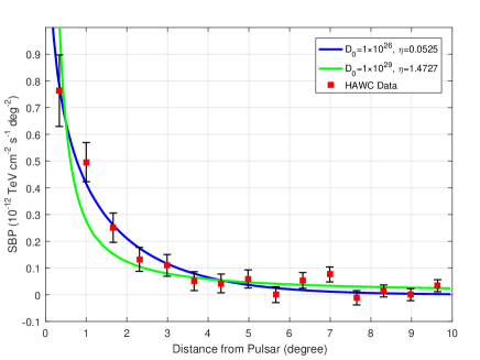
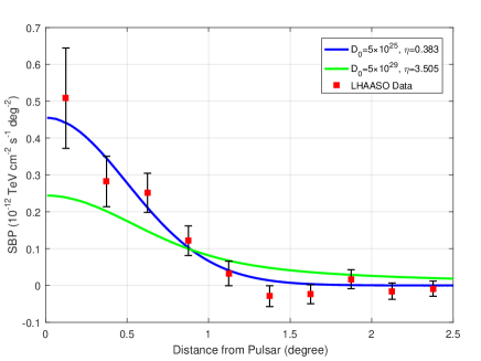
Figure 3: The $\gamma$-ray profiles of the Geminga halo (left) and LHAASO J0621$+$3755 (right) taking $D_{0}$ corresponding to the two local minimal $\chi^{2}$.

In Fig. 3, we show the theoretical SBPs corresponding to the two local minimal $\chi^{2}$ for both the Geminga halo and LHAASO J0621$+$3755. As already indicated by the $\chi^{2}$ test, the fast-diffusion scenario can roughly fit the measured SBP of the Geminga halo, while gives a very poor fit to that of LHAASO J0621$+$3755. The predicted SBP is systematically lower than the data within $\sim 1^{\circ}$ from the pulsar and higher outside.

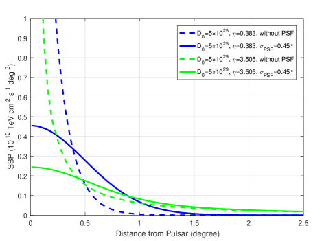
Figure 4: Comparison of the $\gamma$-ray profiles for LHAASO J0621$+$3755 before and after PSF convolution.

To understand the reason that the $\gamma$-ray profile of LHAASO J0621$+$3755 cannot be well fitted, we show the $\gamma$-ray profiles for LHAASO J0621$+$3755 with/without PSF convolution in solid/dashed lines in Fig. 4. For both slow-diffusion and fast-diffusion scenarios, $\eta$ is set to be the same value of SBP blurred by a 2D Gaussian function with a size of 0.45^∘ (in solid lines). The trends of the two dashed lines are similar to those of Geminga. In the case of fast diffusion, the green dashed line decreases more steeply in a small region around the pulsar than the blue dashed line. However, when the $\gamma$-ray profile is convolved with a large PSF, each flux point is affected by a broad range of the original profile. For example, the flux at $\theta=\sigma_{\rm PSF}=0.45^{\circ}$ of the original profile contributes to the flux at $\theta=0^{\circ}$ of the convolved profile. The original profile of the fast-diffusion case is significantly lower and flatter than the slow-diffusion case when $\theta>0.1^{\circ}$. Thus, even though the original profile of the fast-diffusion case is steeper in the most inner region, the convolved profile is lower and flatter as affected by the flux of large angular distances. Therefore, the green solid line becomes flatter after the PSF convolution and cannot fit the data.

Moreover, the fast-diffusion scenario is not equal to the pure ballistic propagation, but should be seen as a combination of the ballistic propagation for the latest injected electrons and the standard diffusion for early injected electrons. The ballistic component originates from the freshly-injected electrons with $t-t_{0}\ll t_{\rm crit}$, and the diffusive component originates from the electrons injected earlier with $t-t_{0}\gg t_{\rm crit}$. The pure ballistic component has a steep profile near the source and is a point-like source. The PSF convolved profile of this component should be similar to the PSF. However, the diffusive component is very extended in the fast diffusion scenario, and the PSF convolved profile is significantly broader than the PSF. Thus, the superposition of these two components don’t follow the PSF shape.

We illustrate this point in Fig. 5. We divide the profile of LHAASO J0621$+$3755 into two parts. One is generated by electrons injected in the most recent 100 years, which is almost a pure ballistic regime. The other is generated by electrons injected in the transitional (from pure ballistic to pure diffusion) and diffusive regimes. The left panel of Fig. 5 shows the profiles without the PSF convolution. The ballistic component shown in red solid line is very sharp and point-like, restricted to a small range around the source by the vertical black line, which represents the speed of light. The red dashed line dominates the flux at the outer region, consisting of a flat background contributed by the transitional and diffusive component. Therefore, the total profile can be seen as a superposition of a point-like source and a disk-like source. After the convolution with the PSF, the point-like component is significantly flattened and has a similar profile with the PSF, as shown in the right panel of Fig. 5. Meanwhile, the disk-like component is less affected by the convolution as it is much broader than the PSF. The total profile is the superposition of a PSF-like component and a dominant component with a much larger extension, which is not a PSF shape.

It can also be seen in Fig. 4 that the profile larger than $0.5^{\circ}$ is affected little by the convolution for the fast-diffusion case. If we force the inner fluxes to fit the data, the outer fluxes will be significantly higher than the data. Thus, the fast-diffusion model cannot fit the observation for the case of LHAASO J0621$+$3755.

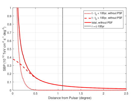
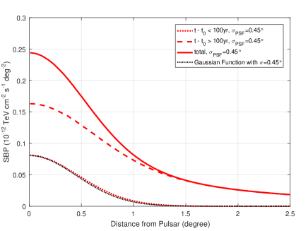
Figure 5: The two parts of the $\gamma$-ray profile of LHAASO J0621$+$3755 under the fast-diffusion scenario without (left) and with (right) the PSF convolution.

Our fitting result of LHAASO J0621$+$3755 is in conflict with that of Recchia et al. (2021), which finds that the goodness of fit for the fast-diffusion scenario is almost equal to the slow-diffusion scenario, and the efficiency of energy conversion is between 40% and 100%. The results are due to a wrong PSF convolution method that taking the PSF as an 1D Gaussian function in Recchia et al. (2021). Actually, the PSF is defined in the 2D image plane. Once the convolution method and the PSF form are replaced with the correct one, as shown in Eq. (16) and Eq. (17), the results for the fast-diffusion scenario become nearly the same as ours.

3 Conclusion

With a relativistic correction to the electron propagation equation, we examine if the morphologies of pulsar halos can be explained under the fast diffusion scenario, i.e., the typical diffusion coefficient in the Galaxy.

We find that the fast-diffusion scenario can give an acceptable fit to the $\gamma$-ray profile of the Geminga halo, which is in agreement with the result by Recchia et al. (2021). In relativistic diffusion, the propagation of newly injected electrons is ballistic, leading to a steep $\gamma$-ray profile near the source similar to the measurement. However, the required $\eta$ is 150%, which is too large. For LHAASO J0621$+$3755, the fast diffusion scenario cannot give reasonable fit to the profile. Therefore, the fast-diffusion scenario is strongly disfavored even with a relativistic correction.

In comparison, the slow-diffusion scenario can well fit the profiles with reasonable $\eta$ for both the two halos. Furthermore, the slow-diffusion assumption also matches the symmetry of the Geminga halo. If the diffusion coefficient is as large as the Galactic average, the mean free path of electrons at 100 TeV reaches tens of parsecs, which very likely corresponds to strong asymmetries of the halo (López-Coto & Giacinti, 2018). All these indicate that slow diffusion is still necessary to interpret pulsar halos.

Appendix A Discussion on the extreme cases of generalized Jüttner propagator

In the case of $\lambda\gg ct$, we have $\kappa\ll 1$ and

$$\frac{\kappa}{K_{1}(\kappa)}\ \approx\kappa^{2}\ .$$ (A1)

Substituting Eq.(A1) into Eq.(13), we have

$$P_{\rm rela}(E,r,t)\approx\frac{1}{4\uppi(ct)^{3}}\ \frac{H(1-\xi)}{(1-\xi^{2})^{2}}\ \kappa^{2}\ {\rm exp}\left(-\frac{\kappa}{\sqrt{1-\xi^{2}}}\right)\ =\frac{H(1-\xi)}{4\uppi(ct)^{3}}\ \frac{y{\rm d}y}{\xi{\rm d}\xi}\ {\rm exp}(-y)\ ,$$ (A2)

where $y=\kappa/\sqrt{1-\xi^{2}}$.

The ballistic propagator is written as

$$P_{\rm ball}(E,r,t)=\frac{1}{4\uppi c^{3}t^{2}}\ \delta(ct-r)\ .$$ (A3)

By evaluating the integral of Eq.(A3) multiplied by any function $q$ of $t$, we have

$$\int_{-\infty}^{+\infty}G_{\rm ball}(E,r,t)\ q(t)\ {\rm d}t=\frac{1}{4\uppi cr^{2}}\ q\left(\frac{r}{c}\right)\ .$$ (A4)

Applying the same operation to Eq.(A2), we obtain

$$\int_{-\infty}^{+\infty}P_{\rm rela}(E,r,t)\ q(t)\ {\rm d}t \approx\int_{\frac{r}{c}}^{+\infty}\frac{1}{4\uppi(ct)^{3}}\ \frac{y{\rm d}y}{\xi{\rm d}\xi}\ {\rm exp}(-y)\ q(t)\ {\rm d}t$$ (A5)

$$=\int_{0}^{+\infty}\frac{1}{4\uppi(ct)^{3}}\ \frac{r}{c\xi^{3}}\ y\ {\rm exp}(-y)\ q[t(y)]\ {\rm d}y$$

$$=\frac{1}{4\uppi cr^{2}}\ \int_{0}^{+\infty}y\ {\rm exp}(-y)\ q[t(y)]\ {\rm d}y\ ,$$

which coincides with Eq.(A4) because $\int_{0}^{+\infty}y\ {\rm exp}(-y)\ {\rm d}y=1$ and the approximation

$$t(y)=\frac{x}{c\sqrt{1-(\frac{\kappa}{y})^{2}}}\approx\frac{r}{c}\$$ (A6)

holds on the main part of integral interval.

In the case of $\lambda\ll ct$, we have $\kappa\gg 1$ and

$$\frac{\kappa}{K_{1}(\kappa)}\approx\sqrt{\frac{2}{\uppi}}\ \kappa^{3/2}\ {\rm exp}(\kappa)\ .$$ (A7)

At a distance $r\lesssim\lambda$ where the electron number density is non-ignorable, we obtain

$$\xi=\frac{r}{ct}\lesssim\frac{\lambda}{ct}\ll 1.$$ (A8)

Substituting Eq.(A7) and the first-order approximations $1/(1-\xi^{2})^{2}\approx 1$ and ${\rm exp}(-\kappa/\sqrt{1-\xi^{2}})\approx{\rm exp}[-\kappa(1+\xi^{2}/2)]$ into Eq.(13), we have

$$P_{\rm rela}(E,r,t)\approx\frac{1}{(ct)^{3}}\ \frac{1}{(1-\xi^{2})^{2}}\ \left(\frac{\kappa}{2\uppi}\right)^{3/2}\ {\rm exp}\left(-\frac{\kappa\xi^{2}}{2}\right)\ =\frac{1}{(\uppi\lambda^{2})^{3/2}}\ {\rm exp}\left(-\frac{r^{2}}{\lambda^{2}}\right)\ ,$$ (A9)

which coincides with Eq.(8), indicating that the propagator transits to the normal one.

Appendix B Discussion on the small-angle diffusion approximation

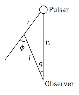
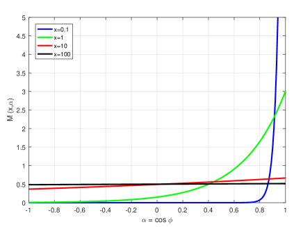
Figure 6: Left: A sketch map for the geometric parameters. Right: The small-angle diffusion approximation $M$ as a function of $\alpha$ for different $x$.

For the pure diffusion model, we directly integrate the electron number density $N$ over the line of sight to get the electron surface density

$$F_{\mathrm{diff}}(E,\theta)=\int^{\infty}_{0}N(E,l,\theta)\ \mathrm{d}l\ ,$$ (B1)

and then apply the standard ICS calculation, because the angular distribution of $\gamma$-ray is isotropic. But for the corrective model we use in this work, the angular distribution of $\gamma$-ray emitted by the quasi-ballistic electrons within the vicinity of source is anisotropic. Therefore, a small-angle correction is needed.

As a result of relativistic beaming effect, the angular distribution of $\gamma$-ray can be regarded as the velocity angular distribution of electrons. For the electrons with energy $E$ at the distance of $r$ from the source, let $\mathcal{M}(E,r,\Omega)\ \mathrm{d}\Omega$ represent the proportion that moves towards $\Omega(\phi,\varphi)$ within the solid angle $\mathrm{d}\Omega$. Here $\phi$ is the angle between the radial direction and the line of sight, as shown in the left panel of Fig. 6 together with other geometric parameters. From geometry, we derive $r(l,\theta)=\sqrt{r^{2}_{s}+l^{2}-2r_{s}l\mathrm{cos}\theta}$ and $\alpha(l,\theta)=\mathrm{cos}(\phi)=(r_{s}\mathrm{cos}\theta-l)/r$.

We introduce a dimensionless parameter $x(E,r)=rc/D(E)$. Because of the symmetry around the radial direction, the angle $\varphi$ is arbitrary and can be removed by integral:

$$\mathcal{M}(E,r,\Omega)=\mathcal{M}(x,\phi,\varphi)=\frac{1}{2\uppi}\ M(x,\phi).$$ (B2)

Taking the limit as $x\rightarrow\infty$, we get $\mathcal{M}_{\rm{diff}}=\frac{1}{4\uppi}$ and $M(\infty,\phi)=\frac{1}{2}$, because the case transits to pure diffusion scenario, as shown in the right panel of Fig. 6. Generally, $\mathcal{M}(E,r,\Omega)$ should be normalized by the solid angle $\Omega$. By $\mathrm{d}\Omega=\rm{sin}\phi\ \mathrm{d}\phi\mathrm{d}\varphi$, we derive

$$1 =\oiint\mathcal{M}(E,r,\Omega)\ \mathrm{d}\Omega=\oiint\mathcal{M}(x,\phi,\varphi)\ \rm{sin}\phi\ \mathrm{d}\phi\mathrm{d}\varphi$$ (B3)

$$=\int^{2\uppi}_{0}\ \mathrm{d}\varphi\ \int^{\uppi}_{0}\frac{1}{2\uppi}\ M(x,\phi)\ \mathrm{sin}\phi\ \rm{d}\phi$$

$$=\int^{-1}_{1}M(x,\phi)\ \mathrm{d}(-\mathrm{cos}\phi)=\int^{1}_{-1}M(x,\alpha)\ \mathrm{d}\alpha\ ,$$

where $\alpha=\mathrm{\phi}$. Prosekin et al. (2015) gives the form $M\sim\mathrm{exp}[-\frac{3(1-\alpha)}{x}]$, and the normalization function is

$$Z(x)=\int^{1}_{-1}\mathrm{exp}[-\frac{3(1-\alpha)}{x}]\ \mathrm{d}\alpha\ =\frac{x}{3}[1-\mathrm{exp}(-\frac{6}{x})]\ .$$ (B4)

This is exactly Eq. (15) we apply to our calculation. Then we get the apparent electron surface density:

$$F(E,\theta)=\int^{\infty}_{0}N(E,l,\theta)\ \frac{\mathcal{M}(E,r,\Omega)}{\mathcal{M}_{\rm{diff}}}\ \mathrm{d}l=\int^{\infty}_{0}2N(E,l,\theta)M(x,\alpha)\ \mathrm{d}l\ ,$$ (B5)

which is equivalent to the pure diffusion model and can be directly used in the standard ICS calculation.

Appendix C Discussion on the cutoff energy and the power-law index of the injection spectrum

Figure 7: The best-fit $\gamma$-ray spectrum to the HAWC data.

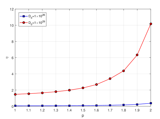
Figure 8: The relation between the power-law index and the required conversion efficiency to fit the Geminga profile.

The preliminary $\gamma$-ray spectrum of HAWC indicates that the electron spectrum cannot be a simple power law, but more likely a power law with a high-energy cutoff (Zhou, 2019). This is also supported by the GeV observation of the Geminga halo (Xi et al., 2019). However, the HAWC $\gamma$-ray spectrum is not broad enough to determine the power-law index $p$. The value of $p=1.0$ is taken from the observation of the X-ray PWN of Geminga (Pavlov et al., 2006). As PWNe can be seen as the sources of the parent electrons of pulsar halos, the X-ray spectrum of PWNe could be used to estimate the low-energy part of the electron injection spectrum. The X-ray PWN of Geminga has a hard photon spectrum with an index of 1.0, corresponding to $p=1.0$ for the electron spectrum.

We give a careful fit to the preliminary $\gamma$-ray spectrum of HAWC (Zhou, 2019) to determine the injection spectrum. The best-fit cutoff energy $E_{c}$ is 133 TeV. The spectral index $p$ is fixed to be 1.0 as suggested by the observations of Geminga’s X-ray PWN. The best-fit $\gamma$-ray spectrum to the HAWC data is shown in Fig. 7.

Furthermore, the power-law indices of PWNe are generally smaller than 2.0 (e.g,, $p=1.8$ for Vela X). The GeV observation of the Geminga halo also indicates $p<2.0$ (Xi et al., 2019). For $p<2.0$, the integral energy of the electron spectrum is concentrated at the high-energy end of the spectrum, which is not seriously affected by the choice of $p$.

In Fig. 8, we show the relation between the power-law index $p$ and the required conversion efficiency $\eta$ to best fit the $\gamma$-ray profile for both the slow-diffusion and fast-diffusion cases. It can be seen that for $p<2.0$, $\eta$ never exceed 100% for the slow-diffusion case, while $\eta$ is always larger than 100% for the fast-diffusion case. Thus, our conclusion is not affected by the assumption of the injection spectrum.

References

- Abeysekara et al. (2017) Abeysekara, A. U., Albert, A., Alfaro, R., et al. 2017, Science, 358, 911, doi: 10.1126/science.aan4880
- Aharonian et al. (2021) Aharonian, F., An, Q., Axikegu, et al. 2021, Phys. Rev. Lett., 126, 241103, doi: 10.1103/PhysRevLett.126.241103
- Aloisio et al. (2009) Aloisio, R., Berezinsky, V., & Gazizov, A. 2009, Astrophys. J., 693, 1275, doi: 10.1088/0004-637x/693/2/1275
- Blumenthal & Gould (1970) Blumenthal, G. R., & Gould, R. J. 1970, Rev. Mod. Phys., 42, 237, doi: 10.1103/RevModPhys.42.237
- Dunkel et al. (2007a) Dunkel, J., Talkner, P., & Hänggi, P. 2007a, Phys. Rev. D, 75, 043001, doi: 10.1103/PhysRevD.75.043001
- Dunkel et al. (2007b) Dunkel, J., Talkner, P., & Hänggi, P. 2007b, New J. Phys., 9, 144, doi: 10.1088/1367-2630/9/5/144
- Fang et al. (2021a) Fang, K., Bi, X.-J., Lin, S.-J., & Yuan, Q. 2021a, Chin. Phys. Lett., 38, 039801, doi: 10.1088/0256-307x/38/3/039801
- Fang et al. (2021b) Fang, K., Xi, S.-Q., & Bi, X.-J. 2021b, Phys. Rev. D, 104, 103024, doi: 10.1103/PhysRevD.104.103024
- Jüttner (1911) Jüttner, F. 1911, Annalen der Physik, 339, 856, doi: https://doi.org/10.1002/andp.19113390503
- Linden et al. (2017) Linden, T., Auchettl, K., Bramante, J., et al. 2017, Phys. Rev. D, 96, 103016, doi: 10.1103/PhysRevD.96.103016
- López-Coto & Giacinti (2018) López-Coto, R., & Giacinti, G. 2018, Mon. Not. Roy. Astron. Soc., 479, 4526, doi: 10.1093/mnras/sty1821
- Pavlov et al. (2006) Pavlov, G. G., Sanwal, D., & Zavlin, V. E. 2006, Astrophys. J., 643, 1146, doi: 10.1086/503250
- Prosekin et al. (2015) Prosekin, A. Y., Kelner, S. R., & Aharonian, F. A. 2015, Phys. Rev. D, 92, 083003, doi: 10.1103/PhysRevD.92.083003
- Recchia et al. (2021) Recchia, S., Di Mauro, M., Aharonian, F. A., et al. 2021, Phys. Rev. D, 104, 123017, doi: 10.1103/PhysRevD.104.123017
- Xi et al. (2019) Xi, S.-Q., Liu, R.-Y., Huang, Z.-Q., Fang, K., & Wang, X.-Y. 2019, Astrophys. J., 878, 104, doi: 10.3847/1538-4357/ab20c9
- Yuan et al. (2017) Yuan, Q., Lin, S.-J., Fang, K., & Bi, X.-J. 2017, Phys. Rev. D, 95, 083007, doi: 10.1103/PhysRevD.95.083007
- Zhou (2019) Zhou, H. 2019, in International Cosmic Ray Conference, Vol. 36, 36th International Cosmic Ray Conference (ICRC2019), 832