Auditing for Diversity using Representative Examples

Abstract

Assessing the diversity of a dataset of information associated with people is crucial before using such data for downstream applications. For a given dataset, this often involves computing the imbalance or disparity in the empirical marginal distribution of a protected attribute (e.g. gender, dialect, etc.). However, real-world datasets, such as images from Google Search or collections of Twitter posts, often do not have protected attributes labeled. Consequently, to derive disparity measures for such datasets, the elements need to hand-labeled or crowd-annotated, which are expensive processes.

We propose a cost-effective approach to approximate the disparity of a given unlabeled dataset, with respect to a protected attribute, using a control set of labeled representative examples. Our proposed algorithm uses the pairwise similarity between elements in the dataset and elements in the control set to effectively bootstrap an approximation to the disparity of the dataset. Importantly, we show that using a control set whose size is much smaller than the size of the dataset is sufficient to achieve a small approximation error. Further, based on our theoretical framework, we also provide an algorithm to construct adaptive control sets that achieve smaller approximation errors than randomly chosen control sets. Simulations on two image datasets and one Twitter dataset demonstrate the efficacy of our approach (using random and adaptive control sets) in auditing the diversity of a wide variety of datasets.

1 Introduction

Mechanisms to audit the diversity of a dataset are necessary to assess the shortcomings of the dataset in representing the underlying distribution accurately. In particular, any dataset containing information about people should suitably represent all social groups (defined by attributes such as gender, race, age, etc.) present in the underlying population in order to mitigate disparate outcomes and impacts in downstream applications [5, 6]. However, many real-world and popular data sources suffer from the problem of disproportionate representation of minority groups [29, 30]. For example, prior work has shown that the top results in Google Image Search for occupations are more gender-biased than the ground truth of the gender distribution in that occupation [20, 35, 8].

Given the existence of biased data collections in mainstream media and web sources, methods to audit the diversity of generic data collections can help quantify and mitigate the existing biases in multiple ways. First, it gives a baseline idea of the demographic distribution in the collection and its deviation from the true distribution of the underlying population. Second, stereotypically-biased representation of a social group in any data collection can lead to further propagation of negative stereotypes associated with the group [17, 36, 10] and/or induce incorrect perceptions about the group [33, 15]. A concrete example is the evidence of stereotype-propagation via biased Google Search results [20, 29]. These stereotypes and biases can be further exacerbated via machine learning models trained on the biased collections [5, 6, 30]. Providing an easy way to audit the diversity in these collections can help the users of such collections assess the potential drawbacks and pitfalls of employing them for downstream applications.

Auditing the diversity of any collection with respect to a protected attribute primarily involves looking at the disparity or imbalance in the empirical marginal distribution of the collection with respect to the protected attribute. For example, from prior work [8], we know that the top 100 Google Image Search results for CEOs in 2019 contained around 89 images of men and 11 images of women; in this case, we can quantify the disparity in this dataset, with respect to gender, as the difference between the fraction of minority group images and the fraction of majority group images, i.e., as $0.11{-}0.89{=}-0.78$. The sign points to the direction of the disparity while the absolute value quantifies the extent of the disparity in the collection. Now suppose that, instead of just 100 images, we had multiple collections with thousands of query-specific images, as in the case of Google Image Search. Since these images have been scraped or generated from different websites, the protected attributes of the people in the images will likely not be labeled at the source. In the absence of protected attribute information, the task of simply auditing the diversity of these large collections (as an end-user) becomes quite labor-intensive. Hand-labeling large collections can be extremely time-expensive, while using crowd-annotation tools (e.g. Mechanical Turk) can be very costly. For a single collection, labeling a small subset (sampled i.i.d. from the collection) can be a reasonable approach to approximate the disparity; however, for multiple collections, this method is still quite expensive since, for every new collection, we will have to re-sample and label a new subset. It also does not support the addition/removal of elements to the collection. One can, alternately, use automated models to infer the protected attributes; although, for most real-world applications, these supervised models need to be trained on large labeled datasets (which may not be available) and pre-trained models might encode their own pre-existing biases [5].

We, therefore, question if there is a cost-effective method to audit the diversity of large collections from a domain when the protected attribute labels of elements in the collections are unknown.

1.1 Our contributions

The primary contribution of this paper is an algorithm to evaluate the diversity of a given unlabeled collection with respect to any protected attribute (Section 3). Our algorithm takes as input the collection to be audited, a small set of labeled representative elements, called the control set, and a metric that quantifies the similarity between any given pair of elements. Using the control set and the similarity metric, our algorithm returns a proxy score of disparity in the collection with respect to the protected attribute. The same control set can be used for auditing the diversity of any collection from the same domain.

The control set and the similarity metric are the two pillars of our algorithm, and we theoretically show the dependence of the effectiveness of our framework on these components. In particular, the proxy measure returned by our algorithm approximates the true disparity measure with high probability, with the approximation error depending on the size and quality of the control set, and the quality of the similarity metric. The protected attributes of the elements of the control set are expected to be labeled; however, the primary advantage of our algorithm is that the size of the control set can be much smaller than the size of the collection to achieve small approximation error (Section 4.2). Empirical evaluations on the Pilots Parliamentary Benchmark (PPB) dataset [5] show that our algorithm, using randomly chosen control sets and cosine similarity metric, can indeed provide a reasonable approximation of the underlying disparity in any given collection (Section 4.1).

To further reduce the approximation error, we propose an algorithm to construct adaptive control sets (Section 5). Given a small labeled auxiliary dataset, our proposed control set construction algorithm selects the elements that can best differentiate between samples with the same protected attribute type and samples with different protected attribute types. We further ensure that the elements in the chosen control set are non-redundant and representative of the underlying population. Simulations on PPB dataset, CelebA dataset [24] and TwitterAAE dataset [3] show that using cosine similarity metric and adaptive control sets, we can effectively approximate the disparity in random and topic-specific collections, with respect to a given protected attribute (Section 6).

1.2 Related work

With rising awareness around the existence and harms of machine and algorithmic biases, prior research has explored and quantified disparities in data collections from various domains. When the dataset in consideration has labeled protected attributes, the task of quantifying the disparity is relatively straightforward. For instance, Davidson et al. [11] demonstrate racial biases in automated offensive language detection by using datasets containing Twitter posts with dialects labeled by the authors or domain experts. Larrazabal et al. [23] can similarly analyze the impact of gender-biased medical imaging datasets since the demographic information associated with the images are available at source. However, as mentioned earlier, protected attribute labels for elements in a collection may not be available, especially if the collection contains elements from different sources.

In the absence of protected attribute labels from the source, crowd-annotation is one way of obtaining these labels and auditing the dataset. To measure the gender-disparity in Google Image Search results, Kay et al. [20] crowd-annotated a small subset of images and compared the gender distribution in this small subset to the true gender distribution in the underlying population. Other papers on diversity evaluation have likewise used a small labeled subset of elements [4, 32] to derive inferences about larger collections. As discussed earlier, the problem with this approach is that it assumes that the disparity in the small labeled subset is a good approximation of the disparity in the given collection. This assumption does not hold when we want to estimate the diversity of a new/multiple collections from the same domain or when elements can be continuously added/removed from the collection. Our method, instead, uses a given small labeled subset to approximate the disparity measure of any collection from the same domain. Semi-supervised learning also explores learning methods that combine labeled and unlabeled samples [38]. The labeled samples are used to train an initial learning model and the unlabeled samples are then employed to improve the model generalizability. Our proposed algorithm has similarities with the semi-supervised self-training approach [2], but is faster and more cost-efficient (Section 4.2).

Representative examples have been used for other bias-mitigation purposes in recent literature. Control or reference sets have been used for gender and skintone-diverse image summarization [8], dialect-diverse Twitter summarization [21], and fair data generation [9]. Kallus et al. [19] also employ reference sets for bias assessments; they approximate the disparate impact of prediction models in the absence of protected attribute labels. In comparison, our goal is to evaluate representational biases in a given collection.

2 Notations

Let $S:=\left\{x_{j}\right\}_{j=1}^{N}$ denote the collection to be evaluated. Each element in the collection consists a $d$-dimensional feature vector $x$, from domain $\mathcal{X}\subseteq\mathbb{R}^{d}$. Every element $j$ in $S$ also has a protected attribute, $z_{j}\in\left\{0,1\right\}$, associated with it; however, we will assume that the protected attributes of the elements in $S$ are unknown. Let $S_{i}:=\left\{x_{j},j\in[N]\mid z_{j}=i\right\}$. A measure of disparity in $S$ with respect to the protected attribute is $d(S):=|S_{0}|/|S|-|S_{1}|/|S|$, i.e., the difference between fraction of elements from group 0 and group 1. A dataset $S$ is considered to be diverse with respect to the protected attribute if this measure is 0, and high $|d(S)|$ implies low diversity in $S$. Our goal will be to estimate this value for any given collection Let $\textrm{p}_{\textrm{data}}$ denote the underlying distribution of the collection $S$.

Control Set.

Let $T$ denote the control set of size $m$, i.e., a small set of representative examples. Every element $T$ also also has a feature vector from domain $\mathcal{X}$ and a protected attribute associated with it. Let $T_{i}:=\left\{x_{j},j\in[m]\mid z_{j}=i\right\}$. Importantly, the protected attributes of the elements in the control set are known and we will primarily employ control sets that have equal number of elements from both protected attribute groups, i.e., $|T_{0}|=|T_{1}|$. The size of control set is also much smaller than the size of the collection being evaluated, i.e., $|T|\ll|S|$. Let $\textrm{p}_{\textrm{control}}$ denote the underlying distribution of the control set $T$.

Throughout the paper, we will also use the notation $a\in b\pm c$ to denote that $a\in[b-c,b+c]$. The problem we tackle in this paper is auditing the diversity of $S$ using $T$; it is formally stated below.

Problem 2.1.

Given a collection $S$ (with unknown protected attributes of elements) and a balanced control set $T$ (with known protected attributes of elements), can we use $T$ to approximate $d(S)$?

3 Model and Algorithm

The main idea behind using the control set $T$ to solve Problem 2.1 is the following: for each element $x\in S$, we can use the partitions $T_{0},T_{1}$ of the control set to check which partition is most similar to $x$. If most elements in $S$ are similar to $T_{0}$, then $S$ can be said to have more elements with protected attribute $z{=}0$ (similarly for $z{=}1$). However, to employ this audit mechanism we need certain conditions on the relevance of the control set $T$, as well as, a metric that can quantify the similarity of an element in $S$ to control set partitions $T_{0},T_{1}$. We tackle each issue independently below.

3.1 Domain-relevance of the control set

To ensure that the chosen control set is representative and relevant to the domain of the collection in question, we will need the following assumption.

Assumption 3.1.

For any $x\in\mathcal{X}$, $\textrm{p}_{\textrm{data}}(x{\mid}z)=\textrm{p}_{\textrm{control}}(x{\mid}z)$, for all $z\in\left\{0,1\right\}$.

This assumption states that the elements of control set are from the have the same conditional distribution as the elements of the collection $S$. It roots out settings where one would try to use non-representative control sets for diversity audits (e.g., full-body images of people to audit the diversity of a collection of portrait images). Note that despite similar conditional distributions, the control set and the collection can (and most often will) have different protected attribute marginal distributions.

We will use the notation $p_{z}(x)$ to denote the conditional distribution of $x$ given $z$ in the rest of the document, i.e., $p_{z}(x):=\textrm{p}_{\textrm{data}}(x\mid z)=\textrm{p}_{\textrm{control}}(x\mid z)$. Given a collection $S$, we will call a control set $T$ (with partitions $T_{0}$, $T_{1}$) domain-relevant if the underlying distribution of $T$ satisfies Assumption 3.1.

3.2 Similarity metrics

Note that even though $p_{z}(x)$ is the same for both the control set and the collection, the distributions $p_{0}(x)$ and $p_{1}(x)$ can be very different from each other, and our aim we will be to design and use similarity metrics that can differentiate between elements from the two conditional distributions.

A general pairwise similarity matrix $\text{sim}:\mathcal{X}\times\mathcal{X}\rightarrow\mathbb{R}_{\geq 0}$ takes as input two elements and returns a non-negative score of similarity between the elements; the higher the score, the more similar are the elements. For our setting we need a similarity metric that can, on average, differentiate between elements that have the same protected attribute type and elements that have different protected attribute types. Formally, we define such a similarity metric as follows.

Definition 3.1 ($\gamma$-similarity metric).

Suppose we are given a similarity metric $\text{sim}:\mathcal{X}\times\mathcal{X}\rightarrow[0,1]$, such that

$$\mathbb{E}_{x_{1},x_{2}\sim p_{z}}\left[\text{sim}(x_{1},x_{2})\right]=\mu_{\textrm{same}}\text{ and }$$

$$\mathbb{E}_{x_{1}\sim p_{z_{1}},x_{2}\sim p_{z_{2}},z_{1}\neq z_{2}}\left[\text{sim}(x_{1},x_{2})\right]=\mu_{\textrm{diff}}.$$

Then for $\gamma\geq 0$, we call sim a $\gamma$-similarity metric if $\mu_{\textrm{same}}-\mu_{\textrm{diff}}\geq\gamma.$

Note that the above definition is not very strict; we do not require $\text{sim}(\cdot,\cdot)$ to return a large similarity score for every pair of elements with same protected attribute type or to return a small similarity score for every pair of elements with different protected attribute types. Rather $\text{sim}(\cdot,\cdot)$, only in expectation, should be able to differentiate between elements from same groups and elements from different groups. In a later section, we show that cosine similarity metric indeed satisfies this condition for real-world datasets.

3.3 Algorithm

Suppose we are given a domain-relevant control set $T$ that satisfies Assumption 3.1 (with partitions $T_{0}$ and $T_{1}$) and a $\gamma$-similarity metric $\text{sim}(\cdot,\cdot)$. With slight abuse of notation, for any element $x\in S$, let $\text{sim}(x,T_{i})=\frac{1}{|T_{i}|}\sum_{y\in T_{i}}\text{sim}(x,y)$ and let $\text{sim}(S,T_{i})=\frac{1}{|S|}\sum_{x\in S}\text{sim}(x,T_{i})$. Let $\hat{d}(S):=\text{sim}(S,T_{0})-\text{sim}(S,T_{1})$. We propose the use of $\hat{d}(S)$ (after appropriate normalization) as a proxy measure for $d(S)$; Algorithm 1 presents the complete details of this proxy diversity score computation and Section 3.4 provides bounds on the approximation error of $\hat{d}(S)$. We will refer to the value returned by Algorithm 1 as DivScore for the rest of the paper.

Algorithm 1 DivScore: Algorithm for proxy diversity audit

Input: Dataset $S$, control set $T:=T_{0}\cup T_{1}$, similarity metric $\text{sim}(\cdot,\cdot)$

1:$l\leftarrow\frac{1}{|T_{0}|\cdot|T_{1}|}\sum_{x,y\in T_{0}\times T_{1}}\text{sim}(x,y)$

2:$u_{0}\leftarrow\frac{1}{|T_{0}|\cdot(|T_{0}|-1)}\sum_{x\in T_{0},y\in T_{0}\setminus\left\{x\right\}}\text{sim}(x,y)$

3:$u_{1}\leftarrow\frac{1}{|T_{1}|\cdot(|T_{1}|-1)}\sum_{x\in T_{1},y\in T_{1}\setminus\left\{x\right\}}\text{sim}(x,y)$

4:Compute $\text{sim}(S,T_{0})\leftarrow\frac{1}{|S|\cdot|T_{0}|}\sum_{x,y\in S\times T_{0}}\text{sim}(x,y)$

5:$s_{0}\leftarrow(\text{sim}(S,T_{0})-l)/(u_{0}-l)$

6:Compute $\text{sim}(S,T_{1})\leftarrow\frac{1}{|S|\cdot|T_{1}|}\sum_{x,y\in S\times T_{1}}\text{sim}(x,y)$

7:$s_{1}\leftarrow(\text{sim}(S,T_{1})-l)/(u_{1}-l)$

8:return $s_{0}-s_{1}$

3.4 Theoretical analysis

To prove that $\hat{d}(S)$ is a good proxy measure for auditing diversity, we first show that if $x\in S_{i}$, then $\text{sim}(x,T_{i})>\text{sim}(x,T_{j})$, for $j=1-i$, with high probability and quantify the exact difference using the following lemma. For the analysis in this section, assume that the elements in $T_{0}$, $T_{1}$ have been sampled i.i.d. from conditional distribution $p_{0},p_{1}$ respectively and $|T_{0}|=|T_{1}|$.

Lemma 3.2.

For $i\in\left\{0,1\right\}$, any $x\in S_{i}$ and $\delta>0$, with probability atleast $1-2e^{-\delta^{2}\mu_{\textrm{diff}}|T|/6}\cdot(1+e^{-\delta^{2}\gamma|T|/6})$, we have

$$\text{sim}(x,T_{i})-\text{sim}(x,T_{1-i})\in\mu_{\textrm{same}}-\mu_{\textrm{diff}}\pm\delta(\mu_{\textrm{same}}+\mu_{\textrm{diff}}).$$ (1)

The lemma basically states that a $\gamma$-similarity metric, with high probability, can differentiate between $\text{sim}(x,T_{i})$ and $\text{sim}(x,T_{1-i})$. The proof uses the fact that since $T$ is domain-relevant and the elements of $T$ are i.i.d. sampled from the conditional distributions, for any $y\in T_{0}$, $\mathbb{E}[\text{sim}(x,y)]=\mu_{\textrm{same}}$ and for any $y\in T_{1}$, $\mathbb{E}[\text{sim}(x,y)]=\mu_{\textrm{diff}}$. Then, the statement of the lemma can be proven using standard Chernoff-Hoeffding concentration inequalities [18, 26]. The complete proof is presented in Appendix A.1. Note that even though sim was defined to differentiate between protected attribute groups in expectation, by averaging over all control set elements in $T_{0},T_{1}$, we are able to differentiate across groups with high probability.

The lemma also partially quantifies the dependence on $|T|$ and $\gamma$. Increasing the size of control set $T$ will lead to higher success probability. Similarly, larger $\gamma$ implies that the similarity metric is more powerful in differentiating between the groups, which also leads to higher success probability. Using the above lemma, we can next prove that the proposed diversity audit measure is indeed a good approximation of the disparity in $S$. Recall that, for the dataset $S$, $\text{sim}(S,T_{i})=\frac{1}{|S|}\sum_{x\in S}\text{sim}(x,T_{i})$.

Theorem 3.3 (Diversity audit measure).

For protected attribute $z\in\left\{0,1\right\}$, let $p_{z}$ denote the underlying conditional distribution $\textrm{p}_{\textrm{data}}(x{\mid}z)$. Suppose we are a given a dataset $S$ containing i.i.d. samples from $\textrm{p}_{\textrm{data}}$, a domain-relevant control set $T$ (with pre-defined partitions by protected attribute $T_{0}$ and $T_{1}$, such that $|T_{0}|=|T_{1}|$) and a similarity metric $\text{sim}:\mathcal{X}^{2}\rightarrow\mathbb{R}_{\geq 0}$, such that if
$\mu_{\textrm{same}}=\mathbb{E}_{x_{0},x_{1}\sim p_{z}}\left[\text{sim}(x_{0},x_{1})\right],$ $\mu_{\textrm{diff}}=\mathbb{E}_{x_{0}\sim p_{0},x_{1}\sim p_{1}}\left[\text{sim}(x_{0},x_{1})\right],$ then $\mu_{\textrm{same}}-\mu_{\textrm{diff}}\geq\gamma$, for $\gamma>0$.

Let $\delta=\sqrt{\frac{6\log(20|S|)}{|T|\min(\mu_{\textrm{diff}},\gamma)}}$ and let $\hat{d}(S):=\text{sim}(S,T_{0})-\text{sim}(S,T_{1})$. Then, with high probability, $\hat{d}(S)/(\mu_{\textrm{same}}-\mu_{\textrm{diff}})$ approximates $d(S)$ within an additive error of $\delta\cdot(\mu_{\textrm{same}}+\mu_{\textrm{diff}})/(\mu_{\textrm{same}}-\mu_{\textrm{diff}})$.

In particular, with probability $\gtrapprox$ 0.9,

$$\hat{d}(S)\in(\mu_{\textrm{same}}-\mu_{\textrm{diff}})\cdot d(S)\pm\delta\cdot(\mu_{\textrm{same}}+\mu_{\textrm{diff}}).$$

Theorem 3.3 states that, with high probability, $d(S)$ is contained in a small range of values determined by $\hat{d}(S)$, i.e.,

$$d(S)\in\left(\hat{d}(S)\pm\delta\cdot(\mu_{\textrm{same}}+\mu_{\textrm{diff}})\right)/\left(\mu_{\textrm{same}}-\mu_{\textrm{diff}})\right).$$

The theoretical analysis is line with the implementation in Algorithm 1 (DivScore), i.e., the algorithm computes $\hat{d}(S)$ and normalizes it appropriately using estimates of $\mu_{\textrm{same}}$ and $\mu_{\textrm{diff}}$ derived from the control set. The proof is presented in Appendix A.2.

Note that Theorem 3.3 assumes that $\mu_{\textrm{same}}{=}\mathbb{E}_{x_{0},x_{1}\sim p_{z}}\left[\text{sim}(x_{0},x_{1})\right]$ is the same for both $z\in\left\{0,1\right\}$. However, they may not be same in practice and DivScore uses separate upper bounds for $z{=}0$ and $z{=}1$ ($u_{0}$ and $u_{1}$ respectively). Similarly, we don’t necessarily require a balanced control set (although, as discussed in Section 4.2, a balanced control set is preferable over an imbalanced one). We keep the theoretical analysis simple for clarity, but both these changes can be incorporated in Theorem 3.3 to derive similar bounds as well.

The dependence of error on $\gamma$ and $T$ can also be inferred from Theorem 3.3. The denominator in the error term in Theorem 3.3 is lower bounded by $\gamma$. Therefore, the larger the $\gamma$, the lower is the error and the tighter is the bound. The theorem also gives us an idea of the size of control set required to achieve low $\delta$ error and high success probability. To keep $\delta$ small, we can choose a control set $T$ with $|T|=\Omega\left(\log|S|\right)$. In other words, a control set of size $c\log|S|$ elements, for an appropriate $c>1$, should be sufficient to obtain low approximation error. Since the control sets are expected to have protected attribute labels (to construct partitions $T_{0}$ and $T_{1}$), having small control sets will make the usage of our audit algorithm much more tractable.

Cost of DivScore.

The time complexity of Algorithm 1 (DivScore) is $O(|S|{\cdot}|T|)$, and it only requires $|T|$ samples (control set) to be labeled. In comparison, if one was to label the entire collection to derive $d(S)$, the time complexity would be $O(|S|)$, but all $|S|$ samples would need to be labeled. With a control set $T$ of size $\Omega\left(\log|S|\right)$, our approach is much more cost-effective. The elements of $T$ are also not dependent on elements of $S$; hence, the same control set can be used for other collections from the same domain.

(a) Gender protected attribute

(b) Skin-tone protected attribute

Figure 1: Results for PPB-2017 dataset using random and adaptive control sets. The reported performance is the mean of output from DivScore across 100 repetitions (errorbars denote standard error). To improve readability, we limit the y-axis to range to $[-1.5,1.5]$, which results in trimmed errorbands for some methods; we present the same expanded plots without axis restrictions in Appendix C. The protected attribute considered here are gender and skintone. The x-axis reports the fraction of $z=0$ images in the collection ($\in\left\{0,0.1,0.2,\dots,1.0\right\}$) and, for each collection, we report the following five metrics in y-axis: true disparity of the collection, DivScore-Random-Balanced, DivScore-Random-Proportional, IID-Measure, and DivScore-Adaptive. A collection is considered diverse if the diversity score (y-axis) is 0; the larger the deviation of diversity score from 0, the lower the diversity is in the evaluated collection. Amongst all metrics, DivScore-Adaptive, IID-Measure, and SS-ST seem to have the lowest standard error. However, using IID-Measure and SS-ST are much costlier than DivScore, as discussed in Section 4.2.

4 Empirical Evaluation Using Random Control Sets

We first demonstrate the efficacy of the DivScore algorithm on a real-world dataset using random, domain-relevant control sets.

4.1 PPB-2017 dataset

The PPB (Pilots Parliamentary Benchmark) dataset consists of 1270 portrait images of parliamentarians from six different countries. The images in this dataset are labeled with gender (male vs female) and skin-tone (values are the 6 types from the Fitzpatrick skin-type scale [14]) of the person in the image. This dataset was constructed and curated by Buolamwini and Gebru [5]. We will use gender and skintone as the protected attributes for our diversity audit analysis.

Methodology.

We first the split the dataset into two parts: the first containing 200 images and the second containing 1070 images. The first partition is used to construct control sets, while the second partition is used for diversity audit evaluation. Since we have the gender and skin-tone labels for all images, we can construct sub-datasets of size 500 with custom distribution of protected attribute types. In other words, for a given $f\in\left\{0,0.1,0.2,\dots,1.0\right\}$, we construct a sub-dataset $S$ of the second partition containing $f\cdot|S|$ images corresponding to protected attribute $z=0$. Hence, by applying Algorithm 1 (DivScore) using a given control set $T$, we can assess the performance of our proxy measure for collection with varying fraction of under/over-represented group elements.

When protected attribute is gender, $z=0$ will denote $g=\text{female}$, when protected attribute is skin-tone, $z=0$ will denote $s>3$ (skin-tone types corresponding to dark-skin), and when protected attribute is intersection of gender and skin-tone, $z=0$ will denote $g=\text{female and }s>3$ (corresponding to dark-skinned women).

Control sets.

To evaluate the performance of DivScore the selection of elements for the control sets (of size 50 from the first partition) can be done in multiple ways: (1) random balanced control sets, i.e., randomly block-sampled control sets with equal number of $z{=}0$ and $z{=}1$ images; (2) random proportional control sets, i.e., control sets i.i.d. sampled from the collection in question; (3) adaptive control sets, i.e., non-redundant control sets that can best differentiate between samples with the same protected attribute type and samples with different protected attribute types. The complete details of construction of adaptive control sets is given in Section 5; in this section, we primarily focus on performance of DivScore when using random control sets. We will refer to our method as DivScore-Random-Balanced, when using random balanced control sets, and as DivScore-Random-Proportional, when using random proportional control sets. In expectation, random proportional control sets will have a similar empirical marginal distribution of protected attribute types as the collection; correspondingly, we also report the disparity measure of the random proportional control set $d(T)$ as a baseline. We will refer to this baseline as IID-Measure. Random proportional control sets need to be separately constructed for each new collection, while the same random balanced control set can be used for all collections; we discuss this contrast further in Section 4.2.

We also implement a semi-supervised self-training algorithm as a baseline. This algorithm (described formally in Appendix B) iteratively labels the protected attribute of those elements in the dataset for which similarity to one group in the control set is significantly larger than similarity to the other group. It then uses the learnt labels to compute the diversity score. We implement this baseline using random control sets and refer to it as SS-ST.

Similarity Metric.

We construct feature vector representations for all images in the dataset using pre-trained deep image networks. The feature extraction details are presented in Appendix B. Given the feature vectors, we use the cosine similarity metric to compute pairwise similarity between images. In particular, given feature vectors $x_{1},x_{2}$ corresponding to any two images, we will define the similarity between the elements as

$$\text{sim}(x_{1},x_{2})=1+\frac{x_{1}^{\top}x_{2}}{\lVert x_{1}\rVert\lVert x_{2}\rVert}.$$

We add 1 to the standard cosine between two vectors to ensure that the similarity values are always non-negative.

Evaluation Measures.

We repeat the simulation 100 times; for each repetition, we construct a new split of the dataset and sample a new control set. We report the true fraction $f$ and the mean (and standard error) of all metrics across all repetitions.

Results.

The results are presented in Figure 1 (the figure also plots the performance of DivScore-Adaptive, that is discussed in Section 5). With respect to gender, Figure 1a shows that the DivScore measure is always close to the true disparity measure for all collections, and the standard error of all metrics is quite low. In this case, random control sets (balanced or proportional) can indeed approximate the disparity of all collections with very small error.

The results are more mixed when skintone is the protected attribute. Figure 1b shows that while the DivScore average is close to the true disparity measure, the standard errors are quite high. The baselines IID-Measure and SS-ST have lower errors than our proxy measure (although they are not a feasible method for real-world applications, as discussed in the next section). The poor performance for this protected attribute, when using random control sets, suggests that strategies to construct good non-random control sets are necessary to reduce the approximation error.

4.2 Discussion

Drawbacks of IID-Measure.

Recall that IID-Measure essentially uniformly samples a small subset of elements of the collection and reports the disparity of this small subset. Figure 1 shows that this baseline indeed performs well for PPB-dataset. However, it is not a cost-effective approach for real-world disparity audit applications. The main drawback of this baseline is that the subset has to have i.i.d. elements from the collection being audited for it to accurately predict the disparity of the collection. This implies that, for every new collection, we will have to re-sample and label a small subset to audit its diversity using IID-Measure. It is unreasonable to apply this approach when there are multiple collections (from the same domain) that need to be audited or when elements are continuously being added/removed from the collection. The same reasoning limits the applicability of DivScore-Random-Proportional.

DivScore-Random-Balanced, on the other hand, addresses this drawback by using a generic labeled control set that can be used for any collection from the same domain, without additional overhead of constructing a new control set everytime. This is also why balanced control sets should be preferred over imbalanced control sets, since a balanced control set will be more adept at handling collections with varying protected attribute marginal distributions.

Drawbacks of SS-ST.

The semi-supervised learning baseline SS-ST has larger estimation bias than DivScore-Random-Balanced and DivScore-Random-Proportional, but has lower approximation error than these methods. However, the main drawback of this baseline is the time complexity. Since it iteratively labels elements and then adds them to control set to use for future iterations, the time complexity of this baseline is quadratic in dataset size. In comparison, the time complexity of DivScore is linear in the dataset size.

Dependence on $\gamma$.

The performance of DivScore on PPB-dataset highlights the dependence of approximation error on the $\gamma$. Since the gender and skintone labels of images in the dataset are available, we can empirically derive the $\gamma$ value for each protected attribute using the cosine similarity metric. When gender is the protected attribute, $\gamma$ is around 0.35. On the other hand, when skintone is the protected attribute, $\gamma$ is 0.08. In other words, the cosine similarity metric is able to differentiate between images of men and women to a better extent than between images of dark-skinned and light-skinned people. This difference in $\gamma$ is the reason for the relatively larger error of DivScore in case of skintone protected attribute.

Cosine similarity metric.

The simulations also show that measuring similarity between images using the cosine similarity metric over feature vectors from pre-trained networks is indeed a reasonable strategy for disparity measurement. Pre-trained image networks and cosine similarity metric has similarly also been used in prior work for classification and clustering purposes [28, 37]. Intuitively, cosine similarity metric is effective when conditional distributions $p_{0}$ and $p_{1}$ are concentrated over separate clusters over the feature space; e.g., for PPB-dataset and gender protected attribute, the high value of $\gamma$ (0.35) provides evidence of this phenomenon. In this case, cosine similarity can, on average, differentiate between elements from same cluster and different clusters.

Dependence on $|T|$.

The size of control set is another factor which is inversely related to the error of the proxy disparity measure. For this section, we use control sets of size 50. Smaller control sets lead to larger variance, as seen in Figure 5 in the Appendix, while using larger control sets might be inhibitory and expensive since, in a real-world applications, protected attributes of the control set images need to be hand-labeled or crowd-annotated.

Nevertheless, these empirical results highlight the crucial dependence on $\gamma$ and properties of the control set $T$. In the next section, we improve upon the performance of our disparity measure and reduce the approximation error by designing non-random control sets that can better differentiate across the protected attribute types.

Algorithm 2 Algorithm to construct an adaptive control set

Input: Auxiliary set $U=U_{0}{\cup}U_{1}$, similarity metric sim, $m$, $\alpha\geq 0$

1:$T_{0},T_{1},\gamma_{0},\gamma_{1}\leftarrow\emptyset$

2:for $i\in\left\{0,1\right\}$ do

3:     for $x\in U_{i}$ do

4:          $\gamma_{i}^{(x)}{\leftarrow}\frac{1}{|U_{i}|-1}\sum\limits_{y\in U_{i}\setminus\left\{x\right\}}\text{sim}(x,y){-}\frac{1}{|U_{1-i}|}\sum\limits_{y\in U_{1-i}}\text{sim}(x,y)$

5:     end for

6:     while $|T_{i}|<m/2$ do

7:          $T_{i}\leftarrow T_{i}\cup\left\{\arg\max\left\{\gamma_{i}^{(x)}-\alpha\cdot\max_{y\in T_{i}}\text{sim}(x,y)\right\}_{x\in U_{i}\setminus T_{i}}\right\}$

8:     end while

9:end for

10:return $T_{0}\cup T_{1}$

5 Adaptive Control Sets

The theoretical analysis in Section 3.4 and the simulations in Section 4.1 use random control sets; i.e., $T$ contains i.i.d. samples from $p_{0}$ and $p_{1}$ conditional distributions. This choice was partly necessary because the error depends on the $\gamma$-value of the similarity metric, which is quantified as $\mu_{\textrm{same}}-\mu_{\textrm{diff}}$, where

$$\mu_{\textrm{same}}{=}\mathbb{E}_{x_{0},x_{1}\sim p_{z}}\left[\text{sim}(x_{0},x_{1})\right],\;\;\;\mu_{\textrm{diff}}{=}\mathbb{E}_{x_{0}\sim p_{0},x_{1}\sim p_{1}}\left[\text{sim}(x_{0},x_{1})\right].$$

However, quantifying $\mu_{\textrm{same}},\mu_{\textrm{diff}}$ (and, hence, $\gamma$) using expectation over the entire distribution might be unnecessary.

In particular, the theoretical analysis uses $\mu_{\textrm{same}}$ to quantify $\mathbb{E}_{x\sim p_{i}}\left[\text{sim}(x,T_{i})\right]$, for any $i\in\left\{0,1\right\}$ (similarly $\mu_{\textrm{diff}}$). Hence, we require the difference between $\mu_{\textrm{same}}$ and $\mu_{\textrm{diff}}$ to be large only when comparing the elements from the underlying distribution to the elements in the control set. This simple insight provides us a way to choose good control sets; i.e., we can choose control sets $T$ for which the difference $|\mathbb{E}_{x}\left[\text{sim}(x,T_{i})\right]-\mathbb{E}_{x}\left[\text{sim}(x,T_{1-i})\right]|$ is large.

Control sets that maximize $\gamma$.

Suppose we are given an auxiliary set $U$ of i.i.d. samples from $\textrm{p}_{\textrm{data}}$, such that the protected attributes of elements in $U$ are known. Let $U_{0},U_{1}$ denote the partitions with respect to the protected attribute. Once again, $U\ll|S|$ and $U$ will be used to construct a control set $T$. Let $m{\in}\left\{0,2,4,\dots,|U|\right\}$ denote the desired size of $T$. For each $i{\in}\left\{0,1\right\}$ and $y{\in}U_{i}$, we can first compute

$$\gamma_{i}^{(y)}:=\mathbb{E}_{x\sim U_{i}\setminus\left\{y\right\}}\left[\text{sim}(x,y)\right]-\mathbb{E}_{x\sim U_{1-i}\setminus\left\{y\right\}}\left[\text{sim}(x,y)\right],$$

and then construct a control set $T$ by adding $m/2$ elements from each $U_{i}$ with the largest values in the set $\left\{\gamma_{i}^{(y)}\right\}_{y\in U_{i}}$ to $T$.

Figure 2: Results for CelebA dataset. For each feature, we plot the true gender disparity score for that feature as well as the scores obtained using DivScore-Random-Balanced and DivScore-Adaptive approaches. For both methods, the control set size is kept to 50. Note that the error of DivScore-Adaptive is much smaller in this case.

Reducing redundancy in control sets.

While the above methodology will result in control sets that maximize the difference between similarity with same group elements vs similarity with different group elements, it can also lead to redundancy in the control set. For instance, if two elements in $U$ are very similar to each other, they will large pairwise similarity and can, therefore, both have large $\gamma_{i}^{(y)}$ value ; however, adding both to the control set is redundant. Instead, we should aim to make the control set as diverse and representative of the underlying population as possible. To that end, we employ a Maximal Marginal Relevance (MMR)-type approach and iteratively add elements from $U$ to the control set $T$. For the first $m/2$ iterations, we add elements from $U_{0}$ to $T$. Given a hyper-parameter $\alpha\geq 0$, at any iteration $t$, the element added to $T$ is the one that maximizes the following score:

$$\left\{\gamma_{0}^{(y)}-\alpha\cdot\max_{x\in T}\text{sim}(x,y)\right\}_{y\in U_{0}\setminus T}.$$

The next $m/2$ iterations similarly adds elements from $U_{1}$ to $T$ using $\gamma_{1}^{(y)}$. The quantity $\max_{x\in T}\text{sim}(x,y)$ is the redundancy score of $y$; i.e., the maximum similarity of $y$ with any element already added to $T$. By penalizing an element for being very similar to an existing an element in $T$, we can ensure that chosen set $T$ is diverse. The complete algorithm to construct such a control set, using a given $U$, is provided in Algorithm 2. We will refer to the control sets constructed using Algorithm 2 as adaptive control sets and Algorithm 1 with adaptive control sets as DivScore-Adaptive.

Note that, even with this control set construction method, the theoretical analysis does not change. Given any control set $T$ ($=T_{0}\cup T_{1}$), let $\gamma^{(T)}:=\mathbb{E}_{i}\left[\mathbb{E}_{x\in p_{i}}\left[\text{sim}(x,T_{i})\right]-\mathbb{E}_{x\sim p_{1-i}}\left[\text{sim}(x,T_{1-i})\right]\right].$ For a control set $T$ with parameter $\gamma^{(T)}$, we can obtain the high probability bound in Theorem 3.3 by simply replacing $\gamma$ by $\gamma^{(T)}$. Infact, since we are explicitly choosing elements that have large $\gamma_{i}^{(\cdot)}$ parameters, $\gamma^{(T)}$ is expected to be larger than $\gamma$ and, hence, using the an adaptive control set will lead to a stronger bound in Theorem 3.3.

Our algorithm uses the standard MMR framework to reduce redundancy in the control set. Importantly, prior work has shown that the greedy approach of selecting the best available element is indeed approximately optimal [7]. Other non-redundancy approaches, e.g., Determinantal Point Processes [22], can also be employed.

Cost of each method.

DivScore-Adaptive requires an auxiliary labeled set $U$ from which we extract a good control set. Since $|U|>|T|$, the cost (in terms of time and labeling required) of using DivScore-Adaptive is slightly larger than the cost of using DivScore-Random-Balanced, for which we just need to randomly sample $|T|$ elements to get a control set. However, results in Appendix C show that, to achieve similar approximation error, the required size of adaptive control sets is smaller than the size of random control sets. Hence, even though adaptive control sets are more costly to construct, DivScore-Adaptive is more cost-effective for disparity evaluations and requires smaller control sets (compared to DivScore-Random-Balanced) to approximate with low error.

6 Empirical Evaluation using adaptive control sets

6.1 PPB-2017

Once again, we first test the performance of adaptive control sets on PPB-2017 dataset. Recall that we split the dataset into two parts of size 200 and 1070 each. Here, the first partition serves as the auxiliary set $U$ for Algorithm 2. The input hyper-parameter $\alpha$ is set to be 1. The rest of the setup is the same as in Section 4.1.

Results.

The results for this simulation are presented in Figure 1 (in red). The plots show that, using adaptive control sets, we obtain sharper proxy diversity measures for both gender and skintone. For skintone protected attribute, the standard error of DivScore-Adaptive is significantly lower than DivScore-Random-Balanced.

Note that the average of DivScore-Adaptive, across repetitions, does not align with the true disparity measure (unlike the results in case of random control sets). This is because the adaptive control sets do not necessarily represent a uniformly random sample from the underlying conditional distributions. Rather, they are the subset of images from $U$ with best scope of differentiating between images from different protected attributes types. This non-random construction of the control sets leads to a possibly-biased but tighter approximation for the true disparity in the collection.

As noted before, when using adaptive control sets (from Algorithm 2), the performance depends on the measure $\gamma^{(T)}:=\mathbb{E}_{i}\left[\mathbb{E}_{x\in p_{i}}\left[\text{sim}(x,T_{i})\right]-\mathbb{E}_{x\sim p_{1-i}}\left[\text{sim}(x,T_{1-i})\right]\right].$ By construction, we want to choose control sets $T$ for which $\gamma^{(T)}$ is greater than the $\gamma$ value over the entire distribution. Indeed, in case of PPB dataset and for every protected attribute, we observe that $\gamma^{(T)}$ values of the adaptive control sets are much larger than the corresponding value when of randomly chosen control sets. When gender is the protected attribute, on average, $\gamma^{(T)}$ is 0.96 (for random control sets, it was 0.35). Similarly, when skintone is the protected attribute, $\gamma^{(T)}$ is around 0.34 (for random control sets, it was 0.08). The stark improvement in these values, compared to random control sets, is the reason behind the increased effectiveness of adaptive control sets in approximating the disparity of the collection.

6.2 CelebA dataset

CelebA dataset [24] contains images of celebrities with tagged facial attributes, such as whether the person in the image has eyeglasses, mustache, etc., along with the gender of the person in the image. We use 29 of these attributes and a random subset of around 20k images for our evaluation. The goal is to approximate the disparity in the collection of images corresponding to a given facial attribute.

Methodology.

We evaluate the performance DivScore-Random-Balanced and DivScore-Adaptive for this dataset. We perform 25 repetitions; in each repetition, an auxiliary set $U$ is sampled of size 500 (and removed from the main dataset) and used to construct either a random control set (of size 50) or an adaptive control set (of size 50). The chosen control set is kept to be the same for all attribute-specific collections in a repetition. For each image, we use the pre-trained image networks to extract feature vectors (see Appendix B for details) and the cosine similarity metric - Eqn $\eqref{2}$ - to compute pairwise similarity.

Results.

The results are presented in Figure 2. The plot shows that, for almost all attributes, the score returned by DivScore-Adaptive is close to the true disparity score and has smaller error than DivScore-Random-Balanced. Unlike the collections analyzed in PPB evaluation, the attribute-specific collections of CelebA dataset are non-random; i.e., they are not i.i.d. samples from the underlying distribution. Nevertheless, DivScore-Adaptive is able to approximate the true disparity for each attribute-specific collection quite accurately.

Note that, for these attribute-specific collections, implementing IID-Measure would be very expensive, since one would have to sample a small set of elements for each attribute and label them. In comparison, our approach uses the same control set for all attributes and, hence, is much more cost-effective.

Figure 3: Results for TwittterAAE dataset with dialect as the protected attribute for DivScore-Random-Balanced and DivScore-Adaptive using control sets of size 50.

6.3 TwitterAAE dataset

To show the effectiveness of DivScore beyond image datasets, we analyze the performance on a dataset of Twitter posts. The TwitterAAE dataset, constructed by Blodgett et al. [3], contains around 60 million Twitter posts. We filter the dataset to contain only posts which either are certainly written in the African-American English (AAE) dialect (100k posts) or the White English dialect (WHE) (1.06 million posts). The details of filtering and feature extraction using a pre-trained Word2Vec model [25] are given in Appendix B.

Methodology.

For this dataset, we will evaluate the performance of DivScore-Random-Balanced and DivScore-Adaptive. We partition the datasets into two parts: the first contains 200 posts and the second contains the rest. The first partition is used to construct control sets of size 50 (randomly chosen from first partition for DivScore-Random-Balanced and using Algorithm 2 for DivScore-Adaptive). The protected attribute is the dialect of the post. The second partition is used for diversity audit evaluation. We construct sub-datasets or collections with custom distribution of posts from each dialect. For a given $f\in\left\{0,0.1,\dots,1.0\right\}$, we construct a sub-dataset $S$ of the second partition containing $f\cdot|S|$ AAE posts. The overall size of the sampled collection is kept to be 1000 and we perform 25 repetitions. For DivScore-Adaptive, we use $\alpha=0.1$.

Results.

The audit results for collections from TwitterAAE dataset are presented in Figure 3. The plot shows that both DivScore-Random-Balanced and DivScore-Adaptive can, on expectation, approximate the disparity for all collections; the disparity estimate from both methods increases with increasing fraction of AAE posts in the collection. However, once again, the approximation error of DivScore-Adaptive is smaller than the approximation error of DivScore-Random-Balanced in most cases.

7 Applications, Limitations & Future Work

In this section, we discuss the potential applications of our framework, some practical limitations and directions for future work.

Third-party implementations and auditing summaries.

To audit the diversity of any collection, DivScore simply requires access to a small labeled control set and a similarity metric. The cost of constructing these components is relatively small (compared to labeling the entire collection) and, hence, our audit framework can be potentially employed by third-party agencies that audit independently of the organization owning/providing the collections. For instance, our algorithm can be implemented as a browser plugin to audit the gender diversity of Google Image results or the dialect diversity of Twitter search results. Such a domain-generic diversity audit mechanism can be used to ensure a more-balanced power dynamic between the organizations disseminating/controlling the data and the users of the applications that use this data.

Variable-sized collections.

DivScore can easily adapt to updates to the collections being audited. If an element is added/removed, one simply needs to add/remove the contribution of this element from $\text{sim}(S,T_{0})$ and $\text{sim}(S,T_{1})$, and recompute $\hat{d}(S)$. This feature crucially addresses the main drawback of IID-Measure.

Possibility of stereotype exaggeration.

In our simulations, we evaluate the gender diversity using “male” vs “female” partition and skintone diversity using the Fitzpatrick scale. Pre-defined protected attribute partitions, however, can be problematic; e.g., commercial AI tools’ inability in handling non-binary gender [31].

Considering that Our algorithm is based on choosing control sets that can differentiate across protected attribute types, there is a possibility that the automatically constructed control sets can be stereotypically-biased. For example, a control set with high $\gamma^{(T)}$ value for gender may just include images of men and women, and exclude images of transgender individuals. While non-redundancy aims to ensure that the control set is diverse, it does not guarantee that the control set will be perfectly representative. Given this possibility, we strongly encourage the additional hand-curation of automatically-constructed control sets. Further, any agency using control sets should make them public and elicit community feedback to avoid representational biases. Recent work on designs for such cooperative frameworks can be employed for this purpose [27, 13].

Choice of $\alpha$.

For DivScore-Adaptive, $\alpha$ is the parameter that controls the redundancy of the control set. It primarily depends on the domain in consideration and we use fixed $\alpha$ for collections from the same domain. However, the mechanism to choose the best $\alpha$ for a given domain is unclear and can be further explored.

Improving theoretical bounds.

While the theoretical bounds provide intuition about dependence of error on size of control set and $\gamma$, the constants in the bounds can be further improved. E.g., in case of PPB dataset with gender protected attribute and the empirical setup in Section 4.1, Theorem 3.3 suggests that error $|\delta|\leq 5$; however, we observe that the error is much smaller ($\leq 0.5$) in practice. Improved and tighter analysis can help reduce the difference between theoretical and empirical performance.

Assessing qualitative disparities.

Our approach is more cost-effective than crowd annotation. However, crowd-annotation can help answer questions about the collection beyond disparity quantification. For example, Kay et al. [20] use crowd-annotation to provide evidence of sexualized depictions of women in Google Image results for certain occupations such as construction worker. As part of future work, one can explore extensions of our approach or control sets that can assess such qualitative disparities as well.

8 Conclusion

We propose a method, DivScore, to audit the diversity of any given collection using a small control set and an algorithm to construct adaptive control sets. Theoretical analysis shows that DivScore approximates the disparity of the collection, given appropriate control sets and similarity metrics. Empirical evaluations demonstrate that DivScore can handle collections from both image and text domains.

Appendix A Proofs

A.1 Proof of Lemma 3.2

Proof of Lemma 3.2.

Suppose $x$ has protected attribute type 0, i.e., $x\in S_{0}$. Since control set $T$ is domain-relevant, we know that for any $y\in T_{0}$, $\mathbb{E}[\text{sim}(x,y)]=\mu_{\textrm{same}}$ and for any $y\in T_{1}$, $\mathbb{E}[\text{sim}(x,y)]=\mu_{\textrm{diff}}$. Then, using Chernoff-Hoeffding bounds [18, 26], we get that for any $\delta>0$,

$$\mathbb{P}\left[\text{sim}(x,T_{0})\notin(1\pm\delta)\mu_{\textrm{same}}\right]\leq 2\exp(-\delta^{2}\cdot|T_{0}|\cdot\mu_{\textrm{same}}/3),\textrm{ and }$$

$$\mathbb{P}\left[\text{sim}(x,T_{1})\notin(1\pm\delta)\mu_{\textrm{diff}}\right]\leq 2\exp(-\delta^{2}\cdot|T_{1}|\cdot\mu_{\textrm{diff}}/3).$$

Note that $|T_{0}|=|T_{1}|=|T|/2$. The probability that both the above events are simultaneously satisfied is

$$2\exp(-\delta^{2} \mu_{\textrm{same}}|T|/6)+2\exp(-\delta^{2}\mu_{\textrm{diff}}|T|/6)$$

$$\leq 2\exp(-\delta^{2}\mu_{\textrm{diff}}|T|/6)\cdot\left(1+\exp(-\delta^{2}\gamma|T|/6)\right).$$

Therefore, combining the two statements we get that with probability atleast $1-2\exp(-\delta^{2}\mu_{\textrm{diff}}|T|/6)\cdot\left(1+\exp(-\delta^{2}\gamma|T|/6)\right)$,

$$\text{sim}(x,T_{0})-\text{sim}(x,T_{1})$$

$$\in\left[(1-\delta)\mu_{\textrm{same}}-(1+\delta)\mu_{\textrm{diff}},(1+\delta)\mu_{\textrm{same}}-(1-\delta)\mu_{\textrm{diff}}\right]).$$

Simplifying the above expression, we get

$$\text{sim}(x,T_{i})-\text{sim}(x,T_{1-i})\in\mu_{\textrm{same}}-\mu_{\textrm{diff}}\pm\delta(\mu_{\textrm{same}}+\mu_{\textrm{diff}}).$$

The other direction (when $x\in S_{1}$) follows from symmetry. ∎

A.2 Proof of Theorem 3.3

Proof of Theorem 3.3.

Applying Lemma 3.2 to each element in $S$, we get that with probability atleast $q:=1-2|S|e^{-\delta^{2}\mu_{\textrm{diff}}|T|/6}\cdot(1+e^{-\delta^{2}\gamma|T|/6})$, all elements satisfy condition (1). Summing up $\text{sim}(x,T_{0})-\text{sim}(x,T_{1})$ for all $x\in S$, we get

$$\text{sim}(S,T_{0})- \text{sim}(S,T_{1})$$

$$\in(\mu_{\textrm{same}}-\mu_{\textrm{diff}})\cdot\left(|S_{0}|-|S_{1}|\right)/|S|\pm\delta(\mu_{\textrm{same}}+\mu_{\textrm{diff}}).$$

Simplifying the above bound, we have that with probability $q$,

$$\hat{d}(S)\in(\mu_{\textrm{same}}-\mu_{\textrm{diff}})\cdot d(S)\pm\delta\cdot(\mu_{\textrm{same}}+\mu_{\textrm{diff}}).$$

By choosing $\delta=\sqrt{\frac{6\log(20|S|)}{|T|\min(\mu_{\textrm{diff}},\lambda)}}$, the probability $q$ is atleast

$$1- 2|S|e^{-\delta^{2}\mu_{\textrm{diff}}|T|/6}(1+e^{-\delta^{2}\gamma|T|/6})$$

$$\geq 1-2|S|e^{-\log 20|S|}(1+e^{-\log 20|S|})=0.9-\frac{1}{200|S|}.$$

∎

Appendix B Implementation Details

Details of SS-ST baseline.

The complete implementation of the semi-supervised self-training baseline SS-ST is given in Algorithm 3. We use $k=5$ for PPB-2017 simulations.

Algorithm 3 SS-ST baseline

Input: Dataset $S$, control set $T:=T_{0}\cup T_{1}$, $\text{sim}(\cdot,\cdot)$, $k\in\mathbb{Z}_{>0}$

1:$n_{0},n_{1}\leftarrow 0$

2:while $S\neq\emptyset$ do

3:     for $x\in S$ do

4:         $s(x)\leftarrow\frac{1}{|T_{0}|}\sum_{y\in T_{0}}\text{sim}(x,y)-\frac{1}{|T_{1}|}\sum_{y\in T_{1}}\text{sim}(x,y)$

5:     end for

6:     $\tilde{T}\leftarrow$ top $k$ elements in set $\left\{|s(x)|\right\}_{x\in S}$

7:     $n_{0}\leftarrow n_{0}+|\left\{s(x)\mid x\in\tilde{T},s(x)>0\right\}|$

8:     $n_{1}\leftarrow n_{1}+|\left\{s(x)\mid x\in\tilde{T},s(x)<0\right\}|$

9:     $S\leftarrow S\setminus\tilde{T},T\leftarrow T\cup\tilde{T}$

10:end while

11:return $(n_{0}-n_{1})/|S|$

PPB-2017 and CelebA datasets.

For both PPB-2017 and CelebA datasets, feature extraction for images is done using the pre-trained VGG-16 deep network [34]. The network has been pre-trained on the Imagenet [12] dataset. To extract the feature of any given image, we pass it as input to the network and extract the 4096-dimensional weight vector of the last fully connected layer. We further reduce the feature vector size to 300 by performing PCA on the set of features of all images in the dataset.

TwitterAAE dataset.

For the TwitterAAE dataset, the authors constructed a demographic language identification model to report the probability of each post being written by a user of any of the following population categories: non-Hispanic Whites, non-Hispanic Blacks, Hispanics, and Asians. We filter the dataset to contain only posts for which probability of belonging to non-Hispanic African-American English language model or non-Hispanic White English language model is $\geq 0.99$. This leads to a dataset of around 1.2 million tweets, with around 100k posts belonging to non-Hispanic African-American English language model and 1.06 million posts belonging to non-Hispanic White English language model; we will refer to the two groups of posts as AAE and WHE posts in.

To extract feature vectors corresponding to the Twitter posts, we use a Word2Vec model [25] pre-trained on 400 million Twitter posts [16]. For any given post, we first use the Word2Vec model to extract features for every word in the post. Then we take the average of the word features to obtain the feature of the post.

(a) Gender protected attribute

(b) Skin-tone protected attribute

Figure 4: Results for PPB-2017 dataset using random and adaptive control sets. The plots in this figure are the same as the plots in Figure 1, except that we don’t put y-axis limitations here to present the complete errorbars for all methods.

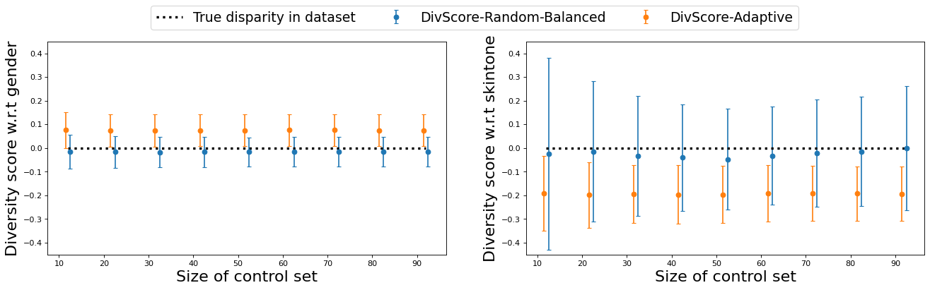
(a) Gender protected attribute

(b) Skin-tone protected attribute

Figure 5: Results for PPB-2017 dataset using different sized random and adaptive control sets.

Figure 6: Performance of DivScore-Random-Proportional and IID-Measure on CelebA dataset

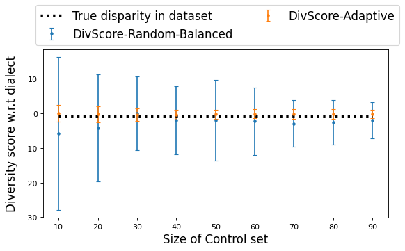
Figure 7: Results for TwitterAAE dataset using different sized random and adaptive control sets.

Appendix C Other Empirical Results

Alternate Figure 1 plot.

First, we present the plots from Figure 1 without y-axis limitations. This is presented in Figure 4.

Variation of performance with control set size for PPB-dataset.

Figure 5 presents the variation of disparity measure with control set size. The disparity in the collection is fixed to be 0. The plots show that DivScore-Adaptive can achieve low approximation error using smaller sized control sets than DivScore-Random-Balanced.

Performance of DivScore-Random-Proportional and IID-Measure on CelebA dataset.

Figure 6 presents the performance of DivScore-Random-Proportional and IID-Measure on for different facial attributes of CelebA dataset. As expected, IID-Measure has low approximation error, while DivScore-Random-Proportional has low approximation error for some attributes and high error for others. Nevertheless, as discussed in Section 4.2, both baselines need different control sets for collections corresponding to different attributes, and hence, are costly when auditing multiple collections from the same domain.

Variation of performance with control set size for TwitterAAE-dataset.

Figure 7 presents the variation of disparity measure with control set size. The disparity in the collection is fixed to be -0.826 (which is the disparity of the overall dataset) The plots show that, once again, DivScore-Adaptive can achieve low approximation error using much smaller sized control sets than DivScore-Random-Balanced.

References

- [1]
- Bair [2013] Eric Bair. 2013. Semi-supervised clustering methods. Wiley Interdisciplinary Reviews: Computational Statistics 5, 5 (2013), 349–361.
- Blodgett et al. [2016] Su Lin Blodgett, Lisa Green, and Brendan O’Connor. 2016. Demographic Dialectal Variation in Social Media: A Case Study of African-American English. In Proceedings of Conference on Empirical Methods in Natural Language Processing.
- Bolukbasi et al. [2016] Tolga Bolukbasi, Kai-Wei Chang, James Y Zou, Venkatesh Saligrama, and Adam T Kalai. 2016. Man is to computer programmer as woman is to homemaker? debiasing word embeddings. In Advances in Neural Information Processing Systems.
- Buolamwini and Gebru [2018] Joy Buolamwini and Timnit Gebru. 2018. Gender shades: Intersectional accuracy disparities in commercial gender classification. In FAT* 2018. 77–91.
- Caliskan et al. [2017] Aylin Caliskan, Joanna J Bryson, and Arvind Narayanan. 2017. Semantics derived automatically from language corpora contain human-like biases. Science (2017).
- Carbonell and Goldstein [1998] Jaime G Carbonell and Jade Goldstein. 1998. The use of MMR, diversity-based reranking for reordering documents and producing summaries.. In SIGIR, Vol. 98.
- Celis and Keswani [2020] L Elisa Celis and Vijay Keswani. 2020. Implicit Diversity in Image Summarization. Proceedings of the ACM on Human-Computer Interaction 4, CSCW2 (2020), 1–28.
- Choi et al. [2020] Kristy Choi, Aditya Grover, Trisha Singh, Rui Shu, and Stefano Ermon. 2020. Fair generative modeling via weak supervision. In ICML. PMLR.
- Collins [2002] Patricia Hill Collins. 2002. Black feminist thought: Knowledge, consciousness, and the politics of empowerment. routledge.
- Davidson et al. [2019] Thomas Davidson, Debasmita Bhattacharya, and Ingmar Weber. 2019. Racial Bias in Hate Speech and Abusive Language Detection Datasets. In Proceedings of the Third Workshop on Abusive Language Online. 25–35.
- Deng et al. [2009] Jia Deng, Wei Dong, Richard Socher, Li-Jia Li, Kai Li, and Li Fei-Fei. 2009. Imagenet: A large-scale hierarchical image database. In 2009 IEEE conference on computer vision and pattern recognition. Ieee, 248–255.
- Finnegan et al. [2015] Eimear Finnegan, Jane Oakhill, and Alan Garnham. 2015. Counter-stereotypical pictures as a strategy for overcoming spontaneous gender stereotypes. Frontiers in psychology 6 (2015), 1291.
- Fitzpatrick [2008] T Fitzpatrick. 2008. Fitzpatrick Skin Type Classification Scale. Skin Inc (2008).
- Gerbner et al. [1986] George Gerbner, Larry Gross, Michael Morgan, and Nancy Signorielli. 1986. Living with television: The dynamics of the cultivation process. Perspectives on media effects 1986 (1986), 17–40.
- Godin [2019] Fréderic Godin. 2019. Improving and Interpreting Neural Networks for Word-Level Prediction Tasks in Natural Language Processing. Ghent University (2019).
- Harris [1982] Trudier Harris. 1982. From mammies to militants: Domestics in black American literature. Temple University Press.
- Hoeffding [1994] Wassily Hoeffding. 1994. Probability inequalities for sums of bounded random variables. In The Collected Works of Wassily Hoeffding. Springer, 409–426.
- Kallus et al. [2020] Nathan Kallus, Xiaojie Mao, and Angela Zhou. 2020. Assessing algorithmic fairness with unobserved protected class using data combination. In Proceedings of the 2020 Conference on Fairness, Accountability, and Transparency. 110–110.
- Kay et al. [2015] Matthew Kay, Cynthia Matuszek, and Sean A Munson. 2015. Unequal representation and gender stereotypes in image search results for occupations. In Proceedings of ACM Conference on Human Factors in Computing Systems.
- Keswani and Celis [2021] Vijay Keswani and L Elisa Celis. 2021. Dialect Diversity in Text Summarization on Twitter. The Web Conference’2021 (2021).
- Kulesza et al. [2012] Alex Kulesza, Ben Taskar, et al. 2012. Determinantal point processes for machine learning. Foundations and Trends® in Machine Learning 5, 2–3 (2012), 123–286.
- Larrazabal et al. [2020] Agostina J Larrazabal, Nicolás Nieto, Victoria Peterson, Diego H Milone, and Enzo Ferrante. 2020. Gender imbalance in medical imaging datasets produces biased classifiers for computer-aided diagnosis. Proceedings of the National Academy of Sciences 117, 23 (2020), 12592–12594.
- Liu et al. [2015] Ziwei Liu, Ping Luo, Xiaogang Wang, and Xiaoou Tang. 2015. Deep Learning Face Attributes in the Wild. In ICCV 2015.
- Mikolov et al. [2015] Tomas Mikolov, Kai Chen, Gregory S Corrado, and Jeffrey A Dean. 2015. Computing numeric representations of words in a high-dimensional space. US Patent 9,037,464.
- Mitzenmacher and Upfal [2017] Michael Mitzenmacher and Eli Upfal. 2017. Probability and computing: Randomization and probabilistic techniques in algorithms and data analysis.
- Muller et al. [2020] Michael Muller, Cecilia Aragon, Shion Guha, Marina Kogan, Gina Neff, Cathrine Seidelin, Katie Shilton, and Anissa Tanweer. 2020. Interrogating Data Science. In Conference Companion Publication of the 2020 on CSCW. 467–473.
- Nguyen and Bai [2010] Hieu V Nguyen and Li Bai. 2010. Cosine similarity metric learning for face verification. In Asian conference on computer vision. Springer, 709–720.
- Noble [2018] Safiya Umoja Noble. 2018. Algorithms of oppression: How search engines reinforce racism. nyu Press.
- O’neil [2016] Cathy O’neil. 2016. Weapons of math destruction: How big data increases inequality and threatens democracy. Broadway Books.
- Scheuerman et al. [2019] Morgan Klaus Scheuerman, Jacob M Paul, and Jed R Brubaker. 2019. How Computers See Gender: An Evaluation of Gender Classification in Commercial Facial Analysis Services. Proceedings of ACM Human-Computer Interaction (2019).
- Schwemmer et al. [2020] Carsten Schwemmer, Carly Knight, Emily D Bello-Pardo, Stan Oklobdzija, Martijn Schoonvelde, and Jeffrey W Lockhart. 2020. Diagnosing gender bias in image recognition systems. Socius 6 (2020), 2378023120967171.
- Shrum [1995] Larry J Shrum. 1995. Assessing the social influence of television: A social cognition perspective on cultivation effects. Communication Research 22, 4 (1995).
- Simonyan and Zisserman [2014] Karen Simonyan and Andrew Zisserman. 2014. Very deep convolutional networks for large-scale image recognition. arXiv preprint arXiv:1409.1556 (2014).
- Singh et al. [2020] Vivek K Singh, Mary Chayko, Raj Inamdar, and Diana Floegel. 2020. Female Librarians and Male Computer Programmers? Gender Bias in Occupational Images on Digital Media Platforms. Journal of the Association for Information Science and Technology (2020).
- Word et al. [1974] Carl O Word, Mark P Zanna, and Joel Cooper. 1974. The nonverbal mediation of self-fulfilling prophecies in interracial interaction. Journal of experimental social psychology 10, 2 (1974), 109–120.
- Xing et al. [2003] Eric P Xing, Michael I Jordan, Stuart J Russell, and Andrew Y Ng. 2003. Distance metric learning with application to clustering with side-information. In NIPS.
- Zhu and Goldberg [2009] Xiaojin Zhu and Andrew B Goldberg. 2009. Introduction to semi-supervised learning. Synthesis lectures on artificial intelligence and machine learning (2009).